
Challenges in Quantifying Losses in a Partly Urbanised Catchment: A South Australian Case Study


UniSA STEM, Mawson Lakes Campus, University of South Australia, Mawson Lakes, SA 5095, Australia
*
Author to whom correspondence should be addressed.
Water 2022, 14(8), 1313; https://doi.org/10.3390/w14081313
Submission received: 8 March 2022
/
Revised: 13 April 2022
/
Accepted: 15 April 2022
/
Published: 18 April 2022
(This article belongs to the Section Urban Water Management)
Abstract
:Quantifying hydrological losses in a catchment is crucial for developing an effective flood forecasting system and estimating design floods. This can be a complicated and challenging task when the catchment is urbanised as the interaction of pervious and impervious (both directly connected and indirectly connected) areas makes responses to rainfall hard to predict. This paper presents the challenges faced in estimating initial losses (IL) and proportional losses (PL) of the partly urbanised Brownhill Creek catchment in South Australia. The loss components were calculated for 57 runoff generating rainfall events using the non-parametric IL-PL method and parametric method based on two runoff routing models, Runoff Routing Burroughs (RORB) and Rainfall-Runoff Routing (RRR). The analysis showed that the RORB model provided the most representative median IL and PL for the rural portion of the study area as 9 mm and 0.81, respectively. However, none of the methods can provide a reliable loss value for the urban portion because there is no runoff contribution from unconnected areas for each event. However, the estimated non-parametric IL of 1.37 mm can be considered as IL of EIA of the urban portion. Several challenges were identified in the loss estimation process, mainly when selecting appropriate storm events, collecting data with the available temporal resolution, extracting baseflow, and determining the main-stream transmission losses, which reduced the urban flow by 5.7%. The effect of hydrograph shape in non-parametric loss estimation and how combined runoff from the effective impervious area and unconnected (combined indirectly connected impervious and pervious) areas affects the loss estimation process using the RORB and RRR models are further discussed. We also demonstrate the importance of identifying the catchment specific conditions appropriately when quantifying baseflow and runoff of selected events for loss estimation.
1. Introduction
One of the most critical issues associated with the prediction of urban floods is determining catchment response to rainfall, which impacts the delay in flow through the catchment and the hydrological losses that determine what proportion of catchment rainfall appears as runoff. Hydrological loss is defined as precipitation that does not appear as direct runoff and is attributed to interception by vegetation, infiltration into the soil, evaporation, retention on the surface (depression storage), and transmission loss through the stream bed and banks as per Australian Rainfall & Runoff, 2016 [1].
Estimating hydrological loss for a catchment is complicated by several factors including catchment topography, soil characteristics, and climate [2,3]. While several recent studies have identified methods to quantify losses in rural Australian catchments in for the purpose of design flood estimation and forecasting [4,5,6,7], literature on loss estimation for urban and partly urbanised catchments is limited [8]. Urban catchments contain a significant proportion of impervious areas (directly connected impervious areas (DCIA) and indirectly connected impervious areas (ICIA)) that challenge urban loss estimation, as the response of the impervious areas is notably different to that of the pervious areas. Further, accurate determination of urban loss depends on an estimation of unconnected areas (a combination of ICIA and pervious areas), and effective impervious area (EIA) of the catchment, which are generally difficult to quantify [9]. Phillips et al. [8] suggested that EIA was roughly 70–80% of DCIA when the DCIA was obtained based on the GIS based mapping analysis of a catchment. Other conceptual methods, including regression analysis, calibration of a rainfall-runoff model, and direct analysis of rainfall and streamflow records have been highlighted in Book 5 of ARR 2019 as suitable techniques to estimate EIA [10].
Several loss models have been used to estimate hydrological losses in Australia and elsewhere. These models are categorised into three main types; simple, empirical, and process models under Chapter 3, Book 5 of ARR, 2016 [10]. The simple models estimate the infiltration portion of the total runoff as losses, and evaporation and depression losses are ignored. The Green–Ampt, Horton, Philip, and Richards equations are simple and widely used models in many studies [11,12,13]. The process models consider a complex steps to consider flow through the surface and soil layers [14]. Empirical models typically provide lump-sum loss value at the catchment scale and conceptualise the loss elements from interception, depressions and infiltration [15,16]. Therefore, many studies have utilised empirical models rather than simple and process models to estimate losses. The most rainfall runoff excess models, including the Initial Loss-Continuing Loss model (IL-CL), the Initial Loss-Proportional Loss model (IL-PL), SCS Curve Number method, Variable Continuing Losses model, and Soil Water balance Model (SWMOD), fall within this empirical category [17,18,19]. Out of these models, the IL-CL and IL-PL have been widely used to estimate losses in Australian catchments [4,16,20,21]. Initial loss (IL) occurs before the start of surface runoff, while continuing loss (CL) and proportional loss (PL) occur throughout the remainder of the storm. Although Lang et al. [6] and Hill et al. [5] have indicated that the IL-CL loss model was the best loss model for design flood estimation, Dyer et al. [22] and Goyen [23] have shown that the IL-PL model outperforms the IL-CL model. Further, the PL rate varies during the rainfall period, which is one of the advantages over the CL [5]. Additionally, some rainfall-runoff models such as RORB have recommended using IL-PL over IL-CL model for urban and partly urbanised catchments [24]. However, research on using the IL-PL loss model for urban loss estimation is limited [5,25].
Losses can be estimated using either parametric or non-parametric method. The simple non-parametric method widely used in many Australian studies uses the catchment’s water balance to estimate losses [6,26]. However, Hill et al. [5] argued that loss values based on this approach were highly subjective, relating largely to the hydrograph shape. Alternatively, loss values can be determined using runoff routing models based on the observed rainfall and runoff data and model specific parameters [27]. In these parametric methods, loss values are adjusted until the rainfall excess hydrograph shows the best fit with the recorded hydrograph [24]. As noted earlier, runoff in an urban catchment is a combined output of EIA and unconnected areas, which are difficult to quantify, but rainfall-runoff routing models should have the capacity to model the combined runoff of these two areas. By comparison, many models do not assess the EIA and unconnected area losses separately [8]. Table 1 compares the rainfall-runoff models that can be used to estimate IL-PL loss from the recorded storm events. Though the listed rainfall and runoff models are similar, RORB is the commonly used runoff routing program to quantify losses from the Australian catchments. The ‘ROR’ of ‘RORB’ stands for ‘runoff routing’. The ‘B’ no longer has significance but at one time indicated that the program was developed and maintained on a Burroughs B6700 computer [24]. The main reasons for this extensive use of the RORB model are free access and minimum required inputs. The other advantage of using the RORB model is that the results can be easily compared with the already available literature. However, there are some significant challenges to be overcome when using RORB to estimate the runoff [28]. One of the limitations is that the result of the model depends on the number of sub-areas [22]. Further, RORB estimates the losses using one runoff process based on the unconnected area. Therefore, a more reliable loss estimation can be obtained if a model with two or three runoff processes can be used.
RORB is a commonly used runoff routing model in Australia [6,21,32] and recommends IL-PL loss models for urban catchments [24]. One drawback of RORB is that it is a single runoff process that assesses losses using only the surface runoff process. The latest version of RORB (version 6.45) can consider losses from DCIA, ICIA, and pervious area separately for urban and partly urbanised catchments. However, RORB does not calculate loss contributions separately. Instead, it factors the losses across the components. Therefore, it is still challenging to identify loss from EIA and unconnected areas for urban catchments using the RORB model.
Kemp [28] introduced an alternate runoff routing model, namely the Rainfall-Runoff Routing (RRR) model, which can also be used to estimate losses from rural and urban catchments. The RRR uses the IL-PL loss model, and it is capable of modelling three processes, namely slow flow (subsurface), fast flow (surface), and baseflow processes. The other advantage of the RRR model is that it can estimate losses from the impervious and pervious areas of an urban catchment separately. Despite these attractions, the version of this updated RRR model is not yet available in the public domain. In addition, the spatial variability of rainfall cannot be accounted for in RRR, as it is still a single node model [28].
Channel transmission loss (TL) is the streamflow reduction due to water absorbed through the stream bed and banks, evaporation, and infiltration from floodplains when runoff travels away from the stream [10,33,34]. Like other losses, TL varies both spatially and temporally, and changes the input hydrograph for the runoff routing model. Therefore, for a reliable account of losses, accurate estimation of the TL of the stream is a critical factor in the water balance of a catchment. Several approaches, including regression models, differential equations, and field experiments, have been used to estimate TLs of the natural channels [35,36,37,38]. However, most of these models are complex and require more data than is generally available. Further, developed methods using these approaches are always unique to the case-study catchment and are therefore challenging to transfer to other catchments. McMahon et al. [39] found that most research used a simple water balance equation to estimate TL, and recommended additionally considering groundwater inflow, evaporation losses and bed infiltration with inflow and outflow to calculate TL. However, a lack of required field data resolution [40] and data uncertainty [41] make adding these functions challenging.
Depending on focus and research objectives, studies followed different criteria to select rainfall events for modelling. Criteria used to define rainfall events include depth, duration, inter-event gap and temporal pattern [21,42]. Selection based only on these few criteria may not be sufficient for loss estimation of the urban catchments for flash flood purposes. Thus, priority should also be given to modelling runoff generated by high intensity storm events. Flash flood is rapid flooding usually occurs within less than six hours of the intense rainfall events [43,44]. When estimating losses for urban flash flooding using historical storm events, short-duration rainfall bursts that generate runoff from EIA and unconnected areas should be used. However, high-intensity, short-duration events that produce runoff from unconnected urban areas are uncommon, and only a few historical events are available in SA for urban catchments [45]. Therefore, obtaining sufficient high intensity events for such catchments to estimate losses is a challenge.
The work presented here is part of the first author’s PhD research project, which investigates relationships between initial soil moisture content and the initial loss. The case study catchment selected in this research is Brownhill Creek (BHC), a partly urbanised catchment in the SA metropolitan region. The work involved in this analysis included data collection and preparation, storm event selection, and rainfall-runoff modelling for calculating losses. During this investigation, we came across several challenges when:
- Selecting storm events for the determination of partly urban losses.
- Selecting the most appropriate temporal resolution of the storm event.
- Extracting baseflow using Lyne and Hollick algorithm.
- Estimating transmission loss
- Choosing loss estimation method between the parametric and non-parametric for the rural and urban portions of the study area.
This paper aims to explain the strategies we adopted to overcome the above challenges.
2. Materials and Methods
2.1. Study Area
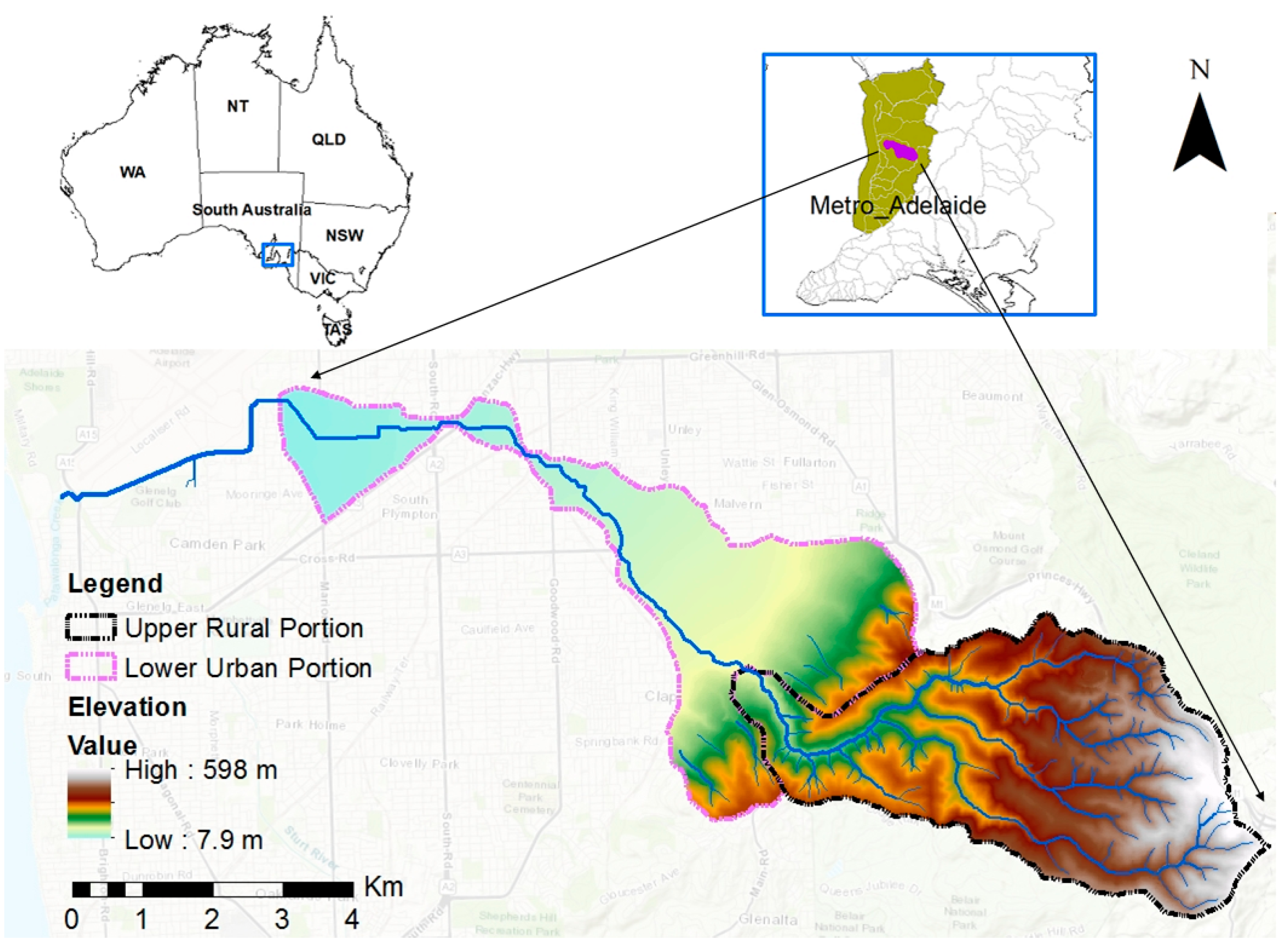
The Brownhill Creek (BHC) catchment is a small, partly urbanised catchment located in the eastern Adelaide metropolitan region of South Australia (Figure 1). It extends for approximately 24 km from the Mount Lofty Ranges to Patawalonga Lake before discharging into Holdfast Bay. The study area has a Mediterranean climate with a comparatively dry summer and wet winter.
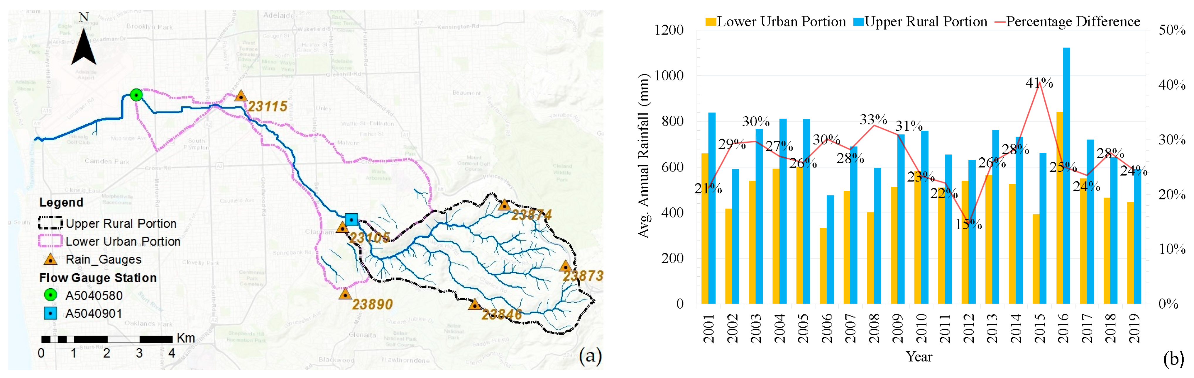
The study area consists of two sub-catchments defined by gauging stations, as shown in Figure 2a. The upper catchment (rural portion) has an area of approximately 17.9 km2, zoned as a hill face, with limited development potential. The lower catchment (urban portion) covers 14 km2 with areas of low relief and substantial urban land use. A piped urban drainage system collects surface runoff from this portion of the catchment before discharging into Brownhill Creek at several locations. A considerable part of the creek (more than 18% of the channel length) in this urban portion has been modified into concrete-lined and masonry channels during the urban development process [46].
Observed data from six rainfall gauging stations and two flow gauge stations in the study area were used for this analysis (Figure 2a). Annual average rainfall variation from 2001 to 2019 (Figure 2b) shows that the upper rural portion of the catchment, receives between 15% to 41% more rainfall than the lower urban portion. Based on historical flood data, BHC has been categorised as a high-risk floodplain for flash floods in SA [47].
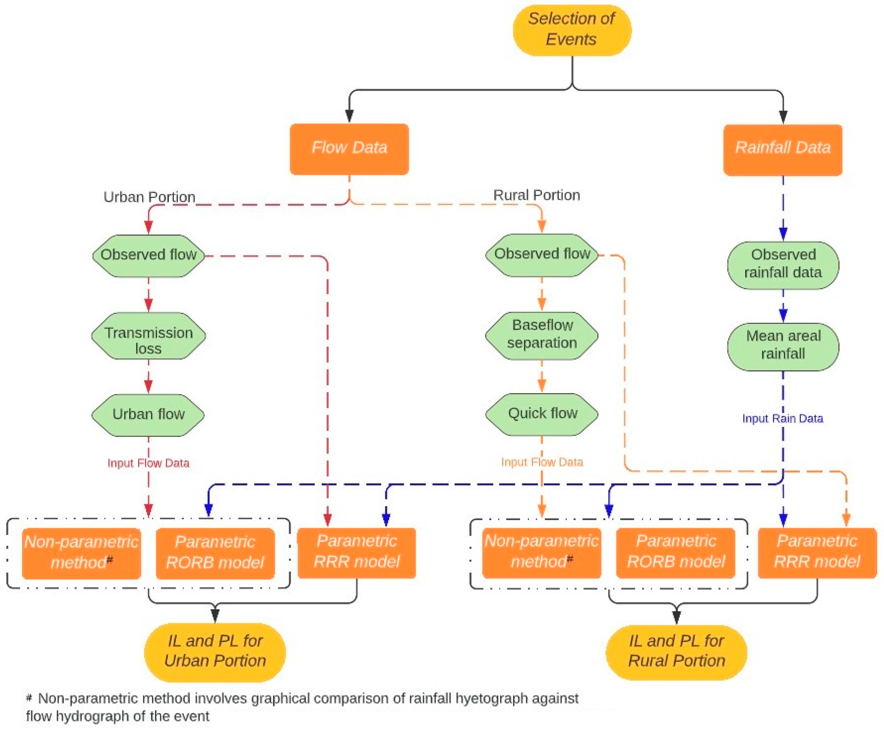
2.2. Methodology
The nature of the BHC catchment is partly urbanised. The literature supports the loss estimation using IL-PL over IL-CL for such catchments [22,23]. The recommended approach to loss estimation using the RORB rainfall-runoff model that we adopt for this investigation is also IL-PL [24]. Hence, IL-PL was considered to be the most appropriate empirical approach to quantify losses in the BHC catchment. A systematic approach presented in Figure 3 was used to conduct this assessment and details of individual steps are detailed in following sections.
2.2.1. Selection of the Events
Runoff generating events with lower annual exceedance probability (AEP, less frequent events) were prioritised as the focus of the study is to quantify losses for urban flash flooding. However, some additional criteria need to be identified to select the appropriate storm events.
Selecting a method to choose the storm events for loss estimation is a challenge because no recommended criteria are available. The literature showed that different criteria were used in various studies depending on the purpose of the loss estimation. For example, Rahman et al. [48] defined a rainfall event using three rainfall characteristics, namely rainfall duration, intensity, and temporal pattern, when estimating the hydrological losses for design flood estimation of rural catchments in Victoria, Australia. Slightly different criteria, such as cumulative depth of rainfall (10 mm), no rainfall between the storm events (5 h), maximum intensity (0.25 m/h), and maximum rainfall during (1.2 mm) within a 6 h dry period, were used by Gamage et al. [20] to select the complete storm events for the loss calculation of SA rural catchments. Hill et al. [5] defined the complete storm using 12 h. inter-event gap and the end time when surface runoff had effectively ended for the loss assessment of 38 rural catchments in Australia. When it comes to the urban loss estimation, event selection criteria are again different from the rural catchment. For example, Phillips et al. [8] adopted some criteria when they extracted storm events to estimate losses for the urban catchment in Australia. The current study is also to assess the losses from the urban catchment in Australia. Therefore, it was decided to use the criteria listed in Table 2 adopted by Phillips et al. [8]. The end of runoff for each event was determined by taking the earliest overlap between recorded and baseflow hydrographs. When runoff overlapped with a following event, the end point of the runoff for the first event was taken as the starting time of the following event.
2.2.2. Rainfall Data Preparation
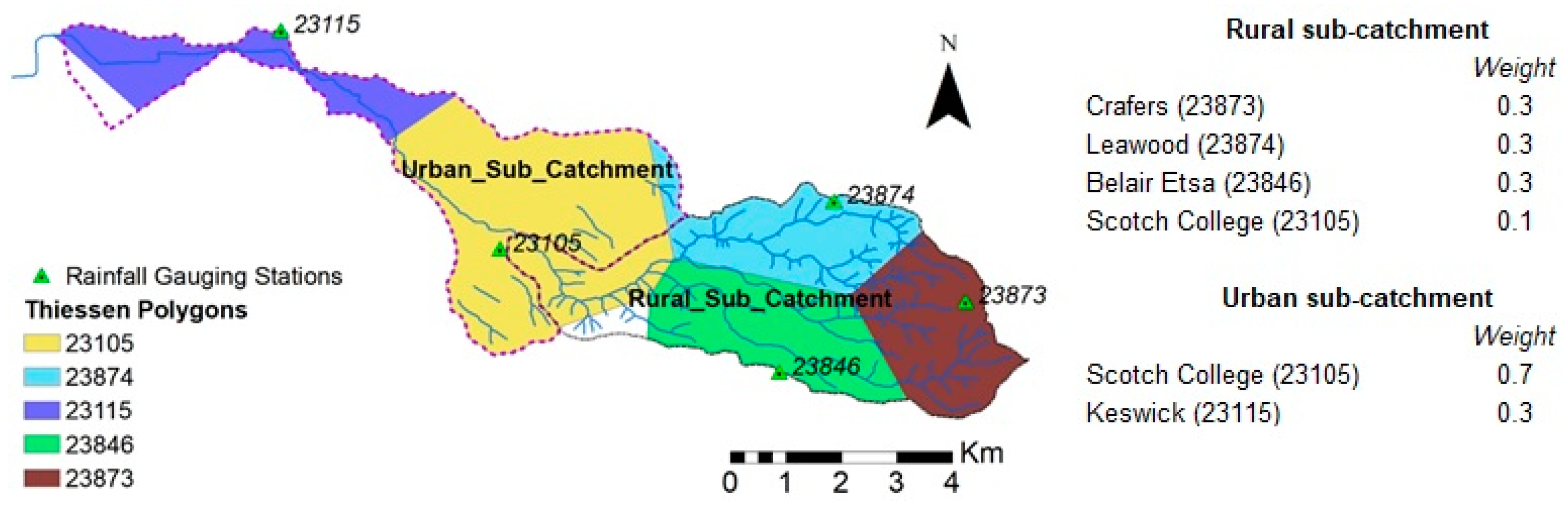
The catchment weighted average rainfall of the selected events was obtained using the Thiessen Polygon feature under the Analysis toolbox in ArcGIS 10.7. Figure 4 shows the Thiessen Polygon areas and the relative weights used for each gauging station when obtaining the mean catchment rainfall. Based on the extracted events, we observed that time to peak was between 5 and 12 h for the rural portion while that was only between 3 and 6.5 h for the urban portion. Therefore, we considered that the catchment response time is quick for the study catchment. Hence, rainfall and runoff data at 15 min steps were used.
2.2.3. Flow Preparation–Upper Rural Portion
The baseflow must be separated using an external algorithm from the observed streamflow hydrographs before using it to the non-parametric method and RORB model for the upper catchment. However, the RRR model uses the observed flow as it can separate quick flow and baseflow.
Baseflow separation can be done by graphical methods or more automated digital filter techniques [49]. Many review studies showed that the digital filter techniques had been used over the graphical separation methods in recent studies [50,51]. Lyne and Holick, Chapman, Furey and Gupta, and Eckhardt algorithms are some of the most commonly used approaches. Latuamury et al. [52] showed that Eckhardt’s filters, a two-parameter digital filter performed better than the other algorithms for small island watersheds in Indonesia. Chapman et al. [53] criticised the Lyne–Hollick filter method for assuming a constant baseflow during no quick flow. However, a few studies showed no significant difference in the outcome using Lyne and Holick and Chapman techniques [51]. In addition, Zhang et al. [54] recommended the Lyne–Holick method by using five catchments in Eastern Australia. The same method was suggested by Kang et al. [55] using some catchment data in the Nakdong River in the Republic of Korea. Further, the Lyne–Holick filter method has been widely used with daily and hourly data for catchments across Australia [49]. Because of these reasons, and given this study is based on the Australian catchment data and follows ARR recommendations, the Lyne and Hollick filter, Equation (1), was used to separate baseflow from the observed flow [56]. One of the advantages of using the Lyne–Holick filter method is that the results can be easily compared with the other Australian based studies. However, Eckhardt [57] showed that the catchment size and conditions influenced filtering results. So, a comparison of baseflow using a few other filter methods would provide a chance to select a better method for the study area.
where is the filtered quick response at the sampling instant. is the observed streamflow, and ‘a’ is the filter parameter (recession constant).
fk = afk−1 + 1/2(Yk − Yk−1)(1 + a)
The Lyne and Hollick algorithm commonly uses three passes with a filter parameter value of 0.925 for daily data sets [58]. Evans et al. [59] have suggested some modifications to the Lyne and Hollick algorithm when using smaller time step data. Rachel et al. [60] found that nine passes with a filter parameter value of 0.925 is suitable for a 1-h time step which was then used by several studies to extract baseflow [26,49,54,61]. This study also used a filter parameter of 0.925 for our 15 min time step as we could find no studies supporting shorter time steps.
2.2.4. Flow Preparation–Lower Urban Portion
A significant part of the urban portion’s runoff resulted from EIA, while the remainder was inflow from the upper portion and so did not contribute to baseflow. Therefore, baseflow separation was not necessary for the downstream urban part of the catchment. The travel time between the two gauging stations was found to be approximately 1 h [62], and when a 1-h lagged inflow hydrograph from the upstream station was compared to the hydrograph at the downstream station, TL was evident within the urban channel. TL was excluded from the inflow hydrograph by considering the simple water balance of inflow and outflow. For consistency, TL was estimated for the selected events in the following manner. First, this TL assessment was performed for each 15 min time interval. Then, event TL was obtained by adding all 15 min TL together for the entire event duration:
- If there is no inflow from the upper portion, it is taken that there is no TL.
- If the lagged inflow is greater than the outflow, then the flow difference is taken as the TL.
- At certain time steps of the event, the lagged inflow can be less than the outflow. In such cases, TL cannot be derived directly, and an estimated value was used for each 15 min time interval which was the average TL value obtained for 15 min on the rest of the event duration.
2.2.5. Estimation of IL and PL by Non-Parametric Method
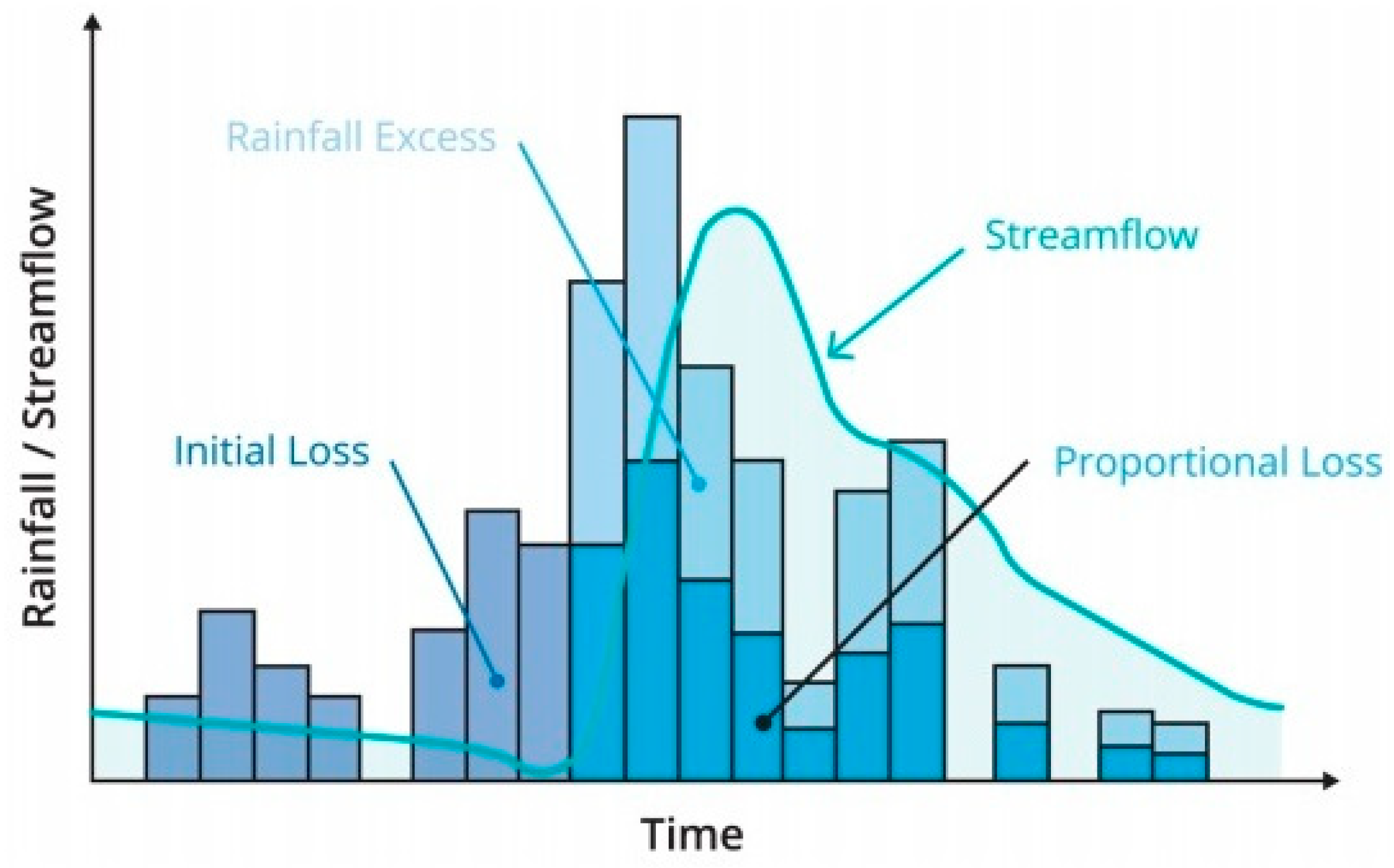
Figure 5 shows a rainfall hyetograph and corresponding hydrograph for a typical storm event along with an IL-PL loss model. In calculating IL and PL with this approach, quick flow (total flow−baseflow) was used for the upper rural portion, while urban streamflow (total flow−inflow−transmission losses) was used for the lower urban portion.
The flow depth in mm was calculated by using Equation (2), where is the filtered flow in m3/s for the time interval, Δt is the time step in seconds, and A is the catchment area in m2.
The PL is the proportion of the rainfall lost at each time step after the IL has been satisfied. The PL was obtained using Equation (3) [20].
TSV is the total surface runoff volume in m3 from Equation (4), and TRV is the total rainfall volume in m3 from and Equation (5).
where is the 15 min rainfall in mm during the time interval and n is the total number of time steps within the storm duration.
2.2.6. Estimation of IL-PL by Parametric Method-RORB
The storm file and catchment file for each event were prepared as per steps recommended in the RORB manual. The 15-min mean catchment rainfall (Section 2.2.2) and instantaneous flow (Section 2.2.3 and Section 2.2.4) were used when developing storm files for the selected events.
When the catchment and storm files were prepared for an event, the RORB model calibration was performed through an interactive trial and error fitting procedure by changing model parameters (m, kc and IL). The model automatically adjusts the PL value at each calibration run to give the best fit between the observed and the modelled hydrographs. The model parameters that provided the best overall fit were considered essential when fitting the hydrographs, and the errors in peak discharge were used as the objective function and kept minimal.
Losses calculated using the RORB model for the rural portion represented the accumulated losses from the pervious areas of each sub-area. Hence, the impervious fraction computed using Google Maps for each sub-area was used as an input to the catchment file. However, a different approach was taken for the urban portion, as EIA and unconnected area contribution had to be considered separately. Therefore, a minor modification was made to the urban catchment file by breaking each sub-area into two parts to assign separate EIA and unconnected areas. The EIA of each subarea was obtained from the study done by Kemp, et al. [45]. The fraction impervious was set to 1 for the EIAs and 0 for the unconnected areas to set the catchment’s areal variability. The losses estimated from the RORB model for the urban catchment represent the losses belonging to the unconnected areas.
2.2.7. Estimation of IL-PL by Parametric Method-RRR
The RRR model runs multiple runoff processes, including baseflow, slow flow, and fast flow, when predicting event runoff [28]. Therefore, during the model calibration process, the catchment loss parameters, including IL and PL for base flow and slow flow and catchment storage parameters were adjusted to get the best fit between the observed and the modelled hydrographs, minimising the mean square error.
A similar procedure was applied to calibrate RRR for the urban portion by changing model parameters to get the best fit between the calculated urban flow and the modelled flow. However, unlike in RORB, there is no provision in the current version of the RRR model to obtain losses from the EIA and unconnected areas separately. Therefore, the loss values presented in the urban portion mainly belong to the total catchment area.
3. Results and Discussion
3.1. Challenges of Selecting Appropriate Storm Events
The recorded storm events with lower AEP values were given higher priority as the focus of this study was to quantify losses for flash flood catchments [63,64]. However, storm events that generated flash floods were limited. Only 19 storm events were found to be at 20% AEP or less within the 26 years since 1993, but six of them had 20% AEP or less resulting flow and only a few of them had caused flash floods in the area. The AEPs of the rainfall event and resulting flow data of the selected events are provided in Table 3. So, the historical flood records showed that, the highest flood events were on the 26th of December 2016 with 2.5% AEP (one in 40 years), the 6th of November 2005 with 3% AEP (one in 35 years), and the 13th of September2016 with 6% AEP (one in 17 years) around the study area. Most of the other flood events were less than 15% AEP (one in seven years) and caused minor damage to the people and assets. As a result of a low number of flood events available for the assessment, some additional high-frequent events with AEPs of 50% and 63.5% were also included by considering several other event criteria, including high intensity, low duration, low time to peak, and high runoff. As a result, a total of 57 events were selected (Table 3).
As most of the selected storm events did not produce flash floods in the study area, computed losses may not be sufficiently representative for analysis and for future forecasting. Computing losses for flash flood forecasting without having sufficient representative events is a challenge, and further analysis can provide contradictory results. As such, assessments of losses when more representative data sets become available are urgently needed for reliable flood forecasting, as climate change is expected to increase the frequency and the intensity of extreme storm events [65,66].
3.2. Impact of Data Resolution (Shorter Time Step)
As noted in Section 2.1, BHC is a small catchment and has a quick response time. It was observed that, on average, the time to peak flow after a storm event is less than 3.5 h for the rural portion and 1.5 h for the urban portion. Hence, the study area requires rainfall data with fine resolution in time for representative hydrological analysis to estimate losses.
Several authors have identified the effect of the temporal resolution of rainfall data when simulating hydrological response in urban areas [67,68,69,70,71]. Lyu et al. [70] recommended that rainfall data of 5-min resolution for urban areas smaller than 1 km2 or at least 15-min for larger sizes were needed to estimate the flood peak accurately. Ficchì et al. [72] ran rainfall-runoff models with rainfall inputs of eight different time steps ranging from 6 min to one day and found a significant performance improvement with shorter time steps. In this study, 15-min time step data were selected as no data for time steps shorter than 15 min were available. However, according to the finding of the previous research, shorter time steps lower than 15 min would be more likely to provide a better outcome from RORB and RRR models.
3.3. Challenges of Extracting Baseflow
When losses are derived for historical storm events using the non-parametric method and RORB model, baseflow must be extracted from the observed hydrograph data to obtain surface flow. The standard Lyne and Hollick filter is one of the widely used baseflow separation methods utilised by several computer packages [58]. This method generally aims to separate the baseflow component of the total hydrograph for rainfall-runoff routing models. As detailed in Section 2.2.3, the modified standard Lyne and Hollick filter with a 1-h time step [60] has been used in many studies to extract baseflow for rural catchment analysis [26,49,54,61]. However, urban or partly urbanised catchments have a much quicker response time and generally shorter time step data is needed for loss calculation, as discussed in Section 3.2. Baseflow estimation for time steps less than 1 h is challenging with the standard Lyne and Hollick filter method as there are no available studies focusing on shorter time steps. Further, identifying baseflow in urban catchments is challenging as some catchments have excess irrigation water from urban land use activities, including gardens, sports fields, and recreation areas, which appears as baseflow during dry seasons. In addition, some urban channel sections are lined, and the chances of water fed into channels by delayed pathways are low, affecting the baseflow. In some channels, baseflow does not exist, but transmission loss (TL) is more likely. In this study, baseflow separation was only considered for the event selected in the rural portion as the urban portion response did not show any baseflow excepting TL. Therefore, identifying the individual catchment specific conditions is critical for a successful loss estimation in urban/partly urbanised catchments.
3.4. Challenges of Estimating Urban Channel Transmission Loss
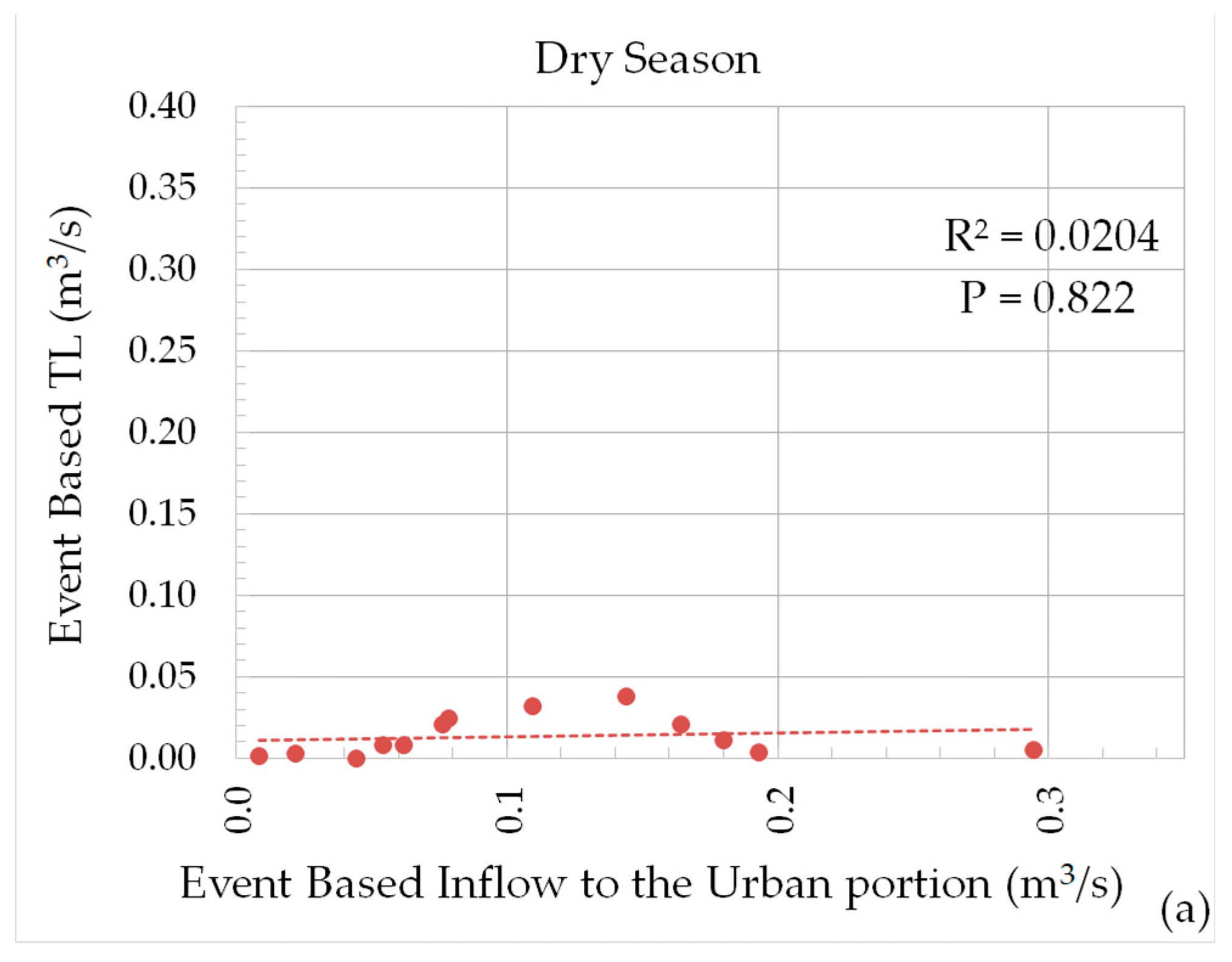
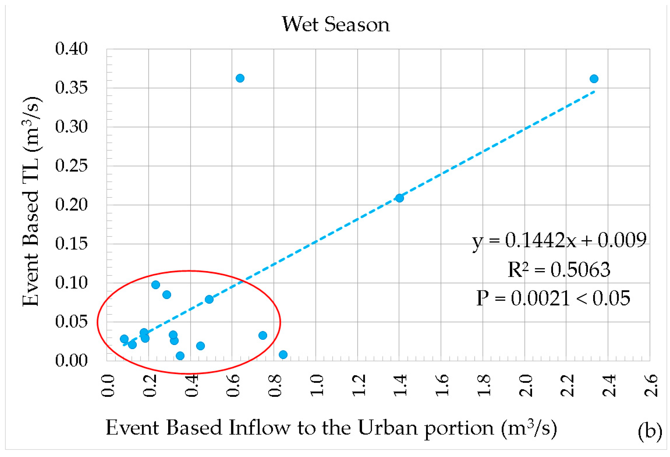
The average annual TL for the urban channel is 0.054 m3/s and reduces the urban flow by 5.7%. Figure 6 shows how TL varies with the average inflow of the urban downstream portion based on the storm events selected in the dry season (November to May) and wet season (June to October). There is no correlation between the inflow and TL of the event selected from the dry season. Figure 6a shows that the average TL of an event is negligible at 0.01 m3/s. So, it can be concluded that TL is not required to consider the events occurring in the dry season. However, a relatively strong linear correlation between inflow and TL can be observed for the storm event during the wet season (Figure 6b). However, still, the average TL is around 0.04 m3/s for the wet seasonal storm events that had generated inflow less than or equal to 0.8 m3/s. So, the TL of the wet seasonal events can be categorised into two zones. If the inflow of a storm event is greater than 0.8 m3/s, then TL can be estimated using TL = 0.1442 × Inflow + 0.009. The main reason for this better correlation between inflow and TL during wet seasonal events is the higher wetted perimeter flow, leading to high TL.
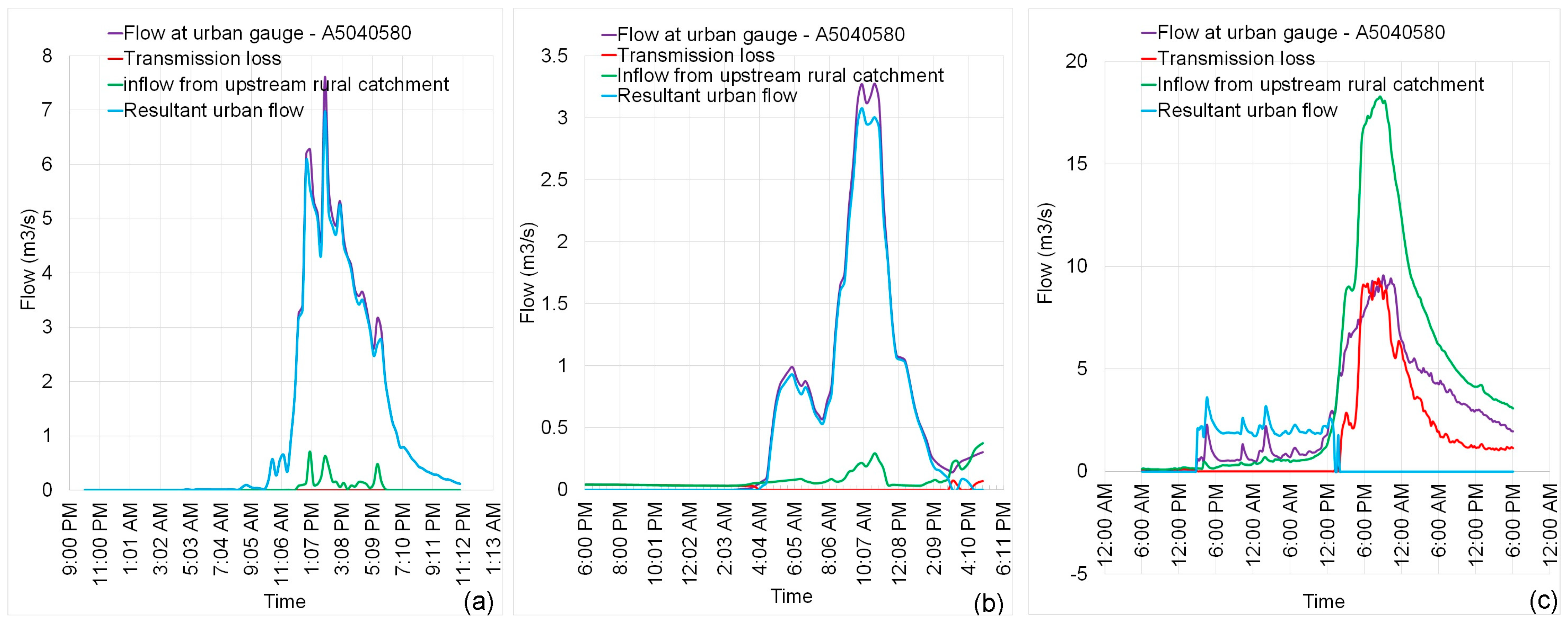
This study uses a relatively simple TL calculation introduced by McMahon, et al. [39] based on the continuity of the catchment flow mass balance. Figure 7 shows the three different runoff events from the urban portion and the resultant urban flow after considering the TL. The estimated TL in Figure 7a,b (based on U17 and U1of Table 3) was small, and this was the general flow observation in the urban portion of the BHC. However, the estimated average TL (1.65 m3/s) of the event shown in Figure 7c (event on 13/09/2016) was much higher than that of the events in Figure 7a,b. This was because the recorded inflow was significantly higher than the outflow observed at the downstream urban gauge station. If this observation was not due to an error in data recording or the rating curve, another possibility is the unaccounted outflow from the rural portion flow before it reaches the downstream urban gauge station. Figure 7c represents a big event, and there is a chance of flowing upper catchment (rural portion) inflow out into the low-lying areas beyond the channel. Hence, the effective inflow for estimating TL should be less than the observed inflow. However, getting an accurate inflow estimate is a challenge. As a result, this type of outlier event was removed from the loss analysis in this study, which could affect the estimated TL value for the catchment. In a separate analysis, Teoh [38] estimated a much higher daily average channel TL in Brownhill Creek up to 5 Ml/d (1.39 m3/s), based on the correlation between flows measured at the upstream rural gauge and downstream urban gauge using continuous five years hourly flow data. Though the loss estimation methods in both the studies are the same, the difference in input data, including data resolution and continuous versus event-based made a notable difference in the results. Potentially, the estimated TL in this study provides better results because it used shorter time steps (15 min) and event-based for an extended data period (25 years). As detailed in Section 1, other methods are available to estimate TL. As such, further investigation based on another method and when extensive data are available could verify this result for the BHC study area.
3.5. Challenges of Estimating Losses
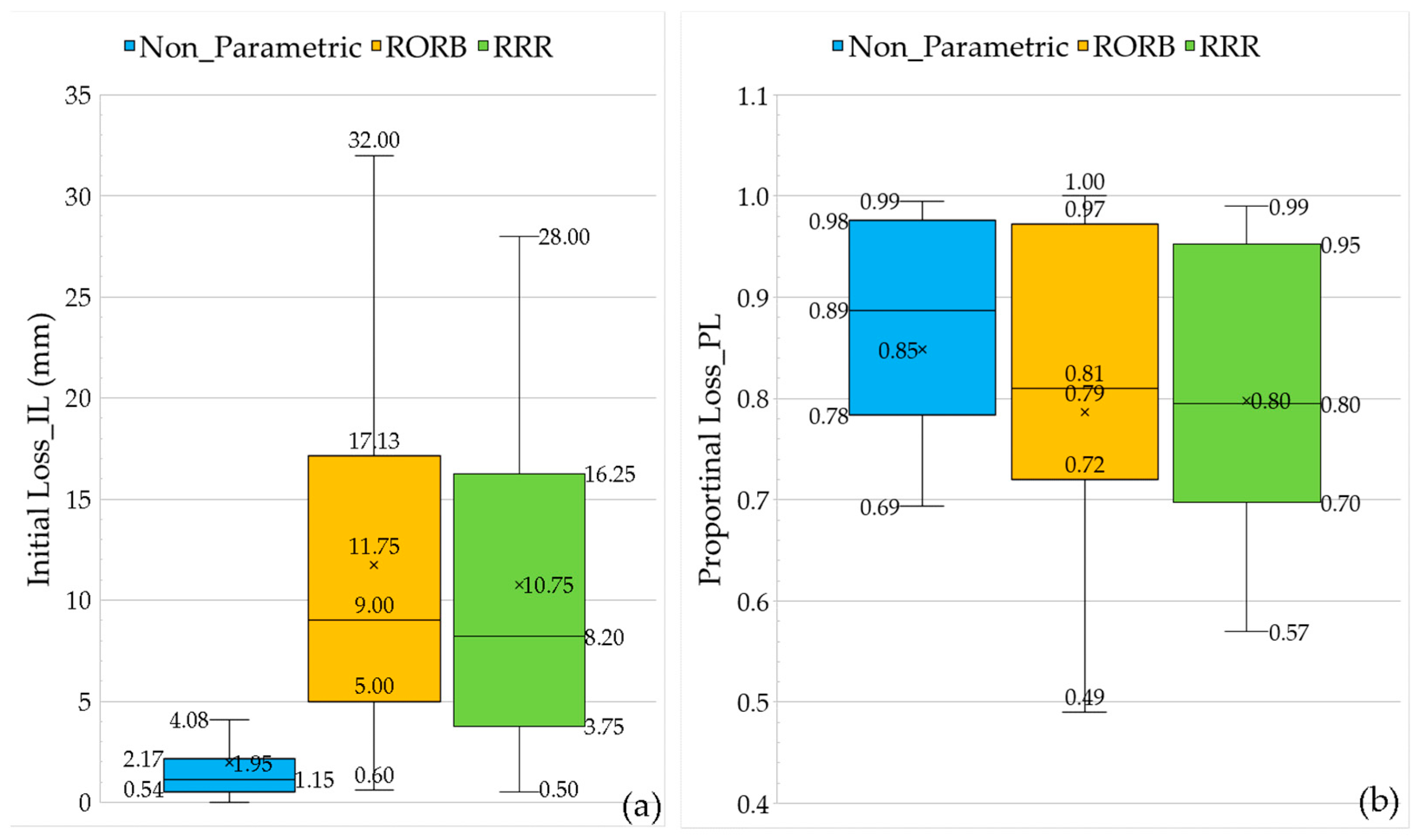
The statistical analysis of IL and PL values obtained from non-parametric (water balance) and parametric methods (RORB and RRR) for the BHC upper catchment (rural portion) are shown using boxplots in Figure 8. The results show that the median IL from all three methods is between 1.15 mm and 9 mm. However, these values are considerably low when compared with the previously estimated IL values for rural catchments in SA. For example, Gamage et al. [20] estimated mean IL between 7.9 mm and 17.2 mm for six rural catchments in SA, while Hill et al. [5] used four rural catchments and obtained IL between 15 mm to 25 mm. One reason for these differing findings is the storm event selection process differences, as noted earlier in Section 2.2.1. The focus of this study was to quantify losses for a flash flood catchment. Hence, our selection was based on including high-intensity storm events. In addition, any storm events that did not produce runoff were not chosen. Therefore, the estimated loss values were biased towards the wet antecedent conditions and highly likely to have lower loss values as found by Hill et al. [21].
The non-parametric approach of loss estimation is highly subjective to the catchment characteristics and the shape of the hydrograph [5]. Hill et al. [5] further described that the start of the hydrograph rise generally reflects the runoff from the catchment area close to the gauge station and does not indicate the runoff from upper catchment areas due to different time of concentration. In addition, the point of runoff commencement depends on data resolution and human judgment. Therefore, the non-parametric method may underestimate the potential IL values for our rural portion. As pointed out, the upper and the lower limits of the IL values estimated for the rural portion (0 mm–4.08 mm) using the non-parametric method are relatively low compared to past studies [5,20]. In this analysis, the variation of IL based on the non-parametric method was only between 0 mm and 4.08 mm. So, confidence in using the non-parametric method to estimate rural losses for similar catchments is low.
The loss values obtained from the RORB model are based on the pervious areas. As a result, RORB estimates losses better in the rural catchments [5,27,73]. The catchment area of the rural portion of the BHC study area is about 92%, hence the estimated median IL value of 9 mm using the RORB model can be a good representation of the potential losses for our rural portion. However, the results in Figure 8 highlighted that the observed IL and PL values based on the RORB model have a high range across the selected rainfall events (0.6 < IL (mm) < 32 and 0.49 < PL < 1).
The statistics summary of the losses based on the RRR model in Figure 8 shows that the median IL for the rural portion was 8.2 mm, and PL was 0.8. Though the PL values obtained from RORB and RRR are close, the IL values obtained by the two models reveal that the mean values from RORB are 9% higher than that of the RRR method. One reason for this difference may be that RORB allows for spatial variability in rainfall across the catchment through sub-areas, but the RRR model uses average rainfall in a single catchment [28]. In addition, the RRR model uses the total catchment area for loss calculation, while RORB uses only the pervious area. Thus, the IL values obtained from the RORB model are more advanced for the rural portion.
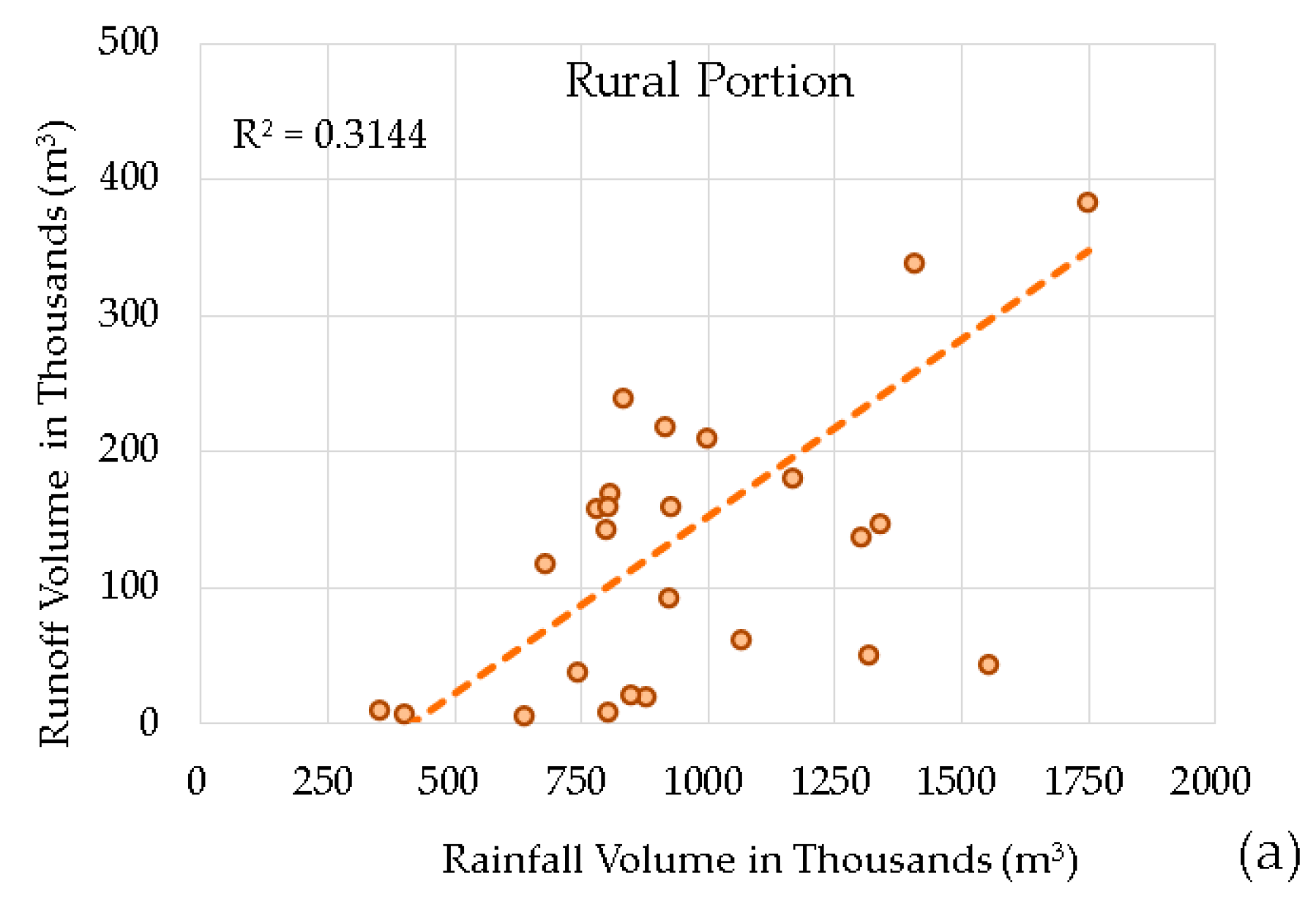
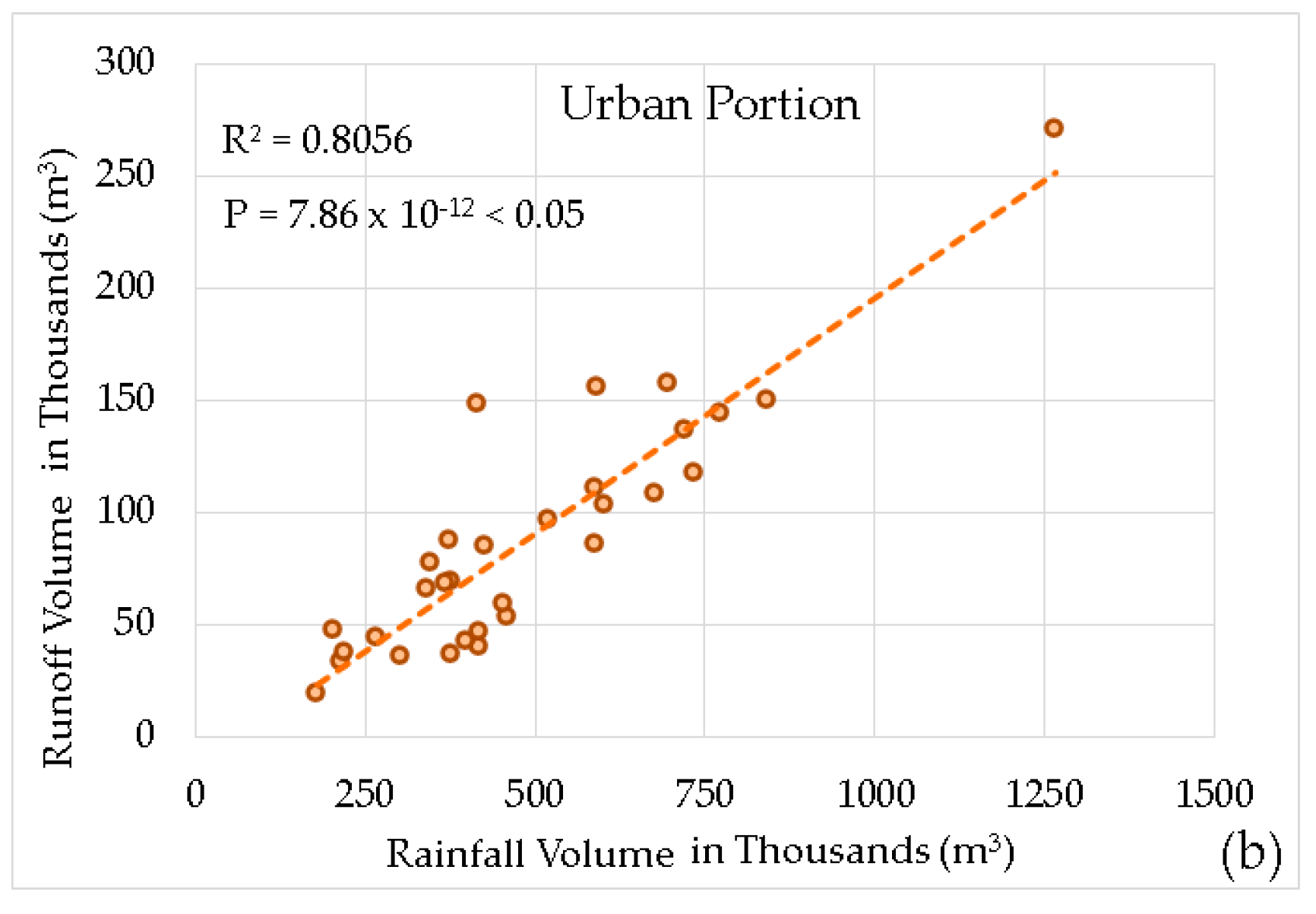
Based on the rainfall and runoff volume comparison (Figure 9a), there is a poor linear relationship with R2 (0.3144) and low p value (0.0029). This suggests that the relationship does not explain much of variation of the data, but it is statistically significant. This is expected as the rainfall-runoff process of a natural catchment is non-linear due to the storage effect of the soil sub-surface and other factors, such as antecedent wetness and vegetative cover, that significantly influence losses and runoff. On the other hand, a relatively strong linear relationship between rainfall and runoff volume with R2 (0.806) and P value (7.86 × 10⁻¹²) was observed for the urban portion of the study area (Figure 9b). This means that the runoff contribution of each selected event for the urban portion is almost in proportion to the rainfall volume and has little effect on the other factors. Thus, it can be concluded that the runoff contribution of each event is mainly from EIA, with no contribution from unconnected areas in the urban portion. Therefore, some challenges need to be addressed when estimating IL values using the selected methods because each method interprets losses differently for the urban portion and provides different results.
With a little modification to the catchment file, as detailed in Section 2.2.6, the RORB model can treat EIA and unconnected areas separately when calculating losses for the urban portion. The challenge is that when there is no runoff contribution from the unconnected areas, RORB cannot calculate losses. As detailed above, the unconnected area contribution of the urban portion of the BHC study area is negligible for most of the selected events. Therefore, the RORB model cannot estimate losses for the urban portion. On the other hand, the RRR model used the entire area of the urban portion for loss estimation and could not distinguish between EIA and unconnected areas separately. As a result, the estimated IL values from the RRR did not reflect the actual loss of either the unconnected areas or EIA. With these observations, we can conclude that the loss values obtained from parametric methods did not reflect the actual loss of the urban portion.
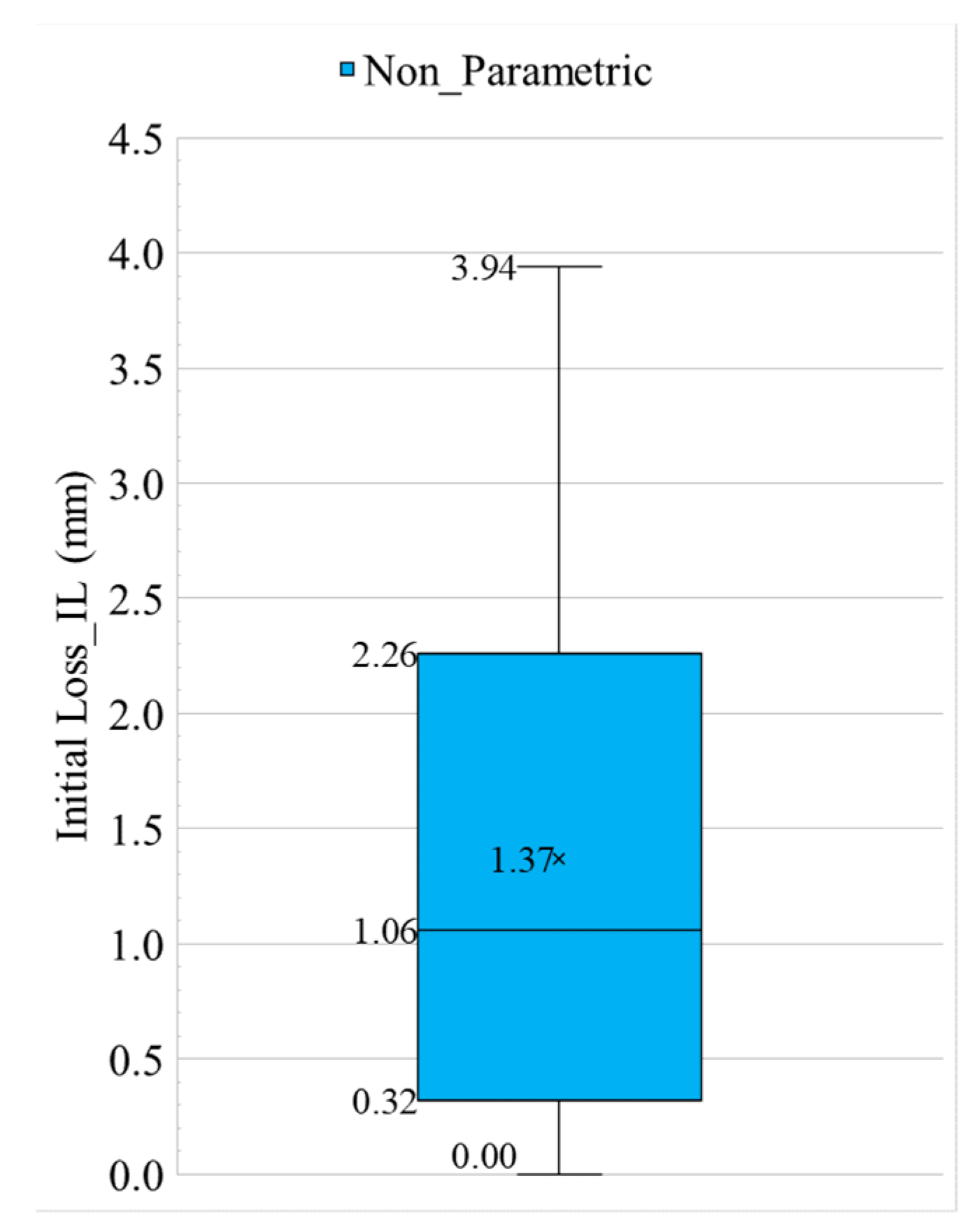
The non-parametric method provided different loss values for the urban portion. The start of the hydrograph rise reflects the runoff from the area with a quick response time which is generally from the EIA of the urban portion. Therefore, the IL of the urban portion estimated using the non-parametric method shown in Figure 10 (mean and median are 1.37 mm and 1.06 mm) can be considered as the IL of the EIA. However, there are no studies performed in SA to validate IL of EIA of the urban areas, but this finding goes along with the ARR 2016 recommendation that the IL values for the EIA should be between 1–2 mm [8]. This finding is still valid for the urban catchments that produce runoff mainly from EIA. Because the runoff contributes only from EIA in the urban portion, PL is not a proportional loss on the EIA but reflects the percentage of EIA. However, it should be noted that these findings are not valid when the runoff contribution exists from both EIA and unconnected areas of an urban catchment. If that is the scenario, the IL estimation based on the non-parametric method will be higher as it represents the IL from unconnected areas as well.
This section discusses a few critical challenges faced during the loss estimating process conducted for the partly urbanised Brownhill Creek catchment in the Adelaide metropolitan region in SA. The challenges were mainly found when selecting the rainfall events, the storm event’s time resolution, and the most appropriate loss estimation method. In addition, extracting baseflow using the Lyne and Hollick algorithm and estimating transmission losses were also challenged for the selected events because of some data limitations. Further, this section provides some strategies that can be used to minimise the adverse effects of these challenges with the available resources.
However, it is always challenging to have adequate intense rainfall events with low AEP floods for an urban catchment in the Mediterranean climate. As a result, obtaining a representative loss estimation for flash flood forecasting systems is challenging. On the other hand, most of the other challenges, mainly the IL estimation of urban portions of the catchment and baseflow separation, can be improved if the selected rainfall-runoff model is a multi-process model.
4. Conclusions
This study explores the challenges when determining IL and PL values of the partly urbanised BHC catchment using the runoff generated low AEP rainfall events. The following conclusions can be drawn:
- The selection of an appropriate method of estimating losses is critical to obtaining reliable IL and PL values in a partly urbanised catchment. The parametric methods based on a rainfall-routing model, such as RORB and RRR, can overcome some challenges attached to the non-parametric method and provide more accurate loss estimation for the rural portion of the BHC catchment.
- The mean IL values estimated for the rural portion using the RORB model were 9% higher than that of the RRR model. This is mainly because the RORB model uses spatial variability in rainfall through sub-areas and applies only to the unconnected areas, 92% of the total. However, the RRR model used average rainfall for the whole catchment.
- The loss estimations are based on the runoff generated by mainly the low AEP rainfall events. Hence, the estimated loss values are biased towards wet antecedent conditions, and lower loss values can be observed. The recommended median IL and PL are 9 mm and 0.79 respectively for the rural portion of the study area, estimated using the RORB model.
- The loss values estimated for the urban portion were slightly different as it was necessary to assess losses from EIA (23% of the catchment area) and unconnected areas separately. The RORB model generally provides losses of unconnected areas. Therefore, a minor modification to the catchment file was done by breaking each sub-area into two parts to assign separate EIA and unconnected areas. Still, RORB did not estimate the losses of the unconnected areas of the urban portion as the catchment response to the rainfall events is mainly from EIA and runoff contribution did not exist in unconnected areas. Hence, the RORB model cannot be used to extract the representative loss values of the event selected for the urban portion. Similarly, the simple RRR model used in this study does not discriminate the runoff from EIA and unconnected areas. Hence, it also did not provide the representative loss values for the urban portion.
- IL estimated from the non-parametric method can be considered as IL of EIA of the urban portion. The estimated mean and median IL were around 1.37 mm and 1.06 mm, respectively. However, this finding is not valid for the catchment where the runoff contribution exists from EIA and unconnected areas.
- Though 19 storm events were found to be at 20% AEP or less since 1993, only eight events had 20% AEP or less resulting flow. So, a few more storm events with higher AEP (up to 63.5% AEP) were selected for the completeness of the study. Therefore, the estimated losses may not accurately represent the losses of the flash flood events.
- TL was observed at the channel in the urban portion of the study area and the continuity of the catchment flow mass balance was used to estimate TL. Some outlier events, potentially due to possible errors in data, challenged the average annual TL, 0.054 m3/s. A higher average TL of 0.14 m3/s was estimated for the wet season mainly because of the higher unaccounted outflow into the low-lying area adjacent to the channel. However, TL can be considered as 0.04 m3/s when the inflow is less than 0.8 m3/s and otherwise, using TL = 0.1442 × Inflow + 0.009. The TL of the dry seasonal events were between 0 and 0.04 m3/s. When extensive data are available, further investigations are recommended to review the TL estimations.
- A 15-min temporal resolution of rainfall and flow data was used to obtain losses in this study. However, to obtain better outcomes, it is recommended to use data with even shorter time steps, such as 10- or 5-min temporal resolution.
Baseflow separation was performed for the events selected in the upper rural portion adopting the widely used Lyne and Holick filter method. Though 15-min temporal resolution data were used, the recession constant used for the filter method was 0.925, which is generally used for the 1-h time step. If the appropriate recession constant for 15-min time steps can be used, a better output can be obtained. In addition, baseflow was not separated from the events selected from the urban portion as the catchment response did not show any baseflow. So, careful analysis of catchment specific conditions is required before starting the flow calculation. This leads to determining the catchment-specific flow values, which is critical for estimating the losses.
Author Contributions
Conceptualization, D.C.R., G.A.H. and D.J.K.; methodology, D.C.R., G.A.H. and D.J.K.; software, D.C.R. and D.J.K.; validation, D.C.R., G.A.H. and D.J.K.; formal analysis, D.C.R.; investigation, D.C.R.; resources, D.C.R. and G.A.H.; data curation, D.C.R.; writing—original draft preparation, D.C.R.; writing—review and editing, D.C.R., G.A.H. and D.J.K.; supervision, G.A.H. and D.J.K.; project administration, D.C.R. and G.A.H.; funding acquisition, G.A.H. All authors have read and agreed to the published version of the manuscript.
Funding
This research is funded by the University of South Australia through postgraduate scholarship award scheme named Research Training Program-Domestic (RTPd).
Institutional Review Board Statement
Not applicable.
Informed Consent Statement
Not applicable.
Data Availability Statement
Not applicable.
Acknowledgments
The authors acknowledge all participants for their time and effort. Further, they would like to express their gratitude to the Department for Environment and Water, Bureau of Meteorology, and Water Data Services Pty Ltd. in Adelaide for providing the extensive data.
Conflicts of Interest
The authors declare no conflict of interest.
References
- Ball, J.; Babister, M.; Nathan, R.; Weeks, W.; Weinmann, E.; Retallick, M.; Testoni, I. Australian Rainfall and Runoff: A Guide to Flood Estimation; Commonwealth of Australia (Geoscience Australia): Barton, Australia, 2019. Available online: http://hdl.handle.net/10453/85297 (accessed on 22 November 2021).
- Hill, P.I.; Mein, R.G.; Siriwardena, L. How Much Rainfall Becomes Runoff? Loss Modelling for Flood Estimation; Cooperative Research Centre for Catchment Hydrology, Monash University: Clayton, Australia, 1998. [Google Scholar]
- Ramier, D.; Berthier, E.; Andrieu, H. The hydrological behaviour of urban streets: Long-term observations and modelling of runoff losses and rainfall–runoff transformation. Hydrol. Process. Int. J. 2011, 25, 2161–2178. [Google Scholar] [CrossRef]
- El-Kafagee, M.; Rahman, A. A study on initial and continuing losses for design flood estimation in new south wales. In Proceedings of the 19th International Congress on Modelling and Simulation, MODSIM, Perth, Australia, 12–16 December 2011; pp. 12–16. [Google Scholar]
- Hill, P.; Graszkiewicz, Z.; Taylor, M.; Nathan, R. Australian rainfall and runoff revision project 6: Loss models for catchment simulation: Phase 4 analysis of rural catchments. Aust. Barton ACT 2014. Available online: https://arr.ga.gov.au/__data/assets/pdf_file/0005/40496/ARR_Project6_Phase-4_Report.pdf (accessed on 12 November 2021).
- Lang, S.; Hill, P.; Scorah, M.; Stephens, D. Defining and calculating continuing loss for flood estimation. In 36th Hydrology and Water Resources Symposium: The Art and Science of Water; Simon, L., Hill, P., Scorah, M., Stephens, D., Eds.; Engineers Australia: Barton, Australia, 2015; p. 193. [Google Scholar]
- Tularam, G.A.; Ilahee, M. Initial loss estimates for tropical catchments of australia. Environ. Impact Assess. Rev. 2007, 27, 493–504. [Google Scholar] [CrossRef]
- Phillips, B.; Goyen, A.; Thomson, R.; Pathiraja, S.; Pomeroy, L. Loss Models for Catchment Simulation—Urban Catchments; Engineers Australia: Barton, Australia, 2014; p. 165. [Google Scholar]
- Ebrahimian, A.; Wilson, B.N.; Gulliver, J.S. Improved methods to estimate the effective impervious area in urban catchments using rainfall-runoff data. J. Hydrol. 2016, 536, 109–118. [Google Scholar] [CrossRef]
- Hill, P.; Thomson, R. Losses, book 5: Flood hydrograph estimation. In Australian Rainfall and Runoff–A Guide to Flood Estimation; Commonwealth of Australia: Barton, Australia, 2019. [Google Scholar]
- Schoener, G.; Stone, M.C.; Thomas, C. Comparison of seven simple loss models for runoff prediction at the plot, hillslope and catchment scale in the semiarid southwestern us. J. Hydrol. 2021, 598, 126490. [Google Scholar] [CrossRef]
- Vafakhah, M.; Nikche, A.F.; Sadeghi, S.H. Comparative effectiveness of different infiltration models in estimation of watershed flood hydrograph. Paddy Water Environ. 2018, 16, 411–424. [Google Scholar] [CrossRef]
- Borah, D.K. Hydrologic procedures of storm event watershed models: A comprehensive review and comparison. Hydrol. Process. 2011, 25, 3472–3489. [Google Scholar] [CrossRef]
- David, J.S.; Valente, F.; Gash, J.H. Evaporation of intercepted rainfall. Encycl. Hydrol. Sci. 2006. [Google Scholar] [CrossRef]
- Nandakumar, N.; Mein, R. Calibration of a rainfall-runoff model for forested and pastured catchments. In Water Down Under 94: Surface Hydrology and Water Resources Papers; Institution of Engineers: Barton, Australia, 1994; p. 481. [Google Scholar]
- Ilahee, M.; Imteaz, M.A. Improved continuing losses estimation using initial loss-continuing. Am. J. Engg. Appl. Sci. 2009, 2, 796–803. [Google Scholar]
- Loveridge, M.; Rahman, A.; Hill, P. Applicability of a physically based soil water model (swmod) in design flood estimation in eastern australia. Hydrol. Res. 2016, 48, 1652–1665. [Google Scholar] [CrossRef] [Green Version]
- Sahu, R.; Mishra, S.; Eldho, T.; Jain, M. An advanced soil moisture accounting procedure for scs curve number method. Hydrol. Process. Int. J. 2007, 21, 2872–2881. [Google Scholar] [CrossRef]
- Ahmad, I.; Verma, V.; Verma, M.K. Application of curve number method for estimation of runoff potential in gis environment. In 2nd International Conference on Geological and Civil Engineering; IACSIT Press: Singapore, 2015; pp. 16–20. [Google Scholar] [CrossRef]
- Gamage, S.; Hewa, G.; Beecham, S. Modelling hydrological losses for varying rainfall and moisture conditions in south australian catchments. J. Hydrol. Reg. Stud. 2015, 4, 1–21. [Google Scholar] [CrossRef] [Green Version]
- Hill, P.; Graszkiewicz, Z.; Loveridge, M.; Nathan, R.; Scorah, M. Analysis of loss values for australian rural catchments to underpin arr guidance. In 36th Hydrology and Water Resources Symposium: The Art and Science of Water; Hill, P., Graszkiewicz, Z., Loveridge, M., Nathan, R., Scorah, M., Eds.; Engineers Australia: Barton, Australia, 2015; p. 72. [Google Scholar]
- Dyer, B.; Nathan, R.; McMahon, T.; O′Neill, I. Development of regional prediction equations for the rorb runoff routing model. Coop. Res. Cent. Catchment Hydrol. Rep. 1994, 94, 93. [Google Scholar]
- Goyen, A.G. Spatial and Temporal Effects on Urban Rainfall/Runoff Modelling. Ph.D. Thesis, Faculty of Engineering, University of Technology, Sydney, Australia, 2000. [Google Scholar]
- Laurenson, E.; Mein, R.; Nathan, R. User manual of rorb version 6, runoff routing program. 2010. Available online: https://www.monash.edu/engineering/departments/civil/research/themes/water/rorb (accessed on 15 September 2021).
- Ilahee, M. Modelling Losses in Flood Estimation. Ph.D. Thesis, Queensland University of Technology, Brisbane, Australia, 2005. [Google Scholar]
- Rahman, A.; El-Kafagee, M.; Haque, M. Derivation of improved initial and continuing losses in design flood estimation for nsw australia. J. Hydrol. Environ. Res. 2016, 4, 18–24. Available online: http://jher.org/archive/vol4/Rahman-offprint-Final-1.pdf (accessed on 25 October 2021).
- Kemp, D.; Daniell, T. A review of flow estimation by runoff routing in australia–and the way forward. Aust. J. Water Resour. 2020, 24, 139–152. [Google Scholar] [CrossRef]
- Kemp, D. The Development of a Rainfall-Runoff-Routing (rrr) Model. Ph.D. Thesis, University of Adelaide, Adelaide, Australia, 2002. [Google Scholar]
- Carroll, D. Urbs–A Catchment Runoff Routing and Flood Forecasting Model; Queensland Department of Natural Resources: Brisbane, Australia, 2001; p. 130. [Google Scholar]
- Boyd, M.; Bufill, M.; Knee, R. Pervious and impervious runoff in urban catchments. Hydrol. Sci. J. 1993, 38, 463–478. [Google Scholar] [CrossRef]
- Milevski, P. Determining the Parameters of the Flood Hydrograph Model Wbnm for Urban Catchments. Ph.D. Thesis, University of Wollongong, Wollongong, Australia, 1998. [Google Scholar]
- Pate, H.; Rahman, A. Design flood estimation using monte carlo simulation and rorb model: Stochastic nature of rorb model parameters. In World Environmental and Water Resources Congress 2010: Challenges of Change; Pate, H., Rahman, A., Eds.; ASCE Press: Reston, VA, USA, 2010; pp. 4692–4701. [Google Scholar]
- Schoener, G.J.J.o.H.E. Quantifying transmission losses in a new mexico ephemeral stream: A losing proposition. J. Hydrol. Eng. 2017, 22, 05016038. [Google Scholar] [CrossRef] [Green Version]
- Shanafield, M.; Cook, P.G. Transmission losses, infiltration and groundwater recharge through ephemeral and intermittent streambeds: A review of applied methods. J. Hydrol. 2014, 511, 518–529. [Google Scholar] [CrossRef]
- Cataldo, J.; Behr, C.; Montalto, F.; Pierce, R. A summary of published reports of transmission losses in ephemeral streams in the us. Natl. Cent. Hous. Environ. 2004, 42, 28–29. [Google Scholar]
- Cataldo, J.C.; Behr, C.; Montalto, F.A.; Pierce, R.J. Prediction of transmission losses in ephemeral streams, western USA. Open Hydrol. J. 2010, 9, 19–34. [Google Scholar] [CrossRef] [Green Version]
- Sharma, K.; Murthy, J. Estimating transmission losses in an arid region. J. Arid. Environ. 1994, 26, 209–219. [Google Scholar] [CrossRef]
- Teoh, K. Assessment of Surface Water Resources of Patawalonga Catchment and the Impact of Farm Dam Development; Department of Water, Land and Biodiversity Conservation: Adelaide, Australia, 2006. [Google Scholar]
- McMahon, T.A.; Nathan, R.J. Baseflow and transmission loss: A review. Water 2021, 8, e1527. [Google Scholar] [CrossRef]
- Jovanovic, B.; Jones, D.A.; Collins, D.J. A high-quality monthly pan evaporation dataset for australia. Clim. Chang. 2008, 87, 517–535. [Google Scholar] [CrossRef]
- McMillan, H.K.; Westerberg, I.K.; Krueger, T. Hydrological data uncertainty and its implications. Wires Water 2018, 5, e1319. [Google Scholar] [CrossRef] [Green Version]
- Gao, C.; Xu, Y.-P.; Zhu, Q.; Bai, Z.; Liu, L. Stochastic generation of daily rainfall events: A single-site rainfall model with copula-based joint simulation of rainfall characteristics and classification and simulation of rainfall patterns. J. Hydrol. 2018, 564, 41–58. [Google Scholar] [CrossRef]
- Corral, C.; Berenguer, M.; Sempere-Torres, D.; Poletti, L.; Silvestro, F.; Rebora, N. Comparison of two early warning systems for regional flash flood hazard forecasting. J. Hydrol. 2019, 572, 603–619. [Google Scholar] [CrossRef] [Green Version]
- Halgamuge, M.N.; Nirmalathas, A. Analysis of large flood events: Based on flood data during 1985–2016 in australia and india. Int. J. Disaster Risk Reduct. 2017, 24, 1–11. [Google Scholar] [CrossRef]
- Kemp, D.; Lipp, W.R. Predicting Storm Runoff in Adelaide—What Do We Know? Transport SA: Adelaide, Austalia, 1999. [Google Scholar]
- Fuller, J.; Gomez, M.; McLean, A.; Fisher, G. Channel Capacity Assessment, Brownhill Keswick and Keswick Creek Survey and Hydraulic Assessment; Australian Water Environments: Adelaide, Australia, 2012.
- Dillon, P.; Bellchambers, R.; Meyer, W.; Ellis, R. Community perspective on consultation on urban stormwater management: Lessons from brownhill creek, south australia. Water 2016, 8, 170. [Google Scholar] [CrossRef] [Green Version]
- Rahman, A.; Weinmann, P.E.; Hoang, T.M.T.; Laurenson, E.M. Monte carlo simulation of flood frequency curves from rainfall. J. Hydrol. 2002, 256, 196–210. [Google Scholar] [CrossRef]
- Graszkiewicz, Z.; Murphy, R.; Hill, P.; Nathan, R. Review of techniques for estimating the contribution of baseflow to flood hydrographs. In Proceedings of the 34th World Congress of the International Association for Hydro-Environment Research and Engineering: 33rd Hydrology and Water Resources Symposium and 10th Conference on Hydraulics in Water Engineering; Graszkiewicz, Z., Murphy, R., Hill, P., Nathan, R., Eds.; Engineers Australia: Barton, Australia, 2011; p. 138. [Google Scholar]
- Arnold, J.; Allen, P.; Muttiah, R.; Bernhardt, G.J.G. Automated base flow separation and recession analysis techniques. Groundwater 1995, 33, 1010–1018. [Google Scholar] [CrossRef]
- Tan, S.B.; Lo, E.Y.-M.; Shuy, E.B.; Chua, L.H.; Lim, W.H.J.J.o.H.E. Hydrograph separation and development of empirical relationships using single-parameter digital filters. J. Hydrol. Eng. 2009, 14, 271–279. [Google Scholar] [CrossRef]
- Latuamury, B.; Osok, R.M.; Puturuhu, F.; Imlabla, W.N. Baseflow separation using graphic method of recursive digital filter on wae batu gajah watershed, ambon city, maluku. In IOP Conference Series: Earth and Environmental Science; IOP Publishing: Bristol, UK, 2022; p. 012028. [Google Scholar]
- Chapman, T.; Maxwell, I. Baseflow separation-comparison of numerical methods with tracer experiments. In National Conference Publication-Institution of Engineers Australia NCP; Institution of Engineers, Australia: Barton, Australia, 1996; pp. 539–546. [Google Scholar]
- Zhang, J.; Zhang, Y.; Song, J.; Cheng, L. Evaluating relative merits of four baseflow separation methods in eastern australia. J. Hydrol. 2017, 549, 252–263. [Google Scholar] [CrossRef]
- Kang, T.; Lee, S.; Lee, N.; Jin, Y. Baseflow separation using the digital filter method: Review and sensitivity analysis. Water 2022, 14, 485. [Google Scholar] [CrossRef]
- Lyne, V.; Hollick, M. Stochastic time-variable rainfall-runoff modelling. In Institute of Engineers Australia National Conference; Lyne, V., Hollick, M., Eds.; Institute of Engineers, Australia: Barton, Australia, 1979; pp. 89–93. [Google Scholar]
- Eckhardt, K. How to construct recursive digital filters for baseflow separation. Hydrol. Process. Int. J. 2005, 19, 507–515. [Google Scholar] [CrossRef]
- Ladson, A.; Brown, R.; Neal, B.; Nathan, R. A standard approach to baseflow separation using the lyne and hollick filter. Australas. J. Water Resour. 2013, 17, 25–34. [Google Scholar] [CrossRef]
- Evans, R.; Neal, B. Baseflow Analysis as a Tool for Groundwater–Surface Water Interaction Assessment; Sinclair Knight Merz: Victoria, Australia, 2005; Available online: http://www.insidecotton.com/jspui/bitstream/1/1796/2/pr071282.pdf (accessed on 18 December 2021).
- Rachel, M.; Zuzanna, G.; Peter, H.; Brad, N.; Rory, N.; Tony, L. Project 7: Baseflow for Catchment Simulation; Australian Rainfall and Runoff: Barton, Australia, 2009.
- Brown, R.; Graszkiewicz, Z.; Hill, P.; Neal, B.; Nathan, R. Predicting baseflow contributions to design flood events in Australia. In Proceedings of the 34th World Congress of the International Association for Hydro-Environment Research and Engineering: 33rd Hydrology and Water Resources Symposium and 10th Conference on Hydraulics in Water Engineering; Brown, R., Graszkiewicz, Z., Hill, P., Neal, B., Nathan, R., Eds.; Engineers Australia: Barton, Australia, 2011; p. 64. Available online: https://search.informit.org/doi/10.3316/informit.263894067353773 (accessed on 10 October 2021).
- Kemp, D. Brown Hill Creek Hydrology Review; Patawalonga Catchment Water Management Board: Adelaide, Australia, 1998.
- Bhaskar, N.R.; French, M.N.; Kyiamah, G.K. Characterization of flash floods in eastern kentucky. J. Hydrol. Eng. 2000, 5, 327–331. [Google Scholar] [CrossRef]
- Smythe, C.; Newell, G.; Druery, C. Flood Forecast Mapping Sans Modelling; Smythe, C., Newell, G., Druery, C., Eds.; Floodplain Management Association National Conference: Brisbane, Australia, 2015. [Google Scholar]
- Wasko, C.; Shao, Y.; Vogel, E.; Wilson, L.; Wang, Q.; Frost, A.; Donnelly, C. Understanding trends in hydrologic extremes across australia. J. Hydrol. 2021, 593, 125877. [Google Scholar] [CrossRef]
- Wenger, C.; Hussey, K.; Pittock, J. Living with Floods: Key Lessons from Australia and Abroad; National Climate Change Adaption Research Facility: Southport, Australia, 2013; Available online: http://hdl.handle.net/1885/65474 (accessed on 18 December 2021).
- Ostrowski, M.; Bach, M.; Gamerith, V.; De Simone, S. Analysis of the Time-Step Dependency of Parameters in Conceptual Hydrological Models; Institute of Engineering Hydrology and Water Management: Darmstadt, Germany, 2010. [Google Scholar]
- Notaro, V.; Fontanazza, C.M.; Freni, G.; Puleo, V. Impact of rainfall data resolution in time and space on the urban flooding evaluation. Water Sci. Technol. 2013, 68, 1984–1993. [Google Scholar] [CrossRef] [Green Version]
- Bastola, S.; Murphy, C. Sensitivity of the performance of a conceptual rainfall–runoff model to the temporal sampling of calibration data. Hydrol. Res. 2013, 44, 484–494. [Google Scholar] [CrossRef]
- Lyu, H.; Ni, G.; Cao, X.; Ma, Y.; Tian, F. Effect of temporal resolution of rainfall on simulation of urban flood processes. Water 2018, 10, 880. [Google Scholar] [CrossRef] [Green Version]
- Huang, Y.; Bárdossy, A.; Zhang, K. Sensitivity of hydrological models to temporal and spatial resolutions of rainfall data. Hydrol. Earth Syst. Sci. 2019, 23, 2647–2663. [Google Scholar] [CrossRef] [Green Version]
- Ficchì, A.; Perrin, C.; Andréassian, V. Impact of temporal resolution of inputs on hydrological model performance: An analysis based on 2400 flood events. J. Hydrol. 2016, 538, 454–470. [Google Scholar] [CrossRef]
- Pearcey, M.; Pettett, S.; Cheng, S.; Knoesen, D. Estimation of rorb kc parameter for ungauged catchments in the pilbara region of western australia. In Hydrology and Water Resources Symposium 2014; Pearcey, M., Pettett, S., Cheng, S., Knoesen, D., Eds.; Engineers Australia: Barton, Australia, 2014; p. 206. [Google Scholar]
Figure 1.
Study Area.

Figure 2.
BHC catchment (a) Gauging stations and (b) Average annual rainfall comparison.

Figure 3.
Approach of estimating IL and PL for the BHC catchment.

Figure 4.
Thiessen polygon area and weights for the BHC catchment.

Figure 5.
IL-PL Loss Models (Source: Section 3.2.3, ARR Book 5, Chapter 3).

Figure 6.
TL and inflow of the urban portion for (a) dry season (b) wet season.


Figure 7.
Urban flow based on event (a) U17 (b) U1 (c) 13/09/2016.

Figure 8.
Box plot of (a) IL (b) PL for rural portion.

Figure 9.
Rainfall and runoff relationships for the BHC (a) rural portion (b) urban portion.


Figure 10.
Box plot of IL based on non-parametric method for the urban portion.


Table 1.
Empirical loss models used in rainfall runoff models.
| Rainfall Runoff Model | Method | Incorporated Loss Models | References | Model Structure | Model Access |
|---|---|---|---|---|---|
| RORB-Runoff Routing for a Burroughs Computers | Non-linear storage routing | IL/CL and IL/PL | Laurenson, et al. [24] | Loss calculation based on pervious area runoff. Losses from one runoff process only (direct surface runoff). | Free |
| URBS-Unified Basin Simulator Model | Non-linear storage routing | IL/CL, IL//PL and Manley-Phillips | Carroll [29] | The URBS models rainfall losses for impervious and pervious areas separately. Losses from one runoff process only (direct surface runoff). | A license copy is required |
| WBNM-Watershed Bounded Network Model | Non-linear storage routing | IL/CL and IL/PL | Boyd, et al. [30]; Milevski [31] | The WBNM models rainfall losses for impervious and pervious areas separately. Losses from one runoff process only (direct surface runoff). | A license copy is required |
| RAFTS | Non-linear storage routing | IL/CL, IL/PL and Australian Representative Basins Model | XP Software (2009) | Loss calculation based on pervious area runoff. Losses from one runoff process only (direct surface runoff). | A license copy is required |
| RRR-Rainfall Runoff Routing | Linear channel storage and non-linear storage routing | IL/PL | Kemp [28] | Three runoff processes for rural sub-areas and two runoff processes for urban sub-areas | Not publicly available yet |
Table 2.
Criteria adopted for selection of the storm events.
| Parameter | Value Adopted | Units |
|---|---|---|
| Select event when period of no rainfall (before and after the event) [8] | 5 | hours |
| Minimum cumulative depth of rainfall [8] | 10 | mm |
Table 3.
Selected storm events.
| Event Date (Rural Portion) | Event No | Total Rainfall (mm) | Total Runoff Volume ×103 (m3) | BoM Design Rainfall AEP (%) | AEP of Flow (%) | Event Date (Urban Portion) | Event No | Total Rainfall (mm) | Total Runoff Volume ×103 (m3) | BoM Design Rainfall AEP (%) | AEP of Flow (%) |
|---|---|---|---|---|---|---|---|---|---|---|---|
| 21 July 1995 | R1 | 43.6 | 264.6 | 63.2 | 25 | 03 July 1996 | U1 | 18.4 | 51.0 | 63.2 | 80 |
| 30 October 1997 | R2 | 73.6 | 58.2 | 10 | 100 | 30 July 1996 | U2 | 25.8 | 170.7 | 63.2 | 100 |
| 07 February 1998 | R3 | 22.3 | 6.0 | 50 | 100 | 21 August 1996 | U3 | 23.5 | 201.1 | 63.2 | 65 |
| 19 April 1998 | R4 | 49.0 | 21.4 | 20 | 100 | 30 October 1997 | U4 | 86.9 | 323.6 | 5 | 90 |
| 22 Mar 2000 | R5 | 35.6 | 5.3 | 20 | 63.2 | 07 February 1998 | U5 | 20.8 | 36.7 | 50 | 55 |
| 12 May 2000 | R6 | 44.9 | 8.9 | 50 | 100 | 11 April 1998 | U6 | 50.4 | 125.0 | 50 | 80 |
| 06 September 2000 | R7 | 37.9 | 132.4 | 50 | 24 | 19 April 1998 | U7 | 41.4 | 122.1 | 20 | 60 |
| 17 October 2000 | R8 | 72.7 | 172.2 | 20 | 25 | 12 June 1999 | U8 | 28.6 | 175.1 | 63.2 | 70 |
| 06 June 2001 | R9 | 19.6 | 12.9 | 20 | 50 | 22 Mar 2000 | U9 | 31.6 | 56.6 | 20 | 65 |
| 18 May 2002 | R10 | 86.8 | 62.2 | 10 | 63.2 | 12 May 2000 | U10 | 14.8 | 38.6 | 63.2 | 75 |
| 26 June 2003 | R11 | 41.5 | 41.2 | 50 | 63.2 | 26 June 2000 | U11 | 25.7 | 118.8 | 63.2 | 65 |
| 17 May 2004 | R12 | 47.4 | 24.1 | 50 | 100 | 17 October 2000 | U12 | 53.1 | 300.6 | 20 | 65 |
| 02 August 2004 | R13 | 46.5 | 413.7 | 63.2 | 16.5 | 25 January 2001 | U13 | 28.7 | 41.5 | 5 | 24 |
| 23 October 2005 | R14 | 55.7 | 273.4 | 50 | 23 | 06 June 2001 | U14 | 25.4 | 72.9 | 50 | 20 |
| 06 November 2005 | R15 | 97.7 | 464.3 | 5 | 3 | 23 September 2001 | U15 | 29.4 | 101.5 | 63.2 | 85 |
| 24 August 2010 | R16 | 45.1 | 247.2 | 63.2 | 33 | 18 May 2002 | U16 | 57.9 | 208.0 | 20 | 55 |
| 03 September 2010 | R17 | 44.8 | 235.1 | 63.2 | 31 | 19 February 2003 | U17 | 46.6 | 117.2 | 20 | 65 |
| 20 June 2012 | R18 | 74.8 | 196.9 | 20 | 45 | 26 June 2003 | U18 | 35.8 | 135.1 | 50 | 45 |
| 31 May 2013 | R19 | 59.6 | 95.9 | 50 | 100 | 17 May 2004 | U19 | 31.3 | 81.0 | 63.2 | 85 |
| 18 July 2013 | R20 | 51.1 | 519.6 | 63.2 | 19.5 | 19 January 2005 | U20 | 25.9 | 40.9 | 50 | 55 |
| 08 July 2014 | R21 | 44.7 | 181.1 | 63.2 | 42 | 10 June 2005 | U21 | 14.0 | 57.5 | 63.2 | 20 |
| 04 July 2016 | R22 | 65.1 | 285.0 | 50 | 32 | 11 December 2008 | U22 | 28.7 | 51.1 | 63.2 | 85 |
| 13 September 2016 | R23 | 84.6 | 944.2 | 10 | 6 | 31 May 2013 | U23 | 47.9 | 230.2 | 50 | 40 |
| 28 September 2016 | R24 | 78.6 | 634.5 | 20 | 15 | 17 July 2013 | U24 | 15.1 | 43.4 | 63.2 | 85 |
| 26 December 2016 | R25 | 51.5 | 98.8 | 50 | 31 | 12 September 2013 | U25 | 23.9 | 85.3 | 63.2 | 8 |
| 17 July 2017 | R26 | 51.8 | 202.0 | 63.2 | 32 | 13 February 2014 | U26 | 40.5 | 116.6 | 20 | 21 |
| 14 February 2014 | U27 | 40.7 | 135.7 | 20 | 50 | ||||||
| 22 January 2016 | U28 | 27.4 | 48.3 | 10 | 21 | ||||||
| 28 September 2016 | U29 | 49.6 | 762.8 | 63.2 | 12 | ||||||
| 11 October 2017 | U30 | 46.16 | 67.9 | 20 | 2.5 | ||||||
| 17 May 2018 | U31 | 40.4 | 111.2 | 50 | 85 |
Note: The AEPs of the rainfall event was gathered from BOM design IFD data (http://www.bom.gov.au/water/designRainfalls/revised-ifd/, accessed on 5 January 2022) while AEPs of the resulting flow data of the events were decided using flood frequency analyses.
Publisher’s Note: MDPI stays neutral with regard to jurisdictional claims in published maps and institutional affiliations. |
© 2022 by the authors. Licensee MDPI, Basel, Switzerland. This article is an open access article distributed under the terms and conditions of the Creative Commons Attribution (CC BY) license (https://creativecommons.org/licenses/by/4.0/).
Share and Cite
MDPI and ACS Style
Ratnayake, D.C.; Hewa, G.A.; Kemp, D.J. Challenges in Quantifying Losses in a Partly Urbanised Catchment: A South Australian Case Study. Water 2022, 14, 1313. https://doi.org/10.3390/w14081313
AMA Style
Ratnayake DC, Hewa GA, Kemp DJ. Challenges in Quantifying Losses in a Partly Urbanised Catchment: A South Australian Case Study. Water. 2022; 14(8):1313. https://doi.org/10.3390/w14081313
Chicago/Turabian StyleRatnayake, Dinesh C., Guna A. Hewa, and David J. Kemp. 2022. "Challenges in Quantifying Losses in a Partly Urbanised Catchment: A South Australian Case Study" Water 14, no. 8: 1313. https://doi.org/10.3390/w14081313
Note that from the first issue of 2016, this journal uses article numbers instead of page numbers. See further details here.