
Coherent Structures at the Interface between Water Masses of Confluent Rivers


1
Institute of Continuous Media Mechanics, UB RAS, Koroleva 1, 614013 Perm, Russia
2
Mining Institute, UB RAS, Sibirskaya 78a, 614007 Perm, Russia
*
Author to whom correspondence should be addressed.
Water 2022, 14(8), 1308; https://doi.org/10.3390/w14081308
Submission received: 6 March 2022
/
Revised: 13 April 2022
/
Accepted: 14 April 2022
/
Published: 17 April 2022
(This article belongs to the Section Hydraulics and Hydrodynamics)
Abstract
:The paper presents the results of field measurements and numerical modeling of the influence of various factors on the formation of coherent structures in the confluence zone of the Sylva and Chusovaya rivers, which are dammed by the Kamskaya Hydroelectric Power Station (HPS). A characteristic feature of the measured parameters in the zone under study is that they experience both seasonal fluctuations and fluctuations of much higher frequency associated with intraday regulation of the HPS operation. These intraday fluctuations give rise to coherent structures with periodicity T~2–10 min, which manifest themselves in the fluctuations of the specific electrical conductivity of water. The flow velocity also experiences significant fluctuations with a sufficiently wide frequency spectrum, although the characteristic period of its fluctuations is less than the period of electrical conductivity fluctuations and is equal to ~1 min. In order to study the features of the formation of such structures, numerical simulation was carried out within the framework of the three-dimensional approach. Calculations were performed for a 300-meter-long stretch of the Chusovaya River, which is located downstream of the confluence of Chusovaya and Sylva rivers and is the site of the Chusovskoy water intake of Perm city. It was found that the intraday irregularity of HPS operation gives rise to the occurrence of vortex structures in this layer, leading to the temporal variation of concentration at a given point of space and the formation of the wave structure of the concentration field at different moments of time. Time period and spatial scale of such vortex structures depend on the ratio of velocities of water masses and difference in their mineralization and, accordingly, in densities. Moreover, the period of fluctuations is proportional to the ratio of flow velocities. These estimations are of fundamental importance for the implementation of stable selective intake of water with required consumer properties under conditions of intraday irregularity of hydroelectric power station operation.
1. Introduction
Today many regions of the world are faced with an acute problem of providing the population and industry with water of required quality. A search for solutions to this problem is an urgent but not easily solvable task. Water quality of surface water bodies is defined by a combination of a large number of natural and anthropogenic factors and often demonstrates essential heterogeneity not only over the entire water area, but also through the depth of the examined water body [1,2]. There are many works in the literature devoted to the construction of water quality models and an integrated algorithm for optimal water management aimed at the improvement of environment [3,4,5,6].
An approach developed for an adequate control of water pollution is based on the combination of 2D and 3D hydrodynamic models and water quality models, which serve as a scientifically grounded and effective tool for describing and predicting hydrodynamics of water bodies used for water intake, reservoir operation and control of water quality in rivers. In [3,6], the emphasis is placed on studying hydrodynamics, water quality and their influence on aquatic biological species, and changes in dissolved oxygen and temperature under different operating conditions of water bodies. In [4], using a three-dimensional hydrodynamic model and a water quality model, the authors investigated the dependences of water quality distribution on the residence time in a stratified lake and analyzed the influence of hydrodynamics on the phytoplankton response. In [5], a two-dimensional water quality model was developed to support optimization of aquatic ecosystem restoration programs and assess their effectiveness. Work [7] is concerned with simulations of flow circulation and pollutant transport using a three-dimensional hydrodynamic model and water quality model. There are also a series of studies that analyze the effect of tides on water quality [8,9,10,11,12].
Thus far, few studies have been conducted on the problem of water quality changes during flow regulation in tidal rivers. The Dongshen water supply project, which is responsible for the supply of potable water from the Dongjiang river to Hong Kong, is presented in [13]. In order to evaluate the effect of reservoir water regulation on water quality, the authors used an approach, which was based on the combination of a two-dimensional hydrodynamic model and a water quality model. Water quality changes were simulated for different scenarios of flood flow from the Sima River and different flow rates of water passing through the turbines of the Dongjiang hydropower plant. The paper [14] gives an estimation of the optimal alternative for relocating the existing water intake of Dhaka city (capital of Bangladesh) using for this purpose the GIS (Geographic Information System) tools. This study demonstrates the significance of GIS as an effective instrument for spatial analysis of changes in water quality parameters in the peripheral rivers of Dhaka and finding in the long run a solution to the problem of water intake relocation in the presence of severe water pollution. A long-term analysis of water quality changes in the ever-changing Murray River (Australia) subjected to droughts and floods was carried out in [15]. Construction of new hydraulic systems raises the issue of assessing their impact on the ecological characteristics of water bodies and reduction in water quality. For example, [16] has focused on the problems caused by the construction of the Three Gorges Dam in the Yangtze River basin.
Traditionally, these problems are solved in the “shallow water” formulation, under the assumption of homogeneous depth-wise distribution of water quality indicators. Such formulation significantly simplifies the solution of the problem, although in large water bodies, substantial and stable heterogeneity of the depth distribution of hydrochemical and hydrophysical water properties is a commonly observed phenomenon [1,2]. This heterogeneity of water masses can be used to optimize the selection of improved properties of the withdrawn water [17,18,19]. The solution of these problems is based on the realization of selective water intakes, which allows a selective withdrawal of water with the required properties. In recent years, interest in the study of river confluence processes with different water densities has increased significantly [20,21,22,23]. Both complexes of full-scale measurements [24,25] and computational experiments using hydrodynamic models in 3D formulation [10,26,27] are carried out. The significance of the issues under consideration is related not only to the essential scientific interest of the problem but also to the solution of the important and current practical task of water intake from water bodies with the required consumer properties [17,18].
In the case when water masses with required consumer properties are located in the near-surface layer, the simplest design, which allows an effective cut off of water withdrawal from the near-bottom layer, is the creation of bottom barriers at water intake heads. The design and dimensions of such occluding structures, on the one hand, should guarantee an effective cutoff of water intake from the bottom horizons and, on the other hand, not prevent water intake at minimum flow rates and maximum icing. The most important factor that fundamentally complicates the implementation and operation of selective water intake systems is significant inter-annual, annual, and intra-day variability of hydrological and hydrochemical regimes of water bodies.
At present, intraday variability of hydrodynamic regimes in the upstream reservoirs of hydroelectric power plants caused by their erratic operation still remains the least-studied problem. This paper continues our previous studies on the problem, the results of which were reported in a series of publications in the Water journal. In [28], we studied the influence of intraday irregularity of operation of Kamskaya hydroelectric power station (Kamskaya HPS) on the system of freshwater intake and thermal water discharge from one of the largest power stations in the Europe—Permskaya SDPS (state district power station) located 60 km above the HPS. The approach in this study is based on the coupling of hydrodynamic models in 2D and 3D formulations. Work [29] investigates the influence of the intraday HPS operation on the stability of operation of the main Perm drinking water intake. According to the results of research done, this intraday irregularity strongly affects the location of water mass interface and thereby influences the stability of selective water withdrawal by the main Perm water intake. The use of selective withdrawal can produce a significant positive effect not only on the systems of straight-through drinking water supply, but also on the recycling systems of technical water supply at power stations. For example, the work [30] is concerned with the problem of realization of selective water withdrawal for increasing the stability of recycling water supply system of the power complex at the MMC JSC in the hottest limiting seasons of the year. Therefore, the assessment and analysis of coherent structures arising at the interface of water masses and playing a significant role in sustaining the stability of selective water intake may be of both theoretical and practical interest. In order to ensure sustainable water, use in zones of active technogenesis, it is increasingly necessary to take into account the vertical density heterogeneity of water masses [26,30]; therefore, the assessment and analysis of coherent structures arising at the interface of water masses and playing a significant role in ensuring the stability of selective water intake can be of both theoretical and practical interest.
2. Geographical Setting
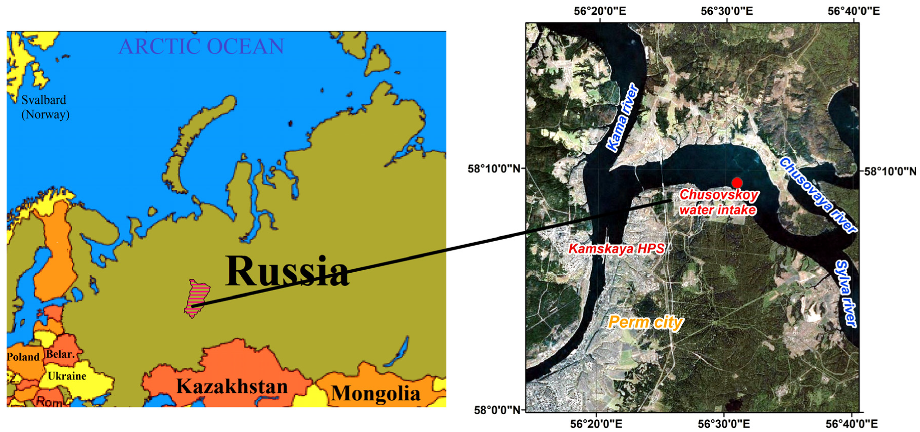
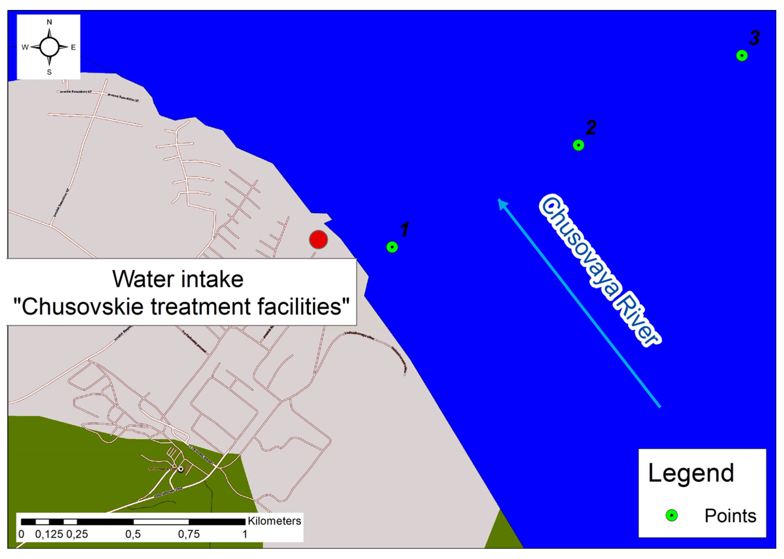
The study area is located immediately below the confluence of the Sylva and Chusovay rivers, in the zone of influence of the surge from the Kamskaya hydroelectric power station (Figure 1). The rivers under consideration have fairly close catchment areas: the river Chusovaya ~23 × 103 km2, and the river Sylva ~19.7 × 10³ km2. At the same time, the costs of spring flood and summer low water on the Chusovaya River are much more than on the Sylva River, at the same time, the costs of winter low water, due to the peculiarities of the catchment area of the Sylva River, are more than the costs of the Chusovaya River. A characteristic feature of rivers with deep winter low water, such as the river Sylva and Chusovaya, is the significantly lower variability in winter low water consumption compared to the runoff of spring flood. The nutrition of the studied rivers is mixed, with a predominance of snow. The share of snow-fed is about 55%, and of rainy—about 30%. About 18% is underground supply. The total mineralization of the waters of the Chusovaya River varies from 214 to 297 mg/L. The total hardness of the water is in the range of 2.3–3.5 mg-eq/L. Chusovaya River water belongs to hydrocarbonate-sulfate-calcium sodium hydrochemical facies. The total mineralization of the waters of the Sylva River varies from 680 to 760 mg/L. The total water hardness is in the range of 5.5–9.8 mg-eq/L. Sylva River water belongs to the sulfate-hydrocarbonate-calcium sodium hydrochemical facies.
Mineralization and, accordingly, water density of the Sylva River due to peculiarities of soil and geological structure of its basin determined by its high karsticity, is significantly higher than mineralization of the river Chusovaya. This leads to a very specific hydrochemical regime of the Chusovskoy reach. More saline, denser waters of the Sylva River “flow” under less dense waters of the Chusovaya River, while, in turn, waters of the river Chusovaya “overflow” waters of the river Sylva. Hydrological, hydrochemical, and hydrodynamic aspects of the confluence of these two watercourses were discussed in [17]. The main of them is that in winter the rivers of the considered region are replenished by groundwater. During the spring flood and summer low water, there are no significant differences in the quality of the waters of the Sylva and Chusovaya rivers. This is due to the predominance of rain feeding of rivers. Due to the geochemical features of the catchment area of the Sylva River basin, its waters during this period are characterized by significantly greater mineralization than the waters of the Chusovaya River. It was found that in the winter, downstream of the confluence of the Sylva and Chusovaya rivers, including the area of the Chusovskoy water intake of Perm, a rather stable two-layer structure of the water mass is generated. It means that the properties of water in the upper horizons are close to the properties of the water of the river Chusovaya, and in the lower horizons, they are close to the properties of water of the river Sylva. Another specific feature of the observed hydrological regime is the existence of a very distinct boundary between these water masses. In what follows, this boundary will be referred to as the “jump layer”. This boundary is characterized by a sharp change in the water density.
3. Materials and Methods
3.1. Field Research
In 2019, a series of field works was done in January and February 2019 to determine qualitative and quantitative characteristics of the Chusovskoy reach of the Kama reservoir near the Chusovsky water intake of Perm city. The density of the water is determined by both its temperature and mineralization. For winter conditions, the temperature distribution over the depth and width of the reservoir is almost uniform. Under these conditions, the general mineralization of water becomes a determining factor. Therefore, in conducting field studies, it is much more convenient to use a directly measured indicator—the conductivity of the water. The main advantages of this indicator are:
- -
- It is a very good linear connection with mineralization. As numerous studies have shown, these two indicators have a very stable relationship, the Pearson correlation coefficient is R2 ~0.96;
- -
- Specific electrical conductivity is very conveniently measured instrumentally using certified instruments. In our work, a professional device is used—the Cond 1970 conductormeter from WTW (Germany);
- -
- During measurements of specific electric conductivity, minimal disturbances are introduced into the water mass, which causes minimal metrologic distortions of the measured index.
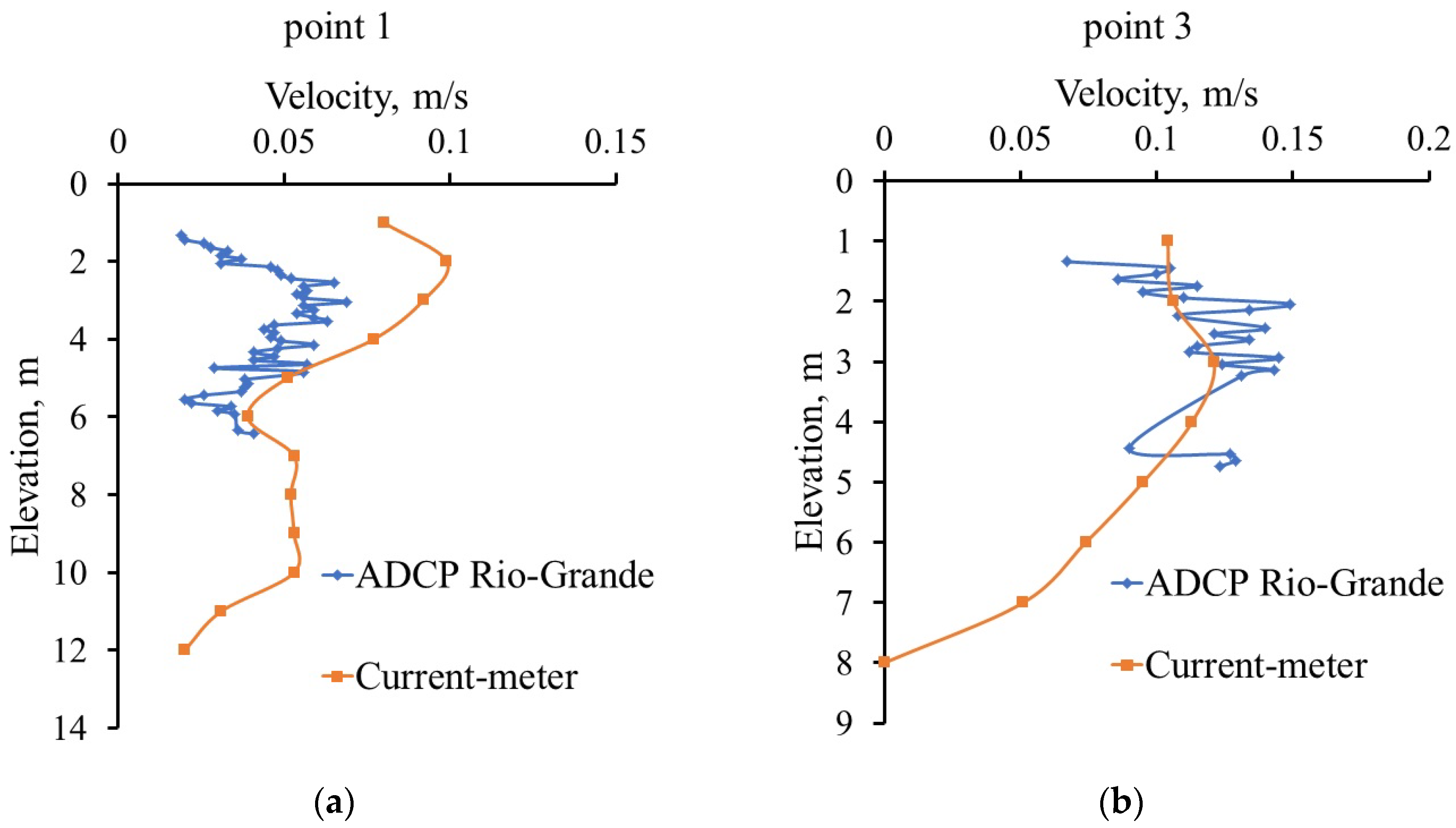
The study was performed using a Valeoport MIDAS ECM multiparameter flow meter and a WTW ProfLine 1970i portable conductometer. In addition to flow direction and velocity values, the Valeoport MIDAS ECM multi-parameter flowmeter allows one to measure water turbidity, conductivity, sound velocity in water, and temperature. The flow velocity range for this meter is from 0.001 m/s to 5 m/s. Flow velocities and directions were also measured by the GR-21 M hydrometric impeller and the Workhorse Rio Grande 600 acoustic Doppler current profiler (ADCP). The hydrometric impeller allows measurements of flow velocities in the range of 0.05–5 m/s, and in an acoustic profiler—in the range of 0.001 m/s to 5 m/s. The measurements were taken at the control verticals in the area near the water intake of the Chusovskie treatment facilities (CHTF), in the neighbor of the Talitsa settlement, and the Stary Lyady settlement.
The measurements were made at 3 verticals across the width of the section, at the prescribed horizons located at a depth of one or two meters from each other. Particular attention was paid to measurements in the area of the “jump layer”. Preliminary measurements were made using a WTW ProfLine 1970i portable conductivity meter, which allowed us to determine a depth-wise change in the reduced conductivity. The boundaries of the “jump layer” were determined based on these measurements. Then, the MIDAS ECM flow velocity meter was placed at the prescribed depth (upper boundary of “jump layer”, “jump layer”, below the “jump layer”) and started recording 30 s after the submersion to the preset depth. The duration of the recording is 10 min or more. Then the recording stops, and the devise is submerged deeper to the next horizon.
3.2. Numerical Model
A characteristic feature of the streams under consideration is their markedly different mineralization. Thus, in the Chusovaya River it is equal to ~380 mg/L, whereas in the Sylva River it can be ~950 mg/L depending on seasonal conditions. In the presence of such heterogeneity of impurity concentration in the confluent river waters, the formation of density currents demonstrates some peculiarities depending on the season. To study the formation of layered structures of confluent watercourses, numerical modeling was carried out within the framework of the three-dimensional approach. The calculations were performed based on the model for the description of turbulent flows. The problem was solved using the non-stationary approach.
The equation of motion is written in a tensor form as
where is density, are the components of velocity vector (), is the kinematic viscosity (m2/s). The turbulent viscosity is a function of the turbulent kinetic energy and its dissipation rate : [m2/s], where is a constant.
The equations for turbulent kinetic energy and its dissipation rate are written as
Here, is the generation of turbulent kinetic energy due to the mean velocity gradient, where is the norm of the mean strain rate tensor, ; is the generation of turbulent kinetic energy due to buoyancy, where is the gravity acceleration, is the turbulent Prandtl number, are the constants.
Since the acceleration vector of gravity is directed vertically downward and in the case of stable stratification the summand, describing the generation of turbulent kinetic energy due to buoyancy is negative , the turbulent kinetic energy decreases due to buoyancy.
The equation of impurity transport is written as
Here, is the diffusive flux of impurity determined by the expression , where is the molecular diffusion coefficient, is the effective turbulent diffusion coefficient, which depends on the turbulent viscosity : . The values of hydrodynamic constants were taken as follows [31]: ; ; ; ; ; ; .
The dependence of density on concentration was considered to be quadratic , ; in this case, the change in density throughout the depth was as high as 10%.
At the lower boundary of the computational domain, modelling the river bottom, the no-slip conditions and the absence of admixture flux were prescribed. The upper boundary of the domain, corresponding to the free surface of the liquid, was considered to be non-deformable and obey the condition for the absence of the normal velocity component and tangential stresses, as well as the condition for the absence of impurity flux. The lateral boundaries of the computational domain are assumed to fulfill the condition of zero normal derivative of the velocity and the absence of impurity flux:
At the inlet of the computational domain, the main flow velocity , which has one nonzero component, and the concentration equal to the background concentration of impurity in the river, were set as constant over the entire cross section:
At the outlet of the computational domain, the “soft” boundary conditions were prescribed: the vanishing of -coordinate derivatives of all field functions. The uniformly distributed background impurity concentration and the equality of the main flow velocity to the velocity at the inlet of the computational domain were used as the initial conditions:
Three-dimensional numerical simulation was performed using the ANSYS Fluent software package, which is based on the implementation of the finite volume method. To evaluate the effectiveness of the turbulence model, we performed test calculations using a higher-order model—the Reynolds stress model, in which seven additional equations for Reynolds stresses are solved. It was found that the difference in the results obtained by these models is not more than 5%. This turned to be good reason for using the model for further study. For the spatial discretization of the equations, a second-order scheme was used. The temporal evolution was modeled using an explicit second-order scheme.
4. Results
4.1. Field Measurement Results
The measurements made by the MIDAS ECM flow velocity meter are close to those made by the hydrometric impeller (Figure 2).
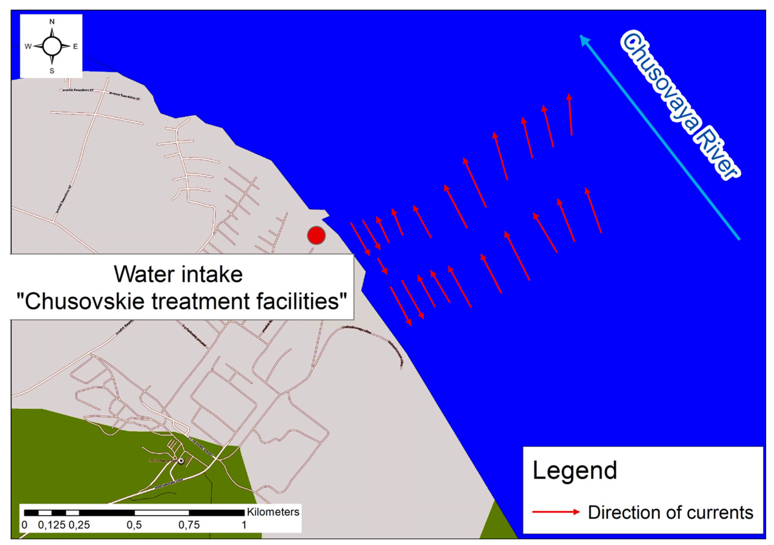
Here, it should be noted that the structure of flow fields in the water intake area is of a non-uniform character not only throughout the depth, but also over the water area. Maximum velocities (up to 0.1 m/s) are observed in the streambed part. In the streambed part and the right-bank part, the flow has the north and northwest direction, and in the left-bank part—the southeast direction (Figure 3). The “generator” of these increased flow velocities is a significant difference in salinity and, accordingly, in water density of the Sylva and Chusovaya rivers. Rather high flow velocities of up to 0.1–0.2 m/s are observed in the areas of the reservoirs with a high density heterogeneity of water masses (Figure 4). Figure 4 shows that the maximum water velocities are observed 2–3 m above the “jump layer”, the second maximum is observed 1–2 m below the jump layer.
The vertical heterogeneity of water masses was evaluated using the index of “specific electrical conductivity of water” measured in [mS/cm].
The main advantages of using this index are as follows:
- -
- Very good linear relationship of this index with mineralization;
- -
- Specific conductivity is very easy to measure instrumentally using certified devices. In particular, in this study a WTW professional conductivity meter ProfLine Cond 1970i (Germany) was used;
- -
- The process of conductivity measurements involves minimum perturbations of the water mass, and accordingly, minimum metrological distortions of the measured parameter.
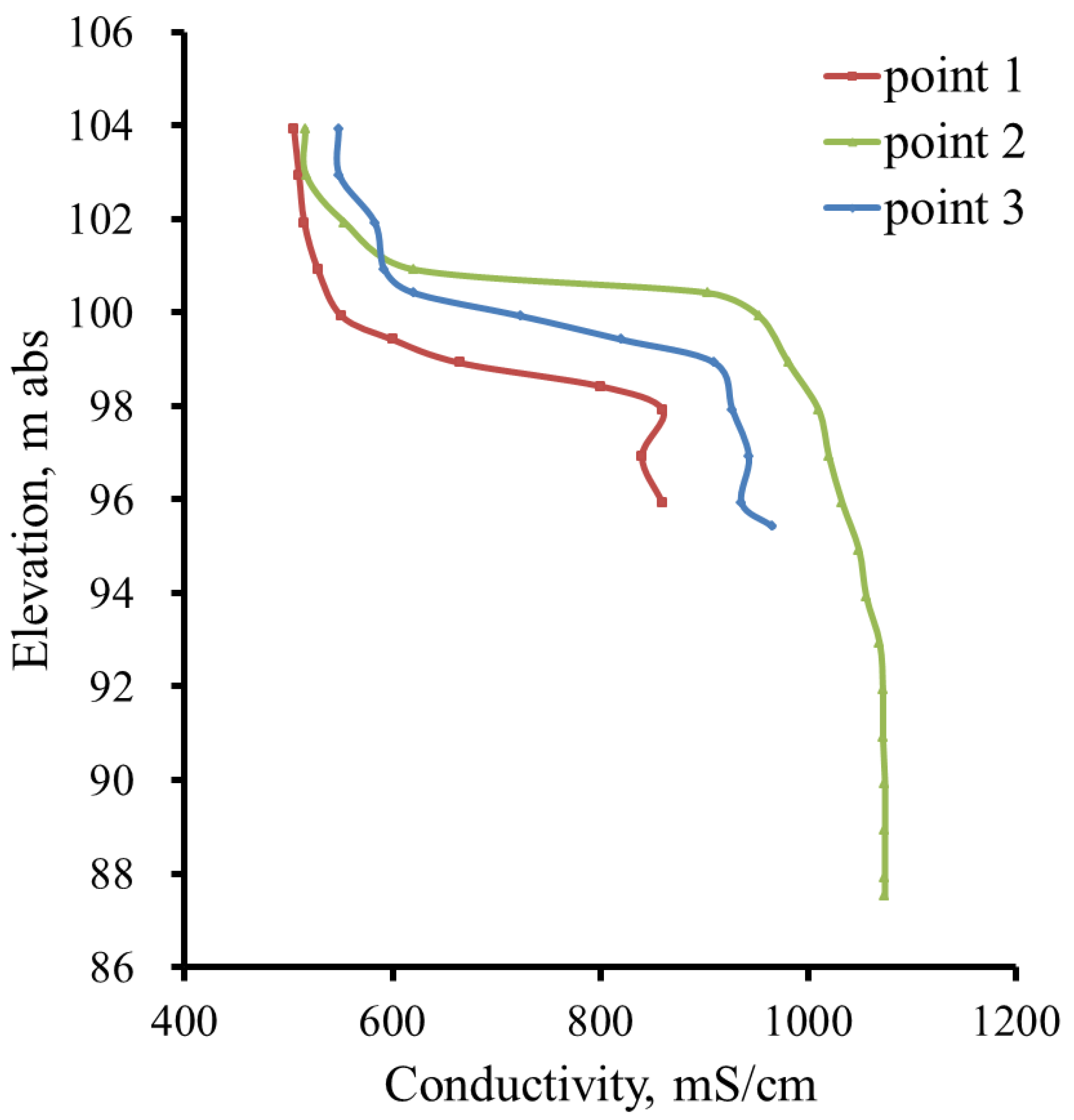
In the general case, the value of the specific conductivity of water is determined by the composition of dissolved ions, their concentration, and water temperature. The wide use of electrical conductivity index for the real-time control of water quality is primarily based on the linear relationship between the ion content and conductivity. Modern conductivity measuring devices can automatically correct for water temperature and reduce the measured values of æ to the relative temperature t = 250 °C. The closeness of the relationship between the total mineralization of water and the specific conductivity is determined by the stability of the chemical composition. In the area of water intake of the Chusovskie treatment facilities, the stable vertical heterogeneity determined by a qualitative difference in water compositions of the Sylva and Chusovaya rivers is generally formed in the winter season. The bottom layer contains mainly waters of the Sylva River, the salinity of which is 40–50% higher than the salinity of waters of the Chusovaya River. Figure 5 shows changes in the reduced specific conductivity at different verticals near the Chusovskoy water intake in March 2019.
Vertical 1 is located near the left bank, vertical 2—in the streambed part, and vertical 3—at a distance of 800 m from the right bank (Figure 6).
All three verticals show a similar pattern, the only difference being the elevation point for the boundaries of the “jump layer” of conductivity.
The in situ measurements made it possible to draw the following conclusions:
- -
- In the winter season, denser waters of the Sylva River flow under the less dense waters of the Chusovaya River;
- -
- Vertical stratification is observed not only downstream of the confluence of the two watercourses, but also in the areas of 15–20 km upstream of the confluence, i.e., waters of the Sylva River in the near-bottom area are distributed upstream of the Chusovaya River, and waters of the Chusovaya River in the near-surface layer are distributed upstream of the Sylva River;
- -
- Large-scale vortex structures are formed in this area of the Kama reservoir during the winter season. The energy of these structures is maintained due to a significant intraday irregularity of operation of the Kamskaya HPS and marked difference in the water density of the confluent Sylva and Chusovaya rivers.
A characteristic feature of the measured parameters in the examined zone is that they are subject to significant fluctuations, both seasonal and higher frequency fluctuations, which are associated with the presence of coherent structures. The seasonal variation in temperature and conductivity is shown in Figure 7. As evident from the Figure, in 2019 the maximum water hardness was observed during the winter season up to the middle of April reaching the value of 13 degrees.
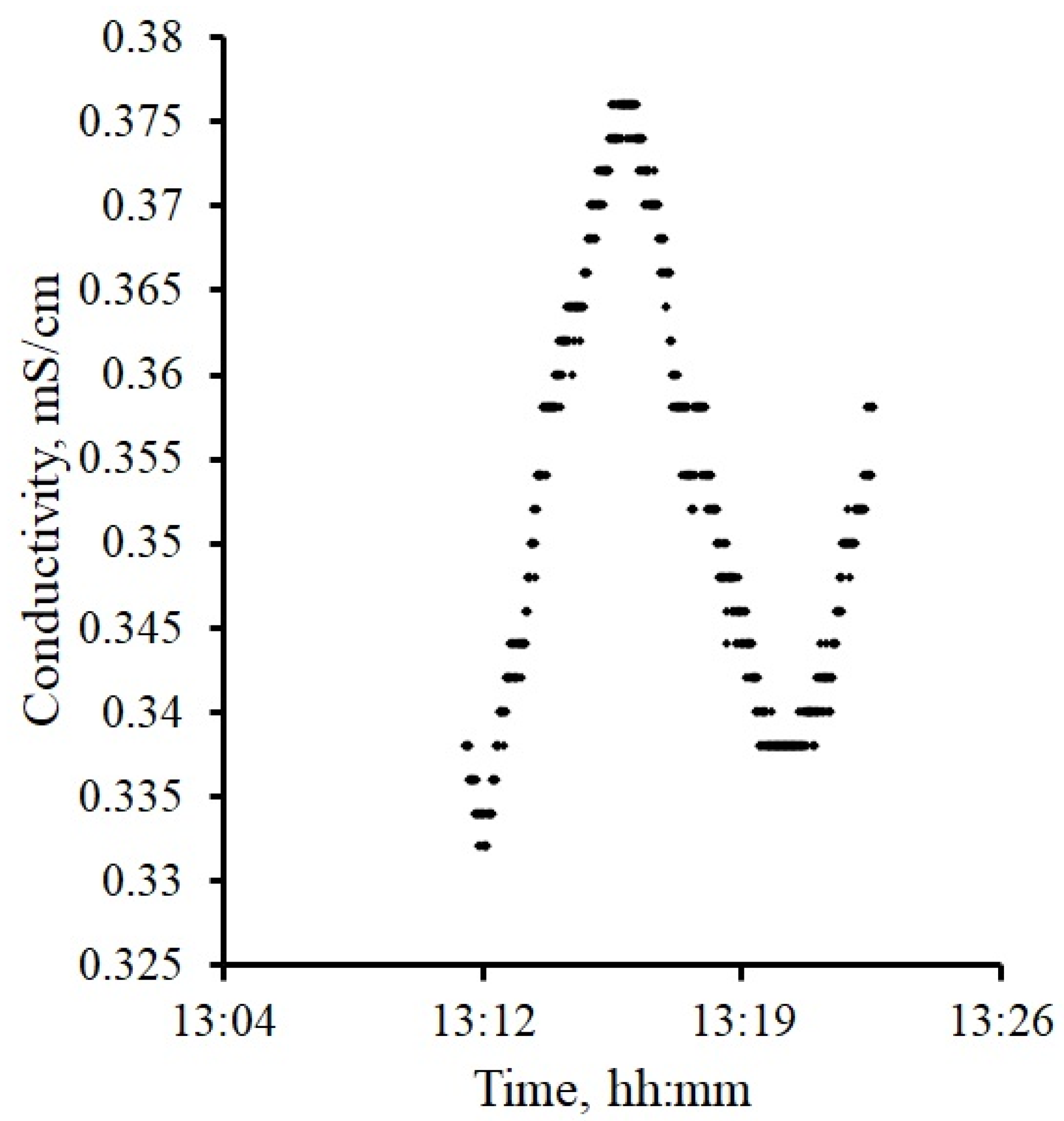
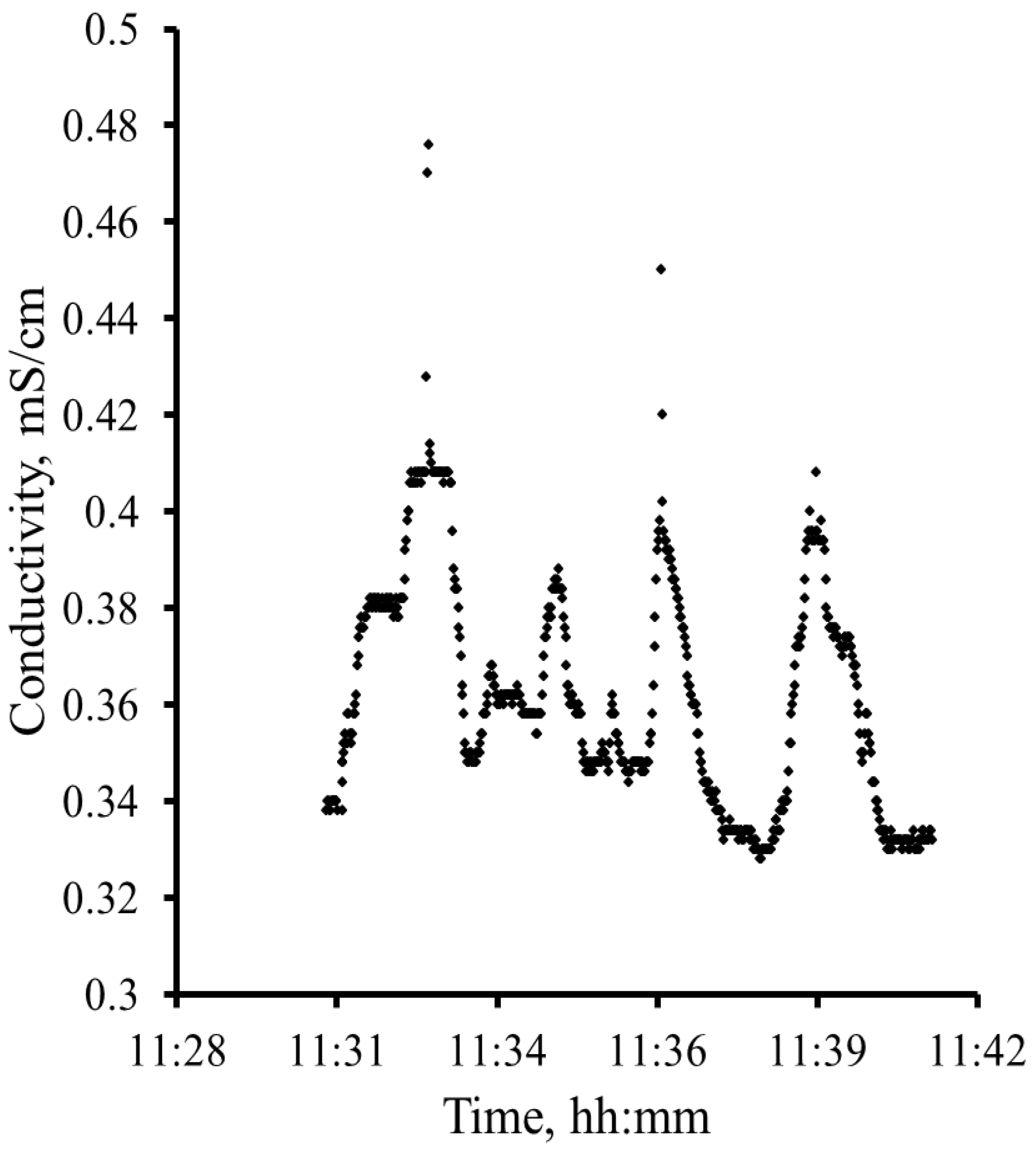
In addition to the well-known seasonal dynamics of water quality parameters, the long-term observations revealed significant, short periodic fluctuations of the examined parameters with periodicity T~2–10 min, which have not been previously detected and not described. In addition, in the area under consideration the measuring devices registered the wave-like fluctuations of the specific conductivity, whose amplitude in some cases were ~50% of the measured value (Figure 8 and Figure 9).
4.2. Numerical Results
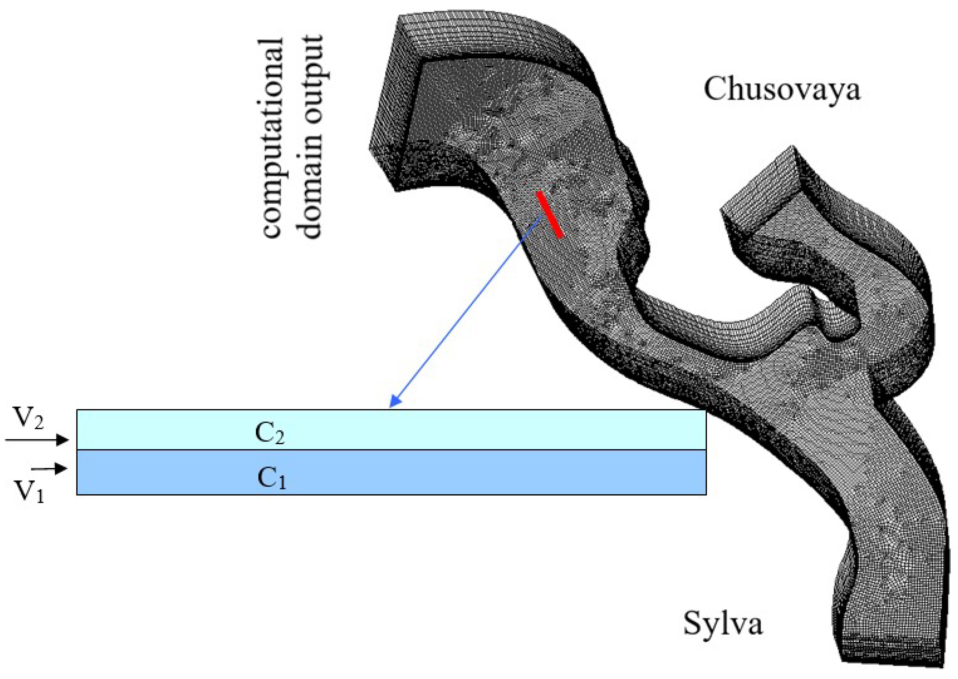
The calculations were performed for a 300-meter-long stretch of the Chusovaya River downstream of the confluence of the Chusovaya and Sylva rivers. This section is located in the streambed section in the area of water intake. A regime established in this section over the winter–spring period is characterized by the presence of a steady layer of density and velocity jumps. Previous in situ measurements have revealed temporal fluctuations of water hardness. To simulate the observed phenomenon, we solved the problem of interaction between two flows of liquids with different densities. The computational scheme is shown in Figure 10. The depth of the investigated area was taken as a constant, and equal to 20 m.
The computational grid was built using the software package entering into ANSYS Fluent. The number of nodes throughout the depth of the computational domain was taken equal to 100, and the grid was uniform. Horizontally, the grid consisted of quadrilateral cells uniformly distributed along the entire length, with a characteristic linear size of 0.2 m.
Calculations were performed for different flow rates of water through the Chusovaya and Sylva rivers. The values of parameters for different variants of computation are given in Table 1. The relative difference in flow velocities is determined by the formula: Pv = V1/V2. In all variants of calculations, the concentration distribution at the initial time is given as a delta function of the depth. At a depth of 10 m, the concentration of salt in the water is 950 mg/L, whereas at a depth of more than 10 m, the concentration of salt in the water is 380 g/L.
As time goes, the field of impurity concentration changes, but due to a very low diffusion rate, the boundary is still clearly defined. Visualization of the full-scale blurring of concentration is rather weak (Figure 11). Such pattern persists in all variants of calculations.
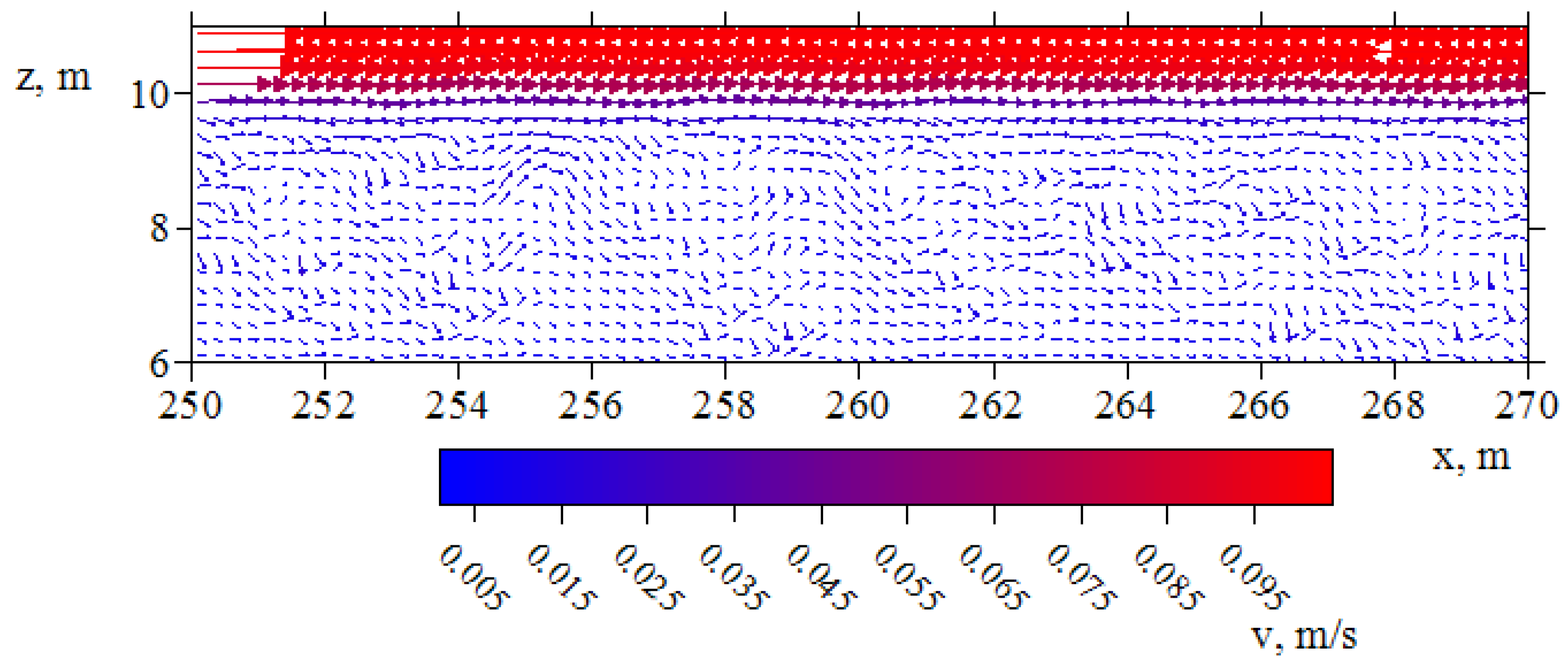
In the course of time, the formation of vortex structures is observed near the jump layer (Figure 12). This leads to temporal fluctuations of concentration at a point in space and to a wave structure of the instantaneous concentration field (Figure 13). Figure 12, Figure 13 and Figure 14 show the results of simulation made for the first set of parameters.
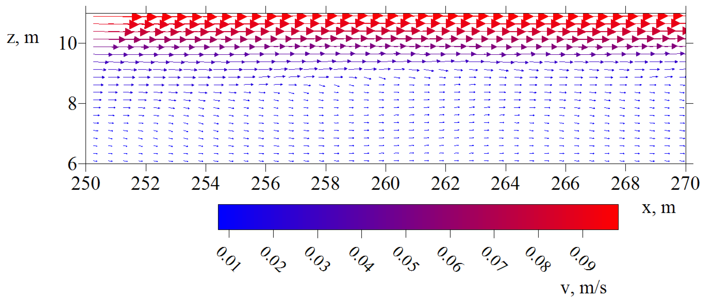
Temporal fluctuations of concentration at a point are shown in Figure 14. Since these fluctuations are localized in and near the jump layer, the Figure 12 and Figure 13 show the velocity vector field and the concentration field in a twenty-meter section of the computational domain within the interval from 250 m to 270 m. The velocity vector field (Figure 12) demonstrates the existence of irregular vortex structures. These structures are responsible for the formation of waves in the concentration field (Figure 13).
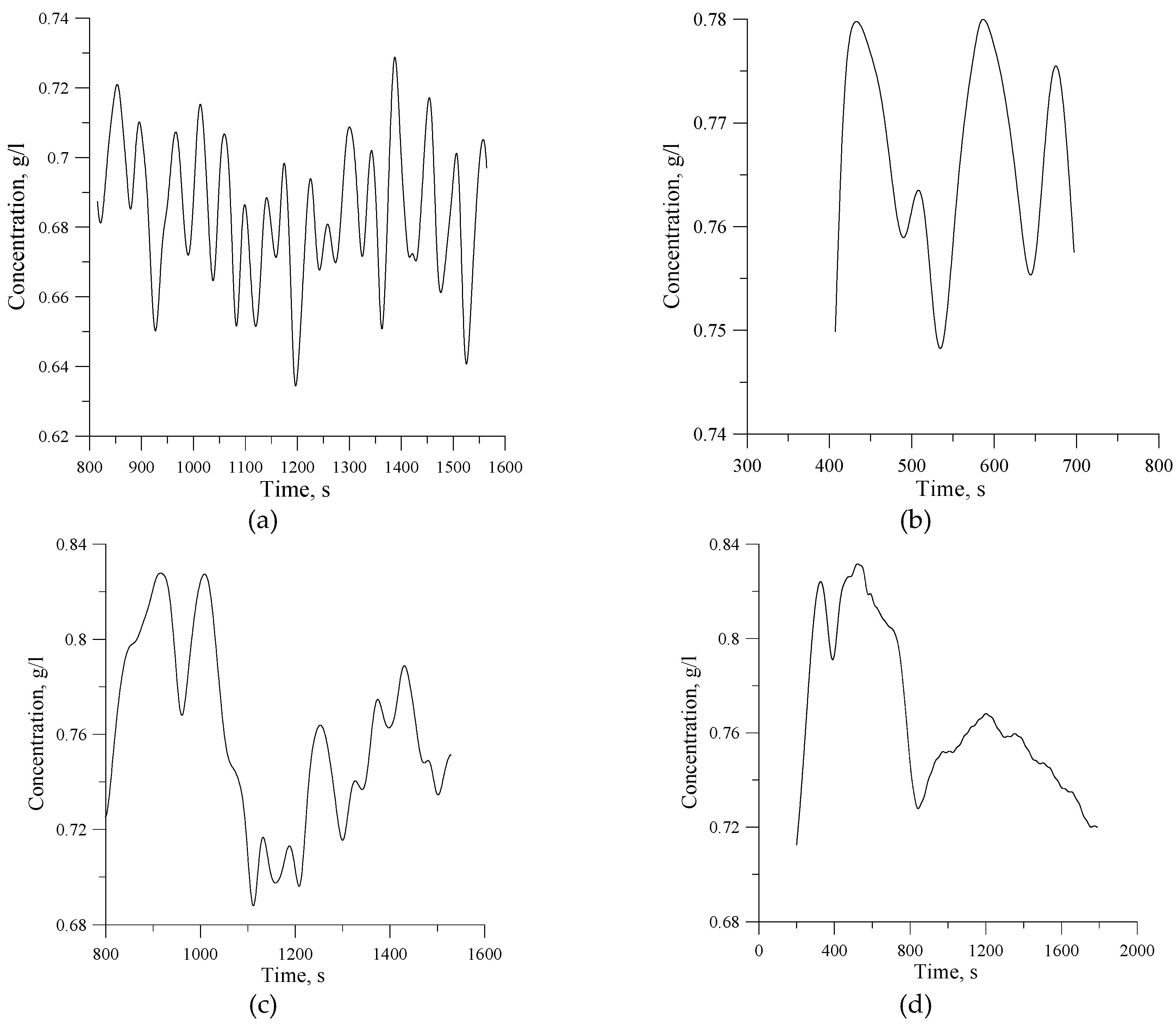
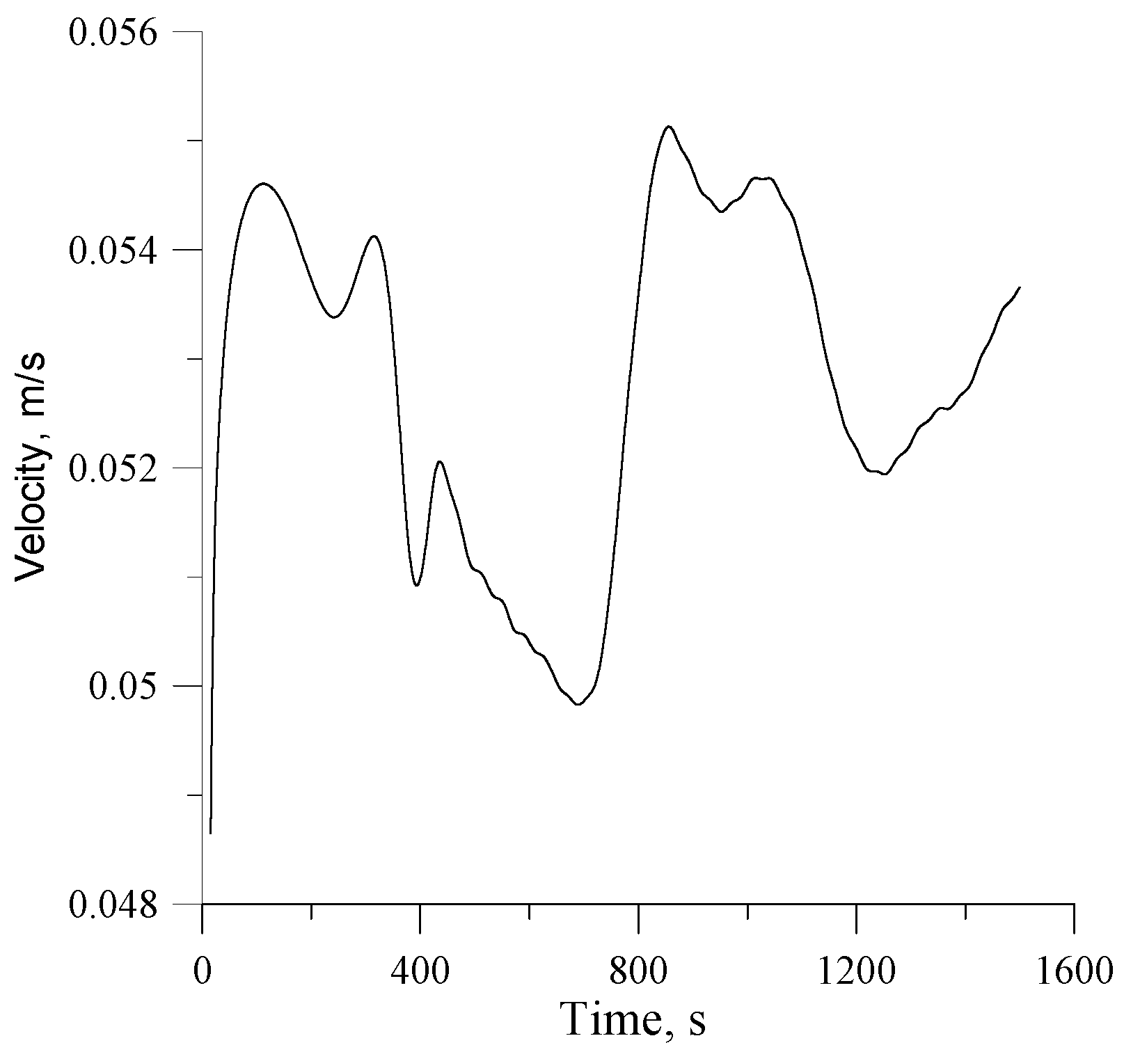
The temporal evolutions of concentration at a point is shown in Figure 14. The observable temporal regularity of fluctuations with a period of about a minute was found experimentally during in situ measurements (Figure 14a). Variants of calculations differ from each other by the ratio of flow velocities in water masses of different concentrations. As the ratio of flow rates in the water of different concentrations decreases, the period of vortex structure oscillations increases (Figure 14b,c). For the velocity ratio Pv = 0.5 (Figure 14d and Figure 15), the period of oscillations is slightly longer than 20 min, while the scale of vortex structures increases, and the wave number decreases. The intensity of such structures is much less than for Pv = 10, at which the period is about one minute. It means that with increase of the velocities ratio by 20 times, the period of oscillations decreases practically by the same factor.
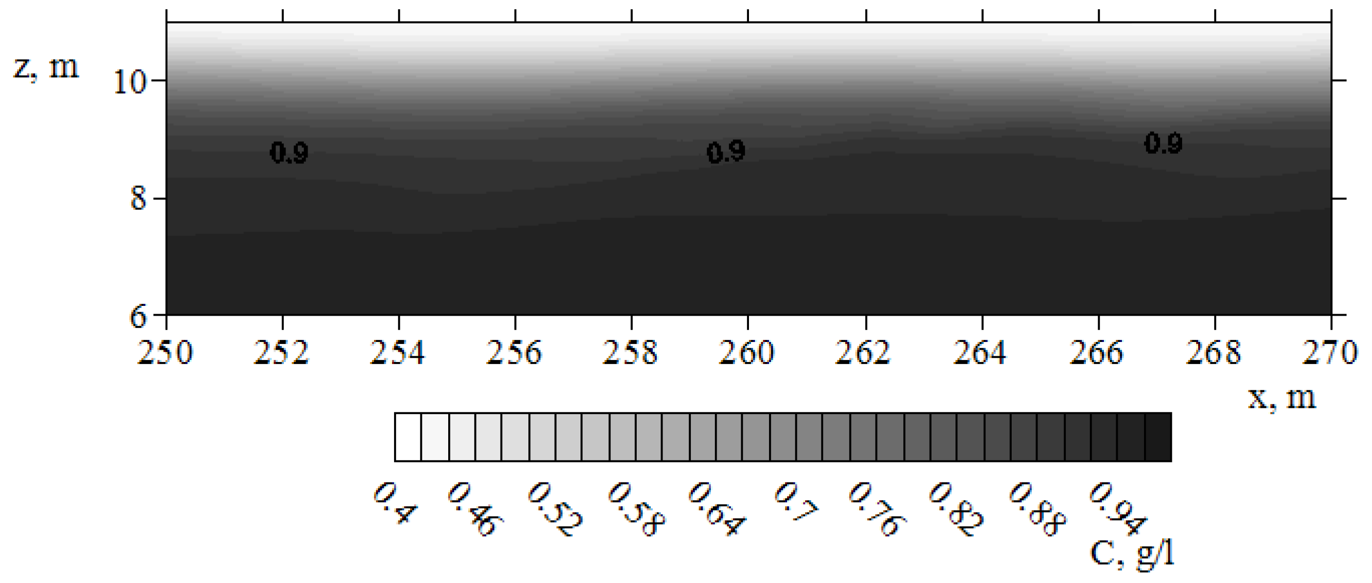
Figure 16 and Figure 17 show the concentration field and velocity vector field in the section of the computational domain corresponding to the sections in Figure 14a,b, 250 to 270 m in length. As can be seen from Figure 16, the wave pattern of concentration distribution in the jump layer is maintained. However, with decreasing velocity ratio of flows with different concentrations, the spatial scale increases and oscillations are characterized by a smaller wave number. As is evident from the vector pattern of the velocity field (Figure 17), the vortex structure is of second order and only the main fluid flow can be visualized.
5. Discussion
The sustainability of public and industrial water supply is one of the most important indicators of the viability and success of the industrial sector. This problem is especially acute for territories located in river confluence zones with different water composition characteristics. Water intake devices created in these areas for the purposes of drinking and service water supply must have a number of features that must be laid down during their design and operation. In winter, during the transition to underground feeding, the mineralization of the water of the river. Sylva, due to the significant karsting of its basin, significantly, 2–3 times, increases in comparison with the mineralization of the water of the river Chusovoy. Accordingly, the densities of the merging water masses also change. Under conditions of backwater from the Kamskaya HPP located below, the flow velocities are very low, respectively, the density Froude number, which characterizes the stability of stratified water masses, becomes less than the critical value and stable stratification is observed (where Δρ/ρ is the relative difference in the densities of water masses). The hydrodynamic aspects of this layered structure are described in detail in [17].
Previous studies [26,32] have shown that large-scale coherent structures forming inside and near the water mixing region play an important role in improving mixing and pulse exchange between the two streams. A shallow mixing layer containing mainly co-rotating vortices is formed due to Kelvin–Helmholtz instability [33]. The average size of these vortices increases from the confluence due to the fusion of the vortices until the effects of friction against the bottom become large enough to mate the vortices. In case of density difference there is effect of more dense layers flowing under liquid layers of lower density, at that large-scale vortex is formed in horizontal direction with dimensions three orders of magnitude exceeding characteristic vertical scale [17]. Within the scope of the present work, it has been shown that within the large-scale vertical structures found in [17] small-scale vortex structures are observed, the characteristics of which depend on the rate of merging flows.
Currently, the issues of analysis of coherent structures of water masses forming at the boundaries of partitions are becoming more and more relevant. This is connected not only with the hydrodynamic formation of stable layered structures in surface water bodies, but with the tasks of practical use of these effects in the tasks of water protection and ensuring sustainable water use. Articles [34,35] examine interfaces in density flows. The paper [36] examines large-scale coherent structures formed in free Rayleigh–Benard-type convective flows in large lakes. Work [37] considers the formation of coherent structures associated with the impact of wind loads on the water surface. The materials of works [38,39] discusses the issues of observation and analysis of large-scale coherent structures formed in gravitational flows. Publication [40] presents the results of three-dimensional direct numerical modeling of gravitational currents at different values of Reynolds and Schmidt numbers. Significant effects of Schmidt number on density distribution and interface stability are shown. Three-dimensional RANS modeling of unsteady discontinuous gravitational currents is considered in [41].
Thus, the main practical result of the completed complex of studies is that when organizing the selective extraction of water from a water body characterized by significant vertical stratification of water masses, it is necessary to take into account possible coherent structures arising at the interface of water masses. These structures can make it very difficult to organize selective water intake. This problem arises primarily in the organization of selective water intake using bottom barriers. The choice of the optimal height of the bottom barrier cutting off the water intake from the bottom layers is a very important task [26]. As a rule, its mouth is poured at the height of the location of the density jump layer. However, as the studies have shown, it is also necessary to take into account the intensity of coherent structures arising at the interface of water masses [30]. At the same time, the scale of these structures is determined by the ratio of both mineralizations, densities of water masses and flow rates.
6. Conclusions
In this study, we investigated the character of wave structure formation in the winter season in the zone of confluence of the Sylva and Chusovaya rivers near Chusovskoy water intake. It was found that downstream of the confluence, due to a significant difference in mineralization of waters of the Sylva and Chusovaya rivers, a water layer with maximum density and, accordingly, maximum mineralization and hardness is formed in the near-bottom area. According to in situ measurements made during the winter low-water period in the area of the Chusovskoy water intake located 8 km downstream of the confluence, there are significant fluctuations in the concentration and flow velocity in the density jump layer. Numerical simulation in the 3D formulation allowed us to reproduce vortex structures formed in the jump layer and estimate their parameters. It was shown that these vortex structures lead to concentration fluctuations in space and time. The period and spatial scale of these vortex structures are determined by the ratio of flow velocities and differences in the salinities and, respectively, in densities of the water masses being considered. The period of oscillations is directly proportional to the ratio of flow velocities, all other parameters being stable.
These assessments are of fundamental importance for implementation of stable selective intake of water with the required consumer properties.
Author Contributions
Conceptualization, T.P.L. and A.P.L.; methodology, T.P.L. and A.P.L.; validation, T.P.L., A.P.L. and Y.N.P.; investigation, Y.N.P. and A.V.B.; writing—original draft preparation, T.P.L., A.P.L. and Y.N.P.; writing—review and editing, T.P.L., A.P.L. and Y.N.P. All authors have read and agreed to the published version of the manuscript.
Funding
Data Availability Statement
The data supporting reported results are available from the corresponding author on reasonable request.
Conflicts of Interest
The authors declare no conflict of interest.
References
- Macdonald, D.D.; Ingersoll, C.G.; Berger, T.A. Development and Evaluation of Consensus-Based Sediment Quality Guidelines for Freshwater Systems. Arch. Environ. Contam. Toxicol. 2000, 39, 20–31. [Google Scholar] [CrossRef] [PubMed]
- Ucler, N.; Engin, G.O.; Kocken, H.G.; Öncel, M.S. Game theory and fuzzy programming approaches for bi-objective optimization of reservoir watershed management: A case study in Namazgah reservoir. Environ. Sci. Pollut. Res. 2015, 22, 6546–6558. [Google Scholar] [CrossRef] [PubMed]
- Lopes, L.F.G.; Carmo, J.S.D.; Cortes, R.M.V.; Oliveira, D. Hydrodynamics and water quality modelling in a regulated river segment: Application on the instream flow definition. Ecol. Model. 2004, 173, 197–218. [Google Scholar] [CrossRef]
- Na, E.H.; Park, S.S. A hydrodynamic and water quality modeling study of spatial and temporal patterns of phytoplankton growth in a stratified lake with buoyant incoming flow. Ecol. Model. 2006, 199, 298–314. [Google Scholar] [CrossRef]
- Chen, Q.; Tan, K.; Zhu, C.; Li, R. Development and application of a two-dimensional water quality model for the Daqinghe River Mouth of the Dianchi Lake. J. Environ. Sci. 2009, 21, 313–318. [Google Scholar] [CrossRef]
- Calderon, M.R.; Almeida, C.A.; González, P.; Jofré, M.B. Influence of water quality and habitat conditions on amphibian community metrics in rivers affected by urban activity. Urban Ecosyst. 2019, 22, 743–755. [Google Scholar] [CrossRef]
- Zhao, L.; Zhang, X.; Liu, Y.; He, B.; Zhu, X.; Zou, R.; Zhu, Y. Three-dimensional hydrodynamic and water quality model for TMDL development of Lake Fuxian, China. J. Environ. Sci. 2012, 24, 1355–1363. [Google Scholar] [CrossRef]
- Liu, W.C.; Liu, S.Y.; Hsu, M.H.; Kuo, A.Y. Water quality modeling to determine minimum instream flow for fish survival in tidal rivers. J. Environ. Manag. 2005, 76, 293–308. [Google Scholar] [CrossRef]
- Bai, J.; Xiao, R.; Zhang, K.; Gao, H. Arsenic and heavy metal pollution in wetland soils from tidal freshwater and salt marshes before and after the flow-sediment regulation regime in the Yellow River Delta, China. J. Hydrol. 2012, 450, 244–253. [Google Scholar] [CrossRef]
- Endo, I.; Walton, M.; Chae, S.; Park, G.-S. Estimating Benefits of Improving Water Quality in the Largest Remaining Tidal Flat in South Korea. Wetlands 2012, 32, 487–496. [Google Scholar] [CrossRef]
- Wu, Y.; Chen, J. Estimating irrigation water demand using an improved method and optimizing reservoir operation for water supply and hydropower generation: A case study of the Xinfengjiang reservoir in southern China. Agric. Water Manag. 2013, 116, 110–121. [Google Scholar] [CrossRef]
- Wu, Y.; Chen, J. Investigating the effects of point source and nonpoint source pollution on the water quality of the East River (Dongjiang) in South China. Ecol. Indic. 2013, 32, 294–304. [Google Scholar] [CrossRef]
- Jiang, T.; Zhong, M.; Cao, Y.; Zou, L.; Lin, B.; Zhu, A. Simulation of water quality under different reservoir regulation scenarios in the tidal river. Water Res. Manag. 2016, 30, 3593–3607. [Google Scholar] [CrossRef]
- Rahman, S.; Hossain, F. Spatial assessment of water quality in peripheral rivers of Dhaka city for optimal relocation of water intake point. Water Res. Manag. 2008, 22, 377–391. [Google Scholar] [CrossRef]
- Biswas, T.; Mosley, L. From mountain ranges to sweeping plains, in droughts and flooding rains; river Murray water quality over the last four decades. Water Res. Manag. 2019, 33, 1087–1101. [Google Scholar] [CrossRef]
- Li, K.; Zhu, C.; Wu, L.; Huang, L. Problems caused by the Three Gorges Dam construction in the Yangtze River basin: A review. Environ. Rev. 2013, 21, 127–135. [Google Scholar] [CrossRef]
- Lyubimova, T.; Lepikhin, A.; Parshakova, Y.; Konovalov, V.; Tiunov, A. Formation of the density currents in the zone of confluence of two rivers. J. Hydrol. 2014, 508, 328–342. [Google Scholar] [CrossRef]
- Lyubimova, T.; Lepikhin, A.; Parshakova, Y.; Tiunov, A. The risk of river pollution due to washout from contaminated floodplain water bodies in periods of high magnitude floods. J. Hydrol. 2016, 534, 579–589. [Google Scholar] [CrossRef]
- Lyubimova, T.; Parshakova, Y.; Lepikhin, A.; Lyakhin, Y.; Tiunov, A. Application of hydrodynamic modeling in 2D and 3D approaches for the improvement of the recycled water supply systems of large energy complexes based on reservoirs-coolers. Int. J. Heat Mass Transfer. 2019, 140, 897–908. [Google Scholar] [CrossRef]
- Jiang, C.; ·Constantinescu, G.; Yuan, S.; Tang, H. Flow hydrodynamics, density contrast effects and mixing at the confluence between the Yangtze River and the Poyang Lake channel. Environ. Fluid Mech. 2022, 107, 1–29. [Google Scholar] [CrossRef]
- Cheng, Z.; Constantinescu, G. Stratification effects on hydrodynamics and mixing at a river confluence with discordant bed. Environ. Fluid Mech. 2020, 4, 843–872. [Google Scholar] [CrossRef]
- Constantinescu, G.; Miyawaki, S.; Rhoads, B.; Sukhodolov, A.; Kirkil, G. Structure of turbulent flow at a river confluence with a momentum and velocity ratios close to 1: Insight from an eddy-resolving numerical simulation. Water Resour. Res. 2011, 47, W05507. [Google Scholar] [CrossRef]
- Gualtieri, C.; Filizola, N.; de Oliveira, M.; Martinelli Santos, A.; Ianniruberto, M. A field study of the confluence between egro and Solimes Rivers Part 1: Hydrodynamics and sediment transport. Comptes Rendus Geosci. 2018, 350, 31–42. [Google Scholar] [CrossRef]
- Ianniruberto, M.; Trevethan, M.; Pinheiro, A.; Andrade, J.F.; Dantas, E.; Filizola, N.; Gualtieri, C. A field study of the confluence between Negro and Solimes Rivers. Part 2: Bed morphology and stratigraphy. Comptes Rendus Geosci. 2018, 350, 43–54. [Google Scholar] [CrossRef]
- Ramón, C.L.; Armengol, J.; Dolz, J.; Prats, J.; Rueda, F. Mixing dynamics at the confluence of two large rivers undergoing weak density variations. J. Geophys. Res. Ocean. 2014, 119, 2386–2402. [Google Scholar] [CrossRef]
- Rhoads, B.; Sukhodolov, A. Spatial and temporal structure of shear layer turbulence at a river confluence. Water Resour. Res. 2004, 40, W06304. [Google Scholar] [CrossRef]
- Sukhodolov, A.N.; Sukhodolova, T.A. Dynamics of fow at concordant gravel bed river confluences: Effects of junction angle and momentum flux ratio. J. Geophys. Res. Earth Surf. 2019, 124, 588–615. [Google Scholar] [CrossRef]
- Lyubimova, T.; Parshakova, Y.; Lepikhin, A.; Lyakhin, Y.; Tiunov, A. The effect of unsteady water discharge through dams of hydroelectric power plants on hydrodynamic regimes of the upper pools of waterworks. Water 2020, 12, 1336. [Google Scholar] [CrossRef]
- Lyubimova, T.; Lepikhin, A.; Parshakova, Y.; Bogomolov, A.; Lyakhin, Y. The Influence of Intra-Day Non-Uniformity of Operation of Large Hydroelectric Power Plants on the Performance Stability of Water Intakes Located in Their Upper Pools. Water 2021, 13, 3577. [Google Scholar] [CrossRef]
- Lyubimova, T.; Lepikhin, A.; Parshakova, Y.; Bogomolov, A.; Lyakhin, Y.; Tiunov, A. Peculiarities of hydrodynamics of small surface water bodies in zones of active technogenesis (on the example of the Verkhne-Zyryansk reservoir, Russia). Water 2021, 13, 1638. [Google Scholar] [CrossRef]
- Launder, B.; Spalding, D. Lectures in Mathematical Models of Turbulence; Academic Press: London, UK, 1972; 169p. [Google Scholar]
- Constantinescu, G. LE of shallow mixing interfaces: A review. Environ. Fluid Mech. 2014, 14, 971–996. [Google Scholar] [CrossRef]
- Cheng, Z.; Constantinescu, G. Near-field and far-field structure of shallow mixing layers. J. Fluid Mech. 2020, 904, A21. [Google Scholar] [CrossRef]
- Neamtu-Halic, M.; Krug, D.; Haller, G.; Holzner, M. Lagrangian coherent structures and entrainment near the turbulent/non-turbulent interface of a gravity current. J. Fluid Mech. 2019, 877, 824–843. [Google Scholar] [CrossRef] [Green Version]
- Krug, D.; Holzner, M.; Lüthi, B.; Wolf, M.; Kinzelbach, W.; Tsinober, A. The turbulent/non-turbulent interface in an inclined dense gravity current. J. Fluid Mech. 2015, 765, 303–324. [Google Scholar] [CrossRef] [Green Version]
- Smirnov, S.; Smirnovsky, A.; Bogdanov, S. The Emergence and Identification of Large-Scale Coherent Structures in Free Convective Flows of the Rayleigh-Bénard Type. Fluids 2021, 6, 431. [Google Scholar] [CrossRef]
- Sanjou, M.; Nezu, I.; Toda, A. Coherent turbulence structure generated by wind-induced water waves. In Proceedings of the International Conference on Fluvial Hydraulics—Riverflow, Braunschweig, Germany, 8–10 September 2010; pp. 1673–1680. [Google Scholar]
- Marshall, C.R.; Dorrell, R.M.; Keevil, G.M.; Peakall, J.; Tobias, S.M. Observations of large-scale coherent structures in gravity currents: Implications for flow dynamics. Exp. Fluids 2021, 62, 1–18. [Google Scholar] [CrossRef]
- Balasubramanian, S.; Zhong, Q. Entrainment and mixing in lock-exchange gravity currents using simultaneous velocity-density measurements. Phys. Fluids 2018, 30, 056601. [Google Scholar] [CrossRef] [Green Version]
- Marshall, R.; Dorrell, M.; Dutta, S.; Keevil, M.; Peakall, J.; Tobias, M. The effect of Schmidt number on gravity current flows: The formation of large-scale three-dimensional structures. Phys. Fluids 2021, 33, 106601. [Google Scholar] [CrossRef]
- Paik, J.; Eghbalzadeh, A.; Sotiropoulos, F. Three-Dimensional Unsteady RANS Modeling of Discontinuous Gravity Currents in Rectangular Domains. J. Hydraul. Eng. 2009, 135, 505–521. [Google Scholar] [CrossRef]
Figure 1.
Location of the monitored area.

Figure 2.
Comparison of flow velocity changes measured by the Rio Grande and GR-21M measuring devices: (a) - for measurements at point 1; (b) - for measurements at point 3.
Figure 2.
Comparison of flow velocity changes measured by the Rio Grande and GR-21M measuring devices: (a) - for measurements at point 1; (b) - for measurements at point 3.

Figure 3.
Direction of flows in the area of the water intake facility of the Chusovskie treatment facilities in the city of Perm.
Figure 3.
Direction of flows in the area of the water intake facility of the Chusovskie treatment facilities in the city of Perm.

Figure 4.
Depth-wise variation of flow velocities in the area of Chusovskoy water intake complex.

Figure 5.
Changes in the reduced specific conductivity in the water intake area of the Chusovskie treatment facilities.
Figure 5.
Changes in the reduced specific conductivity in the water intake area of the Chusovskie treatment facilities.

Figure 6.
Location of verticals, at which the reduced specific conductivity is measured.

Figure 7.
Changes in water hardness and temperature values in 2019 (from January to September) in the area of water intake structure of the Chusovskie treatment facilities (CHTF).
Figure 7.
Changes in water hardness and temperature values in 2019 (from January to September) in the area of water intake structure of the Chusovskie treatment facilities (CHTF).

Figure 8.
Fluctuations of specific conductivity of water at a depth of 1 m.

Figure 9.
Fluctuations of specific conductivity of water at a depth of 2.5 m.

Figure 10.
The red line marks the region, for which a series of computations were conducted to model the occurrence of waves in the density jump layer. The length of the computational domain is 300 m.
Figure 10.
The red line marks the region, for which a series of computations were conducted to model the occurrence of waves in the density jump layer. The length of the computational domain is 300 m.

Figure 11.
Concentration field after 2 h of computation.

Figure 12.
Concentration field after 2 h of computation. Pv = 10.

Figure 13.
Concentration field near the jump layer. The concentration is shown in g/L. Pv = 10.

Figure 14.
Changes in impurity concentration at a depth of 10 m for the computational domain of 20 m in depth, (a) Pv = 10, (b) Pv = 5, (c) Py = 2, (d) Py = 0.5.
Figure 14.
Changes in impurity concentration at a depth of 10 m for the computational domain of 20 m in depth, (a) Pv = 10, (b) Pv = 5, (c) Py = 2, (d) Py = 0.5.

Figure 15.
Variation of velocity modulus at a depth of 10 m for a computational domain of 20 m in depth, Pv = 0.5.
Figure 15.
Variation of velocity modulus at a depth of 10 m for a computational domain of 20 m in depth, Pv = 0.5.

Figure 16.
Concentration field near the jump layer. Concentrations are given in g/L. Pv = 0.5.

Figure 17.
Velocity vector field near the jump layer. Values are given in m/s. Pv = 0.5.


Table 1.
Parameters of computational experiment variants.
| № of Variant | Flow Rates | Relative Difference in the Velocities of Flows with Different Concentrations | Impurity Concentration, mg/L | Depth of Jump Layer Location, m |
|---|---|---|---|---|
| 1 | V1 = 0.01 + 0.001 × ln(z/e) m/s, V2 = 0.1 m/s | Pv = 10 | C1 = 380, C2 = 950 | 10 |
| 2 | V1 = 0.01 + 0.001 × ln(z/e) m/s, V2 = 0.05 m/s | Pv = 5 | C1 = 380, C2 = 950 | 10 |
| 3 | V1 = 0.01 + 0.001 × ln(z/e) m/s, V2 = 0.02 m/s | Pv = 2 | C1 = 380, C2 = 950 | 10 |
| 4 | V1 = 0.05 + 0.005 × ln(z/e) m/s, V2 = 0.1 m/s | Pv = 0.5 | C1 = 380, C2 = 950 | 10 |
Publisher’s Note: MDPI stays neutral with regard to jurisdictional claims in published maps and institutional affiliations. |
© 2022 by the authors. Licensee MDPI, Basel, Switzerland. This article is an open access article distributed under the terms and conditions of the Creative Commons Attribution (CC BY) license (https://creativecommons.org/licenses/by/4.0/).
Share and Cite
MDPI and ACS Style
Lyubimova, T.P.; Lepikhin, A.P.; Parshakova, Y.N.; Bogomolov, A.V. Coherent Structures at the Interface between Water Masses of Confluent Rivers. Water 2022, 14, 1308. https://doi.org/10.3390/w14081308
AMA Style
Lyubimova TP, Lepikhin AP, Parshakova YN, Bogomolov AV. Coherent Structures at the Interface between Water Masses of Confluent Rivers. Water. 2022; 14(8):1308. https://doi.org/10.3390/w14081308
Chicago/Turabian StyleLyubimova, T. P., A. P. Lepikhin, Ya N. Parshakova, and A. V. Bogomolov. 2022. "Coherent Structures at the Interface between Water Masses of Confluent Rivers" Water 14, no. 8: 1308. https://doi.org/10.3390/w14081308
Note that from the first issue of 2016, this journal uses article numbers instead of page numbers. See further details here.