
Semi-Analytical Model for the Evaluation of Shoreline Recession Due to Waves and Sea Level Rise


Department of Construction, Civil Engineering and Architecture (DICEA), Università Politecnica delle Marche, 60131 Ancona, Italy
*
Author to whom correspondence should be addressed.
Water 2022, 14(8), 1305; https://doi.org/10.3390/w14081305
Submission received: 7 April 2022
/
Revised: 13 April 2022
/
Accepted: 15 April 2022
/
Published: 17 April 2022
(This article belongs to the Special Issue Ocean Wave Studies for Engineering Applications)
Abstract
:The climate change process is leading to an increase in the sea level and the storm intensity. The associated shoreline recession can damage coastal facilities and also beaches protected by submerged/emerged breakwaters whose defense action can become ineffective. The application of cross-shore numerical models does not allow the performance of long-term analyses. In this paper, a semi-analytical model for the evaluation of shoreline recession due to waves and sea-level rise for free and protected beaches is proposed. The model is an extension of the Dean’s approach in which some limitations on the beach profile are overcome and the effects of breakwaters on the wave height (wave transmission) and on the water level (piling-up) are considered. The model takes into account a wide range of parameters for wave, sea level, beach profile, and breakwater characteristics. Among the breakwater parameters, the freeboard and the berm width are found to mainly affect the shoreline recession. For submerged breakwaters, an optimal value of the freeboard can be computed depending on the sea level and the offshore wave characteristics. The results of the model are then used to find prediction relations of the shoreline recession, with r2 > 0.99, for both free and protected beaches, depending on the main hydrodynamic/geometrical characteristics.

1. Introduction
Submerged and emerged breakwaters are the most common coastal structures used along the Italian coast to protect beaches from erosion processes. The 2021 Special Report of IPCC [1] shows different scenarios of sea level rise depending on the mean increase of global temperatures and on the assumed environmental policies. The sea level could rise up to 101 cm in 2100 if no climate change mitigation policy is adopted, while the attended increase is 28 cm with the most stringent mitigation scenario. Higher global temperatures will also cause an increase in the intensity of extreme wave storms. As a consequence, the existing coastal structures could become less effective and they need to be adapted. Since significant changes in the hydraulic loading on coastal structures can occur within their lifetime, it is useful, for the design of new structures, to account for the possible future adaptation measures in order to reduce the risk of failure and the adaptation costs [2] and/or to renew the coastal engineering design practice [3].
Starting from the 1950s, the study of the beach profile evolution due to sea storm and wave action has become a primary task. As a consequence, a large number of cross-shore models have been developed. The first pioneering works of [4,5,6] allowed an estimate of the shoreline horizontal erosion due to a change in water level by applying a geometric approach in which the initial profile is rigidly translated. The volume of lost sand, that causes the beach erosion, is equal to the rise in the sea level within the active portion of the beach profile. The same approach was also used by Dean [7]. Here, the effect of the wave set-up is also included, but the method only works for a vertical profile of the emerged beach followed by the Dean’s equilibrium profile [8]. The equilibrium profile corresponds to the beach profile that can be obtained by assuming uniform energy dissipation per unit volume in the surf zone. The work of [9] showed that during beach profile evolving towards equilibrium, a larger spatial uniformity of wave energy dissipation rate is observed, this is also valid for beach profiles with different shapes with respect to Dean’s profile. In [10] the profile recession for different geometrical cases (e.g., profiles with linear sloping beach faces and profiles backed by dunes) only due to water level rise has been studied. More recently, Dean and Houston [11] modified the “Bruun rule” including source/sink terms to better represent the phenomena that influence the shoreline erosion (onshore sand transport, sand sources, and sinks, longshore transport gradients, etc.). All those models, however, do not take into account the presence of submerged bars or breakwaters in the evaluation of shoreline recession.
During the last 30 years, several methods and numerical models have been developed to predict the beach variation due to wave action and climate change. A detailed review of coastal erosion modeling methods can be found in [3]. Here, to give a brief overview, only some of the main models are reported.
SBEACH [12] is one of the first tools for the study of 2D profile changes in which dune and beach erosion due to storm waves and water levels are calculated. The model is based on empirical equations given from experiments in large wave tanks and verified with field data, and it aims at reproducing the macroscale features of the beach profile as the formation and movement of longshore bars.
XBeach [13] was developed to simulate 2D hydrodynamic and morphodynamic processes and impacts on sandy coasts including the hydrodynamic processes of short and long wave transformation, wave-induced setup, diffraction overwash, and inundation. The morphodynamic processes include bed load and suspended sediment transport, dune face avalanching, bed update, and breaching.
CSHORE [14] is a time-averaged cross-shore model for predictions of wave height, water level, wave-induced steady currents, and beach profile evolution due to suspended and bed load action. It is based on the assumption of local alongshore uniformity and it cannot be applied to a beach with large alongshore variability.
Even if cross-shore models require less time to perform numerical simulations of profile evolution with respect to 2D horizontal models, the prediction of long-term (years) shoreline recession, requires a long computational time and cannot be applied.
In the present paper, a semi-analytical model has been developed for a fast evaluation of the shoreline recession of a beach protected by submerged/emerged breakwaters only due to the cross-shore sediment transport. The approach is an extension of the Dean’s method [7] where some limitations are overcome. The Dean’s equilibrium profile cannot always describe field data adequately and their main parameters are found also to change with time [15]. On the contrary, the model here proposed can be applied to beach profiles of any shape, not only the Dean’s equilibrium beach profile. The proposed model is also valid for steeper beaches in which the approach of Dean [7] cannot be applied due to the assumption of small shoreline recession with respect to the width of the breaker zone. In addition, the contribution of submerged or emerged breakwaters to the wave height reduction and water level variation is taken into account. The former work of [16] was only valid for submerged breakwaters and vertical emerged beaches, here emerged breakwaters are also analyzed and a more realistic condition of the sloped emerged beach was assumed instead of a vertical emerged beach. Therefore, the focus of the paper is the evaluation of the shoreline recession induced by waves and sea level rise in beaches of any shape profile by applying the novel semi-analytical model here proposed. A parametric analysis will be performed in order to study the influence of the different geometrical and hydrodynamic characteristics on the shoreline retreat. The model results will be used to provide prediction relations of the shoreline recession for both free and protected beaches. The study also aims to be a useful guide for the design or adaptation of coastal structures for any specific sea level rise scenario and wave characteristics. Since such a method is limited to the cross-shore direction, it neglects the hydrodynamic circulation around the structures, it can be applied in sites where the longshore net transport is smaller with respect to the transversal one.
The paper is organized as follows. In Section 2 the theory of the main phenomena involved in the proposed model is explained. Here, the main equations for beach profile erosion are reported for the main effects induced by emerged/submerged breakwaters on wave height and water level. In Section 3, the semi-analytical model is described in detail, and the range of tested parameters is reported. In Section 4, the results for the free and protected beach cases are shown and the effect of the main parameters is studied. Finally, in Section 5, the main achievements of the work are discussed.
2. Theory
In the present section, the theory of the main phenomena considered in this work is reported.
2.1. Beach Profile Erosion
The first work that related the beach profile advancement/retreat to the change in the sea water level was the study of Bruun [6]. In this work, a relation is presented, known as the “Bruun rule”, to evaluate the change in the beach based on geometric considerations. This method is independent of the initial profile of the beach but it assumes that the final profile has the same shape as the original one, it starts at the new water level (S) with a horizontal distance Δy from the initial one. With the assumption that the eroded volume corresponds to the deposited volume, the “Bruun rule” is obtained:
Here, the terms h* and W* represent, respectively, the depth of breaking and its distance from the shoreline, Z is the berm height of the emerged beach and S is the variation in water level due to climate change and storm surge.
Dean [7] extended this method to consider the effect of waves, in particular by adding the contribution of the wave set-up () that depends on the wave height at the breaking point (Hb). It is computed over the equilibrium beach profile given by the typical shape of h(y) = A(d50) y2/3 where h is the water depth at the distance y from the shoreline, and A is a scale parameter that mostly depends on the mean diameter of the beach sediments (d50). All the described parameters are summarized in the sketch in Figure 1.
By using the same geometrical approach as Bruun [6], Dean [7] introduced the space varying wave set-up in the volume balance. Therefore, the final water depth can be expressed as:
where the y-origin is now located in the position corresponding to h + S+ = 0.
The transfer of momentum from the organized wave motion to the surf zone leads to the wave set-up. By means of the shallow water wave theory [18], it can be described by:
in which hb is the breaking depth in the final profile (hb = h* − − S), is the set-down at the breaking point and J is a constant that depends on the breaking parameter κ (J = 3κ2/8/(1 + 3κ2/8)). The maximum (absolute) value of the set-down can be approximately computed as [17]. Hence, the volume balance becomes:
If the beach recession is small with respect to the distance of breaking (|Δy| << W*) and considering κ = 0.78, from Equation (4) the following expression can be obtained:
The coefficients 1 and 0.068 in Equation (5) show that the dimensionless shoreline recession is strongly related to the sea level variation more than to the wave height by a factor approximately equal to 15 computed as their ratio. However, the dimensional erosion depends on the width of the breaking zone (W*), which is directly related to the wave height at the breaking through its definition (W* = (Hb/κA)3/2) valid in the case of the equilibrium profile.
2.2. Emerged Breakwaters
Coastal structures can be divided into hard structures, like seawalls, revetments, offshore breakwaters, and groins; and soft structures such as beach nourishments and submerged berms. Detached emerged rubble-mound breakwaters, made of natural quarry stones, have been among the first defense structures used for coastal protection on several sites around the world. Their application was very extensive also in Italy, becoming larger from the 1960s, in order to reduce beach erosion and encourage maritime tourism. They are, at present, the most common coastal protection structures together with seawalls and groins. They are usually segmented in arrays of separate barriers aligned along a single row parallel to the shoreline, in which the distance between two contiguous breakwaters (Lg) varies from 15 to 60 m, and each breakwater is about 60–110 m long (Ls). The distance from the shoreline (ys) depends on the site conditions and can vary from 50 to 300 m. The freeboard of the berm crest (Rc) ranges from about 1 to 2.5 m and its width (B) from about 1.5 to 8 m. In this work, Rc is considered positive when the breakwater is emerged and negative when it is submerged. A sketch of the main design characteristics of the breakwaters is reported in Figure 2.
Such structures are normally used on sand/fine gravel beaches. All those parameters (d50, Lg, Ls, ys) are the main ones responsible for the final position of the shoreline as long as the formation of salients and tombolos occurs.
When the coast is protected by emerged breakwaters, the incoming energy from the waves (Ei) is partly dissipated in correspondence with the structure (Ed). The remaining part is partially reflected by the structure (Er) or transmitted over the structure by filtration (Ef) or by overtopping (Eo) if the seaward run-up is larger than the berm crest level (Rc). Considering the negligible contribution of Ef, the transmitted wave energy depends on the geometrical characteristics of the structure, the characteristics of the wave, and on the sea level. In addition, between the gaps, a contribution of the diffraction is present, which depends mostly on the width of the gaps and on the wavelength.
The inside/outside sea level difference due to the wave overtopping process is counterbalanced by the generation of a return current in correspondence with the gaps, which occurs together with the diffracted wave current. If the sea level increases (due to sea level rise or storm surge), such transmitted energy (and thus return current) increases due to the reduction of the effective Rc and to the increase of Hi.
Although wave reflection has been widely studied and estimated by means of empirical formulas [19], CFD modeling [20], and semi-empirical parametrizations [21], the shoreline recession is related to the transmitted wave characteristics. In particular, if we consider the current section of the breakwater, the wave reduction is expressed in terms of the transmission coefficient, which is defined as the ratio of the transmitted wave over the incident wave height (Kt = Ht/Hi). From the several formulas in the literature for the computation of Kt [19,22,23], in this work, the following formulas are used [24]:
where ξ is the Iribarren parameter defined as tanα/ with α as the outer slope of the breakwater. Equation (6) is the original formula of d’Angremond [25], which is valid for relatively narrow crested structures, while for wider structures Equation (7) must be used. These formulas are used because they are suitable for permeable breakwaters and they are valid for both emerged and submerged structures. The values of Kt are limited by lower and upper bounds: 0.075 < Kt < 0.8 for narrow crests and 0.05 < Kt < 0.93 − 0.006B/Hi for wide crests. In the intermediate regime, the value of Kt is chosen weighted on the ratio B/Hi.
2.3. Submerged Breakwaters
In recent years, the use of submerged breakwaters, made of quarry stones, prefabricated and reinforced concrete (e.g., WMesh), or geotextile sand containers, has increased. Several examples of this protection system can be found especially along the eastern Italian coast in the Adriatic Sea, for the defense of the beaches of the Emilia-Romagna and of the Marches regions [16,26]. The main advantages of such type of a defense structure are a larger circulation of the water landward to the structure and a smaller environmental impact (such structure does not change the natural view of the sea from the beach). Depending on their submergence, they can act as breakwaters causing damping of the waves (Rc ≈ −0.5 ÷ −1.0 m) or as sills limiting natural or nourishment sedimentary material to move seaward during storms (Rc ≈ −2.0 ÷ −3.0 m).
Like emerged breakwaters, submerged breakwater causes a (smaller) reduction of the wave height by inducing the breaking of the highest waves that pass over it. Such reduction can be evaluated with Equations (6) and (7).
In addition, submerged structures induce local currents due to the wave-structure interaction. The waves passing over submerged breakwater generate a net transport of water across the structure, inducing a higher mean water level in the lee of the structure (piling-up). This level rise is mainly balanced by outgoing currents at the gaps between contiguous barriers and at the head of the structure system, inducing vortices in the lee zone [27,28], which cannot be considered by a transversal model.
The piling-up (P0) for zero net inshore discharge was determined by the CVB method, described in [29,30]. Under the simplifying hypothesis of “static” piling-up, the CVB method provides the following equation:
where G = .
The surf zone extends from the breaking point (hb) on the seaward slope to the in-shore toe of the barrier and the water level linearly increases across it. The average water depth within this zone (hm) can be computed as shown in Equation (9).
Here, hm0 is the average water depth in the absence of piling-up and xb is the horizontal distance between the breaking point and the seaward crest edge.
As suggested in [29], the water depth at the breaking point was estimated by coupling the linear shallow water shoaling theory and the Kamphuis [31] breaking criterion as:
where Hm0i is the incident significant wave height computed by means of the integration of the power spectrum for frequencies larger than half of the offshore peak frequency. The implicit Equations (8) and (9) can be solved iteratively to obtain the values of the piling-up (P0) that must be added to the sea level.
The efficiency of emerged and submerged structures can decrease if an increase in the sea level and extreme wave events occurs.
To limit the negative effects, several adaptations of the existing structures are possible [2]. In the present paper, different types of adaptations for emerged/submerged breakwaters are considered such as changing the level of the structure crest or increasing its width.
3. Materials and Methods—Semi-Analytical Model
In this Section, the details of the semi-analytical model are described.
The aim of this model is to use the approach of Dean [7] and to overcome its main limitations. The first is the shape of the beach profile. Dean [7] obtained Equation (5) for the equilibrium profile in which the berm of the beach was characterized by a vertical slope. The semi-analytical model proposed here can be applied to any shape of submerged and emerged beach profile. In this work, the beach profile is chosen as representative of a mixed beach, in which the emerged part is not vertical but characterized by a linear slope equal to m. The profile keeps this slope in the weakly submerged part, up to hp. Here, the slope of the profile decreases to a lower value (m0), which is typical of deeper waters. The maximum level of the emerged beach is Z = 3 m above the still water level.
Another restriction to applying Equation (5) was the assumption of small shoreline recession (|Δy| << W*). In this model, the integration of Equation (4) is numerically performed, therefore the model also works for steeper beaches, which lead to smaller values of W*.
In addition, also the effect of submerged/emerged breakwaters on the wave height and on the water level is considered. The number of variables that may influence the shoreline recession is so large that some parameters are reasonably kept constant and some assumptions are needed. The piling-up in the protected area due to the presence of the submerged breakwater is kept constant up to the shoreline. Although several authors derived equations for the evaluation of the breaking index depending on the wave steepness, local water depth, and bed slope [32,33,34], here, only the depth-induced breaking is considered and the breaking coefficient is kept constant. The sediment volume balance and, thus, the final value of the recession, is limited to the protected zone.
The parameters that are kept constant in the analysis are:
- m0, the linear slope of the submerged beach profile, equal to 1/100;
- hp, the water depth at which the beach slope changes equal to 2 m;
- α, the inner and the outer slope of the breakwaters equal to 1/2;
- κ, the breaking index equal to 0.78;
- Z, the maximum level of the emerged beach equal to 3 m.
The variable input parameters for each analysis are:
- (H0, T), the offshore wave characteristics;
- S0, the offshore sea level rise;
- ht, the water depth at the offshore toe of the structure;
- (Rc, B), the geometrical characteristics of the structure;
- m, the linear slope of the emerged and the weakly submerged beach profile.
Different values of each parameter were studied as reported in Table 1 (the values are reported in the format lower bound: delta: upper bound). The main parameters are shown in Figure 3.
3.1. Description of the Model
For each hydrodynamic condition (H0, S0, T) and for each slope of the emerged beach m, the model computes the shoreline recession for three different cases: free beach, beach protected by submerged breakwater, and beach protected by emerged breakwater. Note, depending on the specific conditions, emerged breakwater can become submerged (e.g., Rc = 1 m, S0 = 2 m).
The complete procedure followed for the computation is listed below:
- The initial sea level rise S0 is added to the mean sea level and the breaking parameters are computed by following the procedure of Dean [7] with the equations reported in Section 3.1. First the values of J and are computed with the offshore wave height to calculate the offshore wave set-up according to Equation (3).
- A check on the breaking condition is needed; if the structure is placed at a small water depth, the highest waves could break before reaching it and, thus, their heights are reduced. The total water depth at the toe of the structure will be ht + S0 + where is the value of the previously calculated offshore wave set-up () in correspondence with the external toe of the structure. Hence, the maximum incident wave in correspondence with the structure is computed as κ(ht + S0 + ) and the updated water level as S1 = S0 + .
- At this stage, the effect of the structure is considered; a new value of the effective submergence is computed as Rc,1 = Rc − S1 (note that Rc is negative for submerged breakwaters).
- If the breakwater emerged and kept emerging (Rc,1 > 0), the transmission coefficient is computed at the current section of the structure (Equations (6) and (7)). If it becomes submerged, the piling-up effect (Equation (8)) is also added to the wave transmission.
- If the breakwater is submerged, it always remains submerged because only the increase in sea level is considered in this study. Therefore, its presence influences the water level through the piling-up and the wave height with the transmission coefficient.
- The wave is now reduced to Ht because of the transmission, and the sea level is increased to S = S1 + P0, with P0 = 0 when no piling-up effect is considered.
- With these updated values of water level and wave characteristics, the wave set-up is computed again (Equation (3)).
- The beach profile erosion is numerically computed by the application of the bisection method. Equation (4) is written in its implicit form and, for each of the two first attempt values of Δy, the integrals are numerically solved. The result consists of two opposite sign solutions. In the following step, the value of Δy that gives the largest result (in absolute value) is replaced by the mean value of the previous step and the integration is repeated. The procedure continues until the convergence of the solution is reached and the two values of Δy differ less than 10−5 m.
- If the water level of the maximum set-up added to the sea level S is larger than the top level of the emerged beach Z, the result is omitted.
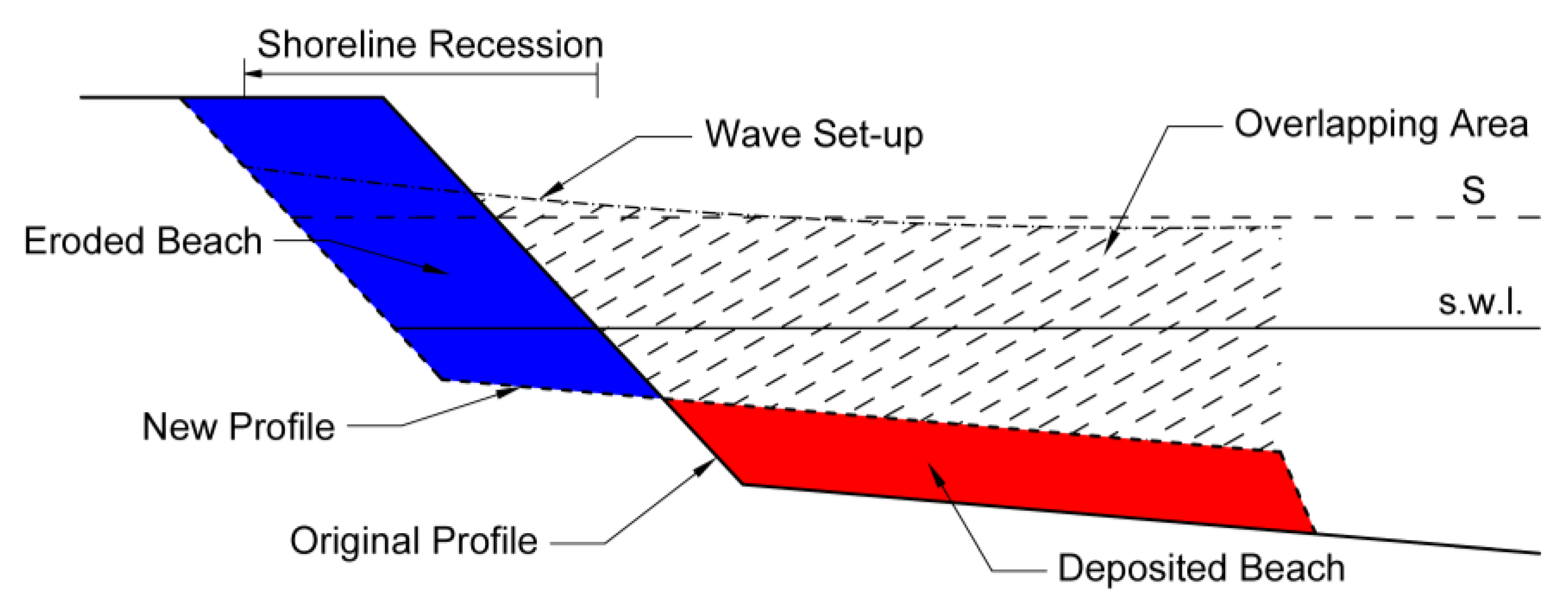
As an example, the visual representation of the terms contained in Equation (4) is reported in Figure 4. Here, the left-hand side of Equation (4) is given by the sum of the overlapping area and the blue area, while the right-hand side is given by the sum of the overlapping area and the red area. By subtracting the overlapping area, the blue and red areas are found, representing the final eroded and deposited volumes, respectively.
4. Results
In this section, the main results of the tests described in Section 3 are reported. For each beach profile, by the combinations of the different parameters of Table 1, 364 tests were carried out in the case of free beach, 54,600 for the beach protected by submerged breakwater, and 382,200 for the beach protected by emerged breakwater.
4.1. Free Beach
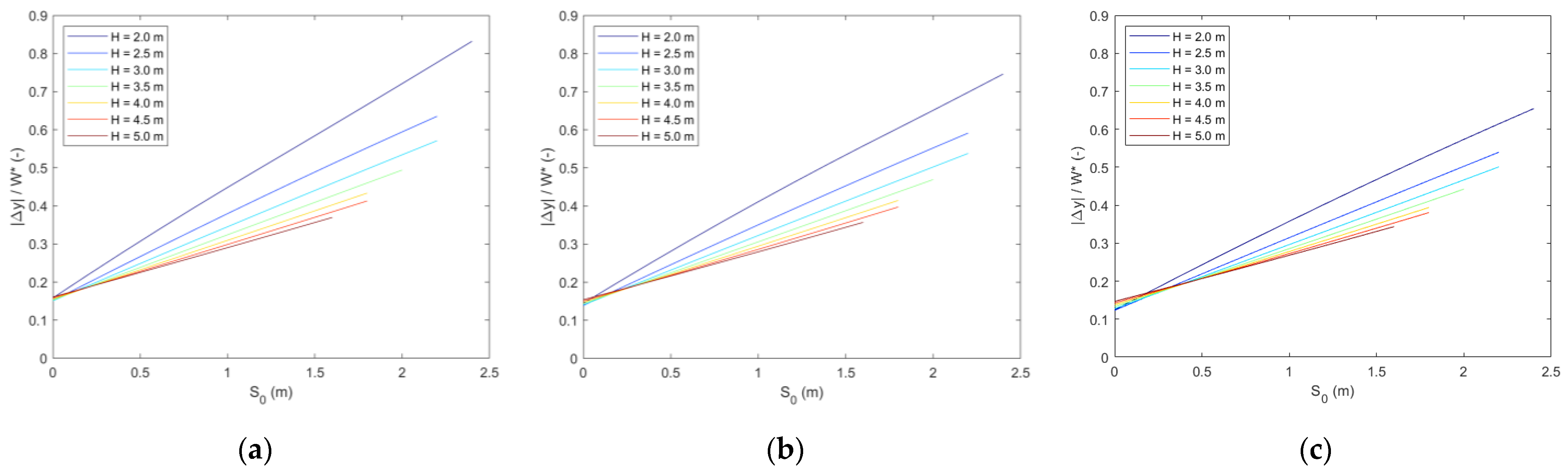
The analysis for the case of the unprotected free beach was conducted for three different slopes m (1/10, 1/20, 1/30) associated with the beach profile shown in Figure 3. In agreement with the dimensionless approach of [6,7], the results of the retreatment of the beach are shown in terms of the parameter Δy/W*. Here, for the chosen beach profile, the parameter W* was computed, according to its definition, as:
In panels of Figure 5, each line represents the dimensionless recession given by a specific wave height plotted as a function of the offshore sea level rise S0.
The analysis of the behavior of the parameter |Δy|/W* is not so direct and can lead to misinterpretations. Some common behaviors are evident in the three panels of Figure 5. As expected, given a specific wave height, the dimensionless erosion increases linearly with S0. Opposite to what should be expected, an increase in the value of H0 leads to a smaller |Δy|/W* for S0 larger than about 0.1 ÷ 0.3 m. This happens because of the presence of H0, m, and m0 in W* due to the shape of the chosen beach profile (Equation (11)). Note that by applying Equation (5), which is valid for the equilibrium beach profile and vertical berm, an increase in the values of the wave height leads to an increase in the ratio |Δy|/W*. However, such an increase becomes gradually smaller with the increase of S0. After a specific value of S0, the lines intersect, and an opposite behavior occurs. The decrease of the beach berm height, not shown in the paper, leads to a smaller value of S0 for which the cross point occurs.
As an example, for the values of H0 in Table 1, an increase in H0 of 0.5 m always leads to an increase in W* of about 64 m but, due to the steeper shoreward slope (e.g., 1/10), the value of W* changes from 76 m (H0 = 2.0 m) to 140 m (H0 = 2.5 m). Such effects become less relevant for the following increments of H0 due to the general increase in the total absolute value of W*. Although the analysis on a single beach slope would have removed this effect, the double beach slope profile better represents usual field conditions.
The slope angles of the lines in Figure 5 decrease with the increase of H0 and with the increase of the beach slope (Figure 5, from panels a to c). It must be highlighted that, for the equations used within the model, the wave period does not have any effect on beach erosion in the case of free beaches.
Following these preliminary considerations, a general model is set according to the following Equation (12):
where the coefficients ai are the constants of the equation.
By the application of a nonlinear least-squares solver and after rounding the main exponents, Equation (13) can be obtained:
It can be simplified as:
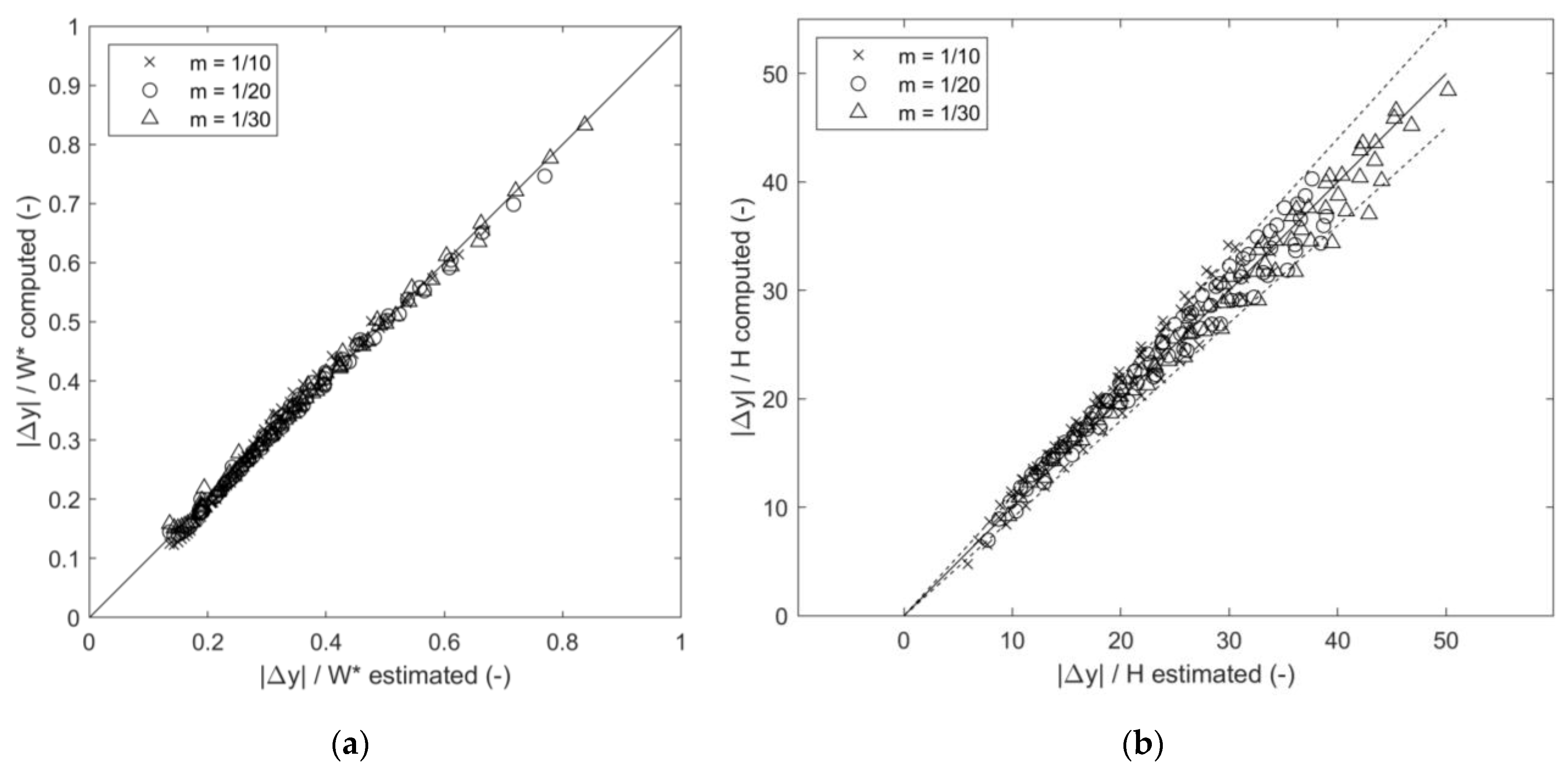
The coefficient of determination of Equation (14) is r2 = 0.993 and the goodness of its fit is reported in Figure 6a where the results of the model (y-axis) are plotted with respect to the results of Equation (14) (x-axis). The dimensionless retreat of the shoreline changes linearly with respect to S by a factor that decreases linearly with H0 and with the fourth root of m. When S0 = 0, Δy/W* varies with the fourth root of the dimensionless wave height (H0/Z).
In addition, with respect to Equation (5), Equation (14) takes into account the linear slope of the emerged beach, and it is also valid outside the condition Δy << W*. The latter condition is difficult to respect for steep beaches where the W* value decreases. Such extensions of the validity of the proposed model with respect to those available in the literature are noteworthy.
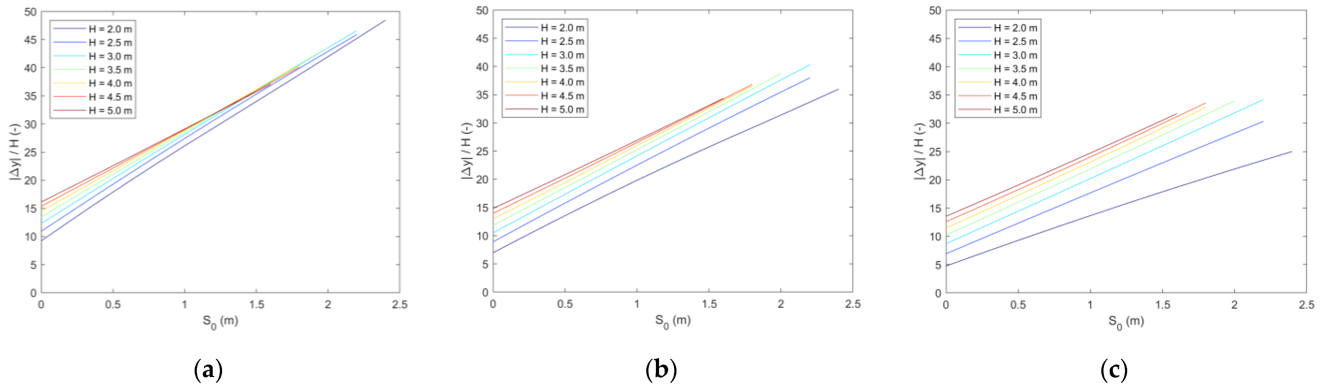
Although this formula gives excellent results, its interpretation is more complex due to the definition of W*. Therefore, a more practical approach is followed, with the analysis of the ratio Δy/H0. If the erosion is made dimensionless by H0 instead of W*, Figure 7 is obtained.
Here, the behavior seems to be in contrast with the results of Figure 5 where the dimensionless shoreline recession was decreasing with respect to the wave height. The reason for this difference stands in the already analyzed definition of W*. Here, this ambiguity is overcome, and the results better represent the tendency of the shoreline retreat.
The shoreline recession Δy is given by the sum of two contributions. The first contribution is purely geometric, due to the flood given by the increase of the sea level on a sloped beach (flooding contribution F) and it can be calculated as Δyf = −(S0 + 0.188H0)/m where the coefficient 0.188 represents the maximum water level due to the set-up according to Equation (3) for y = 0. The second contribution is that of the actual beach profile recession (erosive contribution E) and it depends on H0, S0, and m. Following the approach that leads to Equation (14), a general model is set:
Again, by the application of a nonlinear least-squares solver and after rounding the main exponents, Equation (16) can be obtained:
It can be simplified as:
where the dimensional equation for Δy becomes:
Equations (15)–(17) are associated with a coefficient of determination r2 = 0.970 and the results of their application with respect to the results of the numerical model are plotted in Figure 6b.
Equation (18) allows a better understanding of the dynamics of the recession of the shoreline due to waves and sea level rise for an unprotected beach. When H0 is constant, Δy increases linearly with S0, while a quadratic dependence from H0 is observed when S0 is constant. Finally, the presence of m in the denominators of the second and third terms of the right-hand side of Equation (18) means that for steeper beaches the shoreline recession decrease mostly due to the flooding effect. On the contrary, the contribution of m to the recession of the whole profile due to the erosion process is the opposite. If we only consider the second, third, and fourth terms of the right-hand side of Equation (16) that represent the actual erosion, the positive sign of the last term means that a steep beach is more eroded than a mild beach even if the final value of Δy is smaller. The same information is also implicitly included in Equation (14) because of the presence of m in the definition of W*. However, a superficial interpretation of such an equation could lead to a misinterpretation of the recession behavior of beaches with different slopes. The same ambiguity is also present in Equation (5) where W* is defined as (Hb/κA)3/2 where A is the shape parameter of the beach profile. Equation (18) allows a better understanding of the effects of the main hydro and morphodynamic quantities (H0, S0, m) on the shoreline recession.
4.2. Breakwaters
In the case of a beach protected by breakwaters, the results of emerged and submerged structures must be studied together because, mostly due to the sea level rise, emerged breakwater can become submerged (Point 4 of Section 3.1). Due to the large number of involved parameters, the analysis is structured as follows:
- In the first subchapters of the present section, the main effects of each parameter on the shoreline recession are studied. This is achieved by assigning a constant and typical value to the other parameters;
- Based on the considerations obtained from the previous point, a global behavior is then studied with respect to the free beach case.
4.2.1. Freeboard (Rc)
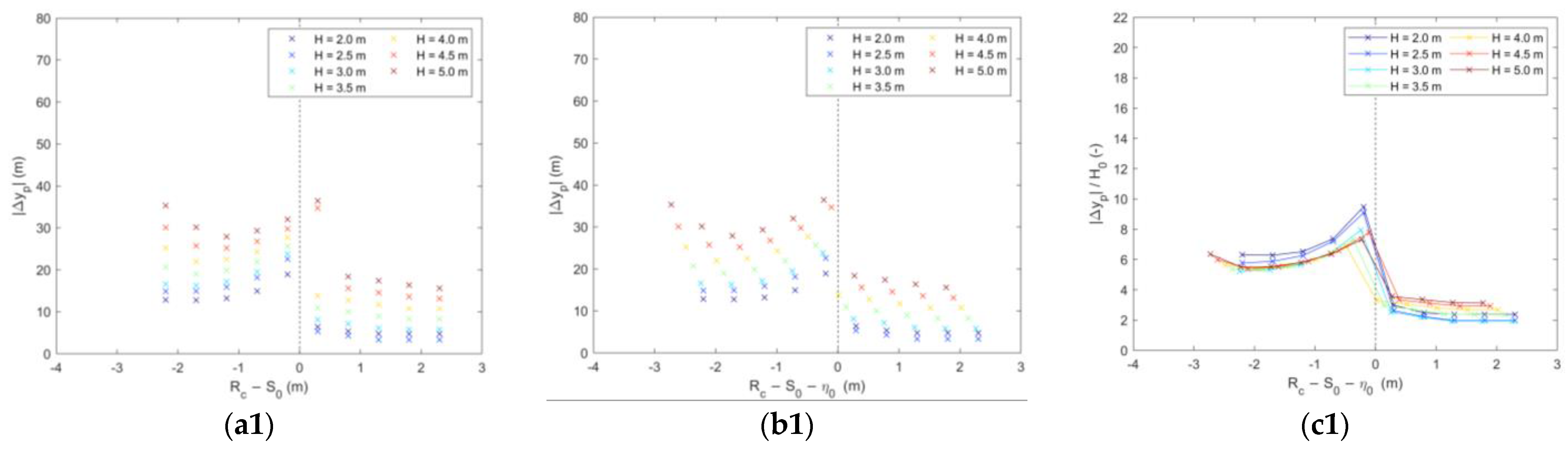
The main parameter that influences the behavior of a breakwater is the freeboard. According to this parameter, a structure can be submerged (Rc ≤ 0) or emerged (Rc > 0). However, when sea level rise occurs, the actual freeboard becomes Rc − S0. To highlight the role of these parameters, the shoreline recession results in the protected beach scenario (Δyp) as shown in Figure 8. Here, the first row is obtained for S0 = 0.2 m and the second row refers to S0 = 1.0 m. The breakwater is placed at the water depth ht = 3 m; the width of the berm is B = 8 m; the wave period is T = 9 s and the beach inner slope is m = 1/20. In each panel, seven different colors of markers are used, depending on the wave height (from dark blue to dark red when increasing the wave height). The results are first plotted as a function of Rc − S0 (panels a). Both for S0 = 0.2 m (a1) and for S0 = 1.0 m (a2), a drop in the shoreline recession is observed after a value of Rc ≈ S0 is reached. This drop is due to the fact that when the structure becomes submerged, a piling-up effect is considered, and hence, the final erosion is increased. However, the separation between emerged and submerged breakwaters can be improved. As an example, in Figure 8a1, the values of |Δyp| obtained for H0 = 4.5–5.0 m at Rc − S0 ≈ 0.2 m are wrongly associated with the emerged breakwater case. In fact, the largest waves break seaward with respect to the breakwater, and thus, the actual sea level has to be increased due to set-up effects.
From Equation (3), it is possible to evaluate such an effect by computing the value of (y) at ht. If κ is taken equal to 0.78 the offshore set-up () effect on the sea level rise can be calculated as:
The offshore set-up contribution to the sea level is only added if the wave breaking depth H0/κ is larger than the term ht + S0, when the offshore set-up is negative at the structure it is not considered in the computations for safety reasons. When the breaking occurs offshore of the structure, this contribution is added and the actual value of Rc,1 can be computed as Rc,1 = Rc − S0− , as shown in Figure 8b.
Here, for both tests with S0 = 0.2 m and S0 = 1.0 m the drop occurs exactly when Rc,1 = 0 m. This updated parameter is able to better characterize the behavior of the structure and it will be taken as a reference in further analysis.
For Rc,1 < 0 m, the breakwater is submerged. The piling-up plays the primary role and, because of its definition (Equations (8) and (9), a hyperbolic decrease of |Δyp| with Rc,1 is observed (see H0 = 2–3 m in Figure 8b1). For larger waves (e.g., H0 = 3–5 m in Figure 8b2), the contribution of the piling-up becomes less important for Rc,1 < −1 ÷ −2 m, where the effect of the wave transmission leads to larger values of the shoreline recession. For larger values of S0 with respect to those of Figure 8, a limit value of Δy is obtained due to the maximum constant value of the transmitted wave height that limits Equations (6) and (7).
For Rc,1 ≥ 0 m, the breakwater remains emerged. The shoreline response only depends on the wave transmission and, therefore, a linear behavior is observed between Rc,1 and Δyp.
If the shoreline recession of the protected beach is made dimensionless with the offshore wave height (|Δyp|/H0), Figure 8c is obtained. Here, for each wave height, also the line is added to the markers to follow better the behavior of each group. Figure 8c1,c2 show a minimum value of the dimensionless shoreline recession |Δyp|/H0 for submerged breakwaters that is associated with a value of Rc,1 of about −1.5 m for a typical berm width of 8 m. Therefore, knowing the design wave height H0 and, hence, the offshore set-up , the optimal breakwater submergence Rc can be defined for a specific sea level rise S0 scenario.
4.2.2. Effect of the Main Parameters (B, ht, T, and m)
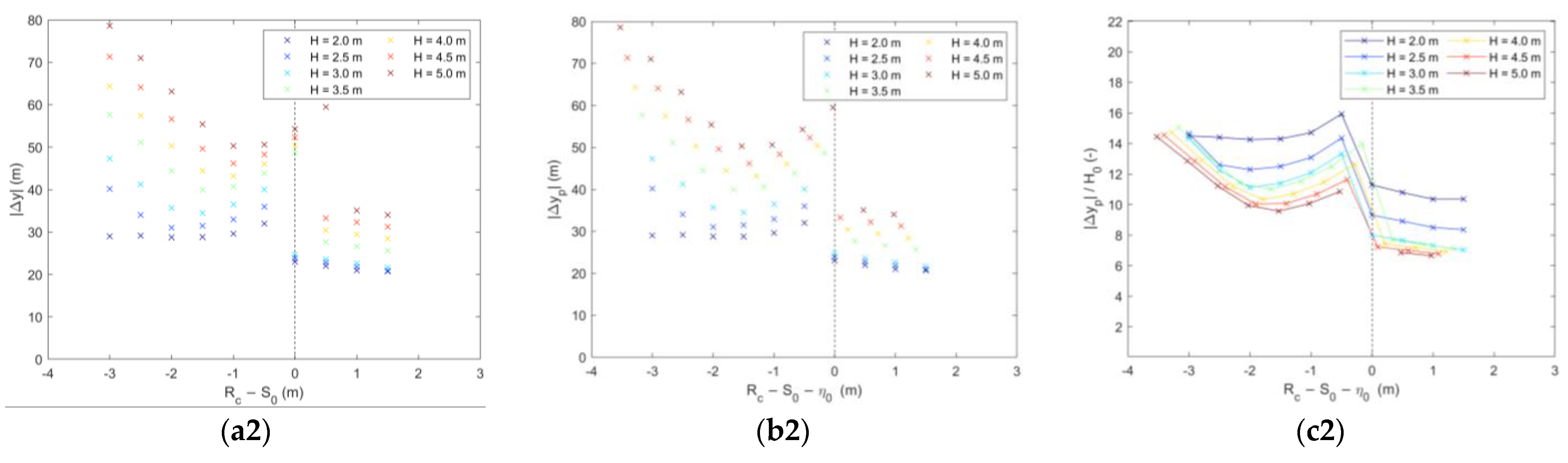
Among the geometric parameters of the breakwater, the width of the crest berm (B) plays a primary role. Such a parameter influences both the transmitted wave and the piling-up. Its effect on the reduction of the shoreline recession is shown in Figure 9a, obtained for H0 = 3 m, ht = 3 m, T = 9 s, m = 1/20 and for two different sea levels (panel a1 for S0 = 0.2 m and panel a2 for S0 = 1.0 m). A larger value of B reduces both the wave transmission and the piling-up. When the sea level increases (panel a2), the effect is more evident. When the structure becomes submerged and B is increased from 3 m to 8 ÷ 13 m, a strong reduction of the shoreline recession is obtained; further increase in this parameter leads to a smaller beneficial effect. In addition, as Rc,1 decreases, the growing trend of |Δyp|/H0 begins at higher values of Rc,1 with the decrease of B. If the structure remains emerged (Rc,1 > 0), an increase of B is also favorable for beach protection until the minimum value of kt is reached, leading to the horizontal line in panel a1. After this condition is reached, a further increase in Rc,1 does not lead to a reduction of |Δyp|/H0.
The water depth at the toe of the structure (Figure 9b) and the wave period (Figure 9c) showed a weaker influence on the shoreline. Figure 9b shows the results for varying values of ht and fixed values of H0 = 3 m, B = 13 m, T = 9 s, m = 1/20. For small values of S0 (panel b1), when ht increases, the dimensionless recession is larger if the breakwater is submerged while it is smaller if the structure remains emerged. When the sea level increases (panel b2), the effect of the increase of ht over a certain value is almost negligible. For ht = 2.5 m, the smallest tested water depth, a different behavior with respect to the others is observed because the wave breaks offshore to the structure thus increasing the mean water level by (y). Figure 9c shows the results for varying values of T and fixed values of H0 = 3 m, B = 13 m, ht = 3 m, m = 1/20. The wave period has a smaller effect, for emerged breakwaters, it can be considered negligible, while for submerged breakwaters, longer waves lead to larger piling-up and, thus, greater ratios |Δyp|/H0. This effect is more evident for larger values of S0.
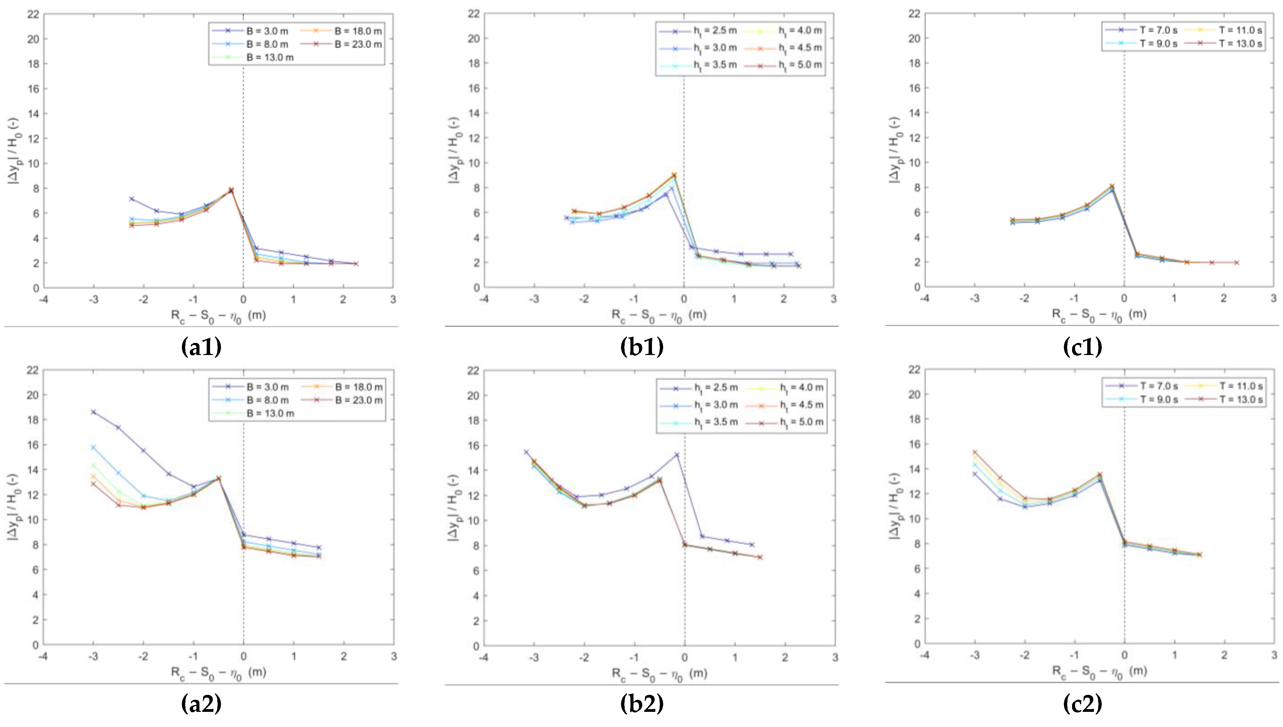
The inner slope of the beach (m) influences the results because of its presence in the definition of W* in Equation (11). In Section 4.1, the results for the free beach cases are always calculated in the condition that the wave breaking depth H0/κ is larger than the water depth hp. Here, the reduction of the wave height due to the presence of the breakwater can lead to the condition H0/κ < hp and, therefore, the horizontal limit of the integration W* decreases faster for lower values of H0 and this effect is enhanced by the slope m.
As a consequence, Figure 10 shows that for steeper beaches (larger m) the ratio |Δyp|/H0 is smaller. When the sea level increases (panel b) and the piling-up effect becomes negligible (Rc,1 < −2 m), only the wave transmission effect is present. Here, for steeper beaches, for decreasing values of Rc,1, the shoreline recession increases faster with respect to the case of milder beaches.
4.3. Shoreline Recession of Protected Beaches
As already pointed out in Section 4.2, the final shoreline recession in the presence of breakwaters is influenced by a large number of parameters. In this section, explicit relations for its evaluation are found. From the offshore hydrodynamic conditions, the wave heights and the water levels change due to the presence of the structure according to the explicit Equations (6) and (7) (Kt) and to the implicit Equations (8) and (9) (P0). The shoreline recession is hence obtained from the integration of Equation (4) with the updated hydrodynamic values. An explicit relation that accounts for all these effects would result in a very complex equation that may lead to unphysical meanings.
Therefore, to provide a practical and effective tool, some initial computations are needed. First, the set-up of the large offshore waves () is computed according to Equation (19). The wave height at the toe of the structure (H1) is hence computed as the minimum value between the offshore wave height (H0) and the maximum allowed wave height computed as Hmax = κ(ht + S0 + ). The actual value of the freeboard is computed (Rc,1 = Rc − S0 − ) and the transmission coefficient is calculated by the application of Equations (6) and (7) where the values of Rc,1, H1, L, and B are used. Depending on the value of Rc,1, two different scenarios are analyzed. If Rc,1 > 0, the breakwater keeps in emerged conditions, and no effect of piling-up is added; if Rc,1 ≤ 0, the breakwater is submerged and the piling-up is considered.
4.3.1. Emerged Breakwaters
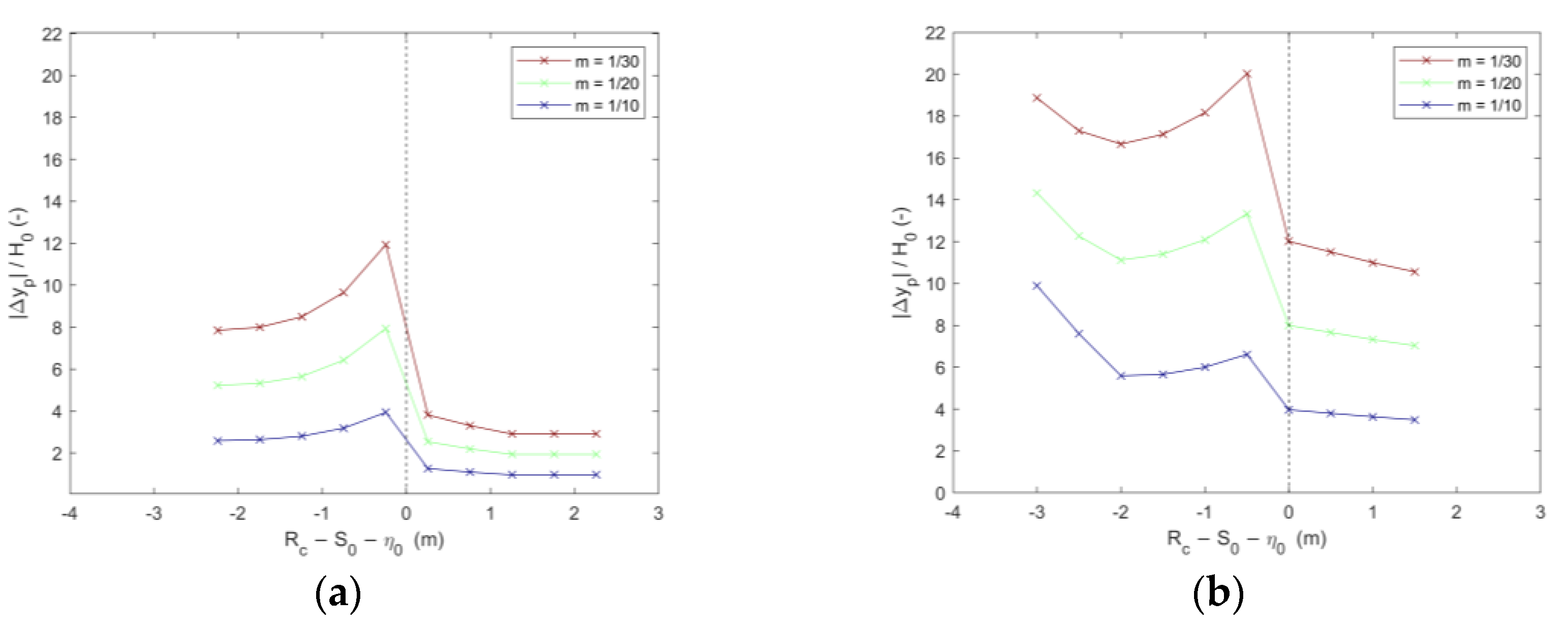
Following the approach of Equation (15), first, the flooding contribution F is computed by taking into account the updated values of water level and wave height. With respect to the free beach case, the reduced value of KtH1 leads to a smaller area in which the integration is performed and, therefore, the erosion contribution included in Δyp is smaller than the flooding one and becomes relevant only for large values of KtH1. Based on these assumptions, the following relation for the case of emerged breakwaters is obtained by considering the sum of two contributions: the flooding F, due to the increase of water level and the erosive contribution E, as reported in Equation (20). By collecting the flooding contribution F, the erosive part C1 can be obtained by finding the best-fit relation of the data:
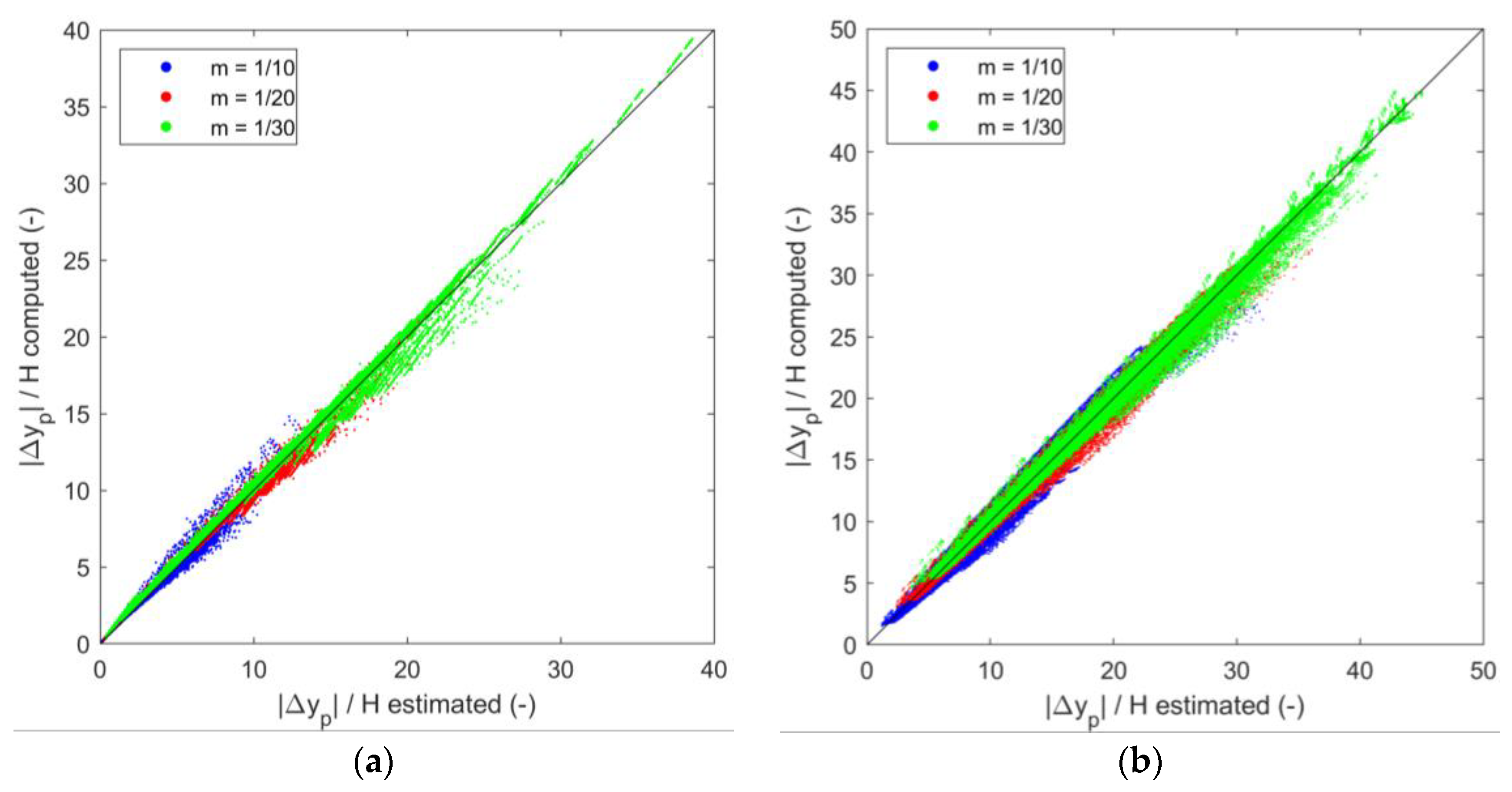
Here, in agreement with Kriebel et al. [10], the erosive contribution of C1 increases with the slope of the emerged beach m. The fitting of this equation with the results of the model is shown in Figure 11a in which the colors change with respect to the slope of the beach profile. Equation (20) leads to a coefficient of determination r2 = 0.997.
4.3.2. Submerged Breakwaters
If the breakwater is submerged (or it becomes submerged due to the sea level rise), the piling-up contribution plays an important role in the shoreline recession and it must be taken into account. Therefore, its effect must be added as an additional term in the flooding factor. According to the implicit Equations (8) and (9), the maximum value of P0 is obtained at Rc = 0 and it decreases with the submergence of the structure. If the value of hm0 is set to zero, the value of hm = P0/2 can be substituted in Equation (8), which can be solved for P0, obtaining:
Depending on the values of G calculated at the toe of the structure, Equation (21) can be rounded as follows:
This value represents the maximum value of piling-up computed for the zero freeboard case (Rc,1 = 0). P0 is found to decrease in a negative exponential form when increasing the submergence of the breakwater. By means of data fitting of the shoreline recession data from the model, the following approximate expression for piling-up computation is obtained:
Hence, the final dimensionless shoreline recession is calculated as the sum of the flooding F and the erosive contribution E. By collecting F, the erosive part C2 can be obtained by finding the best-fit relation:
The fitting of this equation with the results of the model is shown in Figure 11b in which the colors change with respect to the slope of the beach profile. Equation (24) leads to a coefficient of determination r2 = 0.992.
Equations (20) and (24) allow the estimation of the dimensionless shoreline recession for the protected beach case. The range of hydrodynamic conditions and breakwater characteristics reported in Table 1 is very wide and covers the majority of coastal environment conditions. However, it must be highlighted that such equations can be considered valid only within the range of the beach slope here tested. As an example, the application of Equation (24) with a value of m < 1/83 would lead to a factor (1−C2) smaller than unity which is something unphysical. In any case, the range of the emerged beach tested in the present study is large enough to represent the most typical field conditions.
5. Discussion and Conclusions
The correct management of coastal areas requires the knowledge of a large number of factors that are responsible for the beach erosion/accretion process. Bathymetric data and sediment distribution are needed as long as information about the wave climate, sediment supply from rivers, longitudinal/transversal sediment flowrate and direction, presence of man-made structures, and the expected values of sea level rise is available. Such kind of studies are usually carried out by the application of the so-called modeling cascade in which more detailed software are applied towards the shoreline. The need for limited computational time can lead to some assumptions, and therefore uncertainties, in the parameters/phenomena to be modeled. In addition, the presence of breakwaters requires the application of detailed wave phase-solving tools that usually cannot take into account all the phenomena. The present work provides a semi-analytical tool for a first estimate of the shoreline recession due to waves and sea level rise. With respect to the well-known analytical solution of Dean [7], some restrictions to the beach profile are overcome. The present method can be applied to any beach profile. In particular, in order to obtain results for common beach profile situations, a double slope beach profile is studied with an offshore slope of 1/100 and three different onshore slopes in the range of the expected field conditions (m = 1/10 ÷ 1/30). In addition, the restriction of the unrealistic vertical berm of the emerged beach (needed for the analytical computation) is removed. Finally, the presence of emerged/submerged breakwaters is taken into consideration in terms of wave height reduction and piling-up. Several hydrodynamic conditions and breakwater characteristics have been studied. In the first part of the paper, two equations are obtained by the interpolation of the model results for the estimation of the shoreline recession for the unprotected beach case. In Equation (14) the shoreline recession is made dimensionless with the breaker zone width W*. In Equation (17), instead, in order to give a more common parameter for coastal area management, the shoreline recession is made dimensionless with the offshore wave height. The presence of breakwaters is also studied. The breakwater freeboard influences significantly the shoreline recession mainly because, for large values of sea level rise, which can be due to climate change and storm surge, emerged breakwater can become submerged and its efficacy is reduced. For submerged structures, a minimum value of the dimensionless shoreline recession is found for values of effective freeboard equal to about −1.5 m with a typical berm width of 8 m. Therefore, knowing the hydrodynamic conditions (S0, H0), an optimal breakwater submergence Rc can be computed. The increase of the berm width leads to a considerable decrease in shoreline recession due to the reduction in terms of piling-up. However, such a reduction becomes almost negligible for B >10 m. The water depth where the breakwater is placed shows a weak influence. Although the erosive process increases with the slope of the emerged beach, milder slope beaches lead to larger values of shoreline recession due to the larger flooding contribution. Finally, based on the approach used for the free beach scenario, two prediction relations for the shoreline recession are found by fitting the model data for the case of emerged (Equation (20)) and submerged breakwaters (Equation (24)). The values of the coefficient of determination are very high (r2 ≥ 0.992), hence ensuring the goodness of the fitting equations studied within the very wide range of parameters reported in Table 1. The aim of the model is to provide information on the effect of waves and sea levels on beach recession in presence of breakwaters. It must be noted that the model is mainly based on empirical formulas and the final results are found to be coherent with the nature of the phenomena. However, future work is needed for the validation of the model with experimental or field data.
Author Contributions
Conceptualization, A.M., S.C., C.L., F.M., and S.R.; methodology, F.M. and S.R.; software, F.M.; formal analysis, S.R., F.M., and S.C.; investigation, F.M., S.R., and S.C.; data curation, F.M., S.R., and S.C.; writing—original draft preparation, F.M.; writing—review and editing, F.M., S.C., and S.R.; supervision, A.M., S.C., and C.L.; All authors have read and agreed to the published version of the manuscript.
Funding
This research received no external funding.
Data Availability Statement
Not applicable.
Conflicts of Interest
The authors declare no conflict of interest.
List of Symbols and Abbreviations
| α | inner and outer slope of the breakwaters |
| Δy | beach profile recession |
| Δyf | free beach profile recession |
| Δyp | beach profile recession in presence of breakwaters |
| (y) | wave set-up |
| offshore set-up | |
| wave set-down | |
| κ | breaking index |
| ξ | Iribarren parameter |
| A(d50) | scale parameter for equilibrium beach profile computation |
| B | width of the berm of the breakwaters |
| CVB | Calabrese-Vicinanza-Buccino method for piling-up computation |
| d50 | mean sediment diameter |
| Ed | energy dissipated by the breakwater |
| Ef | energy transmitted over the breakwater by filtration |
| Ei | incoming energy from waves |
| Eo | energy transmitted over the breakwater by overtopping |
| Er | energy reflected by the breakwater |
| G | parameter involved in piling-up computation |
| h* | breaking depth in the initial profile |
| h(y) | water depth at a distance y from the shoreline |
| hb | breaking depth in the final profile |
| hm | average water depth in the surf zone over the breakwater |
| hm0 | average water depth in the surf zone over the breakwater in absence of piling-up |
| hp | water depth at which the profile changes its slope |
| ht | water depth at the toe of the breakwater |
| H0 | offshore wave height |
| H1 | wave height at the toe of the structure |
| Hb | wave height at the breaker |
| Hi | incident wave height |
| Hmax | maximum allowed wave height at the toe of the structure |
| Hm0i | incident significant wave height |
| Ht | transmitted wave height |
| J | constant depending on the breaking parameter κ |
| k | wave number |
| Kt | transmission coefficient |
| L | wave length |
| Lg | width of the gap between two breakwaters |
| Ls | width of the breakwater |
| m0 | offshore slope of the beach profile |
| m | inner slope of the beach profile |
| P0 | static piling-up |
| approximate static piling-up | |
| Rc | freeboard of the breakwater |
| Rc,1 | effective freeboard of the breakwater |
| s.w.l. | still water level |
| S0 | offshore water level variation with respect to s.w.l. |
| S1 | water level variation at the toe of the structure |
| S | water level variation in correspondence with the shoreline |
| T | wave period |
| W* | distance of the breaking point from the shoreline |
| xb | horizontal distance between the breaking point on the slope of the breakwater and the seaward crest edge |
| y | distance from the shoreline |
| ys | distance of the breakwaters from the shoreline |
| Z | emerged beach berm height |
References
- IPCC. Climate Change 2021: The Physical Science Basis; Contribution of Working Group I to the Sixth Assessment Report of the Intergovernmental Panel on Climate Change; Cambridge University Press: Cambridge, UK, 2021. [Google Scholar]
- van Gent, M.R.A. Climate Adaptation of Coastal Structures. In Proceedings of the SCACR19—9th Short Course/Conference on Applied Coastal Research, Bari, Italy, 9–11 September 2019; pp. 1–8. [Google Scholar]
- Toimil, A.; Losada, I.J.; Nicholls, R.J.; Dalrymple, R.A.; Stive, M.J.F. Addressing the Challenges of Climate Change Risks and Adaptation in Coastal Areas: A Review. Coast. Eng. 2020, 156, 1860–1870. [Google Scholar] [CrossRef]
- Bruun, P. The Bruun Rule of Erosion by Sea-Level Rise: A Discussion on Large-Scale Two-and Three-Dimensional Usages. J. Coast. Res. 1988, 4, 627–648. [Google Scholar]
- Bruun, P. Sea-Level Rise as a Cause of Shore Erosion. J. Waterw. Harb. Div. 1962, 88, 117–130. [Google Scholar] [CrossRef]
- Bruun, P. Coast Erosion and the Development of Beach Profiles; US Beach Erosion Board: Washington, DC, USA, 1954; Volume 44. [Google Scholar]
- Dean, R.G. Equilibrium Beach Profiles: Characteristics and Applications. J. Coast. Res. 1991, 7, 53–84. [Google Scholar]
- Dean, R.G. Equilibrium Beach Profiles: US Atlantic and Gulf Coasts; Ocean engineering technical report, no. 12; Department of Civil Engineering and College of Marine Studies, University of Delaware: Newark, NJ, USA, 1977. [Google Scholar]
- Li, Y.; Zhang, C.; Chen, D.; Zheng, J.; Sun, J.; Wang, P. Barred Beach Profile Equilibrium Investigated with a Process-Based Numerical Model. Cont. Shelf Res. 2021, 222, 104432. [Google Scholar] [CrossRef]
- Kriebel, D.L.; Kraus, N.C.; Larson, M. Engineering Methods for Predicting Beach Profile Response. In Proceedings of the Coastal Sediments, New Orleans, LA, USA, 13–17 May 2007; pp. 557–571. [Google Scholar]
- Dean, R.G.; Houston, J.R. Determining Shoreline Response to Sea Level Rise. Coast. Eng. 2016, 114, 1–8. [Google Scholar] [CrossRef]
- Larson, M.; Kraus, N.C. SBEACH: Numerical Model for Simulating Storm-Induced Beach Change. Report 1. Empirical Foundation and Model Development; Coastal Engineering Research Center: Vicksburg, MS, USA, 1989. [Google Scholar]
- Roelvink, D.; Reniers, A.; van Dongeren, A.; de Vries, J.T.; McCall, R.; Lescinski, J. Modelling Storm Impacts on Beaches, Dunes and Barrier Islands. Coast. Eng. 2009, 56, 1133–1152. [Google Scholar] [CrossRef]
- Kobayashi, N. Coastal Sediment Transport Modeling for Engineering Applications. J. Waterw. Port Coast. Ocean. Eng. 2016, 142, 03116001. [Google Scholar] [CrossRef]
- Kit, E.; Pelinovsky, E. Dynamical Models for Cross-Shore Transport and Equilibrium Bottom Profiles. J. Waterw. Port Coast. Ocean. Eng. 1998, 124, 138–146. [Google Scholar] [CrossRef]
- Marini, F.; Mancinelli, A.; Corvaro, S.; Rocchi, S.; Lorenzoni, C. Coastal Submerged Structures Adaptation to Sea Level Rise over Different Beach Profiles. Ital. J. Eng. Geol. Environ. 2020, 1, 81–92. [Google Scholar]
- Dean, R.G.; Dalrymple, R.A. Coastal Processes with Engineering Applications; Cambridge University Press: Cambridge, UK, 2004. [Google Scholar]
- Bowen, A.; Inman, D.; Simmons, V. Wave ‘Set-down’and Set-Up. J. Geophys. Res. 1968, 73, 2569–2577. [Google Scholar] [CrossRef]
- van der Meer, J.W.; Briganti, R.; Zanuttigh, B.; Wang, B. Wave Transmission and Reflection at Low-Crested Structures: Design Formulae, Oblique Wave Attack and Spectral Change. Coast. Eng. 2005, 52, 915–929. [Google Scholar] [CrossRef]
- Lara, J.L.; Garcia, N.; Losada, I.J. RANS Modelling Applied to Random Wave Interaction with Submerged Permeable Structures. Coast. Eng. 2006, 53, 395–417. [Google Scholar] [CrossRef]
- Zhang, C.; Li, Y.; Zheng, J.; Xie, M.; Shi, J.; Wang, G. Parametric Modelling of Nearshore Wave Reflection. Coast. Eng. 2021, 169, 103978. [Google Scholar] [CrossRef]
- Buccino, M.; Calabrese, M. Conceptual Approach for Prediction of Wave Transmission at Low-Crested Breakwaters. J. Waterw. Port Coast. Ocean. Eng. 2007, 133, 213–224. [Google Scholar] [CrossRef]
- Zanuttigh, B.; Martinelli, L. Transmission of Wave Energy at Permeable Low Crested Structures. Coast. Eng. 2008, 55, 1135–1147. [Google Scholar] [CrossRef]
- Briganti, R.; van der Meer, J.; Buccino, M.; Calabrese, M. Wave Transmission Behind Low-Crested Structures. In Proceedings of the Coastal Structures 2003, Portland, OR, USA, 26-30 August 2003; pp. 580–592. [Google Scholar] [CrossRef]
- d’Angremond, K.; van der Meer, J.; De Jong, R.J. Wave Transmission at Low-Crested Structures. In Proceedings of the ICCE, Orlando, FL, USA, 2–6 September 1996; pp. 3305–3318. [Google Scholar]
- Archetti, R.; Gaeta, M.G. Design of Multipurpose Coastal Protection Measures at the Reno River Mouth (Italy). In Proceedings of the International Offshore and Polar Engineering Conference, Sapporo, Japan, 10–15 June 2018; pp. 1343–1348. [Google Scholar]
- Soldini, L.; Lorenzoni, C.; Piattella, A.; Mancinelli, A.; Brocchini, M. Nearshore Macrovortices Generated at a Submerged Breakwater: Experimental Investigation and Statistical Modeling. In Proceedings of the 29th International Conference on Coastal Engineering, Lisbon, Portugal, 19–24 September 2004; pp. 1380–1392. [Google Scholar] [CrossRef]
- Lorenzoni, C.; Mancinelli, A.; Postacchini, M.; Mattioli, M.; Soldini, L.; Corvaro, S. Experimental Tests on Sandy Beach Model Protected by Low-Crested Structures. In Proceedings of the 4th International Short Conference on Applied Coastal Research (SCACR), Barcelona, Spain, 15–17 June 2009; pp. 310–322. [Google Scholar]
- Calabrese, M.; Vicinanza, D.; Buccino, M. 2D Wave Set up behind Low-Crested and Submerged Breakwaters. In Proceedings of the 3th International Offshore and Polar Engineering Conference, Honolulu, HI, USA, 25–30 May 2003; pp. 831–836. [Google Scholar]
- Calabrese, M.; Vicinanza, D.; Buccino, M. 2D Wave Setup behind Submerged Breakwaters. Ocean. Eng. 2008, 35, 1015–1028. [Google Scholar] [CrossRef]
- Kamphuis, J.W. Incipient Wave Breaking. Coast. Eng. 1991, 15, 185–203. [Google Scholar] [CrossRef]
- Battjes, J.A.; Stive, M.J.F. Calibration and Verification of a Dissipation Model for Random Breaking Waves. J. Geophys. Res. 1985, 90, 9159. [Google Scholar] [CrossRef]
- Apotsos, A.; Raubenheimer, B.; Elgar, S.; Guza, R.T. Testing and Calibrating Parametric Wave Transformation Models on Natural Beaches. Coast. Eng. 2008, 55, 224–235. [Google Scholar] [CrossRef] [Green Version]
- Zhang, C.; Li, Y.; Cai, Y.; Shi, J.; Zheng, J.; Cai, F.; Qi, H. Parameterization of Nearshore Wave Breaker Index. Coast. Eng. 2021, 168, 103914. [Google Scholar] [CrossRef]
Figure 1.
Profile geometry and notation for shoreline recession due to waves and increased water level (adapted from [17]).
Figure 1.
Profile geometry and notation for shoreline recession due to waves and increased water level (adapted from [17]).

Figure 2.
Sketch of the most relevant design characteristics of emerged (Rc > 0) or submerged (Rc < 0) rubble-mound breakwater in a vertical cross-section (left panel) and in a plan view (right panel).
Figure 2.
Sketch of the most relevant design characteristics of emerged (Rc > 0) or submerged (Rc < 0) rubble-mound breakwater in a vertical cross-section (left panel) and in a plan view (right panel).

Figure 3.
Sketch of the main parameters used in the integration.

Figure 4.
Example of the result of the integration for a beach profile protected by submerged breakwater. Blue area: eroded volume of beach; red area: deposited volume of beach. The left-hand and right-hand sides of Equation (4) are given by the sum of the dashed overlapping area with, respectively, the eroded or the deposited volume.

Figure 5.
Dimensionless erosion (|Δy|/W*) for free beaches with different slopes: (a) m = 1/30; (b) m = 1/20; (c) m = 1/10.
Figure 5.
Dimensionless erosion (|Δy|/W*) for free beaches with different slopes: (a) m = 1/30; (b) m = 1/20; (c) m = 1/10.

Figure 6.
Results of the dimensionless beach profile erosion obtained with the model with respect to Equation (14) (r2 = 0.993; panel (a)) and Equation (17) (r2 = 0.970; panel (b)).
Figure 6.
Results of the dimensionless beach profile erosion obtained with the model with respect to Equation (14) (r2 = 0.993; panel (a)) and Equation (17) (r2 = 0.970; panel (b)).

Figure 7.
Dimensionless erosion (|Δy|/H0) for free beaches with different slopes: (a) m = 1/30; (b) m = 1/20; (c) m = 1/10.
Figure 7.
Dimensionless erosion (|Δy|/H0) for free beaches with different slopes: (a) m = 1/30; (b) m = 1/20; (c) m = 1/10.

Figure 8.
Absolute (|Δyp|) and relative shoreline recession (|Δyp|/H0) for beaches protected by breakwaters for 2 different values of sea level rise: (a1–c1) for S0 = 0.2 m; (a2–c2) for S0 = 1.0 m. (a1,a2) absolute recession with respect to Rc − S0; (b1,b2) absolute recession with respect to Rc − S0 − ; c1, c2 relative recession with respect to Rc − S0 − . Constant values: B = 8 m, ht = 3 m, T = 9 s, m = 1/20.


Figure 9.
Relative shoreline recession (Δyp/H0) for beaches protected by breakwaters for 2 different values of sea level rise: (a1–c1) for S0 = 0.2 m; (a2–c2) for S0 = 1.0 m. (a1,a2) dependence from B, constant values: H0 = 3 m, ht = 3 m, T = 9 s, m = 1/20. (b1,b2) dependence from ht, constant values: H0 = 3 m, B = 13 m, T = 9 s, m = 1/20. (c1,c2) dependence from T, constant values: H0 = 3 m, B = 13 m, ht = 3 m, m = 1/20.

Figure 10.
Relative shoreline recession (|Δyp|/H0) for beaches protected by breakwaters for 2 different values of sea level rise: (a) for S0 = 0.2 m; (b) for S0 = 1.0 m. Dependence from m, constant values: H0 = 4 m, B = 8 m, ht = 3 m, T = 9 s.
Figure 10.
Relative shoreline recession (|Δyp|/H0) for beaches protected by breakwaters for 2 different values of sea level rise: (a) for S0 = 0.2 m; (b) for S0 = 1.0 m. Dependence from m, constant values: H0 = 4 m, B = 8 m, ht = 3 m, T = 9 s.

Figure 11.
Comparison between |Δyp|/H0 computed by the model and |Δyp|/H0 computed with best-fit equations in presence of emerged breakwaters (panel (a), Equation (20), r2 = 0.997) and submerged breakwaters (panel (b), Equation (24), r2 = 0.992).
Figure 11.
Comparison between |Δyp|/H0 computed by the model and |Δyp|/H0 computed with best-fit equations in presence of emerged breakwaters (panel (a), Equation (20), r2 = 0.997) and submerged breakwaters (panel (b), Equation (24), r2 = 0.992).


Table 1.
Summary of the tested values for each parameter.
| H0 (m) | T (s) | S0 (m) | ht (m) | Rc (m) | B (m) | m (-) |
|---|---|---|---|---|---|---|
| 2.0:0.5:5.0 | 7:2:13 | 0:0.2:2.4 | 2.5:0.5:5.0 | −2.0:0.5:2.5 | 3:5:23 | 1/10; 1/20; 1/30 |
Publisher’s Note: MDPI stays neutral with regard to jurisdictional claims in published maps and institutional affiliations. |
© 2022 by the authors. Licensee MDPI, Basel, Switzerland. This article is an open access article distributed under the terms and conditions of the Creative Commons Attribution (CC BY) license (https://creativecommons.org/licenses/by/4.0/).
Share and Cite
MDPI and ACS Style
Marini, F.; Corvaro, S.; Rocchi, S.; Lorenzoni, C.; Mancinelli, A. Semi-Analytical Model for the Evaluation of Shoreline Recession Due to Waves and Sea Level Rise. Water 2022, 14, 1305. https://doi.org/10.3390/w14081305
AMA Style
Marini F, Corvaro S, Rocchi S, Lorenzoni C, Mancinelli A. Semi-Analytical Model for the Evaluation of Shoreline Recession Due to Waves and Sea Level Rise. Water. 2022; 14(8):1305. https://doi.org/10.3390/w14081305
Chicago/Turabian StyleMarini, Francesco, Sara Corvaro, Stefania Rocchi, Carlo Lorenzoni, and Alessandro Mancinelli. 2022. "Semi-Analytical Model for the Evaluation of Shoreline Recession Due to Waves and Sea Level Rise" Water 14, no. 8: 1305. https://doi.org/10.3390/w14081305
Note that from the first issue of 2016, this journal uses article numbers instead of page numbers. See further details here.