
Monitoring the Chl-a Distribution Details in the Yangtze River Mouth Using Satellite Remote Sensing


Marine Science and Technology College, Zhejiang Ocean University, Zhoushan 316004, China
*
Author to whom correspondence should be addressed.
Water 2022, 14(8), 1295; https://doi.org/10.3390/w14081295
Submission received: 22 March 2022
/
Revised: 13 April 2022
/
Accepted: 13 April 2022
/
Published: 15 April 2022
(This article belongs to the Special Issue Eutrophication Management in Coastal Zones for Better Water Quality)
Abstract
:The distribution of chlorophyll-a (Chl-a) in the Yangtze River Mouth area was analyzed using a new Chl-a inversion model (PMS-C) based on the relationship between in situ Chl-a and GF-4 PMS band combinations. Combining GF-4 PMS with HY-C CZI, this paper revealed that: (1) Chl-a concentration in Yangtze River Mouth was in the range of 2–6 µg/L, being higher in the west than in the east. The high Chl-a area was mainly distributed near the mouth of the Yangtze River and the Chl-a value was in the range of 3.7 µg/L to 5.9 µg/L. Chl-a concentration is higher in spring and summer than in autumn and winter, with a Chl-a concentration difference of 1–2 µg/L. Chl-a downstream of islands and bridges increased by 0.5–1.7 µg/L compared with upstream. (2) Short-term (within 3 h) changes of Chl-a concentration were effectively detected. In summer and autumn, Chl-a obtained at 13:30 in the noon was generally lower than Chl-a obtained at around 10:30 in the morning and it decreased by nearly 0.1–4 μg/L within three hours on the same day. In winter, the concentration of Chl-a decreased in the range of 0–1.9 μg/L. Generally, within three hours, Chl-a in the downstream of the island decreased significantly from 5 μg/L to about 3.8 μg/L, and Chl-a downstream of piers decreased from 3.7 μg/L to about 3 μg/L. (3) Environmental factors including seawater temperature, illumination, and nutrients, as well as dynamic factors such as wind and tidal current can induce Chl-a change in the Yangtze River Mouth. Short-term change of Chl-a concentration is closely related to the specific hydrodynamic conditions, nutrients, and lighting conditions.
1. Introduction
Estuaries are places where the river meets the ocean. They are important natural areas where the continents and oceans exchange energy and various materials [1]. The phenomena of industrialization and urbanization are a great hazard to water quality. Agricultural activities and excessive fertilization of domestic waste can lead to eutrophication of water [2,3]. In addition, researchers point out that climate change has become increasingly severe and unstable, which will ultimately affect water and nutrient cycles, especially in vulnerable areas such as estuaries. A series of studies in recent years show that due to human activities and climate change, the estuary’s water quality is gradually deteriorating [4]. Therefore, monitoring suspended sediment distribution, Chl-a concentration, and other water environment factors, identifying their temporal and spatial dynamics, and describing their influencing factors and their interaction mechanisms are of great significance to estuarine water quality management [5].
As the largest river mouth in China, the Yangtze River Mouth carries about 108 t of sediment in to the sea. Pollutants in these sediments contain various nutrients of phytoplankton such as N, P, and Si [6]. The special hydrological conditions of the Yangtze River Mouth make it a water area that is very sensitive to water dynamics and climate change as well as human activities and pollution [7]; these factors can ultimately induce the change of water environment parameters such as Chl-a. Water in the Yangtze River Mouth and its adjacent area belongs to typical type II water [8], which is dominated by many optical factors including suspended particulate matter (SPM), colored dissolved organic matter (CDOM), and phytoplankton and their decomposing detritus [9,10]. Chl-a, a photosynthetic pigment commonly contained in various phytoplankton, is a good indicator of the biomass of marine phytoplankton [11]. Chl-a concentration in marine water is one of the important water quality parameters for marine environment detection [12].
Satellite remote sensing is a more robust monitoring tool that can be used to map the temporal and spatial changes of water quality factors such as Chl-a [13,14], compared with field observation which is time-consuming and costly. Based on satellite remote sensing, many studies have been performed, focusing on Chl-a monitoring in type II water such as Yangtze River Mouth and Bohai Bay [15]. Type II water is affected by terrigenous material and human activity; thus, it has a complicated water composition. In addition, blue and green wavelengths of reflectance ratio also depend on the perfection of the atmospheric correction models, but the absorption of aerosol in the blue band will make for a larger category of water body of atmospheric correction effect [16]. These problems have drawn the attention of many scholars [17]. Given the former problem, many scholars proposed to use red and near-infrared bands to avoid the above defects of blue-green bands in the inversion algorithm of type II water bodies [11,12,18,19,20]. In addition to the traditional two-band ratio method, some scholars have proposed a three-band algorithm for the medium muddy water [21]. This kind of algorithm introduces new bands to weaken the influence of CDOM and suspended particles in the water body on remote sensing reflection [22].
Many studies have focused on Chl-a detection based on satellite data. Dairolmo et al. used a three-band algorithm to analyze the influence of phytoplankton and Chl-a light emission quantum yield on the inversion results and found that the specific absorption coefficient may be the most important factor affecting the accuracy of the inversion algorithm [19]. Gitelson et al. [17,23] used a three-band algorithm established by Moderate-Resolution Imaging Spectroradiometer (MERIS) and a two-band algorithm established by Moderate-Oriented Deposit Insurance Scheme (MODIS) to retrieve the Chl-a concentration of type II water, respectively, and found that the correlation coefficients with the Chl-a concentration were 0.96 and 0.92, respectively. Chl-a in the Yellow Sea and East China Sea [23] was retrieved using an empirical algorithm to invert Chl-a concentration and it was detected that the uncertainty of Chl-a was up to 35%. The hyperspectral reflectance of 653 nm, 691 nm, and 748 nm, and the hyperspectral remote sensing data of HuanJing-1A (HJ-1A) satellite 656 nm, 716 nm, and 753 nm were applied to perform the three-band algorithm to retrieve the Chl-a concentration of Dian Shan Lake. This indicates that the hyperspectral remote sensing data of the HJ-1A satellite can be used for Chl-a concentration inversion and water status monitoring of type II water bodies. Furthermore, many scholars have also carried out studies on remote sensing watercolor inversion. Thematic Mapper (TM) data and quasi-synchronous data, as well as MODIS, were adopted to study the Chl-a concentration of Taihu Lake and Bohai Sea; researchers found that normalized vegetation index (NDVI) contributes to Chl-a inversion [24]. To reduce the influence of suspended particles in high-muddy isolated water on the fluorescence height algorithm, prior researchers applied 560 nm, 670 nm, and 620 nm to establish the Synthetic Chlorophyll Index (SCI) In Leaves Index to extract Chl-a [3]. Meanwhile, field measurement data were applied [25] in the previous empirical algorithm model to obtain the watercolor factor of the Yellow and East China Sea. Chl-a concentration in the Yangtze Mouth was analyzed based on the ratio of blue-green bands constructed by MERIS [26]. Red, near-infrared (NIR), blue, and green bands of GaoFen-1 satellite wide field of view (GF-1/WFV) data [27] were also applied to analyze Chl-a in Yangtze Mouth. Since the inversion correlation of water with high turbidity in the Yangtze Mouth is not particularly high (R2 > 0.9), we need to establish a more perfect model to invert Chl-a concentration in the Yangtze Mouth.
The GF-4 geosynchronous optical satellite is currently the world’s highest-resolution earth observation satellite in geostationary orbit [28,29]. Its continuous monitoring can make up for the shortcomings of traditional reconnaissance satellites such as low time resolution and small coverage area [30]. At the same time, it will introduce some new application areas, including ground-based traversal capabilities [31]. In addition, it has fast response capabilities, shortening the transmission time of user applications to geospatial information to a few minutes [32]. It is also capable of moving target monitoring, real-time monitoring, and upgrading satellite reconnaissance function to monitoring function [30]. Therefore, developing a suitable Chl-a model for the Yangtze River Mouth based on GF-4 data is necessary.
In this paper, a new Chl-a model was developed based on PMS data from GF-4 satellite and field data, and the concentration distribution of Chl-a in the Yangtze Mouth is analyzed. Detailed changes in Chl-a concentration over a short period (3 h) are analyzed using the advantage of continuous observations by geostationary orbiting satellites.
2. Data and Methods
2.1. Study Area
The Yangtze River Mouth is distributed in the coastal area of eastern China and is backed by Shanghai and Jiangsu, China, and faces the East China Sea, forming a trumpet shape area (Figure 1) [33]. The Yangtze River is more than 6300 km long and it is the longest river in China. The South Branch is divided into North Channel and South Channel by Changxing Island. In addition, Jiuduansha divides the South Channel into South Passage and North Passage, forming the characteristics of three branches and four ports entering the sea (Figure 1) [8]. Along with the enormous runoff in the Yangtze River Basin, the sediment pouring into the sea annually from the Yangtze River Mouth can reach up to 486 million tons on average [34]. Due to the interannual and seasonal variations of runoff, the sediment transport rate has apparent changes [35]. In July, the sediment transport rate is about 32 times that of January and the sediment transport during the flood season accounts for 87% of the total sediment transport [36]. The sediment from the Yangtze River Mouth is mainly scattered in the southeast direction. Under the combined action of runoff and tidal current, a large amount of sediment is deposited near the entrance of the South Branch. The underwater delta outside the opening of the South Branch is the main deposition area. In the vicinity of the interception point outside the Mouth, suspended sediment stays for a long time, forming a maximum turbidity zone, and the suspended sediment concentration drops sharply at 122.5° E [37]. Therefore, we position the longitude of the study area as 120.5–122.5° E.
2.2. Satellite Data
2.2.1. GF-4 Data
The GF-4, which uses array gaze imaging, has the ability to detect visible and infrared wavelengths; it entered service on 13 June 2016 [38]. The designed life of GF-4 is eight years, pointing to the particular region and performing observation in China and surrounding areas [19]. With 36,000 km orbital altitude and resolution of fifty meters, GF-4, together with the previously launched GF-1 and GF-2 satellites operating in low orbit, forms a constellation with the advantages of high temporal resolution and high spatial resolution [39]. GF-4 fills in the gap of China’s and even the world’s high-orbit high-resolution satellites [40]. The spectral response function can be obtained on the website of the China Resources Satellite Application Center. The satellite data (PMS-L1A) are derived from the China Center for Resources Satellite Data and Application (http://www.cresda.com, accessed on 15 March 2021). The information of GF-4 PMS sensor was shown in Table 1.
2.2.2. HY-1C/CZI Data
China launched the HaiYang-1C (HY-1C) satellite on the LM-2C carrier rocket [41]; it monitors the global ocean color and water temperatures, providing services for the development and utilization of marine organism [41]. The Coastal Zone Imager (CZI) carried by HY-1C has a spatial resolution of 50 m and a spectral range of 421–500 nm, 517–598 nm, 608–690 nm, and 761–891 nm [42]. It can be networked with other similar loads to form a higher observation capacity [35]. CZI sensor parameters and image information are shown in Table 2.
2.3. Collection of Water Samples and Laboratory Analysis
In situ measurement was performed from 307 stations in the Yangtze River Mouth at about 10:30 a.m. on 18 August 2020. Water samples were collected and Chl-a value was measured (Figure 1a), from which 174 measured data were applied to establish the inversion formula, and the remaining 133 data were prepared for verification.
Chl-a data were obtained by filtering 100–500 mL of water through a glass fiber filter and recording the volume of the filtered water sample. Steps were as follows: add enough 90% acetone solution to drown the filter paper, record the volume, plug the plug, and put the filter paper at 4 °C for 4 h out of light. If cloudy, centrifugal extraction can be performed. Part of the extract was poured into a 1 cm glass test tube, a cuvette cap was added, and the absorbance at 665 nm and 750 nm was measured respectively based on the reagent blank. Next, add 1 drop of 2 mol/L hydrochloric acids into the two test tubes and mix for 1 min. Measure the absorbance at 665 nm and 750 nm, respectively [19,43].
2.4. Data Pre-Processing
2.4.1. Geometric Correction
GF-4 satellite data (Table 2) pre-processing was performed following the steps in previous study [19]. Atmospheric correction [44] was performed using FLAASH [45,46].
Orthographic correction methods mainly include two categories: one is a strict geometric correction model, the other is an approximate geometric correction model. When the imaging model and related parameters of remote sensing image are known, the image can be corrected according to the strict imaging model [47], which belongs to the strict geometric correction, and the collinear equation method is the most representative one [19]. However, when the sensor imaging model is unknown or the relevant auxiliary parameters cannot be obtained, the assumed mathematical model can be used to simulate the imaging model and realize image correction and this method belongs to approximate geometric correction, mainly including geometric polynomial correction, rational function method, local area correction, and other models [48].
The Rational Polynomial Coefficient (RPC) model expresses the image point coordinate D (line, sample) as the ratio of the ground point geodetic coordinate D (Latitude, Longitude, Height) and the independent variable [49]. In order to reduce the rounding error in the calculation process and enhance the stability of the parameter solution, it is necessary to regularize the ground coordinates and image coordinates between −1 and 1. In the RPC model, the first-order polynomial represents the distortion error model caused by optical projection, the second-order polynomial can approximate the distortion caused by earth curvature, projection refraction, lens tilt, and other factors, and the third-order polynomial can be applied to simulate other unknown distortions in the higher-order part [50]. The RPC conformal correction module in ENVI was applied for correction, and the error is controlled within 0.5 pixels in this paper.
2.4.2. Normalized Difference Water Index (NDWI)
In this paper, an adaptive extraction method based on NDWI was used to extract water completely and accurately from remote sensing images. The calculation formula for the NDWI is:
where GREEN and NIR are the value of the green band and the near-infrared band, respectively. The purpose of this indicator is to minimize the reflectivity of near-infrared light, while also making full use of the characteristics of plants and soil to enhance the reflectivity of water. Water properties are positive, while values for plants and soil are generally 0 or negative [51,52].
2.4.3. Model Evaluation
In this paper, regression analysis was performed to construct the model expression between the combination of bands and the concentration of water quality parameters. Therefore, R2, F test value, and the P-value of significance level were analyzed to evaluate the accuracy and robustness of the regression model. Meanwhile, to evaluate the accuracy of the model, the Root Mean Square Error (RMSE) was obtained using the predicted and measured values of the model [2]. The RMSE calculation method is as follows:
where y is the measured water quality parameter concentration, y′ is the simulated water quality parameter concentration, and n is the sample number.
2.5. SSC Retrieval
According to the empirical formula [35], based on the HY-1C/CZI data, the suspended sediment concentration (SSC) of the Yangtze River Mouth was retrieved using the red band and the NIR band. The formula is as follows:
where the unit of SSC is mg/L, and RRED and RNIR are the remote-sensing reflectance of the third (red) band and the fourth (NIR) band after atmospheric correction.
SSC = 64.54 − 7033.83 × RRED + 96027 × RNIR,
2.6. Tidal Current, Topography, and Wind
The Finite-Volume Community Ocean Model (FVCOM) [53,54] was performed for numerical simulation, and the tidal current was simulated every three hours on 30 November 2020. Considering the complex topography in the Yangtze Mouth, topographic data from the 1 Minute Gridded Global Relief Data Collection (ETOPO1) were obtained and analyzed. The resolution of ETOPO1 data is as high as 1 ‘×1’ and includes ice surface and bedrock, so it can better reflect the seabed topography.
The current is simulated with a hydrodynamic model, the FVCOM [53,54]. It is a popular ocean numerical model for estuaries and continental shelves. This model is an ocean numerical model of unstructured grid, finite volume method, free surface, and three-dimensional original equation jointly developed by UMASSD and WHOI [55,56]. FVCOM model used a finite volume algorithm to absorb the flexibility and the geometry of the finite element method and finite difference method of calculation efficiency. Apart from its advantage of simple structure, it can also fit complex coastline perfectly while ensuring the efficiency of calculation and guarantee the conservation of mass, momentum, temperature, and salinity in the process of calculation of a complex area. The model adapts unstructured grids to discretize the horizontal computing area and uses σ coordinates to fit the complex seabed topography vertically. Smagorinsky turbulence closure model [57] was used for horizontal mixed calculation of the mode, while Mellor–Yamada Order 2.5 turbulence closure model was used for vertical mixed calculation. The mode is similar to Princeton (POM). The external model is based on CFL condition and gravity wave velocity, and uses a shorter time step. It is a positive pressure model based on the two-dimensional vertical average equation. The internal model is based on CFL condition and internal wave velocity, and uses a longer time step. It is a baroclinic die based on three-dimensional equations. The three-dimensional global simulation results of the Hybrid Coordinate Ocean Model (HYCOM) reanalysis field were used for the initial temperature and salinity field, and the temperature, salinity, and flow field required by the open boundary of the model and the atmospheric forcing field were obtained from cfSR-V2 reanalysis field.
The terrain data are based on the global DEM data released by GEBCO in 2020 with a resolution of 15 s (http://mds.nmdis.org.cn, accessed on 11 May 2021). The wind field data are derived from the ERA-Interim dataset (https://www.ecmwf.int, accessed on 11 May 2021), one of many datasets produced by the ECMWF through a series of projects. The data include wind, temperature, rainfall, snow, and sea ice, which studies show have better accuracy than other meteorological data [58].
Monthly mean wind field data provided by the European Centre for Medium-Range Weather Forecasts (ECMWF) with a resolution of 0.125° × 0.125° was selected for the study area. ECMWF wind field data are representative of current high-precision weather forecast products [59]. MODIS SST Product (MOD28) is an ocean 3-level standard data product with a spatial resolution of 1 km [60]. The data source is NASA’s Ocean Water Color Data website (http://Oceancolor.gsfc.nasa.gov, accessed on 20 May 2021). SSS data were obtained using Hybrid Coordinate Ocean Model (HYCOM) monthly mean global high-resolution ocean assimilation data with a longitude level resolution of 1/12° [61]. These data were developed by the US Naval Research Laboratory using HYCOM; they use Multi-Variable Optimal Interpolation assimilation (MVOI), and assimilate available satellite altimeter observations, which are obtained along orbit through NAVOCEANO Altimeter Data Fusion Center [62].
3. Results
3.1. A New Chl-a Inversion Model for GF-4
3.1.1. Sensitive Band of Chl-a
To effectively identify Chl-a features, the bands should be selected according to the characteristics of the spectral curve features of Chl-a and the characteristic wavelengths of their absorption and reflection peaks [13,63]. Therefore, the correlation analysis (Figure 2) was performed using the remote sensing reflectance of 450–900 nm and the Chl-a concentration value obtained from 174 stations. The near-infrared (NIR) band (761–891 nm) highly correlated with Chl-a concentration, with R2 of 0.8681. However, due to the high concentration of SSC in high turbidity water of the Yangtze River Mouth, it is not suitable for Chl-a concentration inversion by using the NIR band. Beyond the NIR band, the coefficient of determination of the blue band (450–520 nm), green band (520–600 nm), and red band (608–690 nm) is 0.0970, 0.4067, and 0.6178, respectively, indicating that the correlation between the reflectance of these single bands and Chl-a concentration is generally very low. Therefore, the single band is not suitable to be considered as an independent variable to establish the Chl-a inversion model and band combination should be considered [19].
3.1.2. Model Establishment
Three different bands (B2, B3, B4) were randomly combined to analyze their correlation with Chl-a, and statistical analysis was carried out on variables (combination of band reflectance and measured Chl-a concentration) [64,65]. The R2 values of 60 band combinations in this paper range from 0.0108 to 0.9087, and the highest correlation of the single band combination is 0.8462. Eight combinations with R2 ≥ 0.8462 were selected, and its regression equation and corresponding R2 value are shown in Table 3.
The combined band with the highest R2 is the sixth combination in Table 3 marked by ★, indicating it is the optimal inversion model. Therefore, a new Chl-a inversion model (named PMS-C) for the coastal waters of the Yangtze Mouth was finally confirmed as Formula (5):
where the reflectance of band 2 (blue) was marked as Rrs(B2), the reflectance of band 3 (green) was marked as Rrs(B3), and the reflectance of band 4 (red) was marked as Rrs(B4).
ρ = 66.27 x2 − 14.751 x + 3.3302,
x = (Rrs(B3) − Rrs(B4))/(Rrs(B2) + Rrs(B3)),
The coefficients of determination (Figure 3) were analyzed to test the applicability of the newly built model and they made a particularly significant result with R2 = 0.9123, RMSE = 0.1752 µg/L, indicating that the modeled result is highly consistent with the in situ value. Therefore, the new model is suitable for GF-4 to retrieve Chl-a in coastal waters near the Yangtze Mouth.
3.2. Chl-a Analysis in Yangtze River Mouth
3.2.1. Chl-a Distribution
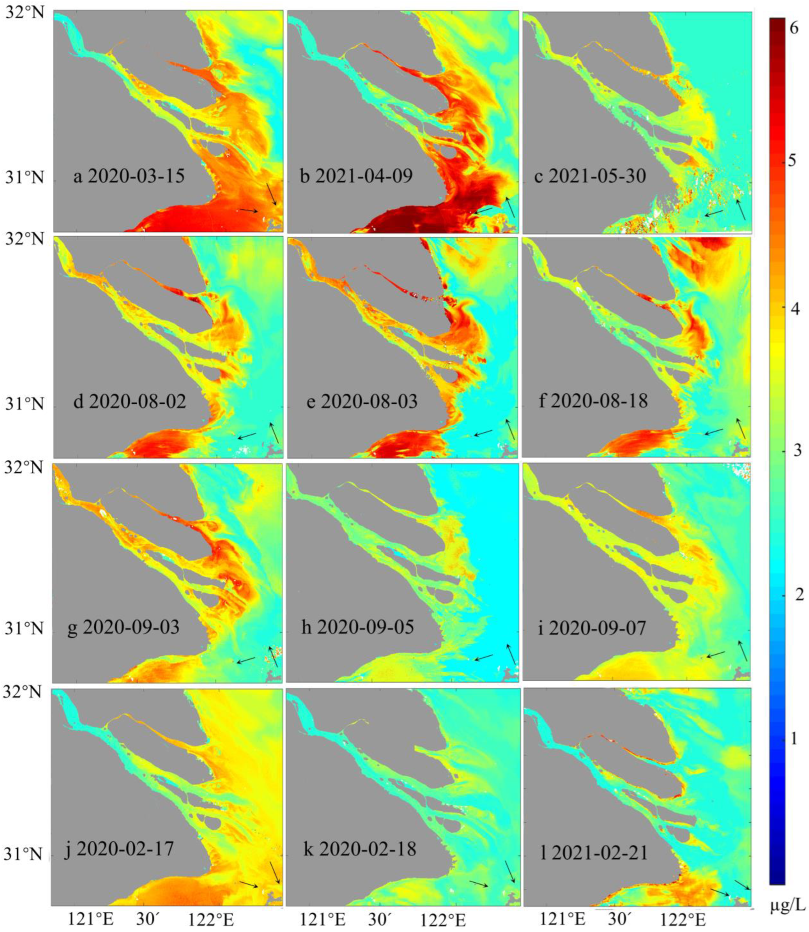
The distribution of Chl-a in the study area from February 2020 to May 2021 (Figure 4) was obtained using the newly built model PMS-C. The Chl-a concentration in Yangtze River Mouth is between 2 µg/L and 6 µg/L (Figure 4), and it is relatively high along the Yangtze River. In the mouth of the Yangtze River, where water depth is mainly less than 10 m (shallow area), the Chl-a value is in the range of 3.7 µg/L to 5.9 µg/L. The area with low Chl-a concentration is distributed outside the mouth of the Yangtze River, where the water depth is deeper than 20 m, and the value mainly ranges from 2.1 µg/L to 3.8 µg/L. The Chl-a concentration changes with the tidal current, obviously. During flood time (Figure 4b–i), the area with high Chl-a concentration was distributed in the northwest mouth of Yangtze River (Figure 4b–i) as well as inside the Yangtze River. During ebb tide (Figure 4a,j–l), the high Chl-a concentration area shifted to the southeast (green ellipse in Figure 4a,j–l) as a whole, consistent with the direction of the current.
Furthermore, the surface Chl-a in Yangtze Mouth shows a seasonal variation (Figure 4). In spring and summer, the concentration of Chl-a was high, ranging from 3 to 6 µg/L (Figure 4a–f). In autumn and winter (Figure 4g–l), the concentration of Chl-a was relatively low, ranging from 2 to 4 µg/L, and the Chl-a concentration gap between spring and autumn (Figure 4a–f) difference is about 1–2 µg/L. Chl-a concentration in the east is lower than that in the west and gradually decreased from the inside to the outside of the Yangtze River (Figure 4g–l). In the southwest of the Yangtze Mouth near Hangzhou Bay, Chl-a concentration is higher in spring and summer, but lower in autumn and winter.
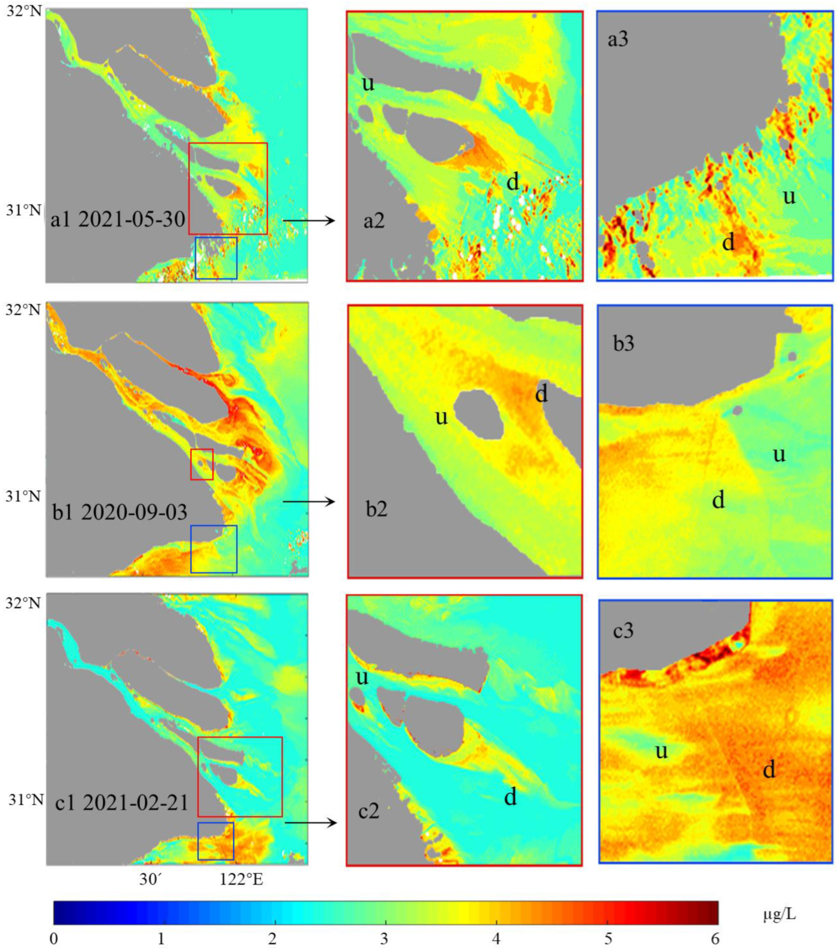
The direction of the bridge and island facing the water flow is defined as upstream (u) and the direction facing away from the water flow is defined as downstream (d). The downstream Chl-a concentration is generally higher than the upstream Chl-a concentration (Figure 5) with the gap in the range of 0.5–1.7 µg/L, indicating the difference between increased Chl-a value downstream and the original Chl-a value upstream. Take Chl-a on 21 February 2021, as an example (Figure 5c1–c3); Chl-a upstream of the island was 2.1 µg/L and it increased to nearly 3.8 µg/L downstream; the Chl-a gap is 1.7 µg/L. A similar rule also plays in Figure 5a1,a2, showing that when the tidal current flows through the island and bridge, no matter whether during the flooding period or ebbing period (Figure 5), the downstream Chl-a concentrations increased significantly.
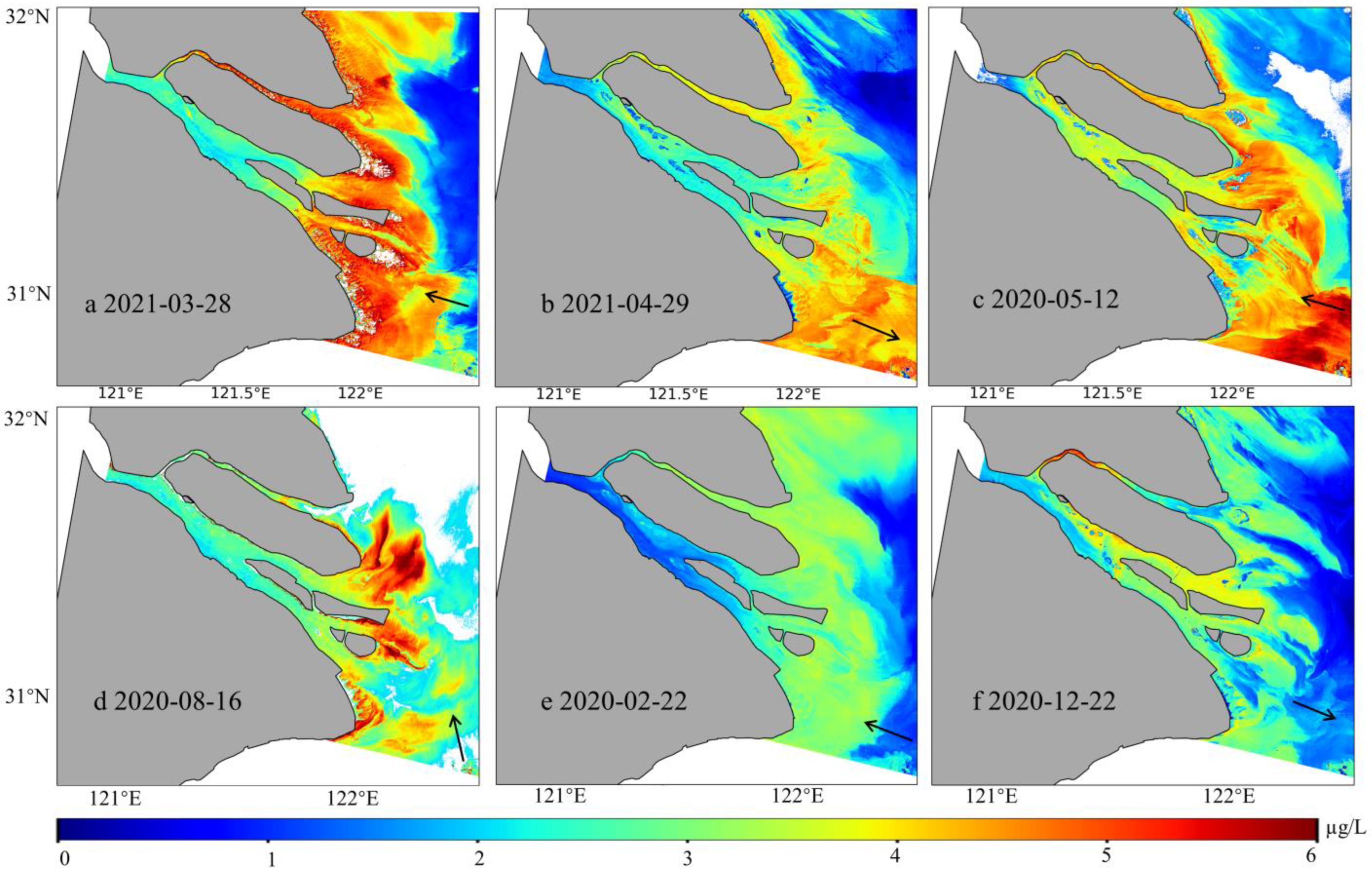
In order to further compare the Chl-a in the study area retrieved using our GF-4 model, the Chl-a from February 2020 to March 2021 obtained from Landsat 8-OLI Chl-a production data was analyzed (Figure 6). Generally, the high Chl-a area distributes in the middle of the Yangtze River Mouth and south of the Yangtze River Mouth near the Hangzhou Bay, ranging from 3 to 6 µg/L. The low Chl-a area distributes in the area outside the mouth of the Yangtze River, ranging from 0 to 2 µg/L. Furthermore, Chl-a concentration changes with the tidal current. When the tidal current flows eastward (ebbing), there is a large amount of Chl-a in the central part of the mouth area of the Yangtze River. Focusing on the waters near the island (Figure 6), it can be found that the downstream Chl-a increased no matter whether during flooding period or ebbing period, with Chl-a increased by 1–2 µg/L, and it also showed a higher concentration of Chl-a in spring and summer than in autumn and winter. Generally, the distribution and variation rule of Chl-a presented by Landsat 8-OLI satellite data are consistent with GF-4, which further demonstrates the feasibility of our GF-4 model.
3.2.2. Chl-a’s Short-Term (within Three Hours) Changes in Yangtze River Mouth
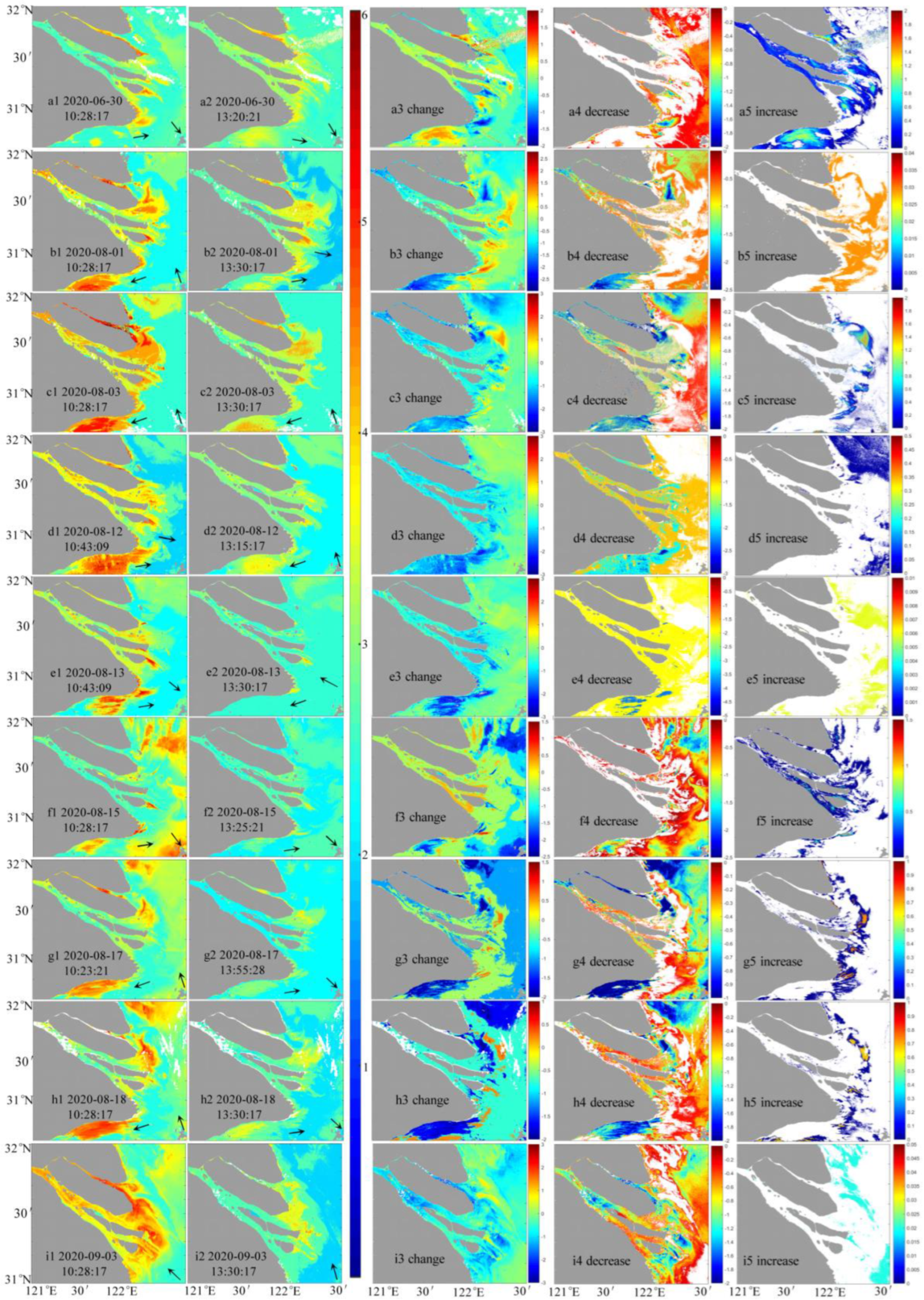
The GF-4 satellite in geostationary orbit can detect short-term changes of Chl-a concentration in detail. In this paper, we selected the data at different times in one day in summer and autumn, respectively, to detect the Chl-a change details in a short time (within 3 h). In summer and autumn (Figure 7), Chl-a concentration obtained at around 13:30 at noon is generally lower than Chl-a concentration obtained at around 10:30 in the morning and it decreased by around 0.1–4 μg/L within three hours on the same day.
Within 3 h of continuous ebb tide, the water flows away from the Yangtze Mouth to the southeast, Chl-a concentration decreased by about 0.2–1.5 μg/L in the east of the Yangtze Mouth (Figure 7a1,a2,f1,f2). Among them, the downstream of islands decreased significantly (about 0.6–1.8 μg/L) (Figure 7a4,f4), and on the contrary, the concentration of Chl-a increased slightly in the Yangtze Mouth, with the concentration increasing by around 0.1 μg/L. During the period of continuous flooding tide, the water flows into the Yangtze Mouth to the northwest (Figure 7c1,c2,i1,i2), Chl-a concentration in most areas of the Yangtze Mouth shows Chl-a decreased from 10:30 to 13:30, and the Chl-a decreased by 0.2–2 μg/L (Figure 7c4,i4), with only a few increased areas (Figure 7c5,i5). Meanwhile, when the tidal current changes from flood tide to ebb tide (Figure 7b1,b2,g1,g2,h1,h2) or from ebb tide to flood tide (Figure 7d1,d2,e1,e2) within three hours, Chl-a concentration at noon also decreased obviously compared with that in the morning. Only a few areas in the northeast and southeast of Yangtze River Mouth showed a slight increase.
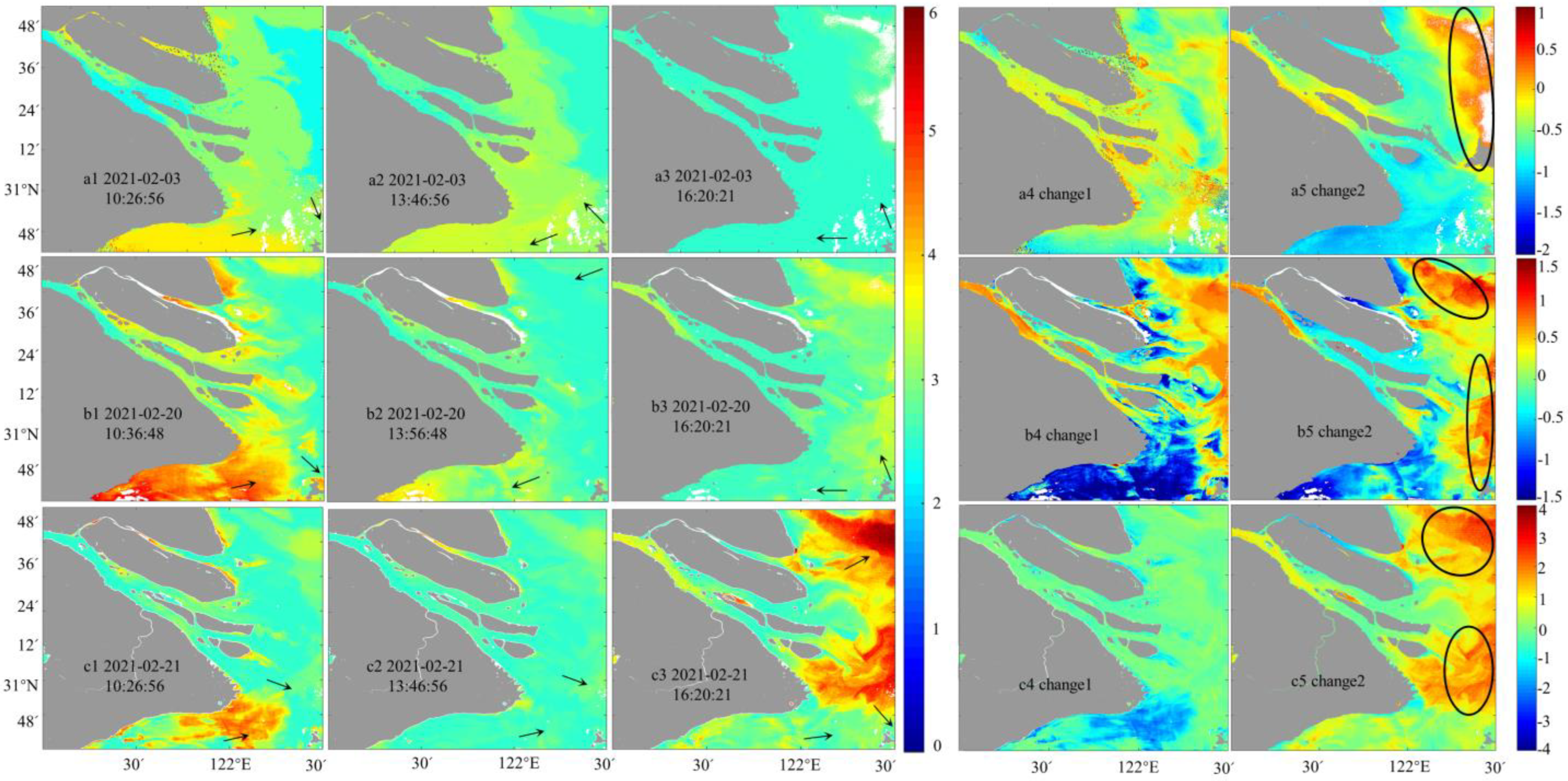
In winter (Figure 8), the distribution of Chl-a obtained in the morning and at noon has no obvious variety regularity. Compared with Chl-a in the morning, Chl-a can increase (Figure 8a4) or decrease (Figure 8b4,c4) at noon in the Yangtze River Mouth. From 13:30 to 16:30 in the afternoon, the east part of the Yangtze Mouth (black ellipse in Figure 8a5,b5,c5) showed an obvious increase, and the Chl-a concentration in other areas showed no obvious change.
3.3. SSC Retrieval Based on HY-1C
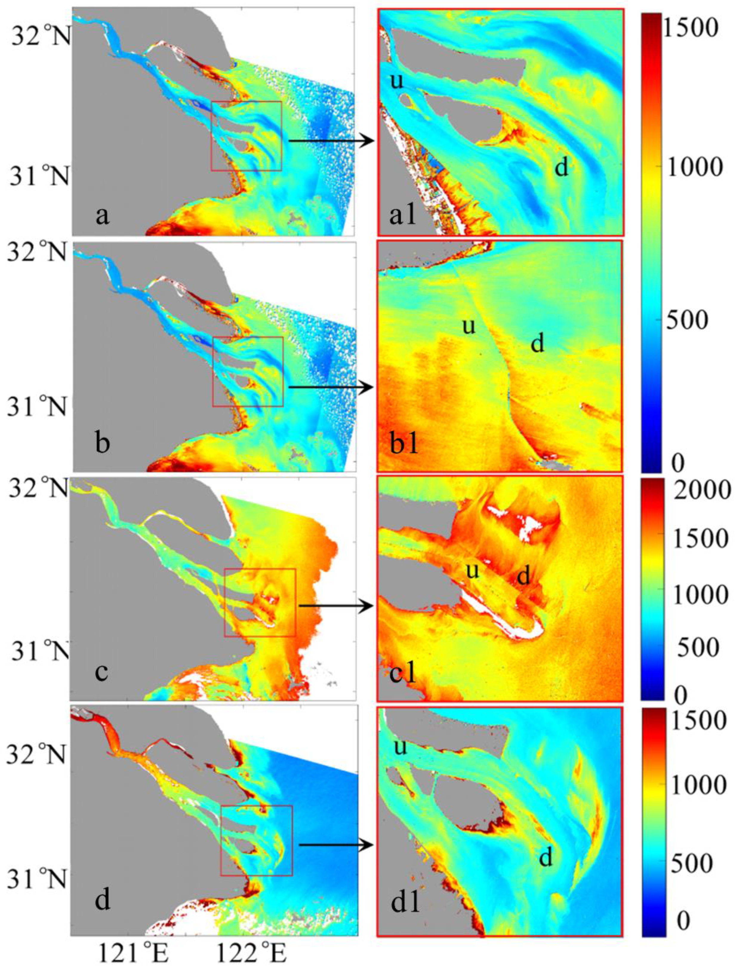
Generally, SSC is high with the value mainly in the range of 230–1700 mg/L and there is a great difference within the mouth area of the Yangtze River (Figure 9). The high SSC area is located in the middle of the Yangtze River Mouth and south of the Yangtze River Mouth near the Hangzhou Bay, with the SSC ranging from 900 to 1700 mg/L. The low SSC area is distributed in the area outside the mouth of the Yangtze River, with the SSC ranging from 450 to 1300 mg/L. Furthermore, SSC changes with the tidal current. When the tidal current flows eastward (ebbing), there is a large amount of suspended sediment in the central part of the mouth area of the Yangtze River. Focusing on the waters near the island (Figure 9a,d), it can be found that the downstream SSC increases, which is the same trend as Chl-a concentration. SSC increased downstream of islands, no matter whether during flooding period or ebbing period, with SSC increased by 300–600 mg/L.
4. Discussion
4.1. Applicability of the PMS-C Model
GF-4, China’s first civilian high-resolution geostationary optical satellite which has the highest resolution of any geostationary orbit satellite in the world, can be used for coastal ocean environment observation [30]. The bands selected to build the Chl-a inverse model are consistent with prior studies [7,66]. Yangtze Mouth and Hangzhou Bay’s Chl-a concentration were analyzed using MODIS satellite’s different bands; among them, near-infrared band and red band both achieved good simulation results [28]. Furthermore, the band ratio of blue and red bands was adopted to establish the model of inverse Chl-a concentration of Poyang Lake [13]. The band combination based on blue, green, and red band shows good availability, with R2 being 0.9142. The modeled results’ new model is suitable for the inversion of the type II water bodies in the Yangtze Mouth. The Chl-a distribution obtained using the newly established model in coastal waters near the Yangtze Mouth has a high consistency with in situ Chl-a as well as prior studies [2,4,7,13,67,68], indicating that this new model is suitable for Chl-a retrieval in this area.
4.2. The Factors Influencing Chl-a Concentration Distribution in the Study Area
The Chl-a variation in the Yangtze Mouth is induced by many environmental factors including temperature, light, nutrition, salinity [67], and dynamic factors induced by vertical movement of seawater [68]. These factors jointly affect distribution of Chl-a [18].
4.2.1. Factors Inducing Short-Term Changes of Chl-a
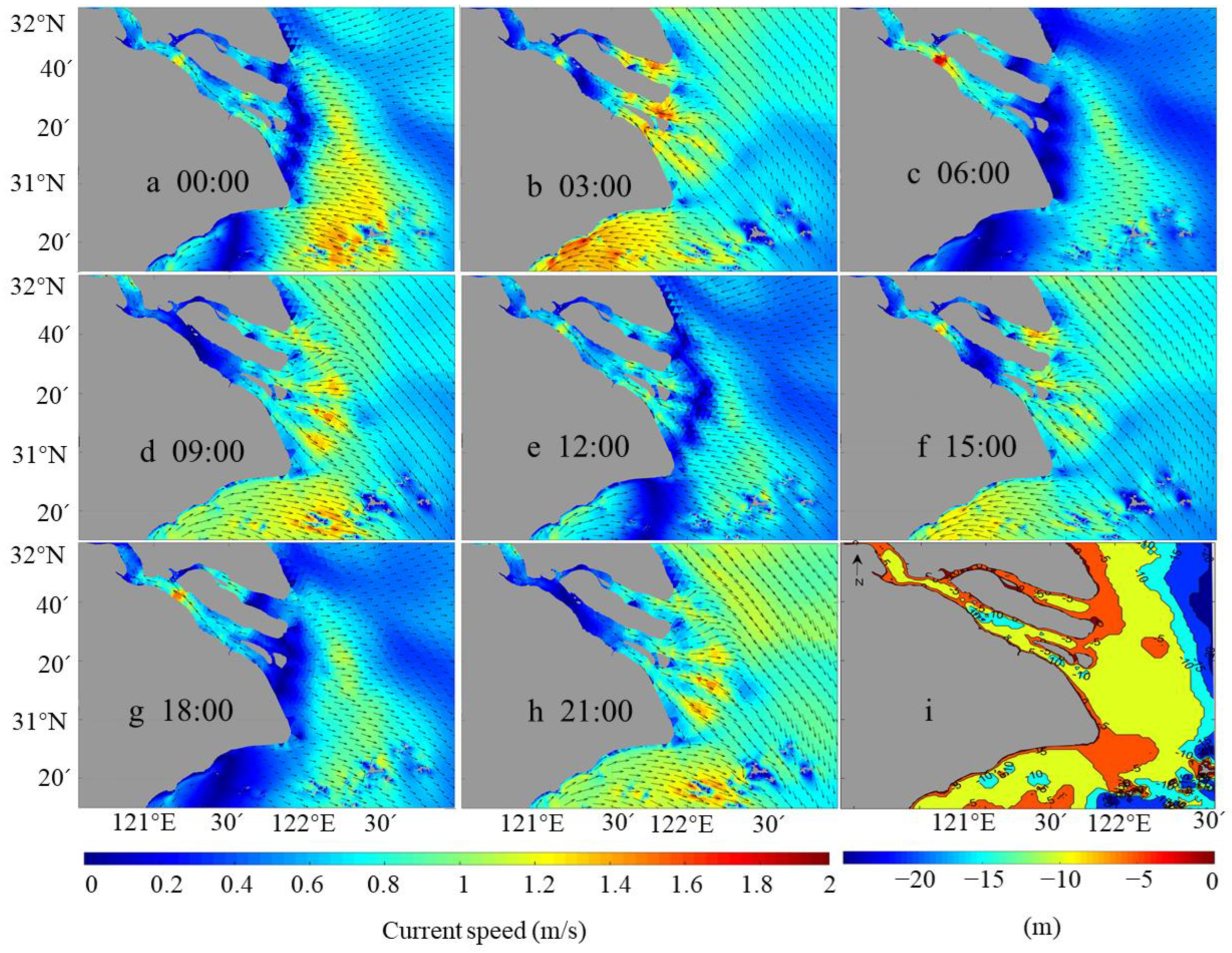
Diurnal variation and short-term changes of Chl-a concentration are closely related to the specific hydrodynamic conditions of the sea area (such as tide, resuspension, etc.) [8,9,10,69]. Tide in the Yangtze Mouth belongs to irregular semi-diurnal tide, and tide outside the mouth belongs to regular semi-diurnal tide [70]. The tidal current flows reciprocally inside the mouth, and gradually deforms into rotational current outside the mouth. During flood time, the high concentration area of Chl-a is distributed in the northwest mouth of Yangtze River as well as inside the Yangtze River; phytoplankton enters the water area of the station along with the water flow in the high-value area, and the Chl-a concentration peak is formed (Figure 5). During ebb tide, the high Chl-a concentration area shifted to the southeast as a whole. The shallow sea area outside the mouth of the Yangtze River is scoured by the tidal action and topographic jet action, and the tidal effect is obvious, which is a strong tidal area and rich in tidal energy resources. Tidal current impacts the distribution, and as tidal waves move, the distribution of Chl-a concentration on the surface of the sea changes (Figure 7) [28]. The asymmetrical duration of ebb and flow indicates that the duration of ebb and flow is shorter, which is conducive to the landward movement of fine sediment [66]. The asymmetry of the ebb and flow velocity indicates that the ebb and flow velocity is predominant in the Yangtze Mouth; both the velocity and duration of the ebb are larger than those of the flood (Figure 10), which is conducive to the movement of coarse sediment carrying nutrient substances to the sea [5,6,7,69].
In addition, due to the relatively shallow water depth (10 m) at the mouth and the consistent intense mixing of the water, the resuspended benthic microalgae and nutrients may make an important contribution to Chl-a concentration [71]. Suspended sediment (Figure 9) in Yangtze Mouth mainly comes from the Yangtze River; sediment from Subei Shoal and Qiantang River can also be brought into the Yangtze Mouth along with the flood current [72]. As the carrier of nutrients [73], suspended sediment will influence Chl-a by affecting phytoplankton and zooplankton [20] (Figure 5 and Figure 9). The uneven distribution patterns of water quality factors such as SSC (Figure 9) will ultimately influence the surrounding ecosystem of the estuary [36] (Figure 5, Figure 6 and Figure 7).
4.2.2. The Influence of Seasonal Related Factors on Chl-a
The variation of Chl-a concentration showed significant seasonal change. During flood season in summer (June to August), the runoff of the Yangtze River is very large, and the nearshore SSC is high, which carries many nutrients and is conducive to the growth of phytoplankton, inducing Chl-a to increase or decrease. In the dry season of winter, however, the runoff of the Yangtze River is small and the near-shore SSC becomes low; Chl-a concentration also decreases [74] and stays low [75]. In winter, many combined factors, including the disappearance of coastal upwelling, the enhancement of coastal current in the Yellow Sea, the enhancement of Taiwan warm current in the offshore area, and the southwardly diffused diluted water [37,76], can induce the decrease of surface SSC and the lower Chl-a concentration.
Lighting conditions also play an important role in the Chl-a concentration [77]. Phytoplankton adapts to the turbidity state by adjusting the light utilization efficiency [78]. The growth peak of phytoplankton under low light was slightly lower than that under high light in autumn (Figure 7) [77,79]. After the peak, the growth of phytoplankton was restricted under strong light, and Chl-a concentration showed a downward trend [80,81].
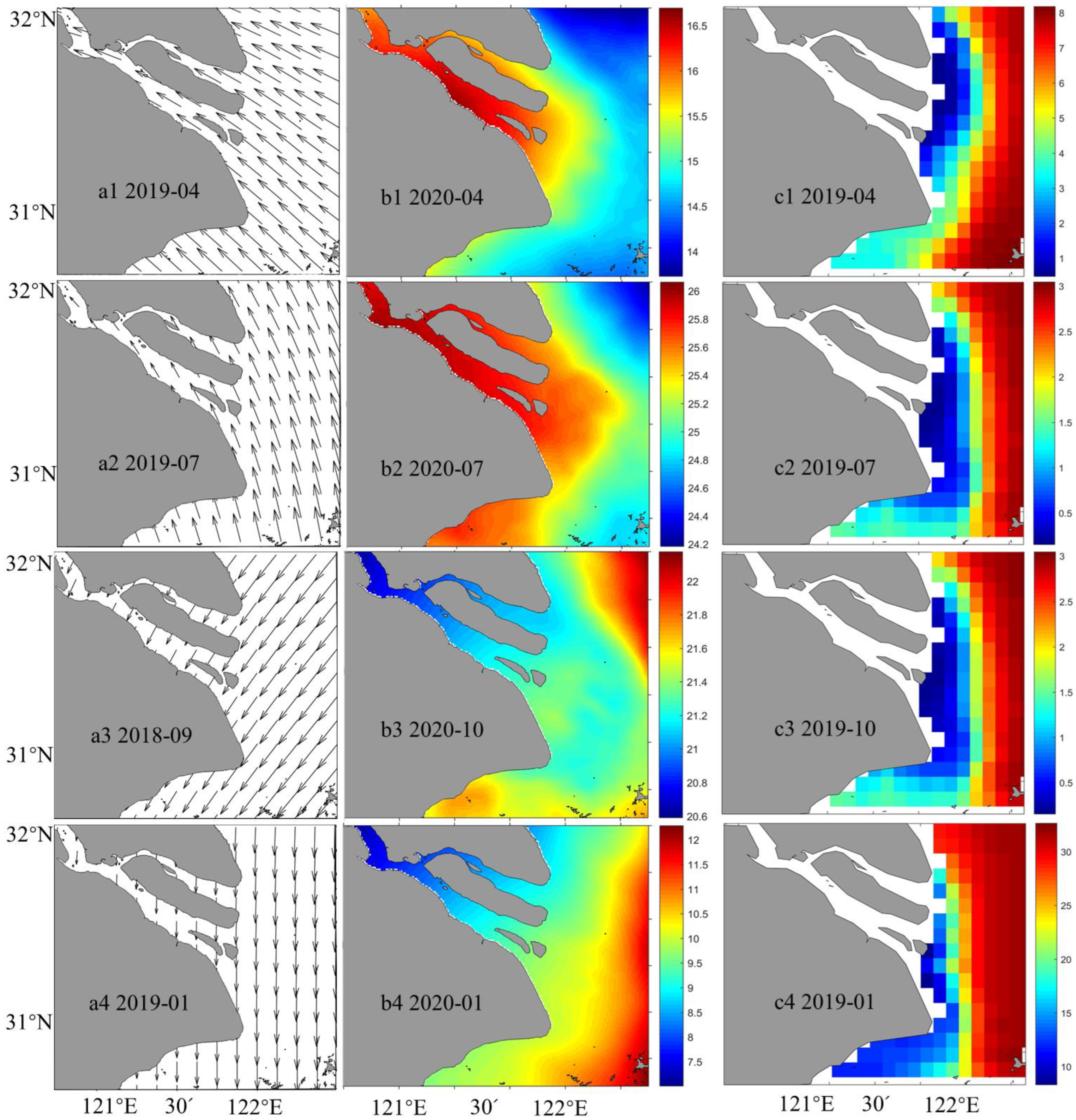
Monsoon, sea surface temperature (SST) [69], and sea surface salinity (SSS) [81] can also influence Chl-a concentration [67,77,81,82,83,84,85,86]. South and southeast monsoon dominates in spring and summer (Figure 11a1–a4). The southern wind is favorable for the formation of coastal upwelling [83], and the upwelling and cold vortex after strong winds are favorable for the growth of phytoplankton [84,85]. Wind-induced vorticity not only increases Chl-a distribution temporally but also spatially [19]. In addition, due to the increase of the Yangtze River runoff, the nutrient content in the area also increased, and the surface SSC increased, resulting in a high overall concentration of Chl-a (Figure 9). In autumn and winter, the northern wind controls the sea area (Figure 11a3,a4). Although convective mixing is strong and the depth of the mixing layer reaches the highest throughout the year, which makes the surface nutrients sufficient (Figure 11c3,c4), the growth of phytoplankton is severely restricted due to low temperature (Figure 11b3,b4) and insufficient sunshine.
5. Conclusions
The details of Chl-a concentration distribution and details of change in the Yangtze River Mouth were revealed based on a newly built Chl-a inversion model (PMS-C). Chl-a concentration in Yangtze River Mouth was in the range of 2–6 µg/L, being higher in the west than in the east. High Chl-a area was mainly distributed near the mouth of the Yangtze River and the Chl-a value was in the range of 3.7 µg/L to 5.9 µg/L. Chl-a concentration is higher in spring and summer than in autumn and winter, with a difference of 1–2 µg/L.
Short-term (within 3 h) changes of Chl-a concentration were effectively detected. In summer and autumn, Chl-a obtained at 13:30 at noon was generally lower than Chl-a obtained at around 10:30 in the morning and it decreased by nearly 0.1–4 μg/L within three hours in the same day. In winter, the concentration of Chl-a decreased in the range of 0–1.9 μg/L. Chl-a downstream of islands and bridges increased by 0.5–1.7 µg/L compared with upstream. Generally, downstream of islands and bridges, Chl-a reduced significantly to around 3.8 μg/L and 3 μg/L from the value of 5 μg/L and 3.7 μg/L in the morning, respectively. The current interacts with islands and piers, and vortex streets are induced downstream. The flow of vortex street makes the water exchange actively, increasing the suspended matter and nutrients, which leads to the increase of Chl-a concentration.
Environmental factors including seawater temperature, illumination, and nutrients, as well as dynamic factors such as wind and tidal current, can induce Chl-a change in the Yangtze River Mouth. Short-term change of Chl-a concentration is closely related to the specific hydrodynamic conditions, nutrients, and lighting conditions.
Author Contributions
J.B. conducted the research, data collecting, processing, analysis, and manuscript writing. L.C. conducted the research design, data collecting, processing, analysis, and manuscript writing. X.Y. conducted the data collecting and research advisement. H.X. and H.H. assisted in paper editing. J.J. assisted in data collecting. All authors have read and agreed to the published version of the manuscript.
Funding
This work is jointly supported by the following research projects: Zhejiang Key Science and Technology Project (2020C02004); National Natural Science Foundation of China Key international (regional) cooperative research project (42020104009); Basic Public Welfare Research Program of Zhejiang Province (LGF21D010004); Curriculum ideological and political teaching research project in the university of Zhejiang province (grouped ideological and political teaching model research in the subject of marine remote sensing).
Institutional Review Board Statement
Not applicable.
Informed Consent Statement
Not applicable.
Data Availability Statement
Not applicable.
Acknowledgments
GF-4 satellite data were obtained from the website: https://osdds.nsoas.org.cn accessed on 15 March 2021. The data product of HY-1C satellite was provided by National Satellite Ocean Application Service, MNR of PRC. The authors wish to thank the national satellite ocean application center, China and Sophisticated Ocean Front and Fisheries Investigation (SOPHI) for the data support.
Conflicts of Interest
The authors declare no conflict of interest.
References
- Yang, P.; Lai, D.Y.F.; Jin, B.; Bastviken, D.; Tan, L.; Tong, C. Dynamics of dissolved nutrients in the aquaculture shrimp ponds of the Min River estuary, China: Concentrations, fluxes and environmental loads. Sci. Total Environ. 2017, 603, 256–267. [Google Scholar] [CrossRef] [PubMed] [Green Version]
- Mo, Q.; Chen, N.; Zhou, X.; Chen, J.; Duan, S. Ammonium and phosphate enrichment across the dry-wet transition and their ecological relevance in a subtropical reservoir, China. Environ. Sci. Process. Impacts 2016, 18, 882–894. [Google Scholar] [CrossRef] [PubMed]
- Stringfellow, W.T.; Jain, R. Engineering the global ecosystem. Clean Technol. Environ. Policy 2010, 12, 197–203. [Google Scholar] [CrossRef] [Green Version]
- Watanabe, F.S.; Alcantara, E.; Rodrigues, T.W.; Imai, N.N.; Barbosa, C.C.; Rotta, L.H. Estimation of Chlorophyll-a Concentration and the Trophic State of the Barra Bonita Hydroelectric Reservoir Using OLI/Landsat-8 Images. Int. J. Environ. Res. Public Health 2015, 12, 10391–10417. [Google Scholar] [CrossRef] [PubMed]
- Cheng, L.; AghaKouchak, A.; Gilleland, E.; Katz, R.W. Non-stationary extreme value analysis in a changing climate. Clim. Chang. 2014, 127, 353–369. [Google Scholar] [CrossRef]
- Pei, S.; Shen, Z.; Laws, E.A. Nutrient Dynamics in the Upwelling Area of Changjiang (Yangtze River) Estuary. J. Coast. Res. 2009, 253, 569–580. [Google Scholar] [CrossRef]
- Wang, Y.; Jiang, H.; Jin, J.; Zhang, X.; Lu, X.; Wang, Y. Spatial-Temporal Variations of Chlorophyll-a in the Adjacent Sea Area of the Yangtze River Estuary Influenced by Yangtze River Discharge. Int. J. Environ. Res. Public Health 2015, 12, 5420–5438. [Google Scholar] [CrossRef] [Green Version]
- Liu, X.; Chen, Z.; Wu, J.; Cui, Z.; Su, P. Sedimentary polycyclic aromatic hydrocarbons (PAHs) along the mouth bar of the Yangtze River Estuary: Source, distribution, and potential toxicity. Mar. Pollut. Bull. 2020, 159, 111494. [Google Scholar] [CrossRef]
- Siegel, H.; Gerth, M.; Ohde, T.; Heene, T. Ocean colour remote sensing relevant water constituents and optical properties of the Baltic Sea. Int. J. Remote Sens. 2007, 26, 315–330. [Google Scholar] [CrossRef]
- Lei, H.; Bai, Y.; Huang, H.; Pan, D.; Mao, Z. Seasonal variation of absorption spectral characteristics of CDOM and de-pigmented particles in East China Sea. In Proceedings of the Remote Sensing of the Ocean, Sea Ice, and Large Water Regions, Cardiff, UK, 13 October 2008. [Google Scholar]
- Yu, X.; Xu, J.; Long, A.; Li, R.; Shi, Z.; Li, Q.P. Carbon-to-chlorophyll ratio and carbon content of phytoplankton community at the surface in coastal waters adjacent to the Zhujiang River Estuary during summer. Acta. Oceanol. Sin. 2020, 39, 123–131. [Google Scholar] [CrossRef]
- Lu, Z.; Liu, D.; Liao, J.; Wang, J.; Li, H.; Zhang, J. Characterizing spatial distribution of chlorophyll a in the Southern Ocean on a circumpolar cruise in summer. Sci. Total Environ. 2020, 708, 134833. [Google Scholar] [CrossRef] [PubMed]
- Papenfus, M.; Schaeffer, B.; Pollard, A.I.; Loftin, K. Exploring the potential value of satellite remote sensing to monitor chlorophyll-a for US lakes and reservoirs. Environ. Monit. Assess. 2020, 192, 808. [Google Scholar] [CrossRef] [PubMed]
- Kim, Y.H.; Son, S.; Kim, H.C.; Kim, B.; Park, Y.G.; Nam, J.; Ryu, J. Application of satellite remote sensing in monitoring dissolved oxygen variabilities: A case study for coastal waters in Korea. Environ. Int. 2020, 134, 105301. [Google Scholar] [CrossRef] [PubMed]
- Modiegi, M.; Rampedi, I.T.; Tesfamichael, S.G. Comparison of multi-source satellite data for quantifying water quality parameters in a mining environment. J. Hydrol. 2020, 591, 125322. [Google Scholar] [CrossRef]
- Reinart, A.; Kutser, T. Comparison of different satellite sensors in detecting cyanobacterial bloom events in the Baltic Sea. Remote Sens. Environ. 2006, 102, 74–85. [Google Scholar] [CrossRef]
- Liu, L.; Zhang, H.; Li, X.; Liu, C.; He, B.; Liu, K.; Zhang, X.; Li, M.; Yi, Y.; Lao, Y. Study on the quantitative model of suspended sediment from MODIS in the Yangtze River. In Proceedings of the Geoinformatics 2008 and Joint Conference on GIS and Built Environment: Monitoring and Assessment of Natural Resources and Environments, Guangzhou, China, 3 November 2008. [Google Scholar]
- Ahmed, W.; Wu, Y.; Kidwai, S.; Li, X.; Zhang, G.; Zhang, J. Spatial and temporal variations of nutrients and chlorophyll a in the Indus River and its deltaic creeks and coastal waters (Northwest Indian Ocean, Pakistan). J. Mar. Syst. 2021, 218, 103525. [Google Scholar] [CrossRef]
- Cai, L.; Bu, J.; Tang, D.; Zhou, M.; Yao, R.; Huang, S. Geosynchronous Satellite GF-4 Observations of Chlorophyll-a Distribution Details in the Bohai Sea, China. Sensors 2020, 20, 5471. [Google Scholar] [CrossRef]
- Yamaguchi, H.; Ishizaka, J.; Siswanto, E.; Baek Son, Y.; Yoo, S.; Kiyomoto, Y. Seasonal and spring interannual variations in satellite-observed chlorophyll-a in the Yellow and East China Seas: New datasets with reduced interference from high concentration of resuspended sediment. Cont. Shelf Res. 2013, 59, 1–9. [Google Scholar] [CrossRef] [Green Version]
- Garbulsky, M.F.; Filella, I.; Verger, A.; Peñuelas, J. Photosynthetic light use efficiency from satellite sensors: From global to Mediterranean vegetation. Environ. Exp. Bot. 2014, 103, 3–11. [Google Scholar] [CrossRef]
- Petus, C.; Waterhouse, J.; Lewis, S.; Vacher, M.; Tracey, D.; Devlin, M. A flood of information: Using Sentinel-3 water colour products to assure continuity in the monitoring of water quality trends in the Great Barrier Reef (Australia). J. Environ. Manag. 2019, 248, 109255. [Google Scholar] [CrossRef]
- Siswanto, E.; Tang, J.; Yamaguchi, H.; Ahn, Y.-H.; Ishizaka, J.; Yoo, S.; Kim, S.-W.; Kiyomoto, Y.; Yamada, K.; Chiang, C.; et al. Empirical ocean-color algorithms to retrieve chlorophyll-a, total suspended matter, and colored dissolved organic matter absorption coefficient in the Yellow and East China Seas. J. Oceanogr. 2011, 67, 627–650. [Google Scholar] [CrossRef]
- Wang, D. Remote Sensing-Based Study on the Temporal Variations in Chlorophyll-a Concentration After Confo Oil Spill in Bohai Sea. J. Indian Soc. Remote Sens. 2014, 43, 133–142. [Google Scholar] [CrossRef]
- Cui, T.; Zhang, J.; Tang, J.; Sathyendranath, S.; Groom, S.; Ma, Y.; Zhao, W.; Song, Q. Assessment of satellite ocean color products of MERIS, MODIS and SeaWiFS along the East China Coast (in the Yellow Sea and East China Sea). ISPRS J. Photogramm. Remote Sens. 2014, 87, 137–151. [Google Scholar] [CrossRef]
- Neumann, A.; Krawczyk, H.; Riha, S. Remote Sensing of Coastal Water Quality in the Baltic Sea Using MERIS. In Advances in Earth Observation of Global Change; Springer: Dordrecht, The Netherlands, 2010; pp. 55–67. [Google Scholar] [CrossRef]
- Cao, Z.; Ma, R.; Duan, H.; Xue, K. Effects of broad bandwidth on the remote sensing of inland waters: Implications for high spatial resolution satellite data applications. ISPRS J. Photogramm. Remote Sens. 2019, 153, 110–122. [Google Scholar] [CrossRef]
- He, C.; Yao, Y.; Lu, X.; Chen, M.; Ma, W.; Zhou, L. Exploring the Influence Mechanism of Meteorological Conditions on the Concentration of Suspended Solids and Chlorophyll-a in Large Estuaries Based on MODIS Imagery. Water 2019, 11, 375. [Google Scholar] [CrossRef] [Green Version]
- Wang, M.; Cheng, Y.; Chang, X.; Jin, S.; Zhu, Y. On-orbit geometric calibration and geometric quality assessment for the high-resolution geostationary optical satellite GaoFen4. ISPRS J. Photogramm. Remote Sens. 2017, 125, 63–77. [Google Scholar] [CrossRef]
- Wang, M.; Cheng, Y.; Tian, Y.; He, L.; Wang, Y. A New On-Orbit Geometric Self-Calibration Approach for the High-Resolution Geostationary Optical Satellite GaoFen4. IEEE J. Sel. Top. Appl. Earth Obs. Remote Sens. 2018, 11, 1670–1683. [Google Scholar] [CrossRef]
- Liu, Y.; Yao, L.; Xiong, W.; Zhou, Z. GF-4 Satellite and Automatic Identification System Data Fusion for Ship Tracking. IEEE Geosci. Remote Sens. Lett. 2019, 16, 281–285. [Google Scholar] [CrossRef]
- Li, F.; Xin, L.; Guo, Y.; Gao, D.; Kong, X.; Jia, X. Super-Resolution for GaoFen-4 Remote Sensing Images. IEEE Geosci. Remote Sens. Lett. 2018, 15, 28–32. [Google Scholar] [CrossRef]
- Ma, Z.; Wang, Y.; Gan, X.; Li, B.; Cai, Y.; Chen, J. Waterbird population changes in the wetlands at Chongming Dongtan in the Yangtze River estuary, China. Environ. Manag. 2009, 43, 1187–1200. [Google Scholar] [CrossRef]
- Wang, J.; Jin, P.; Bishop, P.L.; Li, F. Upgrade of three municipal wastewater treatment lagoons using a high surface area media. Front. Environ. Sci. Eng. 2011, 6, 288–293. [Google Scholar] [CrossRef]
- Cai, L.; Zhou, M.; Liu, J.; Tang, D.; Zuo, J. HY-1C Observations of the Impacts of Islands on Suspended Sediment Distribution in Zhoushan Coastal Waters, China. Remote Sens. 2020, 12, 1766. [Google Scholar] [CrossRef]
- Liu, X.; Chen, Z.; Xia, C.; Wu, J.; Ding, Y. Characteristics, distribution, source and ecological risk of polycyclic aromatic hydrocarbons (PAHs) in sediments along the Yangtze River Estuary Deepwater Channel. Mar. Pollut. Bull. 2020, 150, 110765. [Google Scholar] [CrossRef] [PubMed]
- Guo, X.; Fan, D.; Zheng, S.; Wang, H.; Zhao, B.; Qin, C. Revisited sediment budget with latest bathymetric data in the highly altered Yangtze (Changjiang) Estuary. Geomorphology 2021, 391, 107873. [Google Scholar] [CrossRef]
- Yang, A.; Zhong, B.; Wu, S.; Liu, Q. Radiometric Cross-Calibration of GF-4 in Multispectral Bands. Remote Sens. 2017, 9, 232. [Google Scholar] [CrossRef] [Green Version]
- Ghimire, P.; Lei, D.; Juan, N. Effect of Image Fusion on Vegetation Index Quality—A Comparative Study from Gaofen-1, Gaofen-2, Gaofen-4, Landsat-8 OLI and MODIS Imagery. Remote Sens. 2020, 12, 1550. [Google Scholar] [CrossRef]
- Xu, J.; Liang, Y.; Liu, J.; Huang, Z. Multi-Frame Super-Resolution of Gaofen-4 Remote Sensing Images. Sensors 2017, 17, 2142. [Google Scholar] [CrossRef] [Green Version]
- Ji, H.; Tian, L.; Li, J.; Tong, R.; Guo, Y.; Zeng, Q. Spatial–Spectral Fusion of HY-1C COCTS/CZI Data for Coastal Water Remote Sensing Using Deep Belief Network. IEEE J. Sel. Top. Appl. Earth Obs. Remote Sens. 2021, 14, 1693–1704. [Google Scholar] [CrossRef]
- Huang, S.; Liu, J.; Cai, L.; Zhou, M.; Bu, J.; Xu, J. Satellites HY-1C and Landsat 8 Combined to Observe the Influence of Bridge on Sea Surface Temperature and Suspended Sediment Concentration in Hangzhou Bay, China. Water 2020, 12, 2595. [Google Scholar] [CrossRef]
- Lan, S.; Wu, L.; Zhang, D.; Hu, C.; Liu, Y. Ethanol outperforms multiple solvents in the extraction of chlorophyll-a from biological soil crusts. Soil Biol. Biochem. 2011, 43, 857–861. [Google Scholar] [CrossRef]
- Wang, F.; Zhou, B.; Xu, J.; Song, L.; Wang, X. Application of neural network and MODIS 250m imagery for estimating suspended sediments concentration in Hangzhou Bay, China. Environ. Geol. 2008, 56, 1093–1101. [Google Scholar] [CrossRef]
- Muchsin, F.; Dirghayu, D.; Prasasti, I.; Rahayu, M.I.; Fibriawati, L.; Pradono, K.A.; Hendayani; Mahatmanto, B. Comparison of atmospheric correction models: FLAASH and 6S code and their impact on vegetation indices (case study: Paddy field in Subang District, West Java). IOP Conf. Ser. Earth Environ. Sci. 2019, 280, 012034. [Google Scholar] [CrossRef] [Green Version]
- Perkins, T. Speed and accuracy improvements in FLAASH atmospheric correction of hyperspectral imagery. Opt. Eng. 2012, 51, 111707. [Google Scholar] [CrossRef]
- Pan, G.; Wu, L.; Li, L.; Zhang, X.; Gong, W.; Wood, Y. Organic carbon stratification and size distribution of three typical paddy soils from Taihu Lake region, China. J. Environ. Sci. 2008, 20, 456–463. [Google Scholar] [CrossRef]
- Wang, T.; Zhang, G.; Yu, L.; Zhao, R.; Deng, M.; Xu, K. Multi-Mode GF-3 Satellite Image Geometric Accuracy Verification Using the RPC Model. Sensors 2017, 17, 2005. [Google Scholar] [CrossRef] [Green Version]
- Wens, V.; Marty, B.; Mary, A.; Bourguignon, M.; Op de Beeck, M.; Goldman, S.; Van Bogaert, P.; Peigneux, P.; De Tiege, X. A geometric correction scheme for spatial leakage effects in MEG/EEG seed-based functional connectivity mapping. Hum. Brain Mapp. 2015, 36, 4604–4621. [Google Scholar] [CrossRef] [PubMed]
- Dubey, B.; Kartikeyan, B.; Subbiah, M.M. Rational Polynomial Coefficients Modeling and Bias Correction by Using Iterative Polynomial Augmentation. J. Indian Soc. Remote Sens. 2018, 47, 165–175. [Google Scholar] [CrossRef]
- Gu, Y.; Brown, J.F.; Verdin, J.P.; Wardlow, B. A five-year analysis of MODIS NDVI and NDWI for grassland drought assessment over the central Great Plains of the United States. Geophys. Res. Lett. 2007, 34, 1–6. [Google Scholar] [CrossRef] [Green Version]
- Eid, A.N.M.; Olatubara, C.O.; Ewemoje, T.A.; El-Hennawy, M.T.; Farouk, H. Inland wetland time-series digital change detection based on SAVI and NDWI indecies: Wadi El-Rayan lakes, Egypt. Remote Sens. Appl. Soc. Environ. 2020, 19, 100347. [Google Scholar] [CrossRef]
- Chen, C.; Beardsley, R.C.; Cowles, G. An Unstructured Grid, Finite-Volume Coastal Ocean Model: FVCOM User Manual, 2nd ed.; Massachusetts Institute of Technology: Cambridge, MA, USA, 2012. [Google Scholar]
- Chen, C.; Liu, H.; Beardsley, R.C. An unstructured, finite-volume, three-dimensional, primitive equation ocean model: Application to coastal ocean and estuaries. J. Atmos. Ocea. Estuaries 2003, 20, 159–186. [Google Scholar] [CrossRef]
- Yang, Z.; Shao, W.; Ding, Y.; Shi, J.; Ji, Q. Wave Simulation by the SWAN Model and FVCOM Considering the Sea-Water Level around the Zhoushan Islands. J. Mar. Sci. Eng. 2020, 8, 783. [Google Scholar] [CrossRef]
- Xue, P.; Chen, C.; Ding, P.; Beardsley, R.C.; Lin, H.; Ge, J.; Kong, Y. Saltwater intrusion into the Changjiang River: A model-guided mechanism study. J. Geophys. Res. Ocean. 2009, 114, 1–15. [Google Scholar] [CrossRef]
- Chen, C.; Qi, J.; Li, C.; Beardsley, R.C.; Lin, H.; Walker, R.; Gates, K. Complexity of the flooding/drying process in an estuarine tidal-creek salt-marsh system: An application of FVCOM. J. Geophys. Res. Ocean. 2008, 113, 1–21. [Google Scholar] [CrossRef] [Green Version]
- Josey, S.A.; Kent, E.C.; Taylor, P.K. Wind stress forcing of the ocean in the SOC climatology: Comparisons with the NCEP-NCAR, ECMWF, UWM/COADS, and Hellerman and Rosenstein datasets. J. Phys. Oceanogr. 2002, 32, 1993–2019. [Google Scholar] [CrossRef]
- Bormann, N.; Fouilloux, A.; Bell, W. Evaluation and assimilation of ATMS data in the ECMWF system. J. Geophys. Res. Atmos. 2013, 118, 12970–12980. [Google Scholar] [CrossRef]
- Lawrence, H.; Bormann, N.; Geer, A.J.; Lu, Q.; English, S.J. Evaluation and Assimilation of the Microwave Sounder MWHS-2 Onboard FY-3C in the ECMWF Numerical Weather Prediction System. IEEE Trans. Geosci. Remote Sens. 2018, 56, 3333–3349. [Google Scholar] [CrossRef]
- Chassignet, E.P.; Hurlburt, H.E.; Smedstad, O.M.; Halliwell, G.R.; Hogan, P.J.; Wallcraft, A.J.; Baraille, R.; Bleck, R. The HYCOM (HYbrid Coordinate Ocean Model) data assimilative system. J. Mar. Syst. 2007, 65, 60–83. [Google Scholar] [CrossRef]
- Halliwell, G.R. Evaluation of vertical coordinate and vertical mixing algorithms in the HYbrid-Coordinate Ocean Model (HYCOM). Ocean Model. 2004, 7, 285–322. [Google Scholar] [CrossRef]
- Drake, J.L.; Carpenter, E.J.; Cousins, M.; Nelson, K.L.; Guido-Zarate, A.; Loftin, K. Effects of light and nutrients on seasonal phytoplankton succession in a temperate eutrophic coastal lagoon. Hydrobiologia 2010, 654, 177–192. [Google Scholar] [CrossRef] [Green Version]
- Feng, W.; Zhu, Q.; Zhuang, J.; Yu, S. An expert recommendation algorithm based on Pearson correlation coefficient and FP-growth. Clust. Comput. 2018, 22, 7401–7412. [Google Scholar] [CrossRef]
- Heo, J.-H.; Kho, Y.W.; Shin, H.; Kim, S.; Kim, T. Regression equations of probability plot correlation coefficient test statistics from several probability distributions. J. Hydrol. 2008, 355, 1–15. [Google Scholar] [CrossRef]
- Wang, Y.; Xu, H.; Li, M. Long-term changes in phytoplankton communities in China’s Yangtze Estuary driven by altered riverine fluxes and rising sea surface temperature. Geomorphology 2021, 376, 107566. [Google Scholar] [CrossRef]
- Li, Y.; Chen, B.-M.; Wang, Z.-G.; Peng, S.-L. Effects of temperature change on water discharge, and sediment and nutrient loading in the lower Pearl River basin based on SWAT modelling. Hydrol. Sci. J. 2011, 56, 68–83. [Google Scholar] [CrossRef] [Green Version]
- Zhang, L.-L.; Li, H.-X. Weighted Pseudo-Almost Periodic Solutions for Some Abstract Differential Equations with Uniform Continuity. Bull. Aust. Math. Soc. 2010, 82, 424–436. [Google Scholar] [CrossRef] [Green Version]
- Ge, J.; Torres, R.; Chen, C.; Liu, J.; Xu, Y.; Bellerby, R.; Shen, F.; Bruggeman, J.; Ding, P. Influence of suspended sediment front on nutrients and phytoplankton dynamics off the Changjiang Estuary: A FVCOM-ERSEM coupled model experiment. J. Mar. Syst. 2020, 204, 103292. [Google Scholar] [CrossRef]
- Hou, L.J.; Liu, M.; Xu, S.Y.; Ou, D.N.; Lu, J.J.; Yu, J.; Cheng, S.B.; Yang, Y. The effects of semi-lunar spring and neap tidal change on nutrients cycling in the intertidal sediments of the Yangtze estuary. Environ. Geol. 2005, 48, 255–264. [Google Scholar] [CrossRef]
- Kim, H.-S.; Hwang, S.-J.; Shin, J.-K.; An, K.-G.; Yoon, C.G. Effects of limiting nutrients and N:P ratios on the phytoplankton growth in a shallow hypertrophic reservoir. Hydrobiologia 2007, 581, 255–267. [Google Scholar] [CrossRef]
- Dai, Z.; Fagherazzi, S.; Mei, X.; Gao, J. Decline in suspended sediment concentration delivered by the Changjiang (Yangtze) River into the East China Sea between 1956 and 2013. Geomorphology 2016, 268, 123–132. [Google Scholar] [CrossRef] [Green Version]
- Zhuang, W.; Zhou, F. Distribution, source and pollution assessment of heavy metals in the surface sediments of the Yangtze River Estuary and its adjacent East China Sea. Mar. Pollut. Bull. 2021, 164, 112002. [Google Scholar] [CrossRef]
- Jiang, Z.; Liu, J.; Chen, J.; Chen, Q.; Yan, X.; Xuan, J.; Zeng, J. Responses of summer phytoplankton community to drastic environmental changes in the Changjiang (Yangtze River) estuary during the past 50 years. Water Res 2014, 54, 1–11. [Google Scholar] [CrossRef]
- Oliver, R.L.; Mitrovic, S.M.; Rees, C. Influence of salinity on light conditions and phytoplankton growth in a turbid river. River Res. Appl. 2010, 26, 894–903. [Google Scholar] [CrossRef]
- Zhang, E.; Gao, S.; Savenije, H.H.G.; Si, C.; Cao, S. Saline water intrusion in relation to strong winds during winter cold outbreaks: North Branch of the Yangtze Estuary. J. Hydrol. 2019, 574, 1099–1109. [Google Scholar] [CrossRef]
- Sato, Y.; Bourne, D.G.; Willis, B.L. Effects of temperature and light on the progression of black band disease on the reef coral, Montipora hispida. Coral Reefs 2011, 30, 753–761. [Google Scholar] [CrossRef]
- Huang, W.; Han, S.; Zhou, Q.; Li, W.; Xing, W. Assessing interactions between environmental factors and aquatic toxicity: Influences of dissolved CO2 and light on Cd toxicity in the aquatic macrophyte Potamogeton crispus. Aquat. Toxicol. 2019, 212, 247–258. [Google Scholar] [CrossRef]
- Pepin, P.; Johnson, C.L.; Harvey, M.; Casault, B.; Chassé, J.; Colbourne, E.B.; Galbraith, P.S.; Hebert, D.; Lazin, G.; Maillet, G.; et al. A multivariate evaluation of environmental effects on zooplankton community structure in the western North Atlantic. Prog. Oceanogr. 2015, 134, 197–220. [Google Scholar] [CrossRef]
- Poulin, C.; Bruyant, F.; Laprise, M.-H.; Cockshutt, A.M.; Marie-Rose Vandenhecke, J.; Huot, Y. The impact of light pollution on diel changes in the photophysiology of Microcystis aeruginosa. J. Plankton Res. 2014, 36, 286–291. [Google Scholar] [CrossRef] [Green Version]
- Lashaway, A.R.; Carrick, H.J. Effects of light, temperature and habitat quality on meroplanktonic diatom rejuvenation in Lake Erie: Implications for seasonal hypoxia. J. Plankton Res. 2010, 32, 479–490. [Google Scholar] [CrossRef] [Green Version]
- Radchenko, I.G.; Ilyash, L.V.; Shevchenko, V.P.; Zdorovennov, R.E.; Novigatsky, A.N.; Politova, N.V.; Tolstikov, A.V. Spatial Distribution of Phytoplankton in the Subarctic Estuary (Kem’ River, the White Sea). Oceanology 2019, 59, 305–315. [Google Scholar] [CrossRef]
- Ma, J.; Liu, H.; Zhan, H.; Lin, P.; Du, Y. Effects of chlorophyll on upper ocean temperature and circulation in the upwelling regions of the South China Sea. Aquat. Ecosyst. Health Manag. 2012, 15, 127–134. [Google Scholar] [CrossRef]
- Huang, X.; Jing, Z.; Zheng, R.; Cao, H. Dynamical analysis of submesoscale fronts associated with wind-forced offshore jet in the western South China Sea. Acta Oceanol. Sin. 2021, 39, 1–12. [Google Scholar] [CrossRef]
- Yin, K.; Zhang, J.; Qian, P.-Y.; Jian, W.; Huang, L.; Chen, J.; Wu, M.C.S. Effect of wind events on phytoplankton blooms in the Pearl River estuary during summer. Cont. Shelf Res. 2004, 24, 1909–1923. [Google Scholar] [CrossRef]
- Schagerström, E.; Salo, T. Interactive effects of temperature and light on reattachment success in the brown alga Fucus radicans. Bot. Mar. 2019, 62, 43–50. [Google Scholar] [CrossRef] [Green Version]
Figure 1.
(a) Location of Yangtze River. (b) Blue square: study area.

Figure 2.
Correlation between the band value retrieved from PMS image after atmosphere correction and sampled Chl-a. (a) B2 (blue band); (b) B3 (green band); (c) B4 (red band); (d) B5 (NIR band).
Figure 2.
Correlation between the band value retrieved from PMS image after atmosphere correction and sampled Chl-a. (a) B2 (blue band); (b) B3 (green band); (c) B4 (red band); (d) B5 (NIR band).

Figure 3.
Correlation analysis between simulated and in situ Chl-a values.

Figure 4.
The distribution of Chl-a retrieved from PMS in the Yangtze River Mouth. (a–l): satellite images of different date. Black arrow: local current direction.
Figure 4.
The distribution of Chl-a retrieved from PMS in the Yangtze River Mouth. (a–l): satellite images of different date. Black arrow: local current direction.

Figure 5.
(a1–c1): Chl-a concentration retrieved from GF-4. Colored squares: Chl-a concentration distribution in the area near islands and bridge; (a2–c2): the red squares; (a3–c3): the blue squares; u: upstream; d: downstream.
Figure 5.
(a1–c1): Chl-a concentration retrieved from GF-4. Colored squares: Chl-a concentration distribution in the area near islands and bridge; (a2–c2): the red squares; (a3–c3): the blue squares; u: upstream; d: downstream.

Figure 6.
The distribution of Chl-a retrieved from Landsat 8-OLI in the Yangtze River Mouth. (a–f): satellite images of different date. Black arrow: local current direction.
Figure 6.
The distribution of Chl-a retrieved from Landsat 8-OLI in the Yangtze River Mouth. (a–f): satellite images of different date. Black arrow: local current direction.

Figure 7.
(a1–i1), (a2–i2), (a3–i3): Chl-a change in the same day (a4–i4): the decrease area of Chl-a. (a5–i5): The increase area of Chl-a.
Figure 7.
(a1–i1), (a2–i2), (a3–i3): Chl-a change in the same day (a4–i4): the decrease area of Chl-a. (a5–i5): The increase area of Chl-a.

Figure 8.
(a1–c1), (a2–c2), (a3–c3), (a4–c4), (a5–c5): Chl-a and its change at two different times of the day. (a4): (a2) minus (a1); (a5): (a3) minus (a2); (b4): (b2) minus (b1); (b5): (b3) minus (b2); (c4): (c2) minus (c1); (c5): (c3) minus (c2). Black ellipse: area of Chl-a concentration change.
Figure 8.
(a1–c1), (a2–c2), (a3–c3), (a4–c4), (a5–c5): Chl-a and its change at two different times of the day. (a4): (a2) minus (a1); (a5): (a3) minus (a2); (b4): (b2) minus (b1); (b5): (b3) minus (b2); (c4): (c2) minus (c1); (c5): (c3) minus (c2). Black ellipse: area of Chl-a concentration change.

Figure 9.
SSC distribution obtained from CZI image. (a–d): satellite images of different date. (a1–d1): Chl-a change upstream and downstream of island and project; u: upstream; d: downstream.
Figure 9.
SSC distribution obtained from CZI image. (a–d): satellite images of different date. (a1–d1): Chl-a change upstream and downstream of island and project; u: upstream; d: downstream.

Figure 10.
(a–h): Tidal current obtained every 3 h from 0:00 on 30 November 2020. (i): The bathymetric topographic map. Black arrow: tidal current direction.
Figure 10.
(a–h): Tidal current obtained every 3 h from 0:00 on 30 November 2020. (i): The bathymetric topographic map. Black arrow: tidal current direction.

Figure 11.
(a1–a4): Monthly wind field. (b1–b4): Monthly mean SST. (c1–c4): Monthly mean SSS.


Table 1.
Information for the GF-4 of sensors.
| Information | Panchromatic and Near-Infrared Sensor (nm) | Intermediate Infrared Sensor (nm) |
|---|---|---|
| Spectral range | B1: 450–900 | B6: 3500–4100 |
| B2: 450–520 | ||
| B3: 520–600 | ||
| B4: 630–690 | ||
| B5: 760–900 | ||
| Ground sample distance | 50 m | 400 m |
Table 2.
The parameters of CZI sensor and information about the images.
| Band | Wavelength (nm) | Spatial Resolution (m) | The Application Object |
|---|---|---|---|
| B1-Blue | 421–500 | 50 | Chlorophyll, pollution, ice, underwater terrain |
| B2-Green | 517–598 | Chlorophyll, medium and low concentration of sediment vegetation, ice, beach | |
| B3-Red | 608–690 | Suspended sediment, vegetation, soil | |
| B4-NIR | 761–891 | Vegetation, high concentration of sediment, atmospheric correction |
Table 3.
Eight retrieved formulas of Chl-a of PMS.
| Number | Band Combination (x) | Regression Equation (y = Chl-a) | Coefficient of Determination (R2) |
|---|---|---|---|
| 1 | ln(B3)/ln(B4) | y = 740.16x2 − 1537.9x + 801.2 | 0.8915 |
| 2 | ln(B3/B4) | y = 18.562x2 − 8.8034x + 3.4315 | 0.9044 |
| 3 | B3/(B3 + B4) | y = 306.27x2 − 341.85x + 97.779 | 0.9061 |
| 4 | (B3 + B2)/(B2 + B4) | y = 47.446x2 − 108.9x + 64.916 | 0.89 |
| 5 | (B4 + B2)/(B3 + B2) | y = 66.27x2 − 117.79x + 54.849 | 0.908 |
| 6 | (B3 − B4)/(B2 + B3) ★ | y = 66.27x2 − 14.751x + 3.3302 ★ | 0.9087 ★ |
| 7 | (B3 − B4)/(B2 + B4) | y = 47.446x2 − 14.007x + 3.4626 | 0.89 |
| 8 | (B3 − B4)/(B3 + B4) | y = 76.567x2 − 17.788x + 3.4236 | 0.9061 |
Publisher’s Note: MDPI stays neutral with regard to jurisdictional claims in published maps and institutional affiliations. |
© 2022 by the authors. Licensee MDPI, Basel, Switzerland. This article is an open access article distributed under the terms and conditions of the Creative Commons Attribution (CC BY) license (https://creativecommons.org/licenses/by/4.0/).
Share and Cite
MDPI and ACS Style
Bu, J.; Cai, L.; Yan, X.; Xu, H.; Hu, H.; Jiang, J. Monitoring the Chl-a Distribution Details in the Yangtze River Mouth Using Satellite Remote Sensing. Water 2022, 14, 1295. https://doi.org/10.3390/w14081295
AMA Style
Bu J, Cai L, Yan X, Xu H, Hu H, Jiang J. Monitoring the Chl-a Distribution Details in the Yangtze River Mouth Using Satellite Remote Sensing. Water. 2022; 14(8):1295. https://doi.org/10.3390/w14081295
Chicago/Turabian StyleBu, Juan, Lina Cai, Xiaojun Yan, Huanzhi Xu, Haiyan Hu, and Jingjing Jiang. 2022. "Monitoring the Chl-a Distribution Details in the Yangtze River Mouth Using Satellite Remote Sensing" Water 14, no. 8: 1295. https://doi.org/10.3390/w14081295
Note that from the first issue of 2016, this journal uses article numbers instead of page numbers. See further details here.