Short-Term Bathwater Demand Forecasting for Shared Shower Rooms in Smart Campuses Using Machine Learning Methods

Abstract

Water scarcity is a growing threat to humankind. At university campuses, there is a need for shared shower room managers to forecast the demand for bath water accurately. Accurate bath water demand forecasts can decrease the costs of water heating and pumping, reduce overall energy consumption, and improve student satisfaction (due to stability of bath water supply and bathwater temperature). We present a case study conducted at Capital Normal University (Beijing, China), which provides shared shower rooms separately for female and male students. Bath water consumption data are collected in real-time through shower tap controllers to forecast short-term bath water consumption in the shower buildings. We forecasted and compared daily and hourly bath water demand using the autoregressive integrated moving average, random forests, long short-term memory, and neural basis expansion analysis time series-forecasting models, and assessed the models’ performance using the mean absolute error, mean absolute percentage error, root-mean-square error, and coefficient of determination equations. Subsequently, covariates such as weather information, student behavior, and calendars were used to improve the models’ performance. These models achieved highly accurate forecasting for all the shower room areas. The results imply that machine learning methods outperform statistical methods (particularly for larger datasets) and can be employed to make accurate bath water demand forecasts.

1. Introduction

Water demand forecasting is an important issue in the field of water management worldwide [1]. Water scarcity is a growing threat to humankind and researchers have made many efforts, proposing solutions such as water treatment [2,3], water desalination [4], and optimization of water management systems [5] to compensate for the scarcity. Showers are common water consumption behaviors. In China, university students often take showers in shared shower rooms and pay water fees using their campus cards. It is necessary for shared shower room managers to forecast the bath water demand (BWD) using parameters such as the day of the week, hours of opening, weather, and holidays. Therefore, short-term BWD forecasting is key for efficient campus water management systems. Good operational and strategic decisions can help improve water distribution performance [3,6]; however, traditional time-series forecasting methods highlight the role of time without considering the effects of external factors, including meteorological factors, such as temperature, wind, and precipitation, and socioeconomic factors, such as population characteristics. Using machine learning (ML) to extract useful information from data provided by smart campuses, smart cities, retail, and industrial industries has recently gained popularity [7,8,9]. Businesses use ML to simplify mundane tasks, gain a competitive edge in the market, and increase earnings. The smart campus is a developed and competitive campus environment that integrates work, study, and living. It is built on the Internet of Things (IoT) [10]. Smart campuses have embraced the IoT to automate numerous scenarios, and the data created by these devices is uploaded (reported) to a cloud server for flow management and data analysis over the Internet [11,12].

In this study, our analysis was based on data collected from the shared shower rooms of Capital Normal University (CNU), Beijing, China. Similarly to many campuses in North China, the use of shared shower rooms open to students is more frequent in the afternoons and evenings (especially 3:00–10:00 p.m.) at CNU. Therefore, we selected autoregressive integrated moving average (ARIMA), ARIMA with exogenous input (ARIMAX), random forests (RF), long short-term memory (LSTM), and neural basis expansion analysis for interpretable time series forecasting (N-BEATS) to build short-term BWD forecasting models and applied these to shower buildings at CNU. Furthermore, we investigated the performance of demand forecasting in female and male shower areas. To the best of our knowledge, this is the first empirical study to use a forecasting technique to develop and evaluate the performance of machine learning techniques for the forecasting of BWD in shared shower rooms, considering the majority of articles [13,14,15] that conduct similar analyses often refer to total water demand. In addition, our findings in this study imply that there is a potential for energy savings and the decision making for bath water management may be used to promote energy savings in the future based on accurate BWD forecasts.

2. Literature Review

Accurate water demand forecasting helps ensure the security, stability, and economic operation of smart campuses. It is also advantageous in planning reasonable maintenance arrangements. Many factors can directly or indirectly influence BWD, including the variables of weather such as rainfall, temperature, and air quality, as well as other factors such as class schedules, weekends, and national holidays. Climate variables, in particular, have been frequently used as inputs to multivariate statistical models and machine learning approaches for modeling and predicting urban water time series [16,17,18,19].

According to Koo et al. [20], there are no universal methods for water demand forecasting, and forecasting time periods can be categorized as short term (minutes, hourly, daily, or weekly) [20,21], medium term (yearly, up to 24 months) [22], or long term (2-years, 10-years) [23,24]. Short-term BWD forecasting is beneficial for operational and managerial decision making, which can decrease overall energy consumption and increase the bath water quality (especially temperature). ML techniques such as LSTM [25], support vector machine [26] and random forest [21] have been widely employed to forecast short-term urban water demand. Accurate and dependable BWD forecasting is critical for bath water management systems and will aid in numerous elements of short-term planning and decision making (e.g., the planning of water boiling and pumping). This requires an accurate and dependable mechanism for BWD forecasting.

Forecasting water demand is a burgeoning subject of research. Numerous researchers have used both traditional statistical models and machine learning approaches to forecast water demand. In recent years, increasingly advanced ML techniques and toolkits have been created to address forecasting issues [27]. In the 2000s, shared showers in universities in North China began to automate their bath water supply using bath water management systems. The control logic of the early bath water management systems was rather simple: they recorded the time of shower room attendance but did not limit bath water consumption, resulting in inefficient energy and water resource consumption. However, the recent approaches employed by universities, such as IoT devices and smart campus cards [11], are more accurate and smarter in controlling shower behaviors. Thus, with the accumulation of bath water consumption data, the operation of the system can be optimized using forecasting techniques. Usually, the operators of shared shower rooms make BWD forecasts for the next day based on their experience and plan bath water boiling and flow control actions accordingly, which has always failed to make accurate forecasts. Accurate short-term BWD forecasting can help to minimize heating and pumping costs while also increasing consumer satisfaction. Numerous studies have suggested forecasting short-term water demand using classic statistics, machine learning, and deep neural network (DNN) models.

Linear models were among the first to be widely employed in forecasting water demand. According to Do et al. [28], an online demand multiplier particle filter can be used to forecast real-time water demand. The ARIMA model was used by Kofinas et al. [29] to forecast water demand in cities, with good performance forecasting the monthly average urban water demand. Wong et al. [30] forecasted Hong Kong’s daily water consumption using a correlation analysis of meteorological data and calendar impacts. For water demand forecasting, Hutton and Kapelan [31] found that using the repeated Bayesian likelihood model improved forecasting accuracy. Quevedo et al. [32] assessed the effects of seasonal ARIMA (SARIMA) and exponential smoothing models that took calendar effects into account and showed that they were superior in forecasting water demand when temporal and daily periods were considered. Furthermore, Patcha et al. [33] demonstrated that the ARIMAX model with dew point depression and average temperature input plays an important role in forecasting long-term water consumption rates in Las Vegas.

Candelieri et al. [34] applied a support vector machine (SVM) to forecast water demand and achieved high generalization ability and efficiency. Brentan et al. [35] forecasted water demand using a mix of SVM and adaptive Fourier series and obtained better results than SVM alone. Moreover, ML models, RF models [36], and extreme learning machine models [37] were seen to be more beneficial than statistical models.

However, studies demonstrate that linear regression methods, when compared to nonlinear regression models, have certain shortcomings in water demand forecasting due to the complexity and nonlinear realities of water demand [32,37,38]. Recent research has showed a strong interest in using neural network models to solve time series forecasting challenges. Neural networks are composed of many layers of computing units (neurons) that are connected by connections between the neurons in a layer [39]. A neuron in a network transforms data by performing the following computations: multiplying an initial value by a weight, adding the result to additional input values, adjusting the resulting number for the neuron’s bias, and lastly normalizing the output using an activation function [40]. After all connections are examined, the bias is a neuron-specific number that has an impact on the neuron’s value, and the activation function ensures that values are passed on within a configurable, predicted range. This procedure is repeated until the final output layer is capable of providing regression scores or predictions. All neurons in a particular layer provide an output; their weights are not identical to those in the following neuron layer. This implies that if a neuron on a layer detects a certain pattern, the whole image may suffer and the neuron may be partially or fully muted. A large weight indicates that the input is significant, whereas a lower weight indicates that it should be ignored. As a result, neural networks should be treated as complex systems that reveal complex behavior; rather than the neurons themselves, it is the interactions between the neurons that enable the network to learn.

To develop short-term forecasts of water consumption, Vijai et al. [41] evaluated DNN models with machine-learning techniques. Xenochristou et al. [42] compared forecasts of daily water consumption using a stacked model and a DNN model. Koo et al. [20] analyzed the performance evaluations of LSTM and ARIMA with those of ML models for distinguishing water usage in Korea, and found that the former performed better. In their study, Kuehnert et al. [25] explored the usefulness of LSTM models for water demand forecasting and showed that LSTM models outperformed the system in operation by a large margin. The cutting-edge N-BEATS model has demonstrated outstanding performance on large-scale time-series challenges. Boris et al. [22], for example, utilized N-BEATS to forecast mid-term electrical usage and showed that it outperformed statistical and machine learning approaches.

Previous studies [15,29,43,44,45,46,47,48] on water demand forecasting have mainly focused on total water consumption in urban or residential areas, given that a high proportion of bath water is hot water, and conservation of bath water has energy and greenhouse gas conservation benefits [49]. While several researchers have addressed and built water demand forecasting models, there is a dearth of study on the performance evaluation of short-term BWD forecasting in shared shower rooms.

3. Materials and Methods

At CNU, during the summer vacation of 2017, the shared shower rooms were equipped with smart shower taps controllable by IoT devices.

3.1. Study Process

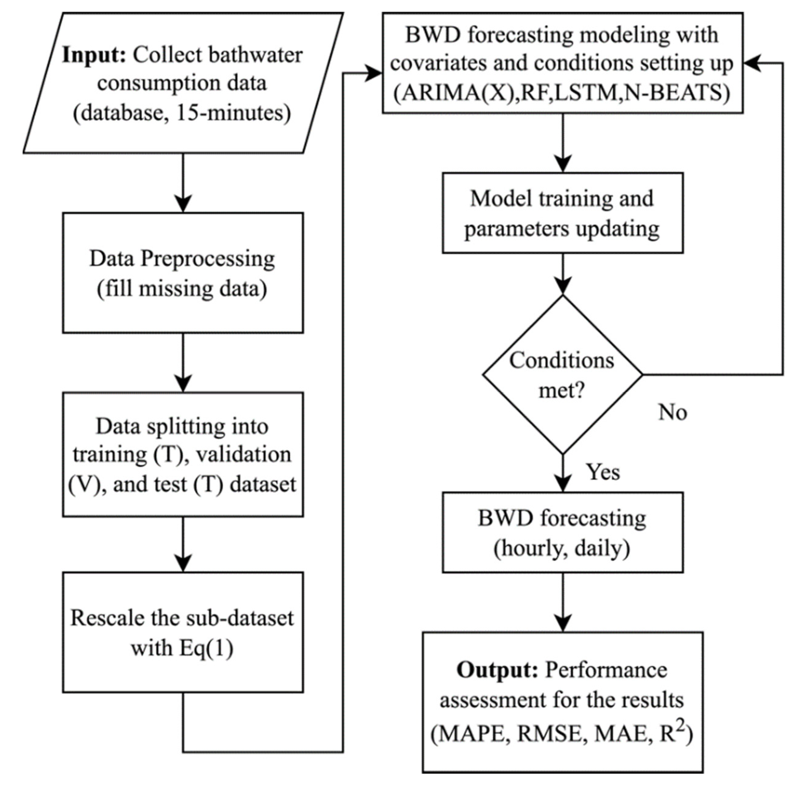
Three steps have been used in evaluating a short-term BWD-forecasting model: (a) model inputs were derived from pre-processed data obtained from CNU shower rooms; (b) to suit the real-world management requirements, daily and hourly scale forecasts of BWD were conducted. Because the data were collected via students’ shower bill history, bath water usage data were pre-processed by resampling on the target scale; and (c) forecasts were made using ARIMA, ARIMAX, RF, LSTM, and N-BEATS. The procedure is illustrated in Figure 1.

To model and evaluate BWD, the bath water consumption dataset was subdivided into training, validation, and test subsets. Generally, for the daily BWD forecast purpose, the test dataset contained points of the last 30 days, the training dataset contained points of 852 days (80% of the dataset) and validation datasets contained points of 213 days (20% of the dataset); for the purpose of hourly BWD forecasting, the test dataset contained the 35 points of the last 5 days (shared shower rooms serve 7 h per day), the training dataset contained 4352 points (80% of the dataset) and validation datasets contained 1088 points (20% of the dataset). In addition, for the LSTM and N-BEATS models, the data were scaled to minimize the forecasting bias introduced by Equation (1). The parameters of each forecasting model were estimated using the training and validation datasets. When the estimated parameters met the simulation constraints, the validation dataset was used to forecast the BWD for the following time step. To evaluate performance, we generated the mean absolute percentage error (MAPE), mean absolute error (MAE), root-mean-square error (RMSE), and coefficient of determination (R²) values for each model and compared them to observed consumption data. These operations were performed in all female and male areas.

$$x^{\prime }=\frac{x-\min \left(x\right)}{\max \left(x\right)-\min \left(x\right)}$$

(1)

3.2. Methodology

ML algorithms can discover patterns and solve complicated problems simply by being fed large datasets. We compared the performances of ARIMA, ARIMAX, RF, LSTM, and N-BEATS models.

3.2.1. ARIMA

ARIMA is a statistical model, first introduced by Box and Jenkins in the 1970s [50], that has been employed for solving various types of time-series forecast problems. $ARIMA \left(p, d,q\right)$ is a combination of an autoregressive model (AR), moving average model (MA) and difference method (I), where p is the order of autoregressive, d is the differentiation degree and q is the order of the moving average involved.

Because the ARIMA model is concentrated on BWD data, it cannot account for connections with covariates. The ARIMAX model is created by including exogenous or explanatory variables in an ARIMA model [51]. Additionally, ARIMAX is used to examine the effect of external variables on forecasting accuracy.

3.2.2. LSTM

LSTM (long-short term memory neural network) is evolved from the recurrent neural network. As LSTM can reflect past information, it has been employed to solve various time series-related problems owing to its excellent performance. Each gate of the LSTM can be expressed by Equations (2)–(7) [52]; LSTM updates the feature information learned from the input sequence through forgetting gate $f_t$, input gate $i_t$, and output gate $o_t$ to retain useful information from the previous time.

$$f_t=\sigma \left(W_f\left[h_{t-1},x_t\right]+b_f\right),$$

(2)

$$i_t=\sigma \left(W_i\left[h_{t-1},x_t\right]+b_i\right),$$

(3)

$$o_t=\sigma \left(W_o\left[h_{t-1},x_t\right]+b_o\right),$$

(4)

$${\tilde{C}}_t=tanh(W_C\left[h_{t-1},x_t\right]+b_C),$$

(5)

$$C_t=f_t\odot C_{t-1}+i_t\odot {\tilde{C}}_t,$$

(6)

$$h_t=o_t\odot tanh(C_t),$$

(7)

where σ is the sigmoid function; for moment t, $h_t$, $x_t$ denote the output result and input vector, respectively; $C_t$ denotes the memory cell; $W_f$, $W_i$, $W_C$, $W_o$ denotes the weight matrices corresponding to different control gates; $b_i$, $b_f$, $b_o$, $b_C$ denote the bias vectors; $tanh$ is the activation function.

3.2.3. Random Forests (RF)

RF refers to a classifier that uses multiple trees to train and forecast samples [53,54]. RF can be used to perform classification when it bases classification trees, and regression when it bases regression trees. RF has proven to be an advantageous forecasting model with a reasonably fast training speed. The RF regression task can be expressed by Equation (8):

$$f\left(t\right)=\frac{1}{K}{\sum }_{k=1}^K{T}_k\left(t\right),$$

(8)

where $f\left(t\right)$ is the forecasted value at time $t$; $K$ is the number of base trees; and $T_k$ is the tree construct of RF.

3.2.4. N-BEATS

N-BEATS (neural basis expansion analysis for interpretable time series forecasting) is a deep neural network with several favorable characteristics: it is subject to interpretation, adaptable to diverse time series scenarios without change, and efficient to train [55]. N-BEATS is built on backward and forward residual links, as well as a deep stack of fully connected layers. N-BEATS does not respond to time series feature engineering or input scaling, and it treats forecasting as a nonlinear multivariate regression task rather than a sequence-to-sequence problem. As indicated in Equation (9), N-BEATS is composed of fully connected layers with a ReLU regressor:

$$h_{r,l-1}=\mathrm{ReLU}\left(W_{r,l}{x}_{r,l-1}+b_{r,l}\right),$$

(9)

where $W_{r,l}$ and $b_{r,l}$ denote weights and bias, respectively, and $x$ is the input with residual blocks ($r$) and layers ($l$).

N-BEATS also uses the residual concept to stack several layers but improves architectural interpretability by eliminating backcast output from the next block’s inputs [55]. In comparison to previous DNN models for time series issues, N-BEATS provides an advantage in terms of interpretability by specifying mapping functions that account for a variety of factors, such as trend and seasonality.

3.3. Case Study and Data Exploration

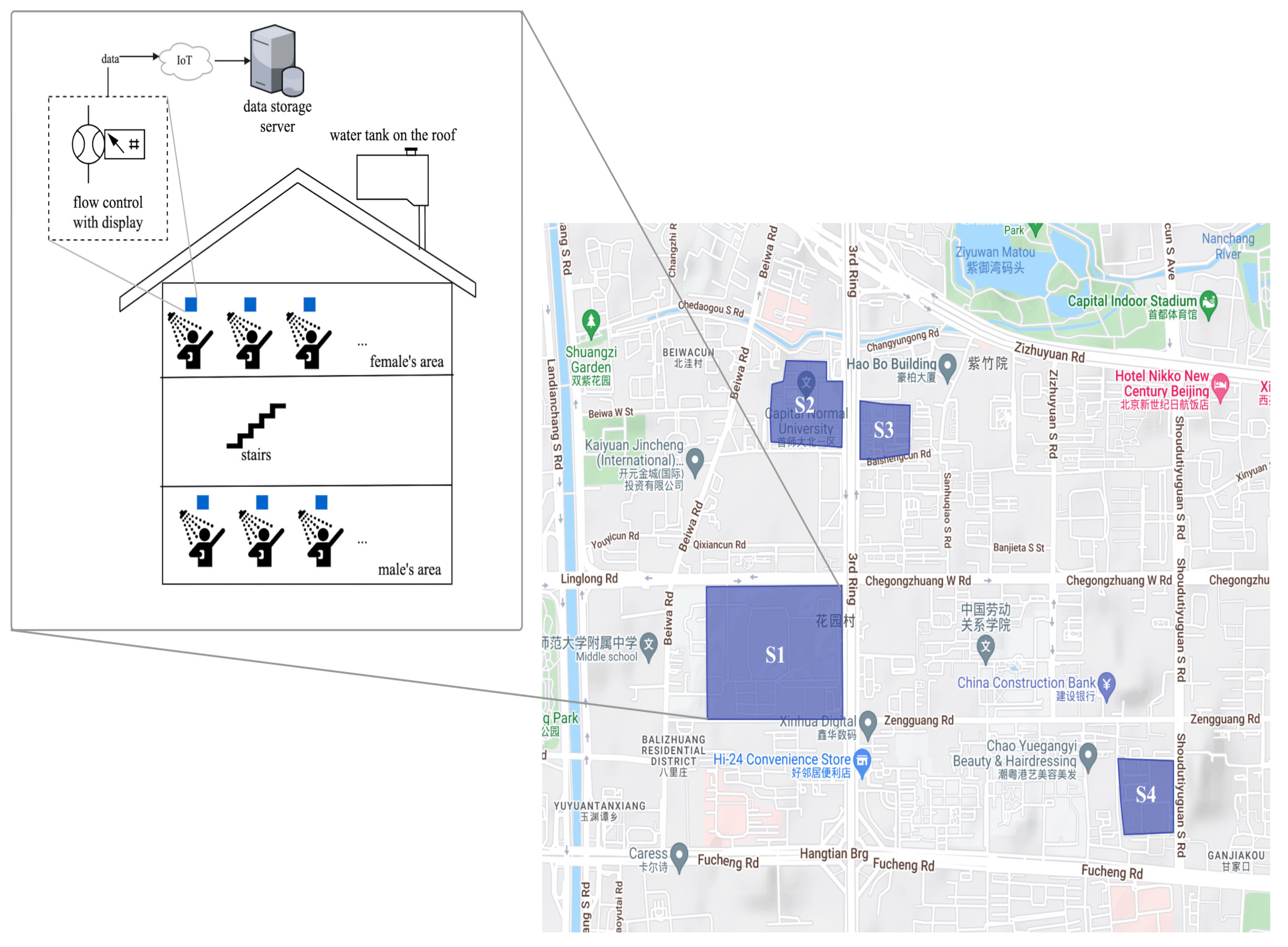
In this section, the available data are investigated to obtain a clear picture of the modeling task at hand. CNU is a comprehensive university in northern China administered by the Beijing Municipal Education Commission. Education, psychology, linguistics, and art are key fields of study at this university [56]. There are approximately 30,000 students divided into six campuses, each with a shower building near their dormitory. Almost all CNU students reside in school dormitories; therefore, BWD is a crucial component of the school’s water usage. As shown in Figure 2, every shower building includes separate areas for men and women. Since CNU’s male-to-female ratio is about 2:6, the female shower areas are busier and use more hot water than the male sections. Students swipe their campus ID cards prior to using the shower facility and water consumption is metered by a flow control device with an LED display next to the shower tap. At the time of study, the fee for water consumption was set at CNY 0.012/L. After being pumped and kept on top of the shower buildings, the bathwater is heated and then delivered. Shower rooms are open from 3:00 pm until 10:00 pm. Like most water demand time series data, bathwater consumption data are collected from the shower tap controller meter and the data are reported in real-time transaction-style to the bathwater management system through the IoT network for data storage and further analysis. For these reasons, short-term BWD forecasts are critical for the system’s efficient operation.

In this study, the bath water management system data for four shower buildings at CNU (Shower building ID: S1, S2, S3, S4) between 1 January 2017 and 31 December 2019 were obtained. A 10 min resample on the target scale was performed to pre-process the data for the analysis.

Table 1. Daily statistical information of the BWD data for shower areas.

# Shower	Area	Mean (L/Day)	Min (L/Day)	Max (L/Day)	Std. (L/Day)
S1	Female	162,191.30	59,559.98	267,326.00	35,371.21
	Male	58,067.52	83.60	85,420.80	11,269.02
S2	Female	103,048.70	20,454.41	189,537.10	35,092.80
	Male	24,412.12	4520.25	55,264.61	8456.39
S3	Female	74,287.67	139.70	144,388.90	21,161.10
	Male	29,347.84	46.25	51,045.32	8405.37
S4	Female	83,279.91	459.80	216,792.40	39,887.07
	Male	25,213.56	83.60	53,037.51	12,561.81

summarizes the daily statistical information for each shower area retrieved from the data server. Evidently, the part of the campus with shower building S1 had the highest bath water consumption.

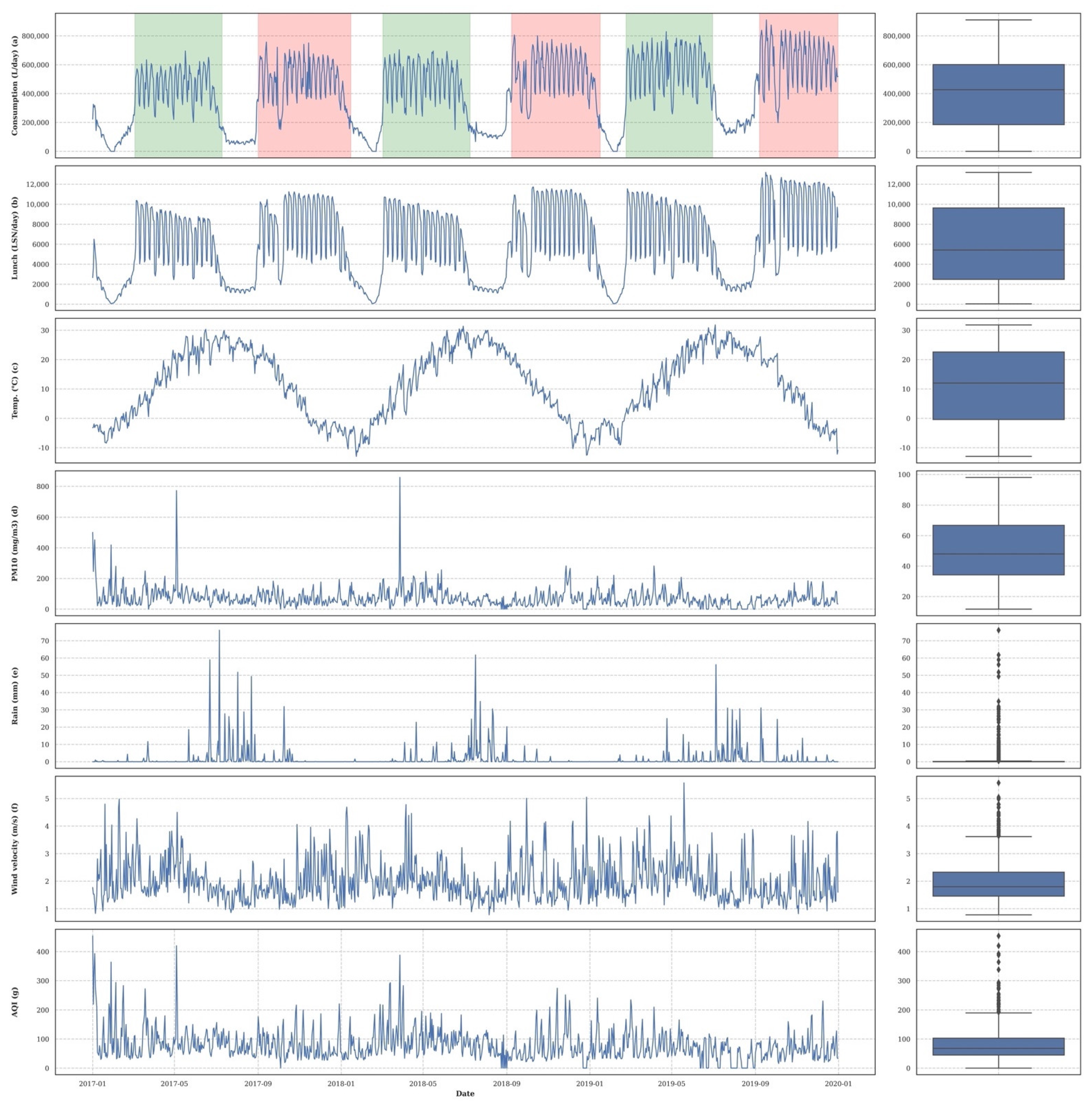
Early studies on urban water consumption have revealed that meteorological factors influence water demand [45,57]. Rathnayaka et al. [44] concluded that shower water use varies considerably between the seasons of summer and winter. Xenochristou et al. [57] showed that when weather factors are used as predictors during the summer months, the accuracy of water demand forecasting for homes with moderate occupancy and affluent occupants may be enhanced. In this study, to better forecast BWD, daily meteorological variables of Beijing, including daily average temperature (DAT), wind velocity (WV), precipitation (PCT), air quality index (AQI), and particulate matter 10 (PM10), were collected as covariates. Additionally, because shower rooms are accessible after lunch, we gathered the daily number of students (LSN) who have lunch at school in this study.

All these covariates are illustrated with the total BWD in Figure 3. In Figure 3a, the daily total BWD in spring terms (approximately from early March to late June) and autumn terms (approximately from early September to the next year’s mid-January) are highlighted with light green and light red backgrounds, respectively, while the unhighlighted portions indicate school vacations. During teaching days, BWD revealed a seasonal cycle of seven periods and a term cycle of around 18 weeks. Sharp increases and decreases in BWD are associated with the start and end of new terms, respectively. BWD showed higher stationarity during teaching days than during holidays (especially summer vacations and winter vacations). BWD also varied by day of the week, being lower on Fridays and higher on Sundays. To determine the significance of the covariates for the BWD, the Pearson correlation coefficient (PCC) [58] is examined. Results show that the PCC between the LSN and BWD was approximately 0.74 (Figure 3a,b), implying a strong correlation, while the PCCs between the BWD and DAT, WV, PCT, AQI, and PM10 are 0.09, −0.13, −0.23, −0.12 and −0.15, respectively, which means that the DAT has a positive relation with the BWD even though the relationship is weak; while the rest of the weather factors show a negative relationship with BWD, PCT shows a more negative relationship than the others (WV, AQI and PM10).

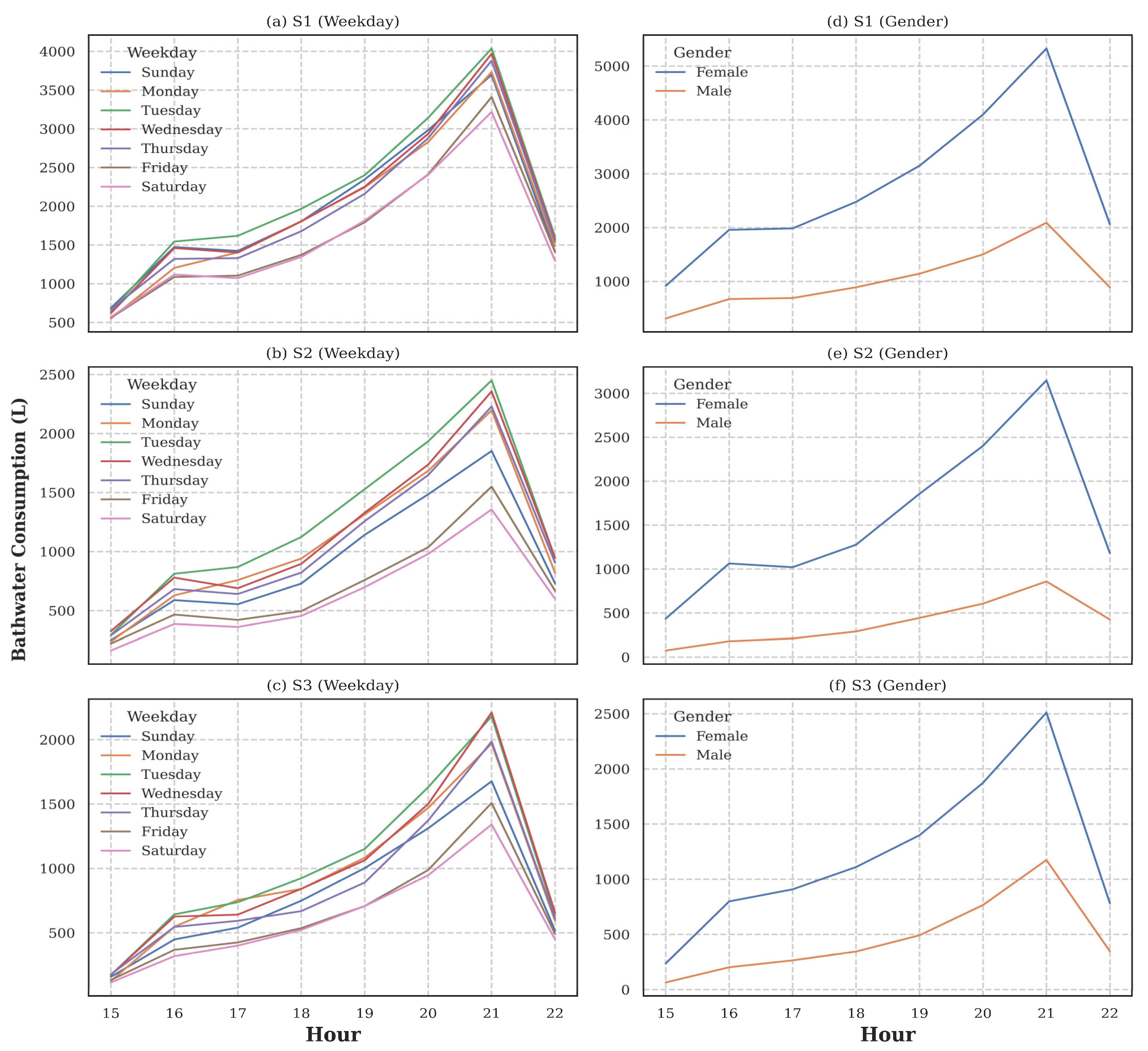
In addition, the hourly BWD of three shower buildings (S1, S2, and S3) was studied to obtain more information. As seen in Figure 4a–c, the average BWD on Tuesdays was higher than on other weekdays, while the lowest amount of bath water was consumed on Saturdays. This reveals that when all other factors are averaged, historical consumption and weekday appear to be one of the key driving elements, as discovered in [57]. Figure 4e,f show similar trends for all shower building areas. All subplots shown in Figure 4 imply that while some students take showers close to the opening time, many students take showers later in the evening.

3.4. Model Parameterizations

All modeling was performed in Python 3.8 using several Python packages. Pandas [59] (Version 1.4) was used to pre-process the raw data and Darts [60] (Version 0.16) was used to build the models for BWD forecasting. The inputs to the models were chosen based on the examination of the BWD data and covariates, as outlined in Section 3.3, and a grid search (GS) was conducted on all models to obtain the best performance. The selected inputs are described in

Table 2. Inputs of modes for daily and hourly time scale.

Models	Time Scale	Inputs and Outputs 1
ARIMA and ARMIAX	t = daily	$D_t=model\left(D_{t-1},D_{t-2},\dots ,D_{t-200}\right)$
	t = 1 h	$D_t=model\left(D_{t-1},D_{t-2},\dots ,D_{t-200},X_{t-1},X_{t-2},\dots ,X_{t-200}\right)$
RF	t = daily	$D_t=model\left(D_{t-1},D_{t-2},\dots ,D_{t-20},X_{t-1},X_{t-2},\dots ,X_{t-20}\right)$
	t = 1 h	$D_t=model\left(D_{t-1},D_{t-2},\dots ,D_{t-20},X_{t-1},X_{t-2},\dots ,X_{t-20}\right)$
LSTM	t = daily	$D_t=model\left(D_{t-1},D_{t-2},\dots ,D_{t-20},X_{t-1},X_{t-2},\dots ,X_{t-20}\right)$
	t = 1 h	$D_t=model\left(D_{t-1},D_{t-2},\dots ,D_{t-20},X_{t-1},X_{t-2},\dots ,X_{t-20}\right)$
N-BEATS	t = daily	$D_t=model\left(D_{t-1},D_{t-2},\dots ,D_{t-20},X_{t-1},X_{t-2},\dots ,X_{t-20}\right)$
	t = 1 h	$D_t=model\left(D_{t-1},D_{t-2},\dots ,D_{t-20},X_{t-1},X_{t-2},\dots ,X_{t-20}\right)$

¹$X$ contains all the selected covariates $\left\{LSN,DAT,PCT,PM10,WV,AQI,day of week,is\_holiday\right\}$.

. As shown in this table, to forecast the value of BWD at time $t$ ($D_t$), the inputs of the BWD of the previous $n$ consecutive ($D_{t-n}$) points were used. In particular, for the ARIMA and ARIMAX models, all previous points were used. Together with the BWD data, for the daily forecast purpose, the ARIMAX, RF, LSTM and N-BEATS models take the covariates (denoted with $X_{t-n}$ as inputs) aligned by time index to train the models, while for the hourly forecast purpose, the covariates were resampled to match the hourly dimension to train the models.

Originally, the GS is an exhaustive search across a chosen portion of the hyper parameter space [61]. The GS method evaluates all possible hyperparameter combinations and identifies the one that produces the greatest averaged validation score. It is simple and robust, as it considers all conceivable combinations. GS determined the best parameter set according to the mean absolute error. To calibrate the LSTM and N-BEATS models, a grid search was conducted to determine the hyperparameters, including the epoch, number of layers, learning rate, and batch size,

Table 3. Search range and optimized hyperparameters for the neural network models (LSTM, N-BEATS).

Model	Hyperparameters	Value Range	Best Hyperparameters
LSTM	Number of layers	{1, 2, 3, 4}	2
	dropout	{0, 0.2, 0.5}	0.2
	Learning rate	{0.001, 0.01, 0.1}	0.001
	Batch size	{32, 64, 96, 128}	32
	Number of iterations	{50, 100, 150, …, 500}	100
N-BEATS	Number of stacks	{1, 2, 3, 4}	2
	Number of blocks making up every stack	{2, 6, 10, 12}	10
	Number of layers	{1, 2, 3, 4}	2
	Learning rate	{0.001, 0.01, 0.1}	0.001
	Batch size	{32, 64, 96, 128}	32
	Number of iterations	{50, 100, 150, …, 500}	100

shows the parameter space and best parameter used in this study.

The method described by Tyralis et al. [62] was used to determine the maximum number of decision trees. The optimum hyperparameters for DL models were found using the grid search approach; a mini-batch size of 32; 0.001 (learning rate) and 100 (epochs) were found to be suitable, and MAE was utilized to measure loss during the model training. All candidate models were recalibrated for each shower room, since behavior varies among students in different campuses.

3.5. The Performance Evaluation Statistics

We chose four commonly used criteria to enable statistical analysis of model performance to estimate the forecast accuracy of our candidate models: MAPE, MAE, RMSE, and $R^2$. MAPE and root-mean-square error (RMSE) are two of the most often used statistics for measuring prediction error. Another kind of statistical indicator is the MAE statistic, which is used to measure the absolute error between observed and expected values. The coefficient R² indicates the degree to which predicted and actual data are linearly connected. Lower MAPE, MAE, and RMSE values indicate better model fits and larger $R^2$ values (from $-\infty$ to 1) represent better model performance. The MAPE is defined as in Equation (10):

$$\mathrm{MAPE}=\frac{1}{N}{\sum }_{𝑖=1}^N\left|\frac{Y_i-{\widehat{Y}}_i}{Y_i}\right|\times 100\%,$$

(10)

where N is the forecasted number of data points; $Y_i$ is the $i$th observed value; and ${\widehat{Y}}_i$ is the $i$th prediction value of the model. MAE is defined as:

$$\mathrm{MAE}=\frac{1}{N}{\sum }_{𝑖=1}^N\left|Y_i-{\widehat{Y}}_i\right|,$$

(11)

and $R^2$ is defined as:

$$R^2=\frac{{\left({\sum }_{𝑖=1}^N\left(Y_i-\tilde{Y}\right)\left(Y_i-\overline{Y}\right)\right)}^2}{{\sum }_{𝑖=1}^N{\left(Y_i-\tilde{Y}\right)}^2{\sum }_{𝑖=1}^N{\left(Y_i-\overline{Y}\right)}^2},$$

(12)

where $\overline{Y}$ is the mean of the observations and $\tilde{Y}$ is the mean of the prediction. The RMSE is defined as:

$$RMSE=\sqrt{\frac{{\sum }_{𝑖=1}^N\left(Y_i-{\widehat{Y}}_i\right)}{N}},$$

(13)

The target variable’s MAE and RMSE are stated in the same units.

4. Results and Discussion

Five models (ARIMA, ARIMAX, RF, LSTM, and N-BEATS) are compared based on four metrics: MAPE, RMSE, MAE, and R² in this section. For comparison, the results of daily and hourly BWD forecasts for each area are presented in Figure 5 and Figure 6 and

Table 4. MAPE-based performance evaluation of ARIMA, ARIMAX, LSTM, N-BEATS, and RF models (bold denotes correct findings for the corresponding shower room).

# Shower 1	MAPE (%)
	Area	ARIMA	ARIMAX	LSTM	N-BEATS	RF
S1	Female	8.29	8.37	5.79	8.23	7.43
	Male	7.67	7.52	7.45	8.99	6.44
S2	Female	21.94	13.97	10.16	13.01	9.34
	Male	12.31	12.16	27.6	14.65	18.05
S3	Female	13.22	11.96	7.42	8.34	10.38
	Male	11.82	10.87	9.36	8.63	10.52
S4	Female	34.19	22.27	7.14	9.90	7.63
	Male	19.64	12.73	18.30	7.99	8.79

¹ # Shower means the number of shower rooms.

,

Table 5. RMSE of models (bold indicates the best result for the corresponding shower room and gender).

# Shower	RMSE (L)
	Area	ARIMA	ARIMAX	LSTM	N-BEATS	RF
S1	Female	20,569.21	19,830.92	12,977.03	19,181.15	16,616.80
	Male	5608.95	6282.20	5793.31	6962.38	5199.88
S2	Female	29,163.63	17,157.82	14,632.48	18,039.73	13,717.48
	Male	2854.41	2577.66	5307.23	3387.84	3757.56
S3	Female	11,805.93	10,773.26	7163.36	8315.55	10,920.38
	Male	4148.97	3585.16	3232.50	3460.65	4048.87
S4	Female	28,951.02	18,730.00	6704.90	8543.52	9508.24
	Male	5990.95	4210.11	6310.59	3098.15	4088.29

,

Table 6. MAE of models (bold indicates the best result for corresponding shower room and gender).

# Shower	MAE (L)
	Area	ARIMA	ARIMAX	LSTM	N-BEATS	RF
S1	Female	15,032.80	15,729.62	10,875.18	14,646.27	13,663.45
	Male	4795.09	4605.77	4387.64	5391.32	3973.36
S2	Female	24,890.83	14,267.29	10,316.97	14,189.08	10,020.96
	Male	2320.85	2108.56	4826.66	2732.08	2805.59
S3	Female	10,090.04	8686.16	5557.70	6359.35	8409.56
	Male	2886.88	2843.58	2441.68	2441.96	2688.29
S4	Female	26,066.49	14,915.52	5500.95	7042.06	5598.26
	Male	4400.25	3525.62	5424.42	2317.34	2442.95

,

Table 7. R² of models (bold indicates the best result for the corresponding shower room and gender).

# Shower	R2
	Area	ARIMA	ARIMAX	LSTM	N-BEATS	RF
S1	Female	0.13	0.19	0.65	0.25	0.43
	Male	0.34	0.17	0.30	−0.02	0.43
S2	Female	−0.13	0.61	0.72	0.57	0.75
	Male	0.57	0.65	−0.49	0.39	0.25
S3	Female	0.36	0.47	0.77	0.68	0.46
	Male	0.56	0.67	0.73	0.70	0.58
S4	Female	−0.09	0.54	0.94	0.91	0.88
	Male	0.62	0.81	0.58	0.90	0.82

and

Table 8. Performance assessment with the models in terms of R² (bold indicates the best result for the corresponding shower room and gender).

# Shower	R2
	Area	ARIMA	ARIMAX	LSTM	N-BEATS	RF
S1	Female	0.52	0.88	0.75	0.73	0.88
	Male	0.20	0.78	0.79	0.70	0.62
S2	Female	−0.37	0.57	0.59	0.55	0.04
	Male	0.14	0.28	0.21	0.20	−0.59
S3	Female	−0.28	0.74	0.85	0.83	0.79
	Male	0.49	0.61	0.79	0.77	0.55
S4	Female	−0.25	0.68	0.85	0.82	0.21
	Male	−1.41	0.72	0.85	0.81	0.67

. Daily total BWD forecasts are also presented in terms of the stable supply of bath water in Figure 7 and

Table 9. Performance assessment for daily total BWD (bold indicates the best result for the corresponding shower room and gender).

Model	MAPE (%)	RMSE (L)	MAE (L)	R2
ARIMA	9.72	79,198.60	59,267.82	0.57
ARIMAX	10.99	88,816.73	69,310.27	0.45
LSTM	5.10	47,489.68	32,759.01	0.84
RF	6.27	60,036.64	38,912.98	0.75
N-BEATS	12.08	102,075.70	78,834.88	0.28

.

4.1. Daily BWD Forecasting

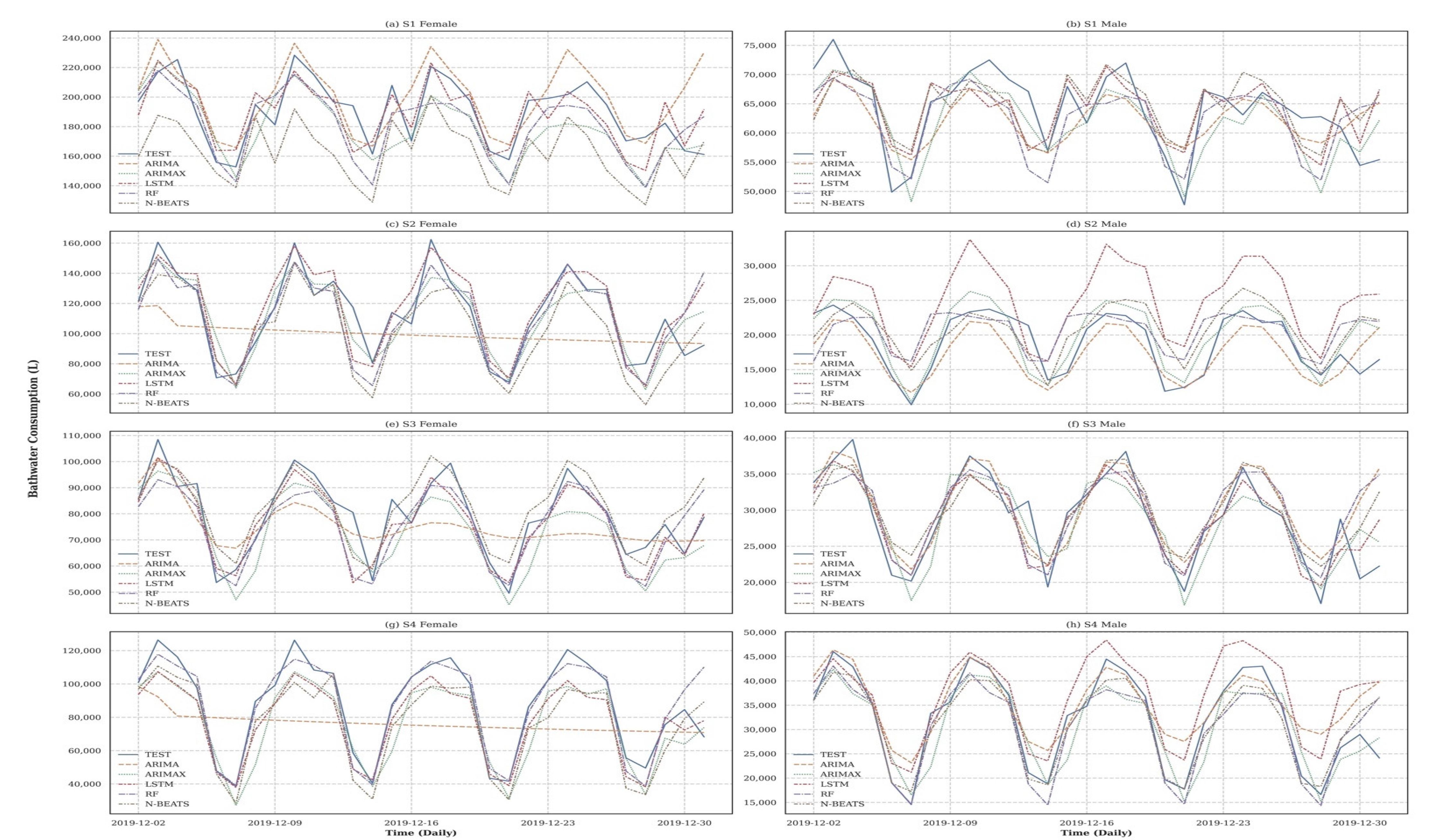
For four shower buildings (S1, S2, S3, S4), eight shower areas (female and male areas), and the actual and forecast results of daily ahead BWD using the ARIMA, ARIMAX, RF, LSTM, and N-BEATS models are illustrated in Figure 5a–h. BWD levels in different areas reflect different pattern characteristics. In terms of bath water consumption patterns, visual forecasting behavior differs between areas, even when the population, calendar, and climate factors are considered. The forecasted values were visually similar to the observed values (except for those with the ARIMA model). The ARIMA model achieved extremely poor forecast results as seen in Figure 5c,e,g, even with straight lines. Figure 5d shows that LSTM overestimated BWD. All subplots show that ARIMAX outperformed ARIMA for daily BWD forecast, which means that external factors affect BWD.

Table 4 summarizes the results of the daily BWD forecasting model. Evidently, the model with the best performance (MAPE = 5.79%) was LSTM, achieved for the S1 female area. The model performances of the female areas were better than those of the male areas, which means that the errors expressed as MAPE were smaller for shower rooms with higher water consumption. As Lin and Pai [63] proposed, the average MAPE values for industrial and commercial data may be interpreted as follows: 0% (very accurate forecasting), 10–20% (acceptable forecasting), 20–50% (decent forecasting), and >50% (inaccurate forecasting). The results showed that two ARIMA models, two ARIMAX models, five LSTM models, six N-BEATS models, and six RF models achieved highly accurate forecasting for all the shower room areas. The LSTM and N-BEATS models achieved the highest number of accurate forecasting results, whereas ARIMA and ARIMAX achieved only two accurate forecasts, both for shower room S1. The MAPE values imply that ML methods outperform statistical methods (particularly for larger datasets) and can be easily trained to fit more scenarios.

Table 5 and Table 6 summarize the RMSE and MAE results for the models. Lower RMSE and MAE values indicate that the modeled results were closer to the observed values. Table 4 showed the five models achieved highly accurate forecasts for shower room S1; however, when considering the RMSE and MAE indices, the LSTM model (RMSE = 12,977.03 L, MAE = 10,875.18 L) achieved the best results for female areas whereas the RF model (RMSE = 5199.88 L, MAE = 3973.36 L) achieved the best results for the male areas. For the male area of shower room S3, the N-BEATS model (MAPE = 8.63%) achieved better performance than the LSTM model (MAPE = 9.36%), as seen in Table 4. Comparing the RMSE and MAE in Table 5 and Table 6, the LSTM model (RMSE = 3232.50 L, MAE = 2441.68 L) achieved smaller deviation than the N-BEATS (RMSE = 3460.65 L, MAE = 2441.96 L) model.

R² values varied dramatically amongst shower rooms (Table 7). ARIMA obtained the lowest values (an average of 0.30 and even two negative values), indicating that BWD had a large number of random variables and so cannot be anticipated effectively for smaller regions.

Table 4 and Table 7 show that the LSTM (MAPE = 7.42%) and N-BEATS (MAPE = 8.34%) models of the female area with shower room S3 did not achieve highly accurate results, as opposed to the ARIMA, ARIMAX, and RF models (an MAPE > 10%). Evidently, results with high accuracy may be achieved by simply stacking the models with liner regression.

One of the study’s key findings is that machine learning technologies may significantly increase the management efficiency of CNU’s shared shower rooms. In a machine learning context, the no free lunch (NFL) theorem [64] implies that if a particular model is isolated for observation, it will definitely have less error addressing some issues and more error solving other issues; the results in this study also show that there is no single model that can be used for all sorts of shower rooms. As a result, it is critical to account for the computing resources, time, and knowledge necessary to find different ML-models to suit the BWD forecast for different shower areas.

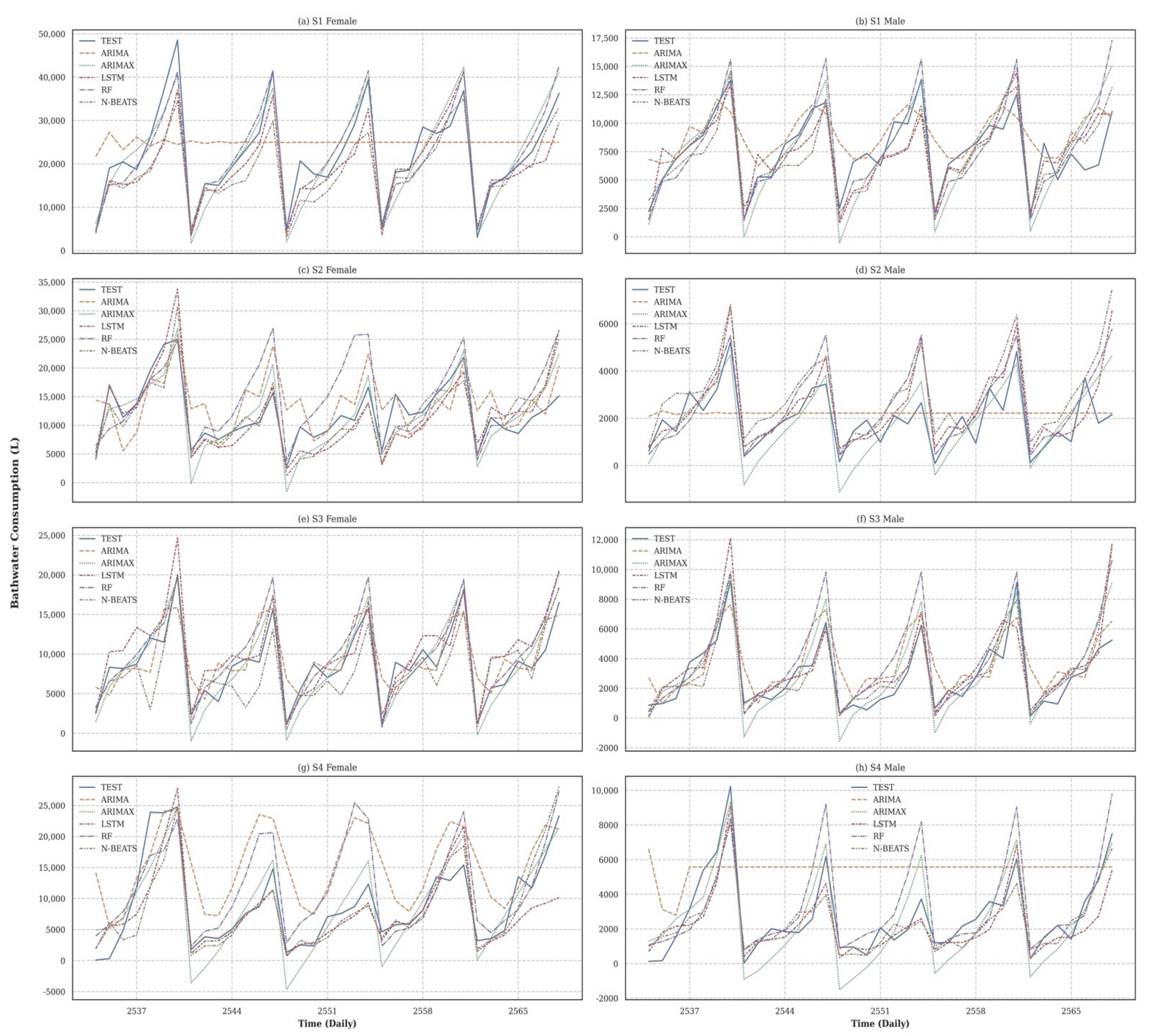
4.2. Hourly BWD Forecasting

The results of the hourly BWD forecasting for each area are illustrated in Figure 6 and Table 8 summarizes the R² metric.

Models based on DNN (LSTM and N-BEATS) forecasted the observed values better than statistical models (ARIMA and ARIMAX). The mean R² values in Table 8 indicate that the LSTM model (avg. R² = 0.71) achieved the best performance for hourly BWD forecasts. The ARIMA model achieved the worst performance (avg. R² < 0), which shows the weakness of statistical models for forecasting high-resolution time series forecast tasks by simply using historically observed BWD data; however, the ARIMAX model with covariates achieved a relatively high average R² value (avg. R² = 0.66).

4.3. Daily Total BWD Forecasting

The daily total BWD is important for bath water management. Figure 7 shows the forecast results for the five models. The forecast results were visually similar to the observed values for all models, which means that using total BWD may mitigate the impact of the varying BWD from different areas. Table 9 summarizes the metrics of daily total BWD, which shows that the LSTM model (MAPE = 5.10%, R² = 0.84) outperforms the other models, followed by RF (MAPE = 6.27%, R² = 0.75). The N-BEATS model (MAPE = 12.08%, R² = 0.28) achieved the worst performance. In addition, the ARIMA (MAPE = 9.72%, R² = 0.57) model achieved better results than those of the N-BEATS (MAPE = 12.08%, R² = 0.28) model, demonstrating that daily total BWD is more stationary for forecasting.

The choice of the model based on data availability and forecasting goals may significantly alter the results of the fine forecast (by area and hour). The models in this study were built using only 3 years of BWD data. Hence, our findings and results are ideal for situations with limited amounts of data; in contrasting situations, the models may leak some special events (e.g., rooms maintenance), rendering them incapable of accurate fine BWD forecasting. However, in terms of the high-accuracy (MAPE_LSTM = 5.10%) results summarized in Table 9, daily total BWD forecasting models can be employed to make bath water budget plans.

In summary, ML-based quantitative BWD forecast models with reasonable accuracy can be deployed instead of the managers’ empirical BWD estimate to improve bath water management efficiency; this would allow shower room managers to make better informed decisions about hot water heating and water pumping schedules, therefore saving energy. Bathwater heating and pumping can be planned in advance so that there is less water and energy wasted due to faulty empirical estimates.

Additionally, BWD trends may fluctuate over time, and student preferences may shift according to the seasons, course schedules or other reasons. Rather than deploying a model once, the models must be retrained if the data distributions differ considerably from those of the study’s initial training set.

5. Conclusions

This study explored the potential of the ARIMA, ARIMAX, RF, LSTM, and N-BEATS models for producing improved BWD forecasts in shared shower rooms for improving management efficiency, reducing energy and operating costs, and increasing student satisfaction. Calendar information, meteorological variables, and the number of students who took lunch were utilized as covariates to enhance the models’ accuracy. The following are the conclusions of BWD forecasting with machine learning models:

(1)

All models achieved good forecasting performance on daily total BWD in terms of accuracy. The management level of shared shower rooms is improved with accurate BWD forecasting results. Hence, the cost of heating and pumping bath water can be reduced. Furthermore, there is a large potential for energy savings as a consequence of accurate BWD forecasting in advance.

(2)

DNN models outperformed statistical models for daily and hourly BWD forecasting, whereas the LSTM models outperformed other models for high-resolution forecasting tasks.

(3)

In the event of a malfunction or sensor failure, missing data can be created using machine learning models with little resources and time utilizing historical data.

(4)

ML techniques can make campuses smarter, such as by forecasting canteen attendance and network flow consumption.

In summary, ML models can be applied to develop forecasting systems for smart campuses. In the future, we will work to fetch more external factors that affect BWD and obtain more BWD data to obtain improved forecasting performance.

References

- Rodriguez Rangel, H.; Puig, V.; Lopez Farias, R.; Flores, J.J. Short-Term Demand Forecast Using a Bank of Neural Network Models Trained Using Genetic Algorithms for the Optimal Management of Drinking Water Networks. J. Hydroinform. 2017, 19, 1–16. [Google Scholar] [CrossRef] [Green Version]
- Goh, P.S.; Ismail, A.F.; Ng, B.C.; Abdullah, M.S. Recent Progresses of Forward Osmosis Membranes Formulation and Design for Wastewater Treatment. Water 2019, 11, 2043. [Google Scholar] [CrossRef] [Green Version]
- Jagtap, S.; Skouteris, G.; Choudhari, V.; Rahimifard, S. Improving water efficiency in the beverage industry with the internet of things. In Implementing Data Analytics and Architectures for Next Generation Wireless Communications; IGI Global: Hershey, PA, USA, 2022; pp. 18–26. [Google Scholar]
- Eshoul, N.; Almutairi, A.; Lamidi, R.; Alhajeri, H.; Alenezi, A. Energetic, Exergetic, and Economic Analysis of MED-TVC Water Desalination Plant with and without Preheating. Water 2018, 10, 305. [Google Scholar] [CrossRef] [Green Version]
- Velarde, P.; Tian, X.; Sadowska, A.D.; Maestre, J.M. Scenario-Based Hierarchical and Distributed MPC for Water Resources Management with Dynamical Uncertainty. Water Resour. Manag. 2019, 33, 677–696. [Google Scholar] [CrossRef]
- Jagtap, S.; Skouteris, G.; Choudhari, V.; Rahimifard, S.; Duong, L.N.K. An Internet of Things Approach for Water Efficiency: A Case Study of the Beverage Factory. Sustainability 2021, 13, 3343. [Google Scholar] [CrossRef]
- Kim, D.; Kwon, D.; Park, L.; Kim, J.; Cho, S. Multiscale LSTM-Based Deep Learning for Very-Short-Term Photovoltaic Power Generation Forecasting in Smart City Energy Management. IEEE Syst. J. 2021, 15, 346–354. [Google Scholar] [CrossRef]
- Ruiz-Abellon, M.d.C.; Gabaldon, A.; Guillamon, A. Load Forecasting for a Campus University Using Ensemble Methods Based on Regression Trees. Energies 2018, 11, 2038. [Google Scholar] [CrossRef] [Green Version]
- Jung, S.-M.; Park, S.; Jung, S.-W.; Hwang, E. Monthly Electric Load Forecasting Using Transfer Learning for Smart Cities. Sustainability 2020, 12, 6364. [Google Scholar] [CrossRef]
- Yang, A.-M.; Li, S.-S.; Ren, C.-H.; Liu, H.-X.; Han, Y.; Liu, L. Situational Awareness System in the Smart Campus. IEEE Access 2018, 6, 63976–63986. [Google Scholar] [CrossRef]
- Wang, F.; Jia, Z. Constructing digital campus using campus smart card system. In Proceedings of the Instrumentation, Measurement, Circuits and Systems, Hangzhou, China, 16–18 April 2006; Zhang, T.B., Ed.; Springer: Berlin, Germany, 2012; Volume 127, pp. 19–26. [Google Scholar]
- Longo, E.; Sahin, F.A.; Redondi, A.E.C.; Bolzan, P.; Bianchini, M.; Maffei, S. A 5G-Enabled Smart Waste Management System for University Campus. Sensors 2021, 21, 8278. [Google Scholar] [CrossRef]
- Won, Y.-M.; Lee, J.-H.; Moon, H.-T.; Moon, Y.-I. Development and Application of an Urban Flood Forecasting and Warning Process to Reduce Urban Flood Damage: A Case Study of Dorim River Basin, Seoul. Water 2022, 14, 187. [Google Scholar] [CrossRef]
- Nunes Carvalho, T.M.; de Souza Filho, F.d.A.; Porto, V.C. Urban Water Demand Modeling Using Machine Learning Techniques: Case Study of Fortaleza, Brazil. J. Water Resour. Plan. Manage. ASCE 2021, 147, 05020026. [Google Scholar] [CrossRef]
- Mu, L.; Zheng, F.; Tao, R.; Zhang, Q.; Kapelan, Z. Hourly and Daily Urban Water Demand Predictions Using a Long Short-Term Memory Based Model. J. Water Resour. Plan. Manage. ASCE 2020, 146, 05020017. [Google Scholar] [CrossRef]
- Bakker, M.; van Duist, H.; van Schagen, K.; Vreeburg, J.; Rietveld, L. Improving the performance of water demand forecasting models by using weather input. In Proceedings of the 12th International Conference on Computing and Control for the Water Industry, Ccwi2013, Perugia, Italy, 2–4 September 2013; Brunone, B., Giustolisi, O., Ferrante, M., Laucelli, D., Meniconi, S., Berardi, L., Campisano, A., Eds.; Elsevier Science BV: Amsterdam, The Netherlands, 2014; Volume 70, pp. 93–102. [Google Scholar]
- Chaiyasen, B.; Makpiboon, C.; Pornprommin, A.; Lipiwattanakarn, S. Temporal Scale Impacts of Weather Variables on Urban Water Demand. Suranaree J. Sci. Technol. 2021, 28, 71–77. [Google Scholar]
- Makpiboon, C.; Pornprommin, A.; Lipiwattanakarn, S. Impacts of Weather Variables on Urban Water Demand at Multiple Temporal Scales. Int. J. GEOMATE 2020, 18, 71–77. [Google Scholar] [CrossRef]
- Protopapas, A.L.; Katchamart, S.; Platonova, A. Weather Effects on Daily Water Use in New York City. J. Hydrol. Eng. 2000, 5, 332–338. [Google Scholar] [CrossRef]
- Koo, K.-M.; Han, K.-H.; Jun, K.-S.; Lee, G.; Kim, J.-S.; Yum, K.-T. Performance Assessment for Short-Term Water Demand Forecasting Models on Distinctive Water Uses in Korea. Sustainability 2021, 13, 6056. [Google Scholar] [CrossRef]
- Xenochristou, M.; Hutton, C.; Hofman, J.; Kapelan, Z. Short-Term Forecasting of Household Water Demand in the UK Using an Interpretable Machine Learning Approach. J. Water Resour. Plan. Manage. ASCE 2021, 147, 04021004. [Google Scholar] [CrossRef]
- Oreshkin, B.N.; Dudek, G.; Pelka, P.; Turkina, E. N-BEATS Neural Network for Mid-Term Electricity Load Forecasting. Appl. Energy 2021, 293, 116918. [Google Scholar] [CrossRef]
- Mo, R.; Xu, B.; Zhong, P.; Zhu, F.; Huang, X.; Liu, W.; Xu, S.; Wang, G.; Zhang, J. Dynamic Long-Term Streamflow Probabilistic Forecasting Model for a Multisite System Considering Real-Time Forecast Updating through Spatio-Temporal Dependent Error Correction. J. Hydrol. 2021, 601, 126666. [Google Scholar] [CrossRef]
- Chen, H.; Xu, Y.-P.; Teegavarapu, R.S.; Guo, Y.; Xie, J. Assessing Different Roles of Baseflow and Surface Runoff for Long-Term Streamflow Forecasting in Southeastern China. Hydrol. Sci. J. 2021, 66, 2312–2329. [Google Scholar] [CrossRef]
- Kuehnert, C.; Gonuguntla, N.M.; Krieg, H.; Nowak, D.; Thomas, J.A. Application of LSTM Networks for Water Demand Prediction in Optimal Pump Control. Water 2021, 13, 644. [Google Scholar] [CrossRef]
- Bai, Y.; Wang, P.; Li, C.; Xie, J.; Wang, Y. Dynamic Forecast of Daily Urban Water Consumption Using a Variable-Structure Support Vector Regression Model. J. Water Resour. Plan. Manage. ASCE 2015, 141, 04014058. [Google Scholar] [CrossRef]
- Almanei, M.; Oleghe, O.; Jagtap, S.; Salonitis, K. Machine Learning Algorithms Comparison for Manufacturing Applications; IOS Press: Amsterdam, The Netherlands, 2021. [Google Scholar]
- Do, N.C.; Simpson, A.R.; Deuerlein, J.W.; Piller, O. Particle Filter-Based Model for Online Estimation of Demand Multipliers in Water Distribution Systems under Uncertainty. J. Water Resour. Plan. Manage. ASCE 2017, 143, 04017065. [Google Scholar] [CrossRef] [Green Version]
- Kofinas, D.; Mellios, N.; Papageorgiou, E.; Laspidou, C. Urban water demand forecasting for the island of Skiathos. In Proceedings of the 16th Water Distribution System Analysis Conference (wdsa2014): Urban Water Hydroinformatics and Strategic Planning, Bari, Italy, 14–17 July 2014; Giustolisi, O., Brunone, B., Laucelli, D., Berardi, L., Campisano, A., Eds.; Elsevier Science BV: Amsterdam, The Netherlands, 2014; Volume 89, pp. 1023–1030. [Google Scholar]
- Wong, J.S.; Zhang, Q.; Chen, Y.D. Statistical Modeling of Daily Urban Water Consumption in Hong Kong: Trend, Changing Patterns, and Forecast. Water Resour. Res. 2010, 46, W03506. [Google Scholar] [CrossRef]
- Hutton, C.J.; Kapelan, Z. A Probabilistic Methodology for Quantifying, Diagnosing and Reducing Model Structural and Predictive Errors in Short Term Water Demand Forecasting. Environ. Modell. Softw. 2015, 66, 87–97. [Google Scholar] [CrossRef]
- Quevedo, J.; Saludes, J.; Puig, V.; Blanch, J. Short-term demand forecasting for real-time operational control of the Barcelona water transport network. In Proceedings of the 2014 22nd Mediterranean Conference on Control and Automation (med), Palermo, Italy, 31 May–2 June 2014; IEEE: New York, NY, USA, 2014; pp. 990–995. [Google Scholar]
- Huntra, P.; Keener, T.C. Evaluating the Impact of Meteorological Factors on Water Demand in the Las Vegas Valley Using Time-Series Analysis: 1990–2014. ISPRS Int. Geo Inf. 2017, 6, 249. [Google Scholar] [CrossRef] [Green Version]
- Candelieri, A.; Giordani, I.; Archetti, F.; Barkalov, K.; Meyerov, I.; Polovinkin, A.; Sysoyev, A.; Zolotykh, N. Tuning Hyperparameters of a SVM-Based Water Demand Forecasting System through Parallel Global Optimization. Comput. Oper. Res. 2019, 106, 202–209. [Google Scholar] [CrossRef]
- Brentan, B.M.; Luvizotto, E.; Herrera, M.; Izquierdo, J.; Perez-Garcia, R. Hybrid Regression Model for near Real-Time Urban Water Demand Forecasting. J. Comput. Appl. Math. 2017, 309, 532–541. [Google Scholar] [CrossRef]
- Herrera, M.; Torgo, L.; Izquierdo, J.; Perez-Garcia, R. Predictive Models for Forecasting Hourly Urban Water Demand. J. Hydrol. 2010, 387, 141–150. [Google Scholar] [CrossRef]
- Mouatadid, S.; Adamowski, J. Using Extreme Learning Machines for Short-Term Urban Water Demand Forecasting. Urban Water J. 2017, 14, 630–638. [Google Scholar] [CrossRef]
- Braun, M.; Bernard, T.; Piller, O.; Sedehizade, F. 24-hours demand forecasting based on SARIMA and support vector machines. In Proceedings of the 16th Water Distribution System Analysis Conference (wdsa2014): Urban Water Hydroinformatics and Strategic Planning, Bari, Italy, 14–17 July 2014; Giustolisi, O., Brunone, B., Laucelli, D., Berardi, L., Campisano, A., Eds.; Elsevier Science BV: Amsterdam, The Netherlands, 2014; Volume 89, pp. 926–933. [Google Scholar]
- Kiranyaz, S.; Ince, T.; Iosifidis, A.; Gabbouj, M. Operational Neural Networks. Neural Comput. Appl. 2020, 32, 6645–6668. [Google Scholar] [CrossRef] [Green Version]
- Lockner, Y.; Hopmann, C. Induced Network-Based Transfer Learning in Injection Molding for Process Modelling and Optimization with Artificial Neural Networks. Int. J. Adv. Manuf. Technol. 2021, 112, 3501–3513. [Google Scholar] [CrossRef]
- Vijai, P.; Sivakumar, B.P. Performance comparison of techniques for water demand forecasting. In Proceedings of the 8th International Conference on Advances in Computing & Communications (icacc-2018), Kochi, India, 13–15 September 2018; Buyya, R., Sherly, K.K., Eds.; Elsevier Science BV: Amsterdam, The Netherlands, 2018; Volume 143, pp. 258–266. [Google Scholar]
- Xenochristou, M.; Kapelan, Z. An Ensemble Stacked Model with Bias Correction for Improved Water Demand Forecasting. Urban Water J. 2020, 17, 212–223. [Google Scholar] [CrossRef]
- Yanhui, D.; Weibo, Z. Urban residential water demand forecasting in Xi’an based on RBF model. In Proceedings of the Iceet: 2009 International Conference on Energy and Environment Technology—Volume 2, Proceedings, Guilin, China, 16–18 October 2009; IEEE Computer Soc.: Los Alamitos, CA, USA, 2009; pp. 901–904. [Google Scholar]
- Rathnayaka, K.; Malano, H.; Maheepala, S.; George, B.; Nawarathna, B.; Arora, M.; Roberts, P. Seasonal Demand Dynamics of Residential Water End-Uses. Water 2015, 7, 202–216. [Google Scholar] [CrossRef] [Green Version]
- Banjac, G.; Vasak, M.; Baotic, M. Adaptable Urban Water Demand Prediction System. Water Sci. Technol. Water Supply 2015, 15, 958–964. [Google Scholar] [CrossRef]
- Cutore, P.; Campisano, A.; Kapelan, Z.; Modica, C.; Savic, D. Probabilistic Prediction of Urban Water Consumption Using the SCEM-UA Algorithm. Urban Water J. 2008, 5, 125–132. [Google Scholar] [CrossRef]
- House-Peters, L.A.; Chang, H. Urban Water Demand Modeling: Review of Concepts, Methods, and Organizing Principles. Water Resour. Res. 2011, 47. [Google Scholar] [CrossRef] [Green Version]
- Rahim, M.S.; Nguyen, K.A.; Stewart, R.A.; Ahmed, T.; Giurco, D.; Blumenstein, M. A Clustering Solution for Analyzing Residential Water Consumption Patterns. Knowledge Based Syst. 2021, 233, 107522. [Google Scholar] [CrossRef]
- Makki, A.A.; Stewart, R.A.; Panuwatwanich, K.; Beal, C. Revealing the Determinants of Shower Water End Use Consumption: Enabling Better Targeted Urban Water Conservation Strategies. J. Clean Prod. 2013, 60, 129–146. [Google Scholar] [CrossRef] [Green Version]
- Viccione, G.; Guarnaccia, C.; Mancini, S.; Quartieri, J. On the Use of ARIMA Models for Short-Term Water Tank Levels Forecasting. Water Supply 2020, 20, 787–799. [Google Scholar] [CrossRef] [Green Version]
- Islam, F.; Imteaz, M.A. Use of Teleconnections to Predict Western Australian Seasonal Rainfall Using ARIMAX Model. Hydrology 2020, 7, 52. [Google Scholar] [CrossRef]
- Hochreiter, S.; Schmidhuber, J. Long Short-Term Memory. Neural Comput. 1997, 9, 1735–1780. [Google Scholar] [CrossRef] [PubMed]
- Breiman, L. Random Forests. Mach. Learn. 2001, 45, 5–32. [Google Scholar] [CrossRef] [Green Version]
- Dudek, G. Short-term load forecasting using random forests. In Proceedings of the Intelligent Systems’2014, Volume 2: Tools, Architectures, Systems, Applications, Warsaw, Poland, 24–26 September 2014; Filev, D., Jablkowski, J., Kacprzyk, J., Krawczak, M., Popchev, I., Rutkowski, L., Sgurev, V., Sotirova, E., Szynkarczyk, P., Zadrozny, S., Eds.; Springer: Berlin, Germany, 2015; Volume 323, pp. 821–828. [Google Scholar]
- Putz, D.; Gumhalter, M.; Auer, H. A Novel Approach to Multi-Horizon Wind Power Forecasting Based on Deep Neural Architecture. Renew. Energy 2021, 178, 494–505. [Google Scholar] [CrossRef]
- Basic Info—Capital Normal University. Available online: https://www.cnu.edu.cn/xxgk/sjsd/jbqk/index.htm (accessed on 26 January 2022).
- Xenochristou, M.; Kapelan, Z.; Hutton, C.; Hofman, J. Smart Water Demand Forecasting: Learning from the Data. EPiC Ser. Eng. 2018, 3, 2351–2358. [Google Scholar]
- Feng, W.; Zhu, Q.; Zhuang, J.; Yu, S. An Expert Recommendation Algorithm Based on Pearson Correlation Coefficient and FP-Growth. Cluster Comput. 2019, 22, S7401–S7412. [Google Scholar] [CrossRef]
- Pandas—Python Data Analysis Library. Available online: https://pandas.pydata.org/ (accessed on 16 February 2022).
- Herzen, J.; Lässig, F.; Piazzetta, S.G.; Neuer, T.; Tafti, L.; Raille, G.; van Pottelbergh, T.; Pasieka, M.; Skrodzki, A.; Huguenin, N.; et al. Darts: User-Friendly Modern Machine Learning for Time Series. arXiv 2021, arXiv:2110.03224. [Google Scholar]
- Bzdok, D.; Altman, N.; Krzywinski, M. Points of Significance Statistics versus Machine Learning. Nat. Methods 2018, 15, 232–233. [Google Scholar] [CrossRef]
- Tyralis, H.; Papacharalampous, G. Variable Selection in Time Series Forecasting Using Random Forests. Algorithms 2017, 10, 114. [Google Scholar] [CrossRef] [Green Version]
- Lin, K.-P.; Pai, P.-F. Solar Power Output Forecasting Using Evolutionary Seasonal Decomposition Least-Square Support Vector Regression. J. Clean. Prod. 2016, 134, 456–462. [Google Scholar] [CrossRef]
- Gómez, D.; Rojas, A. An Empirical Overview of the No Free Lunch Theorem and Its Effect on Real-World Machine Learning Classification. Neural Comput. 2016, 28, 216–228. [Google Scholar] [CrossRef] [PubMed] [Green Version]
Figure 1.
Diagram illustration of BWD forecasting and performance assessment.
Figure 2.
Distribution and architecture of shower buildings: S1 serves the largest area while S3 serves the smallest area in the campus.
Figure 3.
Relationship between BWD and covariates: (a) bath water consumption, (b) number of students who take lunch, (c) average temperature, (d) PM10, (e) rain, (f) wind velocity, and (g) air quality index (AQI).
Figure 4.
Hourly bath water demand (BWD) by (a–c) weekday and (d–f) gender.
Figure 5.
Comparison of observed and forecasted daily BWD of each shower room with ARIMA, ARIMAX, LSTM, RF, and N-BEATS models, (a,c,e,g) for female rooms, (b,d,f,h) for male rooms.
Figure 6.
Illustration of the observed and forecasted values for hourly BWD of each shower room using ARIMA, ARIMAX, LSTM, RF, and N-BEATS models, (a,c,e,g) for female areas, (b,d,f,h) for male areas.
Figure 7.
Daily total BWD forecast results using ARIMA, ARIMAX, LSTM, RF, and N-BEATS models.