
Ecosystem Service Assessment of Soil and Water Conservation Based on Scenario Analysis in a Hilly Red-Soil Catchment of Southern China


1
Institute of Intelligent Media Technology, Communication University of Zhejiang, Hangzhou 310018, China
2
Key Laboratory of Water Cycle and Related Land Surface Processes, Institute of Geographic Sciences and Natural Resources Research, Chinese Academy of Sciences, Beijing 100101, China
3
College of Media Engineering, Communication University of Zhejiang, Hangzhou 310018, China
*
Author to whom correspondence should be addressed.
Water 2022, 14(8), 1284; https://doi.org/10.3390/w14081284
Submission received: 27 February 2022
/
Revised: 12 April 2022
/
Accepted: 13 April 2022
/
Published: 15 April 2022
(This article belongs to the Special Issue Effect of Soil Erosion on the Water Environment)
Abstract
:Soil and water conservation (SWC) practices on agricultural watersheds have been the most effective practices for preventing soil erosion for several decades. The ecosystem services (ES) protected or enhanced by SWC practices include the comprehensive effects of protecting and conserving water sources, protecting and improving soil, carbon fixation, increasing agricultural production, and so on. Due to the lack of ES evaluation indicators and unified calculation methods in line with regional characteristics, this study proposes a framework of scenario analysis by using ES mapping, ES scoring, and economic analysis technology for ES and economic-benefit trade-offs under different scenarios. The study area was the Xiaoyang catchment located in Ningdu County, Jiangxi Province, which is a typically hilly red-soil region of southern China. From the results of scenario analysis, an obvious phenomenon is that some SWC practices can affect the value of some ES indicators, while some have no clear trend. By computing the ES scores for the four scenarios, the ranking was S3 (balanced), S1 (conservation), S2 (economic), and S0 (baseline). S3 ranks second in net income (with CNY 4.73 million), preceded only by S2 (CNY 6.36 million). Based on the above rankings, S3 is the relatively optimal scenario in this study. The contributions of this study are the method innovation with the localization or customized selection of ES indicators, and scenario analysis with ES scores and economic-benefit trade-offs in different scenarios.
1. Introduction
The distribution area of red soil in hilly areas of southern China is large. Due to the limited cultivated land resources and the huge demand of local people for living resources, the conflict between humans and land is more prominent in these areas [1,2,3]. As a result, soil erosion has been serious in the hilly red-soil region of southern China over the past several decades. Serious soil erosion also deteriorates rural environments and hinders the implementation of policies aimed at to achieving common prosperity. What is the impact of soil erosion on the environment and economy? It is hard to answer this clearly. Soil and water conservation (SWC) or agricultural best management practices (BMP) can alleviate soil erosion and bring benefits to both humans and the environment [4]. Ecosystem services (ES), the benefits that humans obtain from nature, are of great importance for human well-being, and can ideally be measured by ES assessments [5]. Agricultural conservation practices change soil properties and processes and affect the underlying biodiversity. These changes can, in turn, affect the delivery of ecosystem services [6]. Therefore, scenario analysis technology can help analyze changes in soil properties and biodiversity caused by agricultural conservation practices as viewed from the perspective of ES.
Ecosystem services (ES) are functions provided by the environment that benefit humans; they can be classified as provisioning, regulating, supporting, or cultural services [7]. The provision of food is a primary function and key ecosystem service of agriculture. However, in many cases, people are not aware of the benefits of ES in both environmental and economic contexts. Thus, to better recognize the multiple benefits, several studies have conducted economic and ecological assessments of ES [8,9,10,11]. An important research direction in this field is the monetization of ES and the quantification of environmental benefits. There are three methods for the monetization of ES. One is the revealed-preference approach, such as travel cost, market methods, hedonic methods, and production approaches. The second is the stated-preference approach, such as contingent valuation and conjoint analysis. The last one is a cost-based approach, including replacement and avoidance cost. The individual index-based methods and group-based methods are the methods of non-monetizing valuation or assessment. Spatially explicit functional modeling is a more and more popular method for the environmental quantification of ES. Modeling at a scale appropriate for land management, for instance, farm scales, provides important information about farmer choice and decision making. There are several models and frameworks that can be aggregated and scaled up to cover whole landscapes and regions, as well as on national and global levels. However, no one model or framework will work for all purposes [12].
Land-use change leads to land-cover change, which has important impacts on hydrological processes and water ecology [11,13,14]; thus, many studies focus on the change in ES value caused by land-use change [15,16,17,18,19]. Soil and water conservation (SWC) practices can reduce soil erosion and water runoff, thus conserving soil, and those practices include buffer strip, conservation tillage (reduced tillage or no-till), permanent organic soil cover by retaining crop residues, crop rotations, cover crops, and other structural practices [20]. Like the land-use change, the change of ES is most likely to be affected by SWC practices. Some practices can decrease ES delivery (tradeoffs); others can enhance or maintain ES (synergies) [6]. It is important to understand the relationship between SWC and ES, which is increasingly recognized by scientists and policymakers [21,22]. Therefore, it is necessary to map ecosystem services on these conservation practices [23]. However, this is not a small challenge due to the complexity of ES trade-offs as well as spatial and temporal variation in different conservation contexts. There are few studies presented in this field.
Scenario analysis is currently one of the most common methods used in ES trade-off and synergy studies [24,25,26,27]. By setting up alternative land use or climate change scenarios and calculating the changes in and interactions among ES, this method can provide a trade-off of various situations for policymaking [28]. There are some studies on ecosystem service assessment of soil and water conservation using the scenario analysis method [29,30,31,32]. However, there are still some limitations on previous studies. First, the indicators of ES evaluated by the existing model are limited, and it is difficult to calculate those important local ecological service indicators. Second, for the multi-dimensional results reflected by multiple indicators of ES, due to the interaction and mutual restraint between indicators [33], it is difficult to clarify the causal relationship or process of them, but only the correlation. Another challenge is that all too often, the data that are utilized to parameterize ES models represents these processes coarsely, and consequently, the ES services, may be poorly represented [34]. As a result, without validation efforts, it may be difficult for others to accept the simplifying assumptions, thereby failing to meet the needs of scientific decision making [25]. Fourth, due to the difference in regional environment, climatic conditions, and human activities, these general methods still need to be verified, and they need to be constantly revised to adapt to different regions. For example, tillage practices are primarily applied on large-scale, mechanized farms in America, and require large applications of herbicides to control weeds, while in hilly red-soil areas in the south of China, these practices are applied mainly on small-scale, non-mechanized agricultural fields. Decision makers and scientists need to know the specific places where ES trade-offs and synergies occur. However, few studies have improved and applied the general method locally.
Thirty years ago, the policy of SWC changed from production and economy to ecosystem benefits in hilly red-soil regions of southern China. The characteristics of hilly red-soil regions are: (1) high erodibility due to the climatic and environmental conditions, such as extreme rainfall events, geology, topography, vegetation, physical and chemical soil properties, etc.; (2) closely related to local fragile ecology and low economic development; and (3) the regional particularity of soil and water conservation targets, which should not only prevent soil erosion but also take into account ecological protection and economic development. In order to narrow the knowledge gap between ecosystem benefits and conservation decision making, this paper selects the small catchment in Jiangxi Province as the study area, and fully considers the characteristics of hilly red-soil regions of southern China.
Specifically, the main tasks of this paper were to: (1) define a framework of scenario analysis process for ES assessment for the hilly red-soil region of southern China; (2) design scenarios of soil and water conservation unique to the study area; (3) evaluate changes in the local typical ecosystem services in each scenario, such as runoff regulation, soil conservation, and fruit and fishery production; (4) determine the optimal scenario based on ecosystem services and economic-benefit trade-offs in different scenarios.
2. Methods
2.1. Study Area and Data Sources
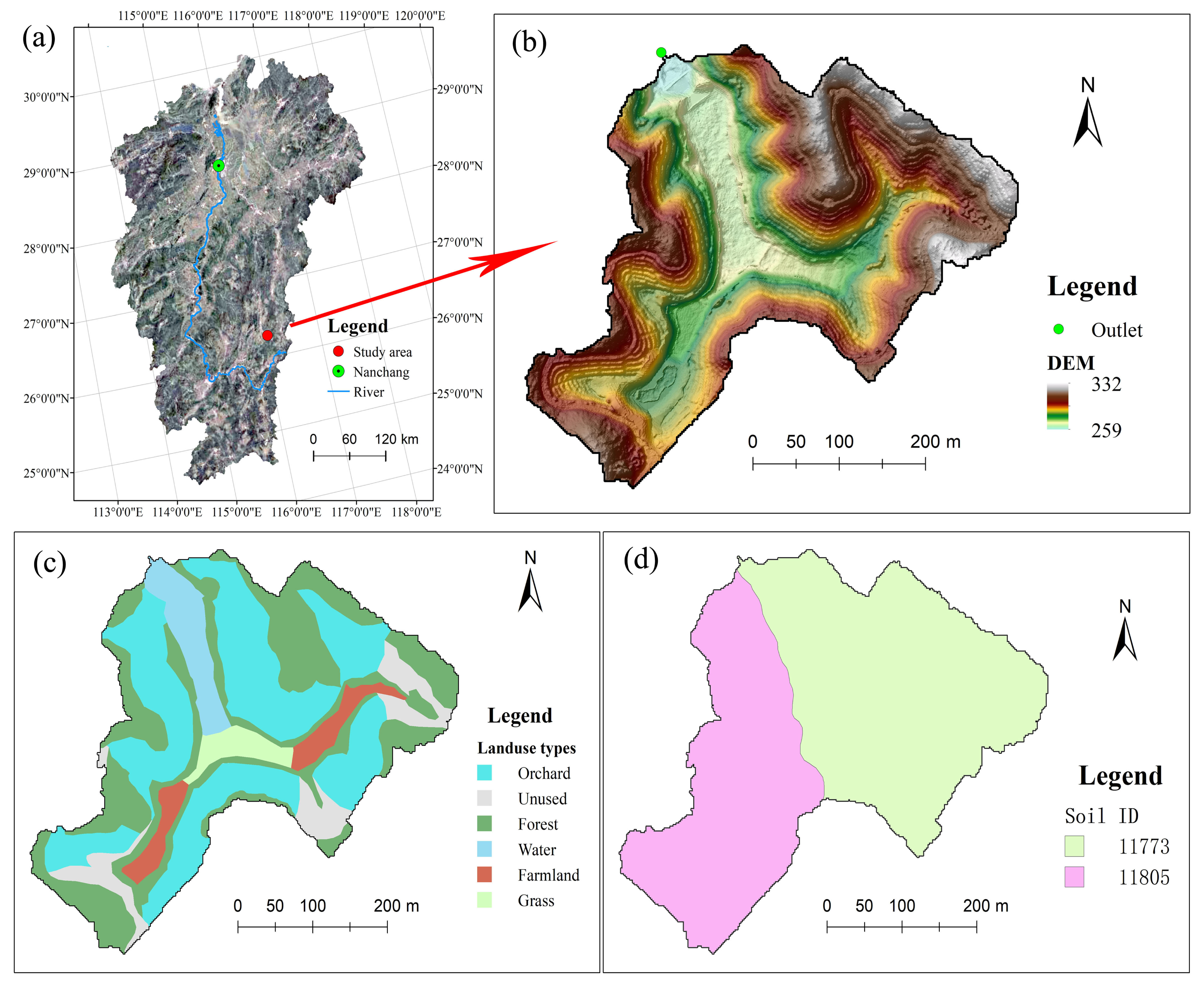
In this study, a small catchment was selected in the Xiaoyang watershed of Ningdu County, Jiangxi Province, China. The Xiaoyang watershed is downstream of the first tributary of Meijiang River, which is one of the five major rivers in the water system of Poyang Lake. The small catchment, with an area of 0.145 km2, as shown in Figure 1a, is the core demonstration area of Xiaoyang watershed for the soil and water conservation project of efficient development management. The watershed can be divided into several geomorphic categories, including hills, valley plains, and rivers. The terrain fluctuates greatly with an elevation between 259 and 332 m, as shown in Figure 1b. Approximately 50% of land use is forest land, 9.5% is comprised of water bodies, and 21% is farmland and grass (Figure 1c). There are two soil types in the study area, with the soil IDs linked to the Harmonized World Soil Database for soil physico-chemical properties, such as texture, bulk density, organic carbon, and so on (Figure 1d). The annual average temperature is 18.9 °C, with an extreme maximum temperature of 38.6 °C and extreme minimum temperature of –6.3 °C. The annual average precipitation is 1550.6 mm. The annual average evaporation is 1557.8 mm, and the annual average runoff depth is 1032 mm. Precipitation is concentrated from April to August (see Figure 2), and often in the form of storms. For example, the precipitation was 187.4 mm on 18 May 2015. Water erosion is the main type of soil erosion, and the annual soil erosion modulus is 2796 t/km2·a. As the study area is relatively small, it is easier to design spatially fine scenarios using expert knowledge, and it is convenient to map and calculate ES more clearly and locally.
The data used in this study were from official websites and field investigations. The data mainly included: a digital elevation model (DEM), land-use classifications, and precipitation data, obtained from the Resource and Environment Data Cloud Platform (REDCP, http://www.resdc.cn (accessed on 26 February 2022)); soil data were from the Harmonized World Soil Database (http://webarchive.iiasa.ac.at/Research/LUC/External-World-soil-database (accessed on 26 February 2022)) and economic data of soil and water conservation were collected by field investigations in 2019 and obtained from the local statistical yearbook of 2017. Land use data for scenario design were derived from the digital map of land use in 2015 and aerial image data from UAV (unmanned aerial vehicle) imaging in 2018 and 2019. Soil property data were obtained from laboratory measurements. Local species were obtained from field investigations. Detailed descriptions of the data are shown in Table 1. The DEM and land use map with a grid size of 2 m derived from UAV data were verified by the DEM and land use map with a grid size of 30 m from REDCP to ensure the accuracy of the data. At the same time, the field investigation could also play a role in this regard.
2.2. Soil and Water Conservation Practices
Over the past 30 years, with the great attention paid to soil and water conservation, farmers and technicians have made unremitting efforts to carry out improved management practices locally and have successfully found a way to prevent and control soil erosion under regional characteristics. Abundant experience was accumulated, and several conservation management practices were refined for the study area. These include:
(1) Anti-slope terraces (ASTs), which combine a ridge in front, a ditch behind, and grass planting on the terrace wall of the anti-slope platform. This is a structural practice in sloping farmland or hillsides. Because the area of farmland is limited in the study area, this structural practice is popular for making full use of land resources on hillsides. The intercropping of fruits (navel orange, sweet pomelo, etc.) and grass (Pennisetum, Salvia palmate, Paspalum barnyard, etc.) is carried out to achieve a good effect of soil and water conservation and an increase in income for farmers.
(2) Small reservoirs (SRs), which are barriers that stop or restrict the flow of surface water or underground streams and that can not only suppress floods but also provide water for agricultural water pump irrigation. In addition, fish can also be raised in the pond water to increase the incomes of farmers. Therefore, it is a multi-functional structural practice often located in the narrow area downstream of the valley.
(3) Closing hillside management (CHM), which is the most effective, economical, and scientific choice for vegetation restoration in the area with the characteristic of a long period of high temperature, being rainy and frost-free, and having a strong natural recovery ability of vegetation. By imposing a ban on activities such as mining, deforestation, and reclamation, it can fence, protect, and restore vegetation by relying on the self-repairing ability of nature.
(4) Banded forest (BF), which is the practice name of protective tree rows built in strip form around farmland, grassland, residential areas, reservoirs, rivers, etc. It mainly plays a role in regulating the climate, preventing disasters, improving the environment, and ensuring agricultural and animal husbandry production. For example, BF around rivers is mainly used to hold the riverbank and prevent the bank from collapsing due to water erosion.
(5) Hedgerow combining ditches (HCDs). This practice is used to separate a road from adjoining fields or one field from another in sloping farmland. Hedgerows are lines of closely spaced shrubs and sometimes trees, planted and trained to form a barrier to stop soil sediment transport, and a ditch is often dug along the hedgerow to drain away rainwater. Rainfall, especially short-term rainstorm in the study area, may produce a large amount of surface runoff. This practice can dredge and discharge the runoff in sloping farmland, thus reducing the erosion caused by rainwater.
These management practices were applied in the study area in 2017. CHM is generally applied on hilltops, and it looks like a “hat” capping the hilltop. Navel oranges are planted on the hillside with the practice of AST, and agriculture and fishery farming are in the valley and small reservoir. By the combination of these practices, soil erosion may be inhibited largely on hilltops, along with hillsides and valleys. Meanwhile, the agriculture and fruit industries that are the main or sole source of income of the local people are organically combined on the hillside and valley bottom. Some progress has been made for more than five years and large amounts of data have been collected for the evaluation. The above five practices were selected for scenario design and ecosystem service assessment in this study.
2.3. Scenario Design
2.3.1. Baseline Scenario
Different soil and water conservation practices and land-use strategies will bring different environmental and economic benefits. To figure out these benefits or tradeoffs, the two types of scenarios, a baseline scenario (S0), and three alterative scenarios are introduced. The baseline scenario is the actual or assumed situation or state of soil and water conservation practices, used as the starting point in a comparison or projection exercise. In this study, to be compared to scenarios of different distributions of soil and water conservation, the natural state with traditional farming was used as the baseline scenario, in which no practices have been applied and the soil erosion might be serious due to traditional farming practices.
2.3.2. Alternative Scenarios
Environmental benefits are reflected by the ecological service function of soil and water conservation, and different service functions affect each other [35]. Some studies show that there are conflicts among the ES indicators of soil and water conservation, which is very complex [5,26,28]. How to maximize the ecological service function of soil and water conservation and economic benefits (lower cost and higher income along with the trade-offs) is the main goal of scenario analysis in this study.
To define different possible changes in impacts on ES synergies and trade-offs, three alternative scenarios were designed based on the experts’ experience, namely S1 (conservation), S2 (economic), and S3 (balanced), respectively (see Table 2). The alternative scenarios were designed based on the experts’ experience, namely the scenario of dominant soil and water conservation (S1), the scenario of leading economic development (S2), and the balanced scenario of the two scenarios (S3), considering the environmental and economic trade-offs. There were 10 experts—Fang Haiyan, Cui Ming, Li Zhongwu, Niu Xiang, Wei Wei, Wu Gaolin, Lu Chunxia, Zhuang Li, Li Chaoxia, and Xu Nan—from respected research institutions or universities of China (for detailed information, see Acknowledgements).

Table 2.
The description of baseline scenario and alternative scenarios.
| ID | Name | Objectives | Practices | Distribution |
|---|---|---|---|---|
| S0 | The baseline scenario | To compare with S1, S2, and S3 | Traditional farming with no conservation practices (NCP) | Figure 3a |
| S1 | The scenario of dominant soil and water conservation | To prevent soil loss and water regulation in rainy and dry seasons | AST, SR, CHM, BF, HCD | Figure 3b |
| S2 | The scenario of leading economic development | To increase the economic incomes of local farmers | AST, SR, CHM, BF, HCD | Figure 3c |
| S3 | The scenario of the trade-offs between S1 and S2 | To achieve or balance both objectives of S1 and S2 | AST, SR, CHM, BF, HCD | Figure 3d |
2.4. Evaluation Objectives of the Scenarios
2.4.1. Mapping Ecosystem Services
Ecosystem services are based on functions provided by the environment that benefit humans, and they can be classified as provisioning, regulating, supporting, or cultural services [7]. According to the Millennium Ecosystem Assessment (MEA), The Economics and Ecosystems and Biodiversity (TEEB), and the Common International Classification of Ecosystems Services (CICES), which are widely used for mapping, ecosystem assessment, and natural capital ecosystem accounting [36]; there are more than 24 classes of ecosystem services associated with land-use management. The soil and water conservation practices can also provide many ecosystem services, such as water-yield regulation, sediment retention, landscape biodiversity, carbon storage, aesthetic value, and so on [35]. According to the actual situation and years of experience in the study area, 14 basic ecological indicators were selected to characterize the associated ecosystem services of soil and water conservation practices (Table 3). In the cultural service (CUL), three indicators—the area index, shape index, and diversity index—were selected in this study, because previous research found the highest correlation of the landscape metrics-based assessment with the visual assessment results of the photographs, and they can be applied to the monitoring of landscape aesthetics [37].
2.4.2. Calculating Ecosystem Services
In each scenario, associated ecosystem services are provided according to the designed objectives of soil and water conservation and economic development. Therefore, the practices of soil and water conservation were applied for each scenario corresponding to ES services in multiple dimensions. For example, the practice of AST can provide four categories of ES: regulating service, supporting service, cultural service, and provisioning service. All these practices in each alternative scenario are synthesized to produce a comprehensive effect of ES. Establishing the difference in ES provided by different scenarios is an important issue for decisionmakers. Therefore, each ecosystem service of four categories is characterized by multiple indicators. The following equation is defined to depict each indicator of ES and a comprehensive score of ES for each scenario is given in Table 4.
Since the indicators—LSR, SWCR, RRR_R, and RRR_D—involved the runoff and soil erosion, a distributed watershed model was constructed based on an open-source, modular, and parallelized watershed modeling framework, the Spatially Explicit Integrated Modeling System (SEIMS, https://github.com/lreis2415/SEIMS (accessed on 26 February 2022); [38]), in this study. With a flexible modular structure, a SEIMS-based model can simulate hydrology, soil erosion, plant growth, and nutrient cycling processes at a daily time-step and can evaluate long-term effects of conservation scenarios on mitigating soil erosion [39,40,41]. All the model input parameters were derived from a DEM, a land-use map, a soil-type map, and a hydrologic database, which are shown in Table 1. The observed flow and sediment concentrations at the catchment outlet were used for model calibration. The Nash–Sutcliffe efficiency coefficient was 0.79 for the flow and 0.61 for the sediment concentration, indicating that the model was reasonably able to simulate the event flow and sediment concentration. As the aim of this paper is the ES assessment by 14 indicators, the model setup, parameterization, sensitivity, and uncertainty are not discussed.
In Table 4, the weights of the 14 indicators are listed, which were determined by an analytic hierarchy process (AHP) [42]. First, a set of pairwise comparison matrices was constructed. To make comparisons, we needed a scale of numbers that indicates how many times more important or dominant an element is over another element, for a total of 14 indicators, e.g., 1 for equal importance, 3 for moderate plus, 5 for strong importance, and 7 for very strong importance. Second, the weights of 14 indicators were computed. The weights were obtained in the exact form by summing each row and dividing each by the total sum of all the rows, or approximately by adding each row of the matrix and dividing by their total. Finally, to ensure the correctness and rationality of the obtained weights, a consistency test was also needed. In the consistency test, a consistency ratio needs to be calculated, and a ratio value less than 0.1 would be good enough to consider that the calculated weights are correct and reasonable. Otherwise, it is necessary to readjust the comparison matrix until the consistency test is qualified. The consistency ratio was 0.03 in this study. For detailed information of AHP, see Saaty’s study [43].
For indicator 3 and indicator 4, the rainy season is from April to August, and the other months are defined as the dry season according to the characteristic of monthly average precipitation in this study (see Figure 2). The ecological water demand refers to the ecological water demand of different vegetation types in the studied catchment. The area quota method is one of the most widely used methods to quantify the ecological water demand in a certain area [44].
The cut-off points were determined based on the suitability of the ecological service function of each indicator in the studied catchment, integrating factors of climate, geomorphology, economy, and social society. The cut-off points, e.g., T = acceptable soil loss, e.g., 500 t/(km2·a), were made to give scores to each indicator for the evaluation of the comprehensive score of ES. According to the standards of the Ministry of Water Resources of China, the soil erosion levels were classified as slight, light, moderate, severe, more severe, and extremely severe. The slight soil erosion intensity for indicator 2 refers to the slight level of soil erosion, with a threshold of 500 t/(km2·a). The reason for 60% and 20% cut-offs for indicator 9 is according to the regulations of the local natural resources’ bureau on the vegetation coverage area of ecotourism. For indicator 10, the area index is expressed by patch density (PD). The larger the value, the more patches of heterogeneous landscape elements and the higher the degree of fragmentation of the landscape. If the PD value is low, the landscape elements are too isolated, and the landscape fragmentation is not better the higher it is. It needs to be within a reasonable range. Here, we take PD = 30 and PD = 3 as the standard values. It is considered that when PD ≥ 30, the fragmentation degree is very high, and the score is 0. When PD ≤ 3, the fragmentation degree is too low, and the score is 0. When 3 < PD < 30, the lower the value of PD, the higher the area index. The difference between 30 and 3 is 27. For indicator 11, the shape complexity of a patch is measured by calculating the deviation between the patch shape and the square with the same area. The more irregular the patch shape is, the higher the aesthetic degree is. Therefore, the larger the SI, the higher the score. We believe that when the SI is 20, the landscape complexity and aesthetics can be met. Therefore, taking the shape index SI = 20 as the standard value, the score is 100. For indicator 12, m = 30 is determined according to PD = 30 in indicator 11. Taking m = 30 as the standard value, the standard value of the diversity index (DI) is 3.4, that is, when DI ≥ 3.4, the score is 100; when 0 < DI < 3.4, the greater the diversity index, the higher the score. For indicator 13 and 14, we believe that if the yield reaches twice the regional average, it is very good. The score is 100.
The score of each indicator is calculated separately by the equations as shown in Table 4. When the scores of 14 indicators are calculated, the 4 categories of ES (REG, SUP, CUL, PRO) can be obtained by summing each indicator of the category and dividing by the number of indicators of the category. For example, the score of REG is calculated by the sum of indicator 1 to 5 divided by 5, as shown in Table 3.
Table 4.
The equations for indicators of ES and a comprehensive score of ES.
| ID | Indicators of ES | Equations and Descriptions | Data and Model | Weights |
|---|---|---|---|---|
| 1 | Sediment loss rate (SLR) | SLR = A/T, SLR is the sediment loss rate, A is the sediment loss (t/(km2·a)), and T is the acceptable soil loss (t/(km2·a)); the MUSLE method is used to calculate A, and T is accessed from the local standard, e.g., 500 t/(km2·a). When A > T, it indicates that the sediment loss of this area cannot meet the local standard, and the score is 0. When 0 ≤ A < T, the score is (1 − A/T) ∗ 100. | SEIMS model used for computing sediment loss. | 0.08 |
| 2 | Soil and water conservation rate (SWCR) | SWCR = S1/S ∗ 100. S1 is the soil erosion free area, which refers to the land area with less than slight soil erosion intensity in the region. S is the total area of the region. The standard of soil and water conservation rate (D) is 11.35%. If SWCR ≥ D, the score is 100; if SWCR ≥ 0.9 ∗ D, the score is 90; if SWCR ≥ 0.8 ∗ D, the score is 80; and so on. | SEIMS model used for computing the area of soil erosion. | 0.08 |
| 3 | Runoff regulation rate in rainy season (RRR_R) | RRR_R = (Rr1 − Rr2)/Rr1, RRR_R is the regulation rate of runoff in rainy season, Rr2 is the water yield of the study area under SWC practices, and Rr1 is the water yield of the study area without SWC practices. The SCS CN method was used to calculate Rr1 and Rr2. The score is (1 − RRR_R) ∗ 100. | SEIMS model used for computing runoff in rainy season. | 0.048 |
| 4 | Runoff regulation rate in dry season (RRR_D) | RRR_D = (Rd1 − Rd2)/Qn, Rd2 is the water yield of the study area under SWC practices and Rd1 is the water yield of the study area without SWC practices. The SCS CN method was used to calculate Rd1 and Rd2. Calculation of ecological water demand (Qn) by area quota method. When RRR_D < 0, the score is 0. When RRR_D > 1, the score is 100. Otherwise, the score is RRR_D ∗ 100. | SEIMS model used for computing runoff in dry season. | 0.072 |
| 5 | Soil fertility index (SFI) | Soil fertility index (SFI) = (FTNs ∗ W1 + FTPs ∗ W2 + FTKs ∗ W3 + FSOM ∗ W4)/4, FTNs is the soil total nitrogen content (g/kg), FTPs is the soil total phosphorus content (g/kg), FTKs is the soil total potassium (g/kg) and FSOM is the soil organic matter content (g/kg). W1~W4 are the coefficients of different soil parameters. In this study, the values are 0.5, 10, 5, and 0.025, respectively. When SFI > 1, the score is 100. Otherwise, the score is SFI ∗ 100. | Soil properties data used in Table 1, and referenced from Wang’s research [45]. | 0.06 |
| 6 | Aquatic habitat index (AHI) | . AHI is the aquatic habitat index, A1~A5 are the percentages of river water volume in the river channel (%), the water quality score (according to surface water classification standard), the depth:width ratio of the riverbed (%), the riverbank vegetation coverage (%), and the percentage of riverbank human activities (%), respectively. score (Ai) is the score obtained by looking up the table of river habitat quality evaluation index and standard. | Land-use types derived from the image data of UAV in Table 1, and referenced from Wang’s research [46] | 0.06 |
| 7 | Species richness index (SRI) | , SRI is the species richness index, r is the number of species, and pi is the proportion of individuals belonging to species i in the sample. | Local species data in Table 1 and referenced from Shannon-Wiener Index [47] | 0.195 |
| 8 | Carbon sequestration index (CSI) | CSI = C_above + C_below + C_soil + C_dead, C_above, C_below, C_soil, and C_dead are the carbon density in aboveground mass (Mg/Ha), carbon density in belowground mass (Mg/Ha), carbon density in soil (Mg/Ha) and carbon density in dead mass (Mg/Ha). The average carbon density of the forest ecosystem in Jiangxi Province is 147.57 t/hm2 as the standard (STC). If CSI ≥ 2 ∗ STC, the score is 100; if CSI ≥ 1.5 ∗ STC, the score is 90; if CSI ≥ STC, the score is 80; if CSI ≥ 0.7 ∗ STC, the score is 70; if CSI ≥ 0.6 ∗ STC, the score is 60; and so on. | Derived from soil sampling data in Table 1 and referenced from InVEST User’s Guide [48] | 0.105 |
| 9 | Forest and grass coverage (FGC) | The percentage of area of forest land and grassland in the total area of the watershed (FGC). When FGC > 60%, the score is 100; when FGC < 20%, the score is 0; in other case, the score can be calculated by . | Land-use types derived from the image data of UAV. | 0.04 |
| 10 | Area index (AI) | The area index is expressed by patch density (PD) = N/A, that is, the number of patches per unit area. N is the total number of patches of a certain type of landscape (vegetation type), and A is the total area of patches corresponding to a certain type of landscape. When PD ≥ 30 and PD ≤ 3, the score is 0. In other cases, the score is calculated by . | Land-use types derived from the image data of UAV and referenced from Fragstats [49] | 0.0264 |
| 11 | Shape index (SI) | , E is the total length of all patch boundaries in the landscape, and A is the total area of landscape patches. When SI ≥ 20, the score is 100. When SI < 20, the score is SI/20 ∗ 100. | Land-use types derived from the image data of UAV and referenced from Fragstats [49] | 0.0084 |
| 12 | Diversity index (DI) | , m is the total number of patch types in the landscape, Pi is the area ratio of patch type i in the total landscape types. When DI ≥ 3.4, the score is 100. When DI < 3.4, the score is calculated by DI/3.4 × 100. | Land-use types derived from the image data of UAV and referenced from Shannon–Wiener Index [47] | 0.0252 |
| 13 | Pond fish production (PFP) | This index is characterized by the pond aquacul-ture output (Fp). The scoring standard value refers to the regional statistical yearbook, and takes twice the average value of pond aquaculture output (2RfP) in the regional statistical yearbook as the standard. When Fp ≥ 2RfP, the score is 100. In other case, the score is calculated by . | The data of pond aquaculture output by investigation. | 0.064 |
| 14 | Orchard yield (OY) | Orchard yield (OY) is scored by taking 2 times of the average value of orchard yield (2Roy) in the regional statistical yearbook as the standard. When OY ≥ 2 Roy, the score is 100. In other case, the score is calculated by | The data of orchard yield by investigation. | 0.136 |
| 15 | Comprehensive score of ES (ES score) | Comprehensive score of ES (ES score) is described by the weighted sum value of the above 14 indicators. The ES score is calculated by in which the Xi is the i-th indicator, and Wi is the weight of the i-th indicator. | Analytic hierarchy process (AHP) [42,43] used to calculate weights. |
2.4.3. Estimating Economic Value
Since local governments in China attach great importance to the increase in farmers’ incomes, the direct economic value brought by the implementation of these practices is an important factor in obtaining the support of local farmers and the adoption of soil and water conservation policies by local governments. The economic value estimation can clearly show the benefits of each different scenario relative to the benchmark scenario and take the cost into account so that local farmers can choose the appropriate practice configuration according to the basic conditions of the village. The economic estimation method adopts the cost–output method. In this method, the cost–output per unit area was calculated when an SWC practice was applied; the cost including one-time investment and annual investment is shown in Table 5.
The equation of total cost was as follows:
In the formula, COi is the cost of one-time investment for each practice per unit area (CNY/ha), CAi is the cost of annual investment for each practice per unit area (CNY/ha), n is the number of the years, and Si is the area of the field where the i-th practice is applied.
Through field investigation, navel orange is the main cash crop and the main economic source of farmers. Navel oranges are produced from the third year of planting, and yields gradually increase every year in the following 10 years. The data of income of navel oranges over 10 years are showed in Table 6.
The income of the pond culture yield (IPCY) is another variable that increases the local income according to the field investigation. The total income of navel oranges and the pond culture yield for the first 10 years was calculated by:
where INOyear is the income of navel oranges for each year during the first 10 years, Syear is the area of navel orange land, and the IPCY is the income of the pond culture yield; IPCY is equal to CNY 8000 here according to the field investigation.
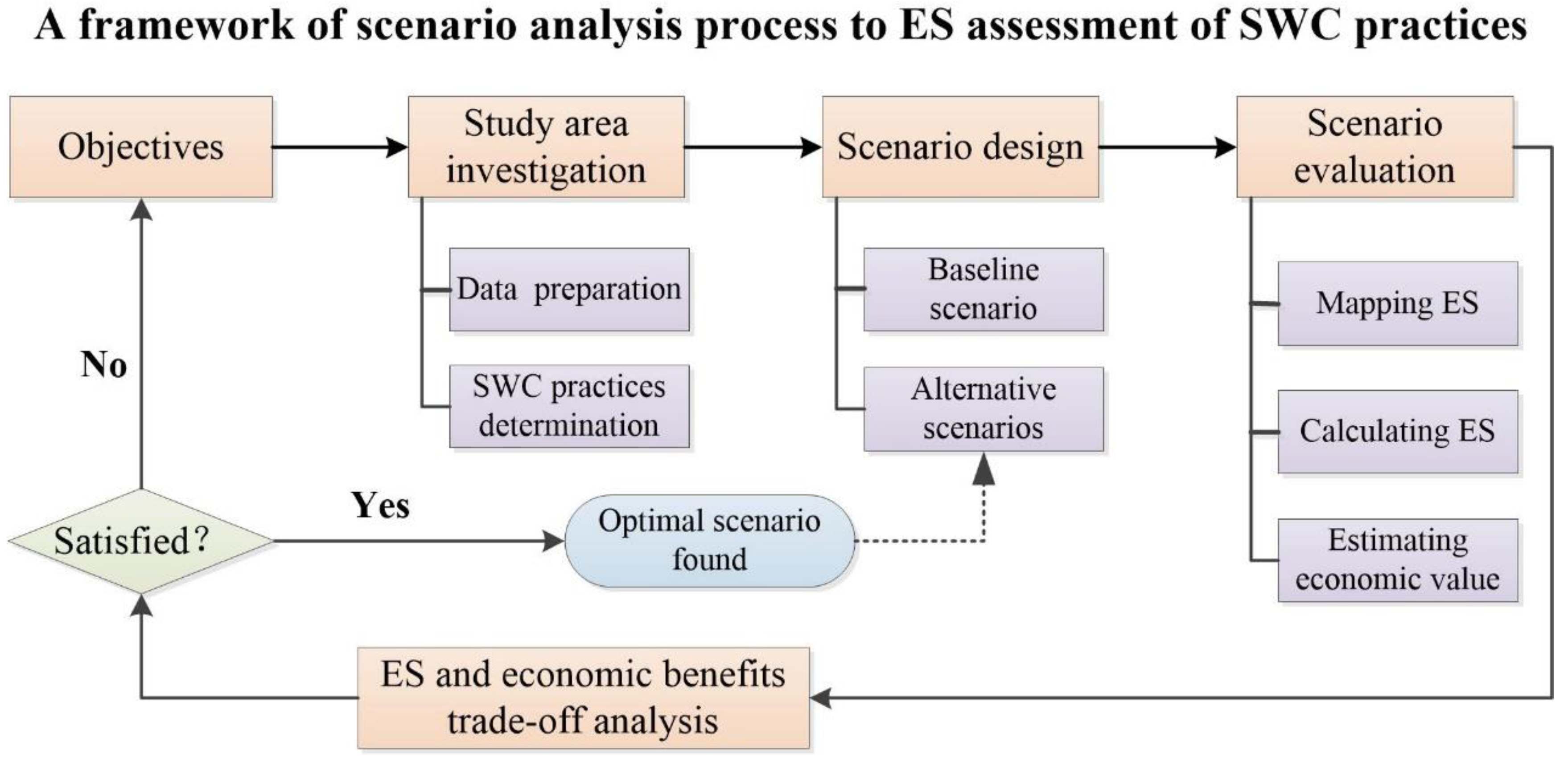
2.5. Framework of Scenario Analysis
For the scenario analysis method applied to ES assessment of SWC, they have both particularity and commonality. In this study, the particularity of the study area determines its adopted SWC practices, available data, and available methods for ES evaluation and economic benefit calculation. For example, the study area located in the hilly red-soil region of southern China determines the practices that can prevent water and soil loss and increase the income of local farmers. According to existing research, the objectives and scenario designs are also different in many studies [50]. In addition, the evaluation methods include the modelling method, indexing method, scoring method, monetization, and unified quantification, which vary directly depending on the purpose of the research [10,51].
From a more general perspective, the scenario analysis as a technology is fundamentally composed of the research objectives, research area, scenario design, scenario evaluation, and trade-off analysis. Figure 4 depicts a framework of the scenario analysis process for ES assessment of SWC practices, based on the abstraction of commonality of this research and existing research. First, research objectives need to be clear and definite, e.g., to find the optimal scenario based on ES scores and economic-benefit trade-offs in this study. Secondly, the study area investigation needs to be carried out for data preparation and the determination of SWC practices. Next, the scenarios must be designed according to the previous two steps. A baseline scenario generally adopts the current land-use status, and the alternative scenarios are designed according to the research objectives and investigation into the study area. The most important part is the scenario evaluation to quantify the ES indicators and economic costs and benefits under different scenarios. The difficulty is considering the availability of data, the rationality of ES index calculation, and the verification of model simulation. Finally, the optimal scenario is found by ES and economic-benefit trade-off analysis, and is determined by whether the research objectives are achieved. If not, it is necessary to redesign the scenario and repeat the process of the whole framework. If yes, the process ends.
3. Results and Discussion
3.1. Indicators of ES for Each Scenario
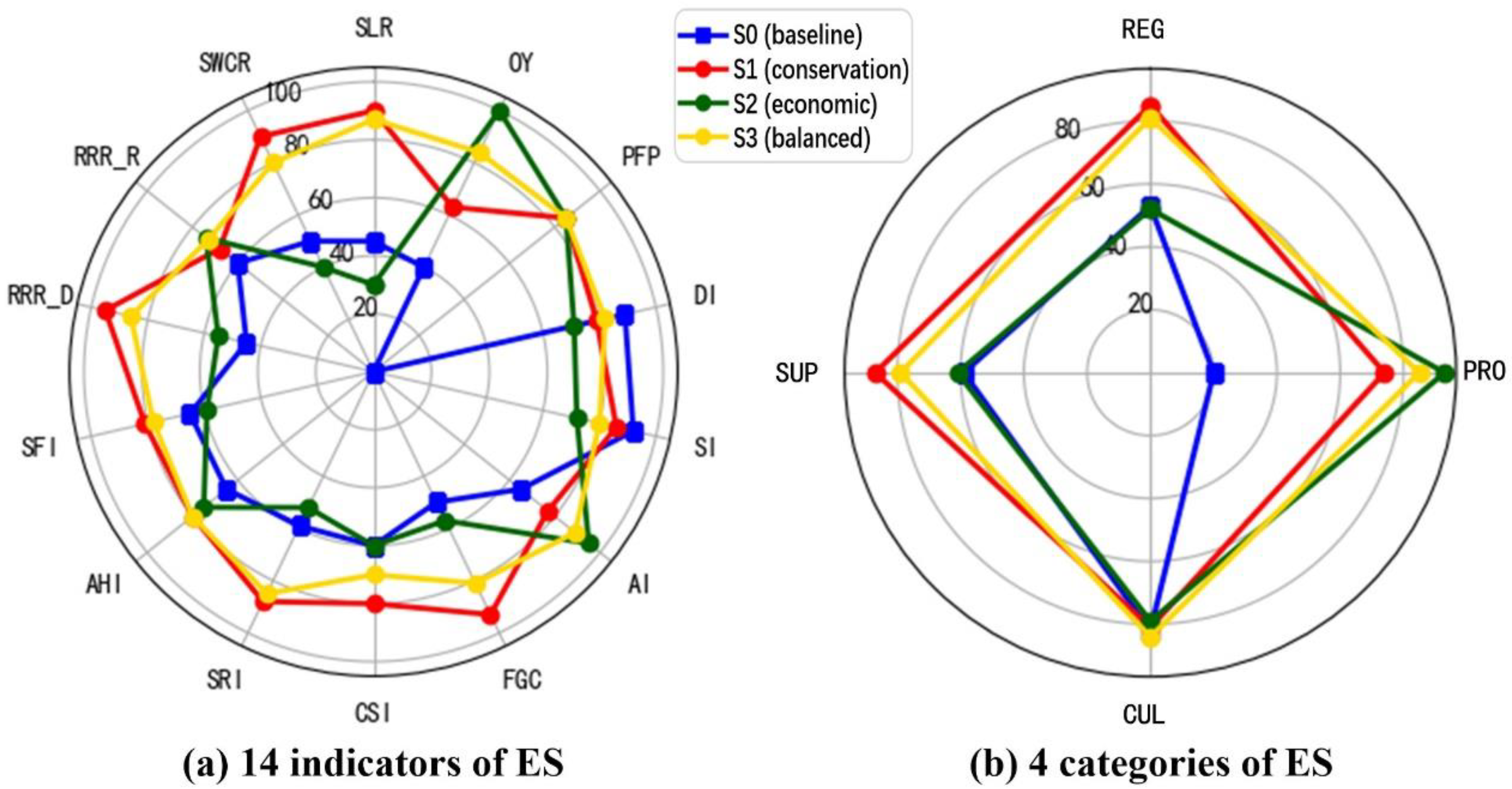
By calculating the indicators of ES for each scenario, a comparison can be performed to explore the variations in all indicators. Figure 5 depicts the scores of 14 indicators and 4 categories of ES as a whole unit in the study area. To compare S0 (baseline), the increase in most of these indicators was found in S1 (conservation) and S3 (balanced) except DI (diversity) and SI (shape) (Figure 5a). Although the scores of OY (Orchard), PFP (pond fish), and AI (area) in S2 (economic) were much higher than that in S0, the performance of other indicators was similar (Figure 5a). The seven indicators SLR (sediment), SWCR (soil conservation), RRR_D (rainy runoff), SFI (soil fertility), SRI (species richness), CSI (carbon sequestration) and FGC (forest) in S1 received top scores in all four scenarios. The three indicators OY, AI and RRR_R (dry runoff) in S3 were higher than the other three scenarios. The two indicators AHI (aquatic habitat) and PFP in S1, S2 and S3 were very close and better than in S0. Most indicators in S3 ranked second in all scenarios, which indicated that S3 was the trade-off scenario of the four scenarios.
The scores of four categories of ES calculated according to these 14 indicators are shown in Figure 5b. The REG (regulating) and SUP (supporting) in S1 were the first-rate services in all four scenarios. The scores of CUL (cultural) in all four scenarios were very close. The PRO (provisioning) in S2 increased more than that in other scenarios. The three services REG, SUP, and CUL were seen to coincide under S0 and S2, and the PRO score in S0 was the lowest of all scenarios. Most services in S3 ranked second in all scenarios (Figure 5b), which was consistent with the results of 14 indicators (Figure 5a).
3.2. Comprehensive ES Score and Economic Analysis
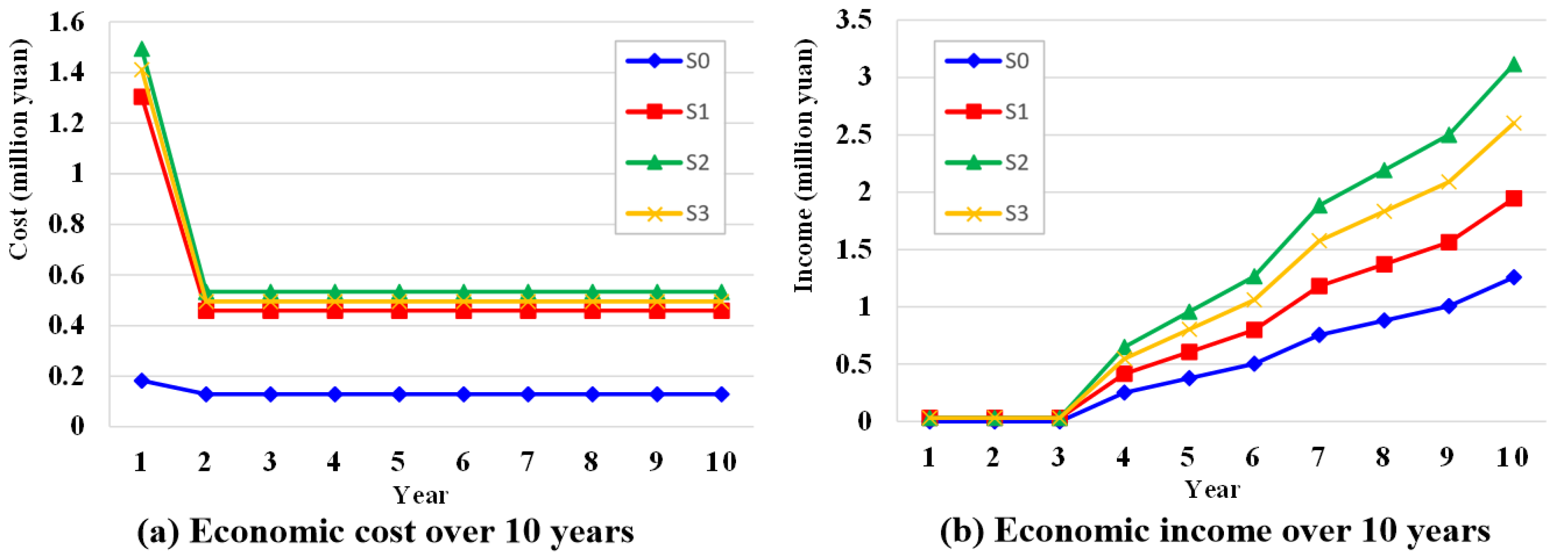
The comprehensive ES scores of all scenarios are shown in Table 7. The ES scores of S1 (conservation) and S3 (balanced) were very close, and the ranking was S3, S1, S2 (economic), and S0 (baseline). This result was consistent with the result of Figure 5. However, the ranking of the total cost over 10 years was S2, S3, S1, and S0 (Table 7). It should be indicated that while S0 had the lowest total cost, it also achieved the lowest income of all scenarios and gained the smallest ES score (53). The investment of S2 was the largest one (CNY 6.30 million), but the ES score was 71, and ranked third among the four scenarios. Excluding S2, the ES scores of other scenarios, S0, S1, and S3, raised with the increase in monetary investment. The reason might be that the cost of S2 was mainly used for the goal of economic development, while environment goals were less monetized. The highest total income over 10 years is CNY 12.66 million under S2, which might be proof of the above conjecture. The ranking of total income over 10 years was S2, S3, S1, and S0. This was consistent with the ranking of the total cost of 10 years. The ranking of net income was S2, S3, S0, and S1, different from the ranking of total income.
The concept of the income:cost ratio (N) was introduced into this study. The income:cost ratio is an indicator of economic efficiency, defined as the ratio of the income generated after the SWC practices implementation to the practices’ investment of each scenario. It has been used in many studies [52] and is similar to the concept of the input:output ratio or return on investment (ROI), which means the ratio of project input capital to output capital, that is, how many units of capital can be produced by investing one unit of capital. The greater the N, the better the economic efficiency. In Table 7, the greatest N was 3.7 under S0, while the smallest N was 1.5 under S1. The ranking of N was S0, S2, S3, and S1.
Regardless of extreme climate, market supply and demand, and other labor costs, the costs and incomes of each scenario during the 10 years are shown in Figure 6. In the beginning, the cost of all scenarios was large and fell a lot in the second year. From then on, the annual cost of each scenario remained almost the same (Figure 6a). However, the income under all scenarios showed a different performance. In the first three years, the income was very small and close to zero. From the fourth year, the income gradually increased (Figure 6b). The rank of cost and income under all scenarios was consistent with Table 6.
For the purpose of economic development, S2 (economic) was desirable because the value of the income:cost ratio (N) was relatively large. The N of S0 (baseline) was the largest, but the ES score and the total income over 10 years were the lowest. The reason might be that the traditional agricultural development has a serious impact on the environment. Under S1 (conservation), N was the smallest, but its ES score ranked second, very close to S3 (balance), the scenario of the top ES score. In fact, the economic investment of S1 brings indirect value, that is, environmental benefits, which is only reflected in the ES score, not converted into monetary value. This conclusion is consistent with the ranking of net income.
How can we choose the direct economic value or indirect environmental benefits? This involves the implicit value of environmental benefits and how to measure it. In land-use planning and policymaking, many scholars convert the value of ecological services into monetary value [8,51,53], but it is difficult to implement relevant policies because farmers with low local education cannot see the benefits of direct economic investment. With the advocacy that lucid waters and lush mountains are invaluable assets, people have begun to realize that the development of the local economy is as important as the protection of the local environment. How to choose the final scenario depends on the preferences of government decisionmakers and stakeholders. In this study, S3 (balanced) ranks second in net income (with CNY 4.73 million), preceded only by S2 (CNY 6.36 million). It might be the optimal scenario because it combines a variety of ecosystem service trade-offs, and the economic costs and benefits are balanced under different scenarios.
3.3. Discussion and Future Research
For example, S0 has no SR (small reservoir) adopted and the PFP (pond fish) is 0, which is different from the PFP under S1, S2, and S3 (Figure 5a). Another example is that the land-use diversity of S0 is greater than the other three scenarios (Figure 3), and this results in the variety of ES indicators DI (diversity), SI (shape), and AI (area) among all scenarios. The larger the patch diversity index in the landscape, the higher the DI score. The more irregular the shape, the higher the SI score. The higher the number of landscape element patches, the higher the degree of fragmentation of the landscape and the lower the AI score. However, the performance of all scenarios is similar in landscape culture service (Figure 5b). Moreover, the rank of OY (Orchard) in all scenarios is related to the area of land that adopted AST (anti-slope terrace) practice. The change in some indicators, for example, increases with the implementation area of SWC practices, or vice versa, or due to the superposition effect and interaction of practices [54], no clear trend can be determined, such as SLR (sediment), SWCR (soil conservation), SFI (soil fertility), and SRI (species richness), which needs further research in the future.
In this study, the ES indicators of runoff, soil erosion, biodiversity, soil quality, landscape culture, and fruit products were integrated, and the scenarios were evaluated according to a unified scoring mechanism. Indicators of these biophysical, social, and economic types of drivers are important for identifying the cause of the degradation and the alternative scenarios that will be part of the cost–benefit analysis (CBA) [10]. We found that the largest knowledge gap in this field is assessing the human demand for ecosystem services and the social context. The proposed cost–benefit framework of scenario analysis for ES assessment of SWC practices accompanied by ES indicators and cost–income analysis techniques enable the creation and evaluation of scenarios of alternative futures to address this gap. However, these different types of techniques are rarely combined [55], despite some ES indicators and cost–income analysis being important for the cost-effective use of land [8]. The most important lesson learned is the fact that the proposed framework should have a measure of the “human factor” included in some way to increase the applicability. However, our knowledge in these respects is unreliable and often insufficient. This paper suggests that further studies on this subject are needed.
The provision of food is a primary function and key ES of agriculture [6]. The key to poverty alleviation is to maximize the benefits of ES provision by intensive agricultural investment, which can affect ecosystem components and processes. How to balance ecological benefits and direct economic benefits is a great challenge for decisionmakers. From the income:cost ratio (N), a problem is found that is often ignored. The greater the N, the greater the grab for natural resources and the greater the damage to the ecological environment. From the perspective of sustainable development, the N of the selected scenario should not be too large, and the sustainable provision of ES needs to be considered.
The kernel idea of this study is to use ES mapping to find out the relationship between SWC practices and ES indicators and use the relationship between SWC practices and land-use change to calculate the ES score and economic cost–benefit of each scenario, to establish the methodological framework of scenario analysis for ES assessment of SWC practices. Overall, this study has the following contributions. In terms of method innovation, combined with the particularity of SWC practices in the study area, the scenarios were designed, and the localization or customization selection of ES indicators was conducted. Another contribution of this paper is that through scenario analysis, it can answer two questions. One is how much investment in SWC practices can produce how many correspondingly ecological and economic benefits. The other is what the ecological and economic trade-offs are among the different scenarios.
There are still some deficiencies in this study. First, the verification of scenario simulation results is not conducted, because the verification data onto scenario simulation are difficult to obtain. More field observations will be needed to validate how the ES impact the stakeholders. Secondly, the results of scenario evaluation (ES scores) are used for comparative analysis. The value of ES scores may be biased due to the subjective factors of ES indicators selection. However, the relative values of the four scenarios are believable for comparative analysis. In addition, a small catchment was selected as the study area without large-scale expansion in this study. However, large-scale watersheds can be divided into small catchments, and then scenario analysis for each small catchment can be performed; finally, the aggregate result can be coupled to the large watershed decision making. As a result, this method can also be used in large-scale watersheds, which plays an important role in regional high-precision and refined policymaking. Finally, the spatial computing level of ES index is not on the spatial grid scale for most of the indexes in this paper. On the one hand, it is not necessary for the purpose of this study. On the other hand, it is a great challenge for the calculation and verification on a grid scale. Much more profound research is needed in the future.
4. Conclusions
Soil erosion is quite severe in the hilly red-soil region of southern China due to the unique natural conditions, high population density, and prominent contradiction between people and land. Sustainability in the agriculture academic literature tends to incorporate ideas of the best use of environmental resources with those that are the least disruptive to these resources, leading to persistence over time and resilience [56]. To find a sustainable way for local economic development and environmental protection, this study proposes a framework of scenario analysis for the quantification analysis of ES trade-offs applied to a hilly red-soil catchment. The kernel idea of this study is mapping ES to SWC practices to find out the relationship between SWC practices and ES indicators, and then through the relationship between SWC practices and land-use change to calculate the ES scores and economic cost–benefit of each scenario, to establish the methodological framework of scenario analysis for ES assessment of SWC practices. The five SWC practices were selected for scenario design, and 14 ES indicators were used for ecosystem service assessment in this study. By calculating the ES score for all scenarios—S0 (baseline), S1 (conservation), S2 (economic), and S3 (balanced)—the results showed that S3 was the best scenario of the four scenarios. The ranking of income:cost ratio (N) was S0, S2, S3, and S1. Based on the above rankings, S3 might be the optimal scenario because it combines a variety of ecosystem services trade-offs and economic cost–benefit balance among different scenarios. The contributions of this study are the method innovation with the customization of ES indicators, and scenario analysis considering ES scores and economic-benefit trade-offs in different scenarios. However, more research is needed in the future, incorporating the “human factor”, validating the ES impact of ES on stakeholders, applying to large-scale expansion, computing ES indicators on a grid scale, and so on.
Author Contributions
Conceptualization, H.W.; methodology, L.S.; software, Z.L.; validation, H.W. and Z.L.; formal analysis, H.W.; investigation, L.S. and H.W.; resources, L.S.; data curation, H.W.; writing—original draft preparation, H.W.; writing—review and editing, H.W.; visualization, H.W.; supervision, L.S.; project administration, L.S.; funding acquisition, L.S. All authors have read and agreed to the published version of the manuscript.
Funding
This research was funded by the Natural Science Foundation of Beijing, China (Grant number 8202045), the National Key Research and Development Program of China (grant number 2017YFC050540503), the Key Research and Development Program of Zhejiang Province, China (Grant No. 2021C03138), and the National Natural Science Foundation of China (Grant number 41701520).
Institutional Review Board Statement
Not applicable.
Informed Consent Statement
Not applicable.
Acknowledgments
We appreciate ten experts for their expert knowledge. They are Fang Haiyan, at the Institute of Geographic Sciences and Natural Resources Research, Chinese Academy of Sciences; Cui Ming, at the Institute of Ecological Conservation and Restoration, Chinese Academy of Forestry; Li Zhongwu, at the School of Geographic Sciences, Hunan Normal University; Niu Xiang, at the Ecology and Nature Conservation Institute, Chinese Academy of Forest; Wei Wei, at the Research Center for Eco-Environment Sciences, Chinese Academy of Sciences; Wu Gaolin, at the Institute of Soil and Water Conservation, Northwest A&F University; Tang Zhipeng, at the Institute of Geographic Sciences and Natural Resources Research, Chinese Academy of Sciences; Zhuang Li, at the School of Environment, Jinan University; Li Chaoxia, at the College of Resources and Environment of Huazhong Agricultural University; and Xu Nan, at the Shenzhen Graduate School, Peking University. We also thank editors and reviewers for helpful conversations.
Conflicts of Interest
The authors declare no conflict of interest.
References
- Li, H.; Zhang, X.; Chen, X.; Lu, W. Soil and Water Conservation Strategies on the Red and Yellow Soils of South China. In Proceedings of the 10th International Soil Conservation Organization Meeting, West Lafayette, IN, USA, 24–29 May 1999 2001; pp. 165–170. [Google Scholar]
- Qiguo, Z. Red soils of hilly region in china: Ecological environment and strategies for integrated development. Red Lateritic Soils 1998, 2, 53. [Google Scholar]
- Wang, X. Analysis of agricultural development planning in low hilly red soil region based on planting structure. Appl. Ecol. Environ. Res. 2019, 17, 8395–8415. [Google Scholar] [CrossRef]
- Nyamekye, C.; Thiel, M.; Schönbrodt-Stitt, S.; Zoungrana, B.J.-B.; Amekudzi, L.K. Soil and water conservation in Burkina Faso, West Africa. Sustainability 2018, 10, 3182. [Google Scholar] [CrossRef] [Green Version]
- Cord, A.F.; Bartkowski, B.; Beckmann, M.; Dittrich, A.; Hermans-Neumann, K.; Kaim, A.; Lienhoop, N.; Locher-Krause, K.; Priess, J.; Schröter-Schlaack, C.; et al. Towards systematic analyses of ecosystem service trade-offs and synergies: Main concepts, methods and the road ahead. Ecosyst. Serv. 2017, 28, 264–272. [Google Scholar] [CrossRef]
- Palm, C.; Blanco-Canqui, H.; DeClerck, F.; Gatere, L.; Grace, P. Conservation agriculture and ecosystem services: An overview. Agric. Ecosyst. Environ. 2014, 187, 87–105. [Google Scholar] [CrossRef] [Green Version]
- Millennium Ecosystem Assessment. Ecosystems and Human Well-Being; Island Press: Washington, DC, USA, 2005; Volume 5. [Google Scholar]
- Farber, S.; Costanza, R.; Childers, D.L.; Erickson, J.; Gross, K.; Grove, M.; Hopkinson, C.S.; Kahn, J.; Pincetl, S.; Troy, A. Linking ecology and economics for ecosystem management. Bioscience 2006, 56, 121–133. [Google Scholar] [CrossRef] [Green Version]
- Fagerholm, N.; Torralba, M.; Burgess, P.J.; Plieninger, T. A systematic map of ecosystem services assessments around European agroforestry. Ecol. Indic. 2016, 62, 47–65. [Google Scholar] [CrossRef]
- Turner, K.G.; Anderson, S.; Gonzales-Chang, M.; Costanza, R.; Courville, S.; Dalgaard, T.; Dominati, E.; Kubiszewski, I.; Ogilvy, S.; Porfirio, L.; et al. A review of methods, data, and models to assess changes in the value of ecosystem services from land degradation and restoration. Ecol. Model. 2016, 319, 190–207. [Google Scholar] [CrossRef]
- Luo, R.; Yang, S.; Zhou, Y.; Gao, P.; Zhang, T. Spatial Pattern Analysis of a Water-Related Ecosystem Service and Evaluation of the Grassland-Carrying Capacity of the Heihe River Basin under Land Use Change. Water 2021, 13, 2658. [Google Scholar] [CrossRef]
- Costanza, R. Ecosystem services: Multiple classification systems are needed. Biol. Conserv. 2008, 141, 350–352. [Google Scholar] [CrossRef]
- Bai, Y.; Jiang, B.; Alatalo, J.M.; Zhuang, C.; Wang, X.; Cui, L.; Xu, W. Impacts of land management on ecosystem service delivery in the Baiyangdian river basin. Environ. Earth Sci. 2016, 75, 258. [Google Scholar] [CrossRef]
- Peters, M.K.; Hemp, A.; Appelhans, T.; Becker, J.N.; Behler, C.; Classen, A.; Detsch, F.; Ensslin, A.; Ferger, S.W.; Frederiksen, S.B. Climate–land-use interactions shape tropical mountain biodiversity and ecosystem functions. Nature 2019, 568, 88–92. [Google Scholar] [CrossRef] [PubMed]
- Hao, F.; Lai, X.; Ouyang, W.; Xu, Y.; Wei, X.; Song, K. Effects of land use changes on the ecosystem service values of a reclamation farm in Northeast China. Environ. Manag. 2012, 50, 888–899. [Google Scholar] [CrossRef] [PubMed]
- Metzger, M.; Rounsevell, M.; Acosta-Michlik, L.; Leemans, R.; Schröter, D. The vulnerability of ecosystem services to land use change. Agric. Ecosyst. Environ. 2006, 114, 69–85. [Google Scholar] [CrossRef]
- Fu, B.; Zhang, L.; Xu, Z.; Zhao, Y.; Wei, Y.; Skinner, D. Ecosystem services in changing land use. J. Soils Sediments 2015, 15, 833–843. [Google Scholar] [CrossRef]
- Kremen, C.; Williams, N.M.; Aizen, M.A.; Gemmill-Herren, B.; LeBuhn, G.; Minckley, R.; Packer, L.; Potts, S.G.; Roulston, T.A.; Steffan-Dewenter, I. Pollination and other ecosystem services produced by mobile organisms: A conceptual framework for the effects of land-use change. Ecol. Lett. 2007, 10, 299–314. [Google Scholar] [CrossRef]
- Liu, Y.; Li, J.; Zhang, H. An ecosystem service valuation of land use change in Taiyuan City, China. Ecol. Model. 2012, 225, 127–132. [Google Scholar] [CrossRef]
- Gachene, C.K.K.; Nyawade, S.O.; Karanja, N.N. Soil and Water Conservation: An Overview. In Zero Hunger; Leal Filho, W., Azul, A.M., Brandli, L., Özuyar, P.G., Wall, T., Eds.; Springer International Publishing: Cham, Switzerland, 2020; pp. 810–823. [Google Scholar]
- Francesconi, W.; Srinivasan, R.; Pérez-Miñana, E.; Willcock, S.P.; Quintero, M. Using the Soil and Water Assessment Tool (SWAT) to model ecosystem services: A systematic review. J. Hydrol. 2016, 535, 625–636. [Google Scholar] [CrossRef]
- Bai, Y.; Ouyang, Z.; Zheng, H.; Li, X.; Zhuang, C.; Jiang, B. Modeling soil conservation, water conservation and their tradeoffs: A case study in Beijing. J. Environ. Sci. 2012, 24, 419–426. [Google Scholar] [CrossRef]
- Tallis, H.; Polasky, S. Mapping and valuing ecosystem services as an approach for conservation and natural-resource management. Ann. N. Y. Acad. Sci. 2009, 1162, 265–283. [Google Scholar] [CrossRef]
- Liu, J.; Li, J.; Qin, K.; Zhou, Z.; Yang, X.; Li, T. Changes in land-uses and ecosystem services under multi-scenarios simulation. Sci. Total Environ. 2017, 586, 522–526. [Google Scholar] [CrossRef] [PubMed]
- Fu, Q.; Hou, Y.; Wang, B.; Bi, X.; Li, B.; Zhang, X. Scenario analysis of ecosystem service changes and interactions in a mountain-oasis-desert system: A case study in Altay Prefecture, China. Sci. Rep. 2018, 8, 12939. [Google Scholar] [CrossRef] [PubMed]
- Hu, Y.; Peng, J.; Liu, Y.; Tian, L. Integrating ecosystem services trade-offs with paddy land-to-dry land decisions: A scenario approach in Erhai Lake Basin, southwest China. Sci. Total Environ. 2018, 625, 849–860. [Google Scholar] [CrossRef] [PubMed]
- Gong, J.; Liu, D.; Zhang, J.; Xie, Y.; Cao, E.; Li, H. Tradeoffs/synergies of multiple ecosystem services based on land use simulation in a mountain-basin area, western China. Ecol. Indic. 2019, 99, 283–293. [Google Scholar] [CrossRef]
- Peng, J.; Hu, X.; Wang, X.; Meersmans, J.; Liu, Y.; Qiu, S. Simulating the impact of Grain-for-Green Programme on ecosystem services trade-offs in Northwestern Yunnan, China. Ecosyst. Serv. 2019, 39, 100998. [Google Scholar] [CrossRef]
- Schipanski, M.E.; Barbercheck, M.; Douglas, M.R.; Finney, D.M.; Haider, K.; Kaye, J.P.; Kemanian, A.R.; Mortensen, D.A.; Ryan, M.R.; Tooker, J. A framework for evaluating ecosystem services provided by cover crops in agroecosystems. Agric. Syst. 2014, 125, 12–22. [Google Scholar] [CrossRef]
- Schulte, R.P.; Creamer, R.E.; Donnellan, T.; Farrelly, N.; Fealy, R.; O’Donoghue, C.; O’huallachain, D. Functional land management: A framework for managing soil-based ecosystem services for the sustainable intensification of agriculture. Environ. Sci. Policy 2014, 38, 45–58. [Google Scholar] [CrossRef] [Green Version]
- Sun, X.; Crittenden, J.C.; Li, F.; Lu, Z.; Dou, X. Urban expansion simulation and the spatio-temporal changes of ecosystem services, a case study in Atlanta Metropolitan area, USA. Sci. Total Environ. 2018, 622, 974–987. [Google Scholar] [CrossRef]
- Sun, X.; Lu, Z.; Li, F.; Crittenden, J.C. Analyzing spatio-temporal changes and trade-offs to support the supply of multiple ecosystem services in Beijing, China. Ecol. Indic. 2018, 94, 117–129. [Google Scholar] [CrossRef]
- Power, A.G. Ecosystem services and agriculture: Tradeoffs and synergies. Philos. Trans. R. Soc. B Biol. Sci. 2010, 365, 2959–2971. [Google Scholar] [CrossRef]
- Andrew, M.E.; Wulder, M.A.; Nelson, T.A.; Coops, N.C. Spatial data, analysis approaches, and information needs for spatial ecosystem service assessments: A review. GISci. Remote Sens. 2015, 52, 344–373. [Google Scholar] [CrossRef] [Green Version]
- Hu, X.; Li, Z.; Nie, X.; Wang, D.; Huang, J.; Deng, C.; Shi, L.; Wang, L.; Ning, K. Regionalization of Soil and Water conservation Aimed at ecosystem Services improvement. Sci. Rep. 2020, 10, 3469. [Google Scholar] [CrossRef] [PubMed] [Green Version]
- Haines-Young, R.; Potschin, M. Common international classification of ecosystem services (CICES, Version 4.1). Eur. Environ. Agency 2012, 33, 107. [Google Scholar]
- Frank, S.; Fürst, C.; Koschke, L.; Witt, A.; Makeschin, F. Assessment of landscape aesthetics—Validation of a landscape metrics-based assessment by visual estimation of the scenic beauty. Ecol. Indic. 2013, 32, 222–231. [Google Scholar] [CrossRef]
- Zhu, L.-J.; Liu, J.-Z.; Qin, C.-Z.; Zhu, A.-X. A modular and parallelized watershed modeling framework. Environ. Model. Softw. 2019, 122, 104526. [Google Scholar] [CrossRef]
- Qin, C.-Z.; Gao, H.-R.; Zhu, L.-J.; Zhu, A.-X.; Liu, J.-Z.; Wu, H. Spatial optimization of watershed best management practices based on slope position units. J. Soil Water Conserv. 2018, 73, 504–517. [Google Scholar] [CrossRef] [Green Version]
- Wu, H.; Zhu, A.-X.; Liu, J.-Z.; Liu, Y.; Jiang, J. Best Management Practices Optimization at Watershed Scale: Incorporating Spatial Topology among Fields. Water Resour. Manag. 2018, 32, 155–177. [Google Scholar] [CrossRef]
- Zhu, L.-J.; Qin, C.-Z.; Zhu, A.-X.; Liu, J.-Z.; Wu, H. Effects of different spatial configuration units for the spatial optimization of watershed best management practice scenarios. Water 2019, 11, 262. [Google Scholar] [CrossRef] [Green Version]
- Vaidya, O.S.; Kumar, S. Analytic hierarchy process: An overview of applications. Eur. J. Oper. Res. 2006, 169, 1–29. [Google Scholar] [CrossRef]
- Saaty, T.L. Decision making with the analytic hierarchy process. Int. J. Serv. Sci. 2008, 1, 83–98. [Google Scholar] [CrossRef] [Green Version]
- Tian, J.; Guo, S.; Deng, L.; Yin, J.; Pan, Z.; He, S.; Li, Q. Adaptive optimal allocation of water resources response to future water availability and water demand in the Han River basin, China. Sci. Rep. 2021, 11, 7879. [Google Scholar] [CrossRef] [PubMed]
- Wang, X.; Zhang, X.; Guo, X. Spatial-Temporal variation of soil fertility quality of Jiangxi province in the past 30 years. Jiangsu Agric. Sci. 2018, 46, 284–288. (In Chinese) [Google Scholar]
- Wang, J.; Tian, J.; Lu, X. Assessment of stream habitat quality in Naoli River Watershed, China. Acta Ecol. Sin. 2010, 20, 481–486. (In Chinese) [Google Scholar]
- Spellerberg, I.F. Shannon–Wiener Index. In Encyclopedia of Ecology; Jørgensen, S.E., Fath, B.D., Eds.; Academic Press: Oxford, UK, 2008; pp. 3249–3252. [Google Scholar]
- Sharp, R.; Tallis, H.; Ricketts, T.; Guerry, A.; Wood, S.A.; Chaplin-Kramer, R.; Nelson, E.; Ennaanay, D.; Wolny, S.; Olwero, N. InVEST User’s Guide; The Natural Capital Project: Stanford, CA, USA, 2014. [Google Scholar]
- McGarigal, K. FRAGSTATS: Spatial Pattern Analysis Program for Quantifying Landscape Structure; US Department of Agriculture, Forest Service, Pacific Northwest Research Station: Portland, OR, USA, 1995; Volume 351.
- Kishita, Y.; Hara, K.; Uwasu, M.; Umeda, Y. Research needs and challenges faced in supporting scenario design in sustainability science: A literature review. Sustain. Sci. 2016, 11, 331–347. [Google Scholar] [CrossRef]
- Momblanch, A.; Connor, J.D.; Crossman, N.D.; Paredes-Arquiola, J.; Andreu, J. Using ecosystem services to represent the environment in hydro-economic models. J. Hydrol. 2016, 538, 293–303. [Google Scholar] [CrossRef]
- Cardozo, E.G.; Muchavisoy, H.M.; Silva, H.R.; Zelarayán, M.L.C.; Leite, M.F.A.; Rousseau, G.X.; Gehring, C. Species richness increases income in agroforestry systems of east-ern Amazonia. Agrofor. Syst. 2015, 89, 901–916. [Google Scholar] [CrossRef]
- Losey, J.E.; Vaughan, M. The economic value of ecological services provided by insects. Bioscience 2006, 56, 311–323. [Google Scholar] [CrossRef] [Green Version]
- Lal, R. Soil conservation and ecosystem services. Int. Soil Water Conserv. Res. 2014, 2, 36–47. [Google Scholar] [CrossRef] [Green Version]
- Dunford, R.; Harrison, P.; Smith, A.; Dick, J.; Barton, D.N.; Martin-Lopez, B.; Kelemen, E.; Jacobs, S.; Saarikoski, H.; Turkelboom, F. Integrating methods for ecosystem service assessment: Experiences from real world situations. Ecosyst. Serv. 2018, 29, 499–514. [Google Scholar] [CrossRef] [Green Version]
- Sherman, J.; Gent, D.H. Concepts of sustainability, motivations for pest management ap-proaches, and implications for communicating change. Plant Dis. 2014, 98, 1024–1035. [Google Scholar] [CrossRef] [Green Version]
Figure 1.
The location of the study area and maps of DEM, land use, and soil types. (a) The location of the study area, in Jiangxi Province, China. (b) The DEM of the study area. (c) The land-use types of the study area. (d) The soil types of the study area.
Figure 1.
The location of the study area and maps of DEM, land use, and soil types. (a) The location of the study area, in Jiangxi Province, China. (b) The DEM of the study area. (c) The land-use types of the study area. (d) The soil types of the study area.

Figure 2.
The monthly average precipitation from 2018 to 2016.

Figure 3.
The placements of SWC practices of baseline scenario and alternative scenarios. (a) The distribution of land-use types in S0 (baseline). (b) The distribution of SWC practices in S1 (conservation). (c) The distribution of SWC practices in S2 (economic). (d) The distribution of SWC practices in S3 (balanced).

Figure 4.
A framework of scenario analysis process for ES assessment of SWC practices.

Figure 5.
The scores of 14 indicators and 4 categories of ES. (a) The scores of 14 indicators in all scenarios. (b) The scores of 4 categories in all scenarios.
Figure 5.
The scores of 14 indicators and 4 categories of ES. (a) The scores of 14 indicators in all scenarios. (b) The scores of 4 categories in all scenarios.

Figure 6.
The economic cost and income over 10 years for all scenarios. (a) The economic cost over 10 years for all scenarios. (b) The economic income over 10 years for all scenarios.
Figure 6.
The economic cost and income over 10 years for all scenarios. (a) The economic cost over 10 years for all scenarios. (b) The economic income over 10 years for all scenarios.

Table 1.
Detailed description of the data.
| Data Name | Description | Data Source |
|---|---|---|
| Precipitation | Time serial, daily | REDCP, http://www.resdc.cn (accessed on 26 February 2022) |
| DEM | Grid size: 30 m and 2 m | REDCP and data of UAV |
| Land use | Grid size: 30 m and 2 m | REDCP and data of UAV |
| Soil type | Grid size: 30 m | Harmonized World Soil Database |
| Soil properties | Soil particle size, total nitrogen, total phosphorus, total potassium and organic matter in soil | Laboratory measurements |
| Local species | Number of species and population of each specie in ecosystem | Field investigations |
| Hydrologic characteristics | Runoff and sediment records, time serial, daily | Hydrologic yearbook |
Table 3.
The indicators of ES and associated soil and water conservation practices.
| ID | Indicators of ES | Associated Soil and Water Conservation Practices | Categories of ES |
|---|---|---|---|
| 1 | Sediment loss rate | AST, CHM, BF, HCD | Regulating service (REG) |
| 2 | Soil and water conservation rate | AST, CHM, BF, HCD | |
| 3 | Runoff regulation rate in rainy season | AST, CHM, BF, HCD | |
| 4 | Runoff regulation rate in dry season | AST, CHM, BF, HCD | |
| 5 | Soil fertility index | AST, CHM, HCD | |
| 6 | Aquatic habitat index | SR, BF | Supporting service (SUP) |
| 7 | Species richness index | CHM, BF, HCD | |
| 8 | Carbon sequestration index | AST, CHM, BF, HCD | |
| 9 | Forest and grass coverage | CHM, BF | |
| 10 | Area index | AST, CHM, BF, HCD, SR | Cultural service (CUL) |
| 11 | Shape index | AST, CHM, BF, HCD, SR | |
| 12 | Diversity index | AST, CHM, BF, HCD, SR | |
| 13 | Pond culture yield | SR | Provisioning service (PRO) |
| 14 | Orchard yield | AST |
Table 5.
The cost of investment for soil and water conservation practices (CNY/ha).
| Practices ID | Cost of One-Time Investment | Cost of Annual Investment |
|---|---|---|
| 1 for AST | Terrace land preparation cost and fruit tree | Grass planting cost and fertilization cost |
| 2 for SR | Small reservoir construction cost | Fish fry cost |
| 3 for CHM | Seedling cost | Replant Seedling cost |
| 4 for BF | Seedling cost | Replant Seedling cost |
| 5 for HCD | Ditch excavation cost | Hedgerow planting cost |
Table 6.
The income of navel oranges over 10 years (CNY 10,000/ha).
| Year | 1 | 2 | 3 | 4 | 5 | 6 | 7 | 8 | 9 | 10 |
|---|---|---|---|---|---|---|---|---|---|---|
| Income | 0 | 0 | 0 | 5 | 7.4 | 9.9 | 14.9 | 17.3 | 19.8 | 24.8 |
Table 7.
The ES scores and economic data over 10 years among the four scenarios.
| Scenarios | S0 (Baseline) | S1 (Conservation) | S2 (Economic) | S3 (Balanced) |
|---|---|---|---|---|
| ES scores | 53 | 81 | 71 | 82 |
| Total cost over 10 years (million CNY) | 1.35 | 5.44 | 6.30 | 5.87 |
| Total income over 10 years (million CNY) | 5.03 | 7.98 | 12.66 | 10.60 |
| Net income over 10 years (million CNY) | 3.68 | 2.54 | 6.36 | 4.73 |
| Income:cost ratio, (N) | N = 3.7 | N = 1.5 | N = 2.0 | N = 1.8 |
Publisher’s Note: MDPI stays neutral with regard to jurisdictional claims in published maps and institutional affiliations. |
© 2022 by the authors. Licensee MDPI, Basel, Switzerland. This article is an open access article distributed under the terms and conditions of the Creative Commons Attribution (CC BY) license (https://creativecommons.org/licenses/by/4.0/).
Share and Cite
MDPI and ACS Style
Wu, H.; Sun, L.; Liu, Z. Ecosystem Service Assessment of Soil and Water Conservation Based on Scenario Analysis in a Hilly Red-Soil Catchment of Southern China. Water 2022, 14, 1284. https://doi.org/10.3390/w14081284
AMA Style
Wu H, Sun L, Liu Z. Ecosystem Service Assessment of Soil and Water Conservation Based on Scenario Analysis in a Hilly Red-Soil Catchment of Southern China. Water. 2022; 14(8):1284. https://doi.org/10.3390/w14081284
Chicago/Turabian StyleWu, Hui, Liying Sun, and Zhe Liu. 2022. "Ecosystem Service Assessment of Soil and Water Conservation Based on Scenario Analysis in a Hilly Red-Soil Catchment of Southern China" Water 14, no. 8: 1284. https://doi.org/10.3390/w14081284
Note that from the first issue of 2016, this journal uses article numbers instead of page numbers. See further details here.