Water Flow Characteristics Controlled by Slope Morphology under Different Rainfall Capacities and Its Implications for Slope Failure Patterns

Abstract

The high sensitivity of loess slopes to water has been emphasized in many studies. However, it is still limited in terms of the understanding of slope morphological differentiation on the overall and local failure patterns in slopes, as well as on the acquisition method of hydrological dynamics. In this study, rainfall characteristics and slope surface morphological differences were introduced. Geoelectric and environmental factors were monitored. On this basis, apparent resistivity corrected by seasonal temperature and its relationship with soil water content was calibrated. The water migration characteristics and potential failure patterns of three slope morphologies were evaluated. The results are: (i) the improved resistivity method can better reflect the water flow movement within the slope, and it performs well after being corrected by temperature; (ii) the characteristics of surface runoff and water infiltration are directly affected by the cumulative rainfall value, and especially when the cumulative rainfall is >70 mm threshold, the surface runoff quickly infiltrates into the deep of the slope along the preferential paths; (iii) the interception ability of loess slope morphology to the surface runoff is concave slope > convex slope > linear slope; (iv) with the continuous rainfall, the convex surface of a slope is prone to be damaged by saturated mud flow. When the cumulative rainfall threshold is 70 mm, the preferential flow is easily excited on the concave surface of the slope, resulting in local collapse at the slope toe and mid-deep landslides.

1. Introduction

In recent years, more and more attention has been paid to the sustainable development of surface environment [1]. Research on the changes of surface environment plays an important role in the stability and sustainable development of human settlements and geological environment in an area, especially in terms of changes in surface morphological characteristics, which sometimes affect people′s production and life [2]. As a kind of surface morphology, loess slope morphology is widely distributed in the Chinese Loess Plateau. It can be divided into concave slope, convex slope, linear slope and stepped slope according to the morphological differences [3,4]. When the sensitivity of loess to water is considered [5], the slope morphology is linked with the study of soil and water conservation. It can provide a basis for taking engineering measures for soil erosion [6,7]. In addition, the difference of slope morphology affects the redistribution of rainfall. It further controls the occurrence of surface runoff and water migration within the slope body and promotes the further development of potential slope failure [1]. This phenomenon occurs in the slope landscape of the Chinese Loess Plateau from time to time. It includes natural slope and fill slope. Therefore, in the context of rainfall, surface–underground water migration occurs, and the difference of slope morphological characteristics leads to the development of potential slope failure [8]. How to properly describe these laws and mechanisms is important. It can provide support for the technical method system of territorial space ecological restoration in the new era of national land space ecological restoration in the new era of China.

In order to understand the correlation between surface–underground hydrological dynamics and slope failure pattern and slope morphology under rainfall behavior, the methods such as numerical simulation and physical model experiment have been adopted and practiced by scholars, and these approaches have made some progress [1,9]. However, the accuracy of a numerical simulation depends on the simulation parameters. Due to the change of boundary conditions, some simulation parameters are difficult to obtain. The numerical simulation results still deviate from the actual situation. In addition, artificial rainfall is applied, and the physical model easily controls the slope surface morphology, which is convenient for the following research: (i) correlation between soil erosion and slope angle; (ii) correlation between surface runoff and slope surface morphology; (iii) the role of slope surface morphology in revealing the process of underground water migration; (iv) the influence of slope surface morphology on the failure mechanism of slope body [7,10]. However, experiments are expensive and have some restrictive factors. For example, it is impossible to present the real soil structure within the natural slope. In order to solve this problem, field monitoring has been given increasing attention. For example, through site investigation, the typical morphology slope is selected for in situ field monitoring. It can be used to study the interception effect of slope morphology on surface runoff, the water migration and the potential failure within the slope in the process of long-term rainfall.

There are many field monitoring methods. For example, the weight method is simple to operate and has sufficient accuracy. However, it is time-consuming and laborious, and is not suitable for continuous and dynamic monitoring of soil moisture at fixed points. The neutron probe method does not need to destroy the soil structure. It can obtain the law of soil water migration at the sampling point. However, the vertical resolution of the neutron probe is very low. It is expensive and its radiation is harmful to health. The time-domain reflectometry (TDR) method has the advantages of high time resolution, fast acquisition speed and repeatability of measurement. However, the cost of its large-scale deployment for monitoring is high [11]. In order to solve the above disadvantages, a new method is needed for slope monitoring. Geophysical methods such as electrical resistivity tomography as a way of field monitoring [12] not only have the characteristics of minimal invasiveness, repeatability and sensitivity to water, but also have the functions of automatic frequency modulation, automatic collection and automatic data transmission by connecting to the internet. Therefore, they are widely used in the monitoring of slope hydrological changes during rainfall [13]. For example, when electrical resistivity tomography is used for long-term monitoring of slope hydrology, the difference between effective porosity and water content can be used to assess the lack of soil water content in slope runoff [14], and the relationship between the increase in underground water content of shallow landslides and the failure event can be found [15]. In addition, the preferential pathways on the water infiltration process can also be characterized on the local scale [16,17]. Hence, electrical resistivity tomography is used for field monitoring, which can capture the large-area information of soil water content change in the rainfall process within the slope [18]. By shortening the collection time, electrical resistivity tomography images can show a more continuous water migration process. They can be used to study the surface–underground water migration of different slope morphologies on the same slope.

However, there are still some challenges. For example, one challenge is how to divide rainfall characteristics reasonably in order to provide key rainfall information for studying the water characteristics of a morphological slope [19]. When the climate and season change, they can affect the soil water content within the loess slope. This can also cause fluctuations in underground temperature, which affects electrical resistivity tomography geoelectric monitoring results [15]. Hence, how to eliminate the temperature interference to track the high-resolution water migration process is a problem to be solved. In addition, the difference of slope surface morphology affects the surface runoff. This difference is generally presented in the form of relationship curves, which are plotted by software simulation or field measurement data [7]. Especially in the process of rainfall, surface runoff and groundwater migration are closely related. However, few studies have mentioned the above systematic considerations to monitor the impact of slope morphological differentiation on local or overall water acquisition and potential slope failure patterns through electrical resistivity tomography.

This paper aims to present water flow characteristics controlled by slope morphology under different rainfall capacities and its implications for slope failure patterns. It provides support for in-depth understanding of the influence of slope morphological differentiation on obtaining local slope hydrological dynamics and potential failure patterns. It also provides an understanding of the method of slope global hydrological acquisition. In this context, the experimental site was selected, and the in situ data of geoelectric and environmental parameters such as soil temperature and soil water content were monitored. Variation trends of overall apparent resistivity of the slope under six rainfall scenarios were evaluated. The results of the resistivity field, soil water content field and soil water content ratio field of three slope morphologies considering environmental factors under six rainfall scenarios are presented. The intercepting ability of surface runoff and the potential failure patterns for three slope morphologies are discussed. The research results are then summarized.

2. Materials and Methods

2.1. Site Description

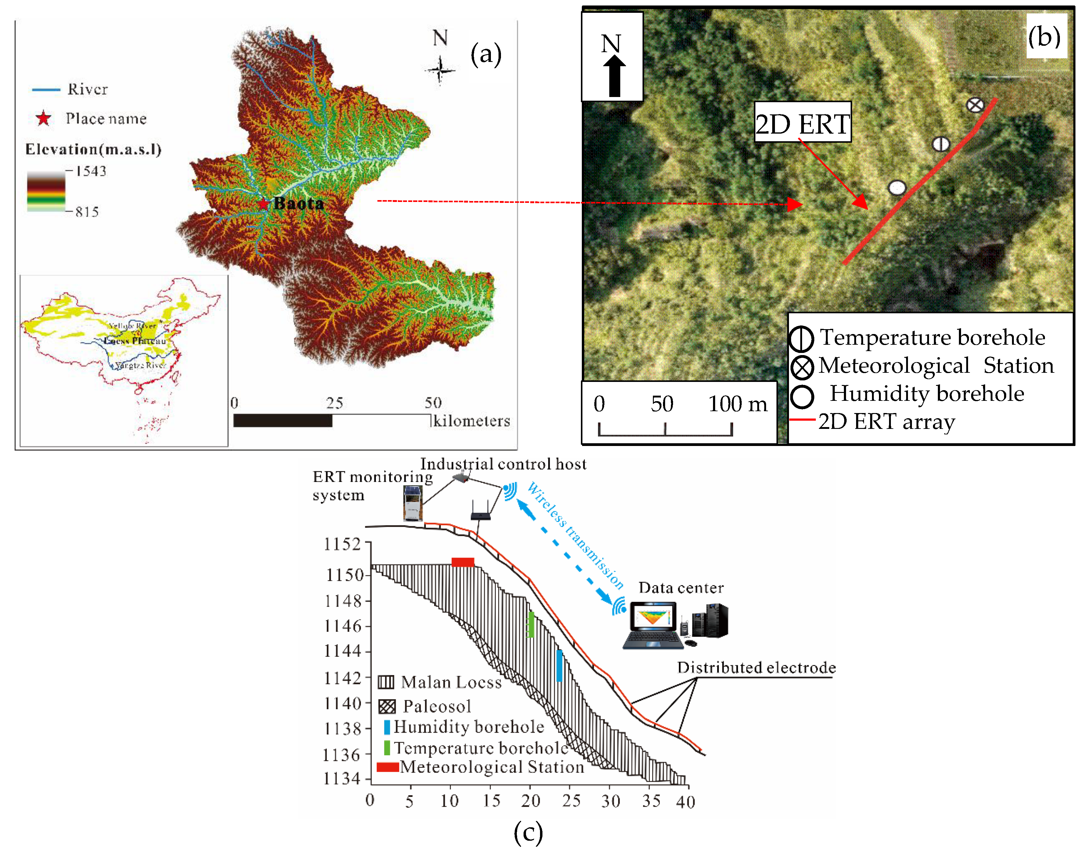
The study site is located in the Baota District, Yan′ an, which covers 3556 km² and is located between 109°14′–110°07′ E and 36°11′–37°02′ N (Figure 1a). The topography of the study area is characterized by the intertwined terrain of hills and gullies, with an altitude of 700~1400 m. The area is covered with thick Pleistocene loess. It includes early Pleistocene Malan loess (Q₃) with a thickness of about 10–30 m, Middle Pleistocene Lishi loess (Q₂) and late Pleistocene Wucheng loess (Q₁) [3,4]. In addition, the annual temperature in the area varies between −5 °C and 23 °C, with an average temperature of 10.4 °C. Rainfall mainly occurs from June to September, accounting for 60–80% of the annual rainfall. The distribution of rainfall is uneven. It can be seen clearly in the dry season and rainy season. Thunderstorms are mainly in summer and continuous cloudy rain is mainly in autumn. It is easy to cause geological disasters such as loess landslides in the study area. For example, in July 2013, there was heavy rain in the Yan′an area. The rainwater infiltrated into the slope along the preferential pathways [17], which increased the hydrodynamic pressure of the slope and caused the instability of some slopes [9]. At the same time, the continuous rainfall caused mudflows on slope surface in the large areas. These mudflows blocked many roads, destroyed lots of cave dwellings and caused several deaths [4]. The loess mudflow phenomenon is common in the Yan′an area. According to the geological hazard survey data of Baota District in the Yan′an, there were 16 recorded mudflow disasters in the Baota District in the five years from 2001 to 2005. It caused 2 deaths and CNY 300,000 economic loss. Therefore, frequent slope mudflow damage events brought serious impact on the safety of lives and property and normal production and life of the local people.

The Pijiagou slope was used as the test site, which is near the meteorological station in the Baota District (Figure 1b). The strike of the slope is northwest–southeast, with the length of nearly 90 m and the height of nearly 20 m. In addition, the slope fluctuates greatly; the average slope angle is close to 22°. The slope angle varies greatly at different locations, ranging from 0° to 50°. However, it presents different slope morphology. The sides of the slope and the platform are mainly covered with weeds. Meanwhile, some tensile cracks, fissures and animal and plant holes are distributed on the slope. Under heavy rain conditions, it is easy to cause preferential infiltration phenomena. Hence, the 2D electrical resistivity tomography equipment is deployed on the slope for long-term monitoring of the slope hydrological environment under different rainfall events. It can not only reveal water flow characteristics controlled by slope morphology under different rainfall characteristics, but also provide necessary data for studying the implicated failure patterns during the rainfall process.

2.2. Field Installation

The measurement system used for data monitoring includes apparent resistivity measuring equipment, temperature sensor, soil moisture sensor and meteorological station (Figure 1c). The apparent resistivity measurement equipment is electrical resistivity tomography monitoring equipment improved by Sun [20], which includes electrodes, converters, remote automatic monitoring system, industrial control host, wireless transmission system and computer terminal. The equipment has the advantages of unattended, automatic data measurement and remote transmission, which greatly improves the collection efficiency and can realize long-term observations of slope apparent resistivity.

Based on the above electrical resistivity tomography system configuration, through site survey, the potential sliding direction of the Pijiagou slope was approximately laid out with a 40 m long 2D electrical resistivity tomography measuring line. Eighty electrodes were connected to the survey line at electrode spacing of 0.5 m, and eight electrodes were used as a group, which was controlled by a converter. Finally, each converter connected in series with each other was integrated into the remote automatic monitoring system, and then connected with the industrial control host. Through the wireless transmission system, they linked with the data center to form a long-term in situ apparent resistivity acquisition system. The acquisition system realized remote monitoring of the slope, eliminated the dependence on repeated monitoring access and improved the time resolution of apparent resistivity acquisition [20].

In addition, a temperature borehole and humidity borehole were dug near the 2D electrical resistivity tomography line to install temperature sensors and soil moisture sensors and supplemented by the meteorological station to collect surface air temperature and rainfall data. The temperature sensor with HSTL-102STRWS model was composed of precision platinum resistance and high-precision transmitter. The transmitter was composed of power module, temperature sensing module, transmission module, temperature compensation module and data processing module. The transmitter had zero drift circuit and temperature compensation circuit, which had high applicability to the environment. A variety of data collectors with differential input, data acquisition card, remote data acquisition module and other equipment were connected to the temperature sensor. In the range of 0 to 50 °C, the relationship T = 3.125A − 12.5 can be used to convert each collected current into temperature value.

The soil moisture sensor with model HS-102STR is a high-sensitivity sensor that measures soil moisture based on the principle of frequency domain reflection. By measuring the soil dielectric constant, it can directly and stably reflect the real soil moisture content. The measurement accuracy is ±2%. In addition, the linear relationship of θ_v = 27.573 V − 0.3217 within the range of saturated soil moisture content was obeyed. Where 0 ≤ θ_v ≤ 50%, θ_v is soil volumetric content, V is the voltage measured by the collector.

The meteorological station was used to collect surface air temperature and rainfall data. The rainfall data were collected by a single bucket current-type rain gauge, with the diameter of 200 mm, the measurement range of ≤8 mm/min, the resolution of 0.2 mm, the error of ±2% and the working environment temperature of 20 °C ± 30 °C for collection. The surface temperature was measured by a JXBS-3001-TH air temperature transmitter, the measurement range was −20 to 60 °C, the resolution was 0.1 °C, the error was ±0.3 °C and the long-term stability of temperature can be maintained at ≤0.1 °C/yr. The monitoring period was from 24 June 2017 to 28 January 2018, which experienced summer, autumn and winter.

2.3. Data Collection and Analysis

2.3.1. Apparent Resistivity Acquisition

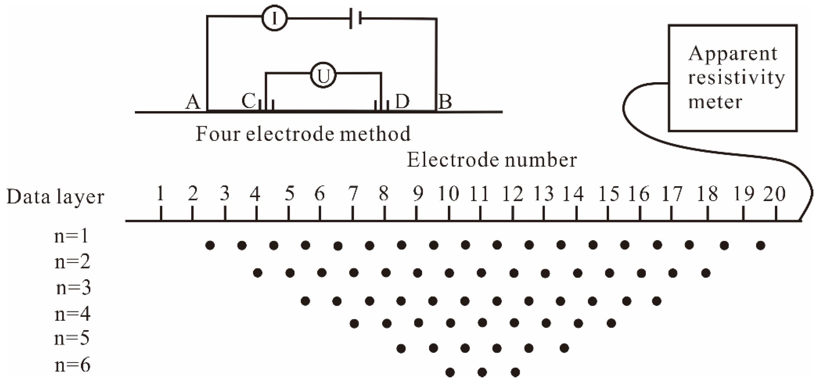
The apparent resistivity data acquisition involves the current injection between two electrodes and the measurement of the potential difference between the other electrodes. As shown in Figure 2, the current I is injected into the loess medium through a pair of current electrodes (A, B), and the voltage U is measured between the second pair of potential electrodes (C, D). Apparent resistivity ρ_s (Ωm) on semi-infinite, inhomogeneous, isotropic media can be expressed as [21]:

$${\rho }_s=2\pi KU/I$$

(1)

where K is the geometric factor, which depends on the electrode arrangement. Wenner arrangement (A, C D, B) was used for the acquisition of apparent resistivity, and the electrode spacing was equal. The data were collected by the apparent resistivity meter each time through multiple tests. It was transmitted to the computer through the remote automatic monitoring system, industrial control host and wireless transmission system, which was convenient for researchers to process and analyze (Figure 1b,c).

Relying on the survey lines laid out on the slope, the apparent resistivity acquisition equipment began to work normally on 25 June 2017, with the maximum acquisition frequency for 4 times per day. As of 10 December 2017, 624 groups of apparent resistivity were collected. According to the required data, the data including the six rainfall scene periods were selected for research. It was from 15 July 2017 to 10 December 2017.

2.3.2. Apparent Resistivity Processing

After the raw data of apparent resistivity are collected each time, they are used for inversion through res2dinv commercial software [22]. Before that, pretreatment is required. For example, the abrupt resistance values are removed. The limited range of model resistivity value is set between 50–350 ohms, which is consistent with the distribution range of loess resistivity in the study area. Then, the iterative optimization algorithm based on least square smoothing constraint is used as the inversion scheme [23,24]. In this context, the underground space is divided into many model sub-blocks through the two-dimensional model in the inversion program. Then, the resistivity of these sub-blocks is determined, so that the forward calculated apparent resistivity pseudo section is consistent with the measured pseudo fault value. The optimization method is that the resistivity of the model sub-block is adjusted to reduce the difference between the forward value and the measured apparent resistivity. This difference is measured by mean square error [25]. Based on this, the apparent resistivity is inversed into resistivity, which can then be corrected by temperature in turn to study the change of resistivity in the process of rainfall.

2.3.3. The Relationship between Apparent Resistivity and Soil Water Content

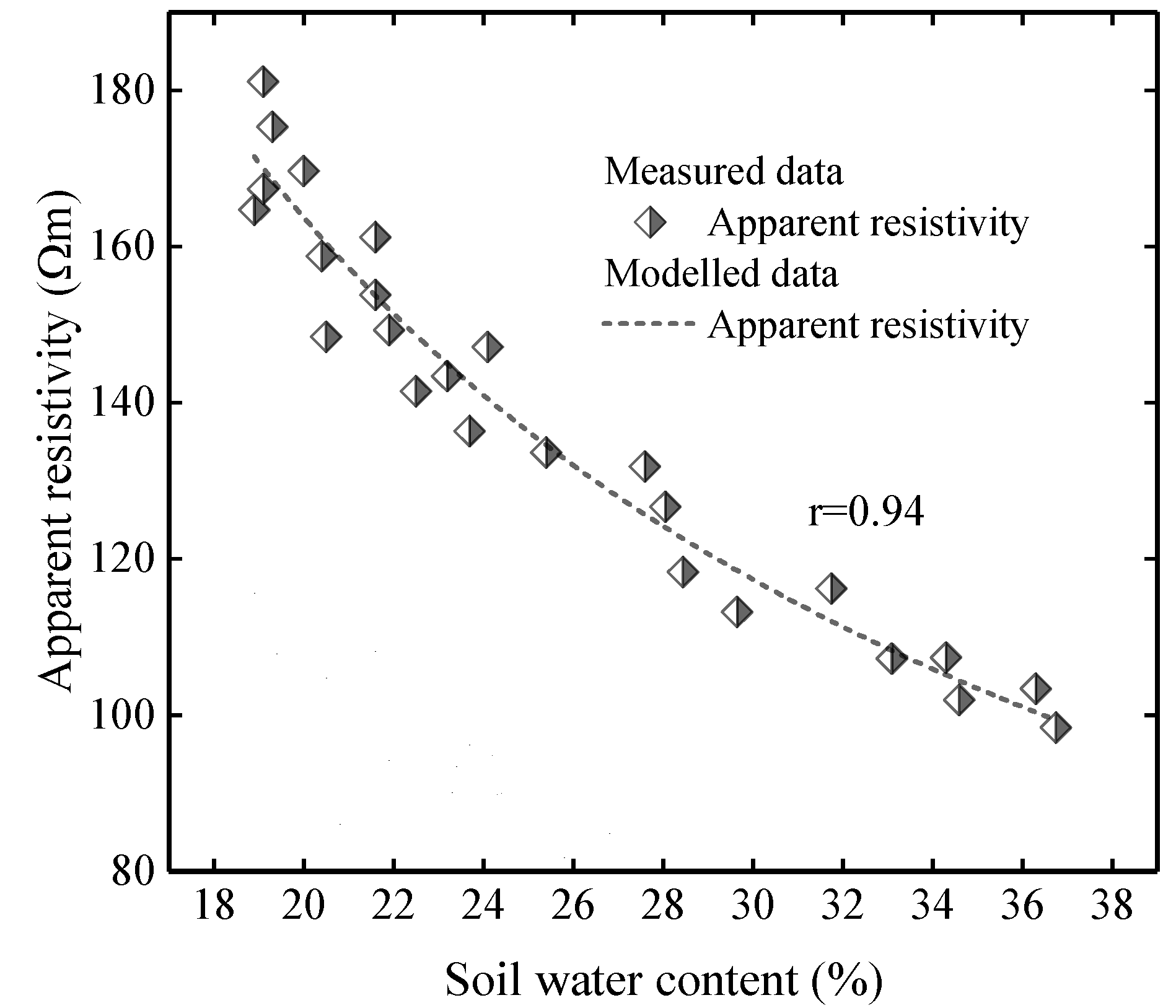
Water plays a key role in current conduction in loess. Hence, it is necessary to obtain the soil moisture content, which can be measured by using the soil moisture sensor connected to the automatic measurement system. The collected soil water content and apparent resistivity at the same time and at the same depth are characterized by Archie′s equation [26], and the relationship is as follows:

$${\rho }_s=a{\varphi }^{n-m}{\theta }^{-n}{\rho }_w$$

(2)

where ρ_s is the bulk apparent resistivity; ρ_w is apparent resistivity of the loess pores; ϕ is the porosity; θ is the soil water content; m is the cementation index; n is the saturation coefficient; a is the constant [27]. It assumes that the apparent resistivity of the loess properties and pore-water of an entire slope are homogeneous, then aϕ^n−mρ_w could be replaced with the constant A, and the Equation (2) is rewritten as:

$${\rho }_s=A{\theta }^{-n}$$

(3)

Based on the model (A = 3801, n = 1.18, R = 0.95) relationship between apparent resistivity and soil water content, a set of best fitting models can be obtained through two parameters. The calibrated model is shown in Figure 3. In addition, the slope morphology affects the flow and infiltration of rainwater. The result of this influence can be judged by the average water content of different slope morphology areas during the rainfall. In fact, it implies the interception ability of different slope morphologies to surface runoff. In this context, the monitored resistivity can be converted into soil water content through Equation (3). It is used as the basic data to evaluate the interception ability of different slope morphologies to surface runoff.

2.3.4. Temperature Model Correction

The resistivity in the loess soil is highly sensitive to temperature change. The resistivity above 0 °C linearly decreases by about 2%/°C with the increase of temperature [28]. Changes in formation resistivity are caused by seasonal temperature changes, which are even of the same magnitude as those caused by hydrological processes. After the apparent resistivity is inversed into resistivity, it needs to be corrected by the standard temperature to eliminate these seasonal changes and avoid misunderstandings of the resistivity monitoring data [23].

Therefore, temperature data of 0.6 m, 1.0 m, 1.5 m and 2.0 m depths in the borehole within one year were recorded. On this basis, the model of Brunet [14] was modified (Equation (4)), and the simplified temperature model suitable for seasonal variation of loess in this area was established to evaluate the seasonal variation of underground temperature. Part temperature model parameters are shown in

Table 1. Part temperature model parameters of Equation (4).

Depth (m)	Z	d	f
0.6	0.6	0.6	14.3
1	1	0.5	13.3
1.5	1.5	0.5	12.4
2	2	0.5	12.8

z is the depth below the surface. The temperature sensors are installed at these depths for long-term monitoring of ground temperature; d is a depth parameter of the model; f is the phase shift.

.

$$T(z,t)=T_{mean}(air)+T_p+A{e}^{-(z/d)}\sin (wt+f-z/d)$$

(4)

where T(z, t) is the temperature on day t and at depth z; T_mean is the annual average temperature; T_p is the correction coefficient, and its value is 3.0 °C; A is the annual variation of temperature; d is a depth parameter of the model; f is the phase shift, and the constant phase shift can ensure that the surface temperature is synchronized with the air temperature; (f − z/d) is the phase lag; the frequency of the periodic change P is ω (ω = 2π/P, where p = 365 days). From the temperature recorded over the years in the area, T_mean = 10.4 °C, A = 14.6 °C were obtained. The model was successfully applied at the depths of 0.6 m, 1.0 m, 1.5 m and 2.0 m. It was found that the deviation between the calculated model temperature and the actual temperature is no more than 2%. It may be assumed that when the depth exceeded 2.0 m, the difference between the calculated temperature and the actual temperature was <2 °C. Therefore, the observed temperatures were used to correct the resistivity measurements within 2 m. In soil below 2 m, since there is no observed field temperature, the model can be approximately used to evaluate all unit temperatures of the resistivity model at each time step. Then, the ratio model was used to correct model resistivity ρ to standard temperature 25 °C [29,30]. The expression can be written as:

$${\rho }_{25}={\rho }_T(1+\alpha (T-25))$$

(5)

where ρ_T is the resistivity at temperature T; ρ₂₅ is the resistivity at 25 °C; α is the empirical coefficient, it is usually equal to 0.025 °C [31]. Under this condition, the temperature deviation of 1 °C resulted in the resistivity deviation of 2.5%. Therefore, the effect of temperature was very important for interpreting resistivity measurements in terms of soil water content.

2.3.5. Rainfall and Evaporation

The potential evapotranspiration leads to the loss of water in the slope, and the Blaney and Criddle [32] model is a temperature-based evapotranspiration estimation method that can estimate the potential evapotranspiration in different regions. In this context, field rainfall and surface air temperature were collected (Figure 1b), which were used as the supplement to the geoelectric monitoring results and estimate the effective rainfall during different rainfall scenarios. This is expressed as:

$$ET=kp\left(0.46T_{\alpha }+8.13\right)$$

(6)

where ET is the weekly evapotranspiration in mm; k is the consumption and utilization coefficient, which is related to vegetation type, location and season, and its value is relatively large in dry areas; p is the percentage of weekly total daytime hours; T_a is the weekly average temperature in °C. The value of k is 0.67 in this study, which is suitable for places with sparse vegetation coverage [33]. The changes of weekly precipitation, weekly effective precipitation and weekly average air temperature during the 2D electrical resistivity tomography measurement period are shown in Figure 4. When the effective precipitation is positive, it indicates that the water input by rainfall exceeds the water loss due to evapotranspiration, resulting in the increase of soil water content. Otherwise, it indicates that the water input by precipitation is less than the water loss due to evapotranspiration, resulting in near-surface dryness.

2.4. Rainfall Characteristics and Classification

In addition, the rainfall characteristics can truly reflect the intensity and duration of the rainfall scenarios based on different rainfall degree and provide important rainfall information for studying the water flow characteristics. For this reason, according to the multi-year rainfall characteristics and the “3 July 2013” heavy rainfall characteristics in the Yan′ an area, the main rainfall process during 2017–2018 was set as six rainfall scenarios. Six rainfall scenarios were set for the main rainfall experienced in the study area during 2017–2018. The characteristics of water flow that may cause slope failure under the condition of continuous rainfall for 24 h were analyzed. The degree of rainfall was classified according to the magnitude of rainfall, as shown in

Table 2. Rainfall classification table.

Degree	Light Rain	Light Rain–Moderate Rain	Moderate Rain	Moderate Rain–Heavy Rain	Heavy Rain
Daily rainfall/mm	0.1–6.9	7–14.9	15–19.9	20–34.9	35–49.9

. The corresponding rainfall intensity and rainfall duration were calculated, as shown in

Table 3. Rainfall characteristics and rainfall degree.

Rainfall Date	Rainfall	Rainfall Duration (Day)	Rainfall Intensity (mm Day−1)	Degree
2017/07/27	96	2	48	Heavy rain
2017/08/08	4.6	1	4.6	Light rain
2017/08/17	74.8	4	18.7	Moderate rain
2017/08/15	70.8	2.5	28.3	Moderate rain–heavy rain
2017/09/15	14.4	1	14.4	Light rain–moderate rain
2017/10/08	71.4	2	35.7	Heavy rain

.

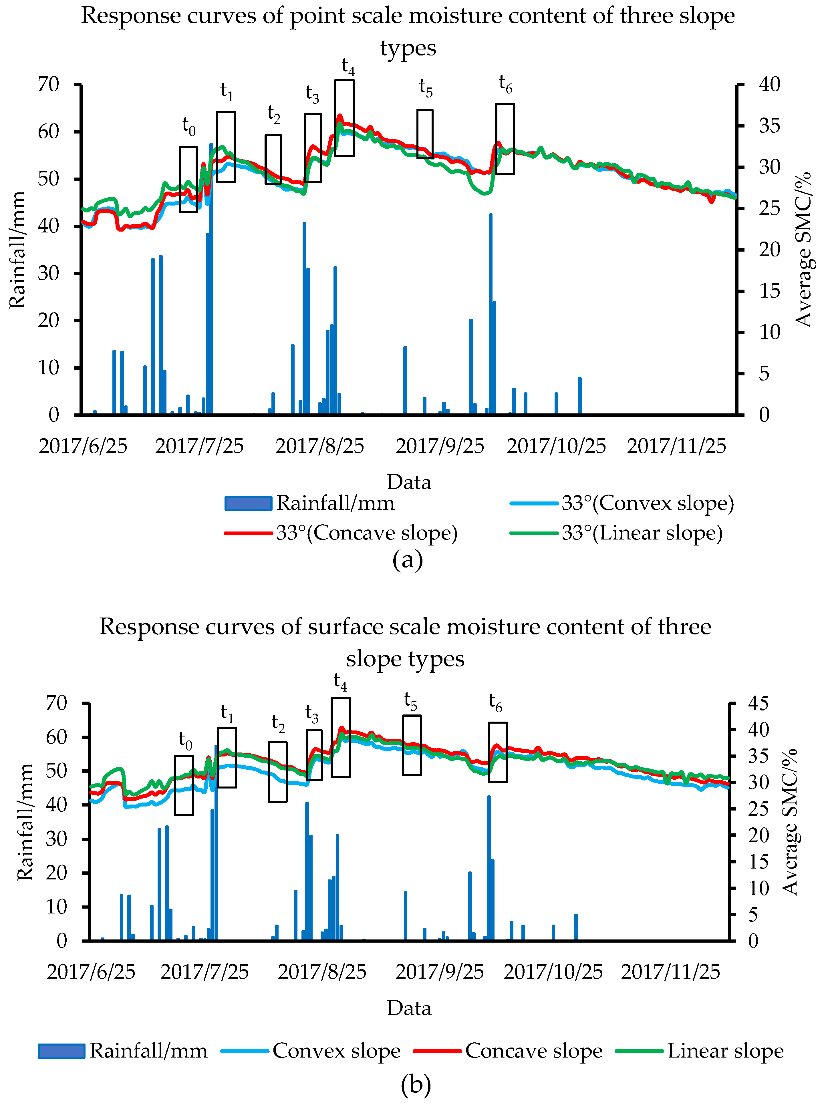
2.5. Average Soil Water Content in Two Conditions

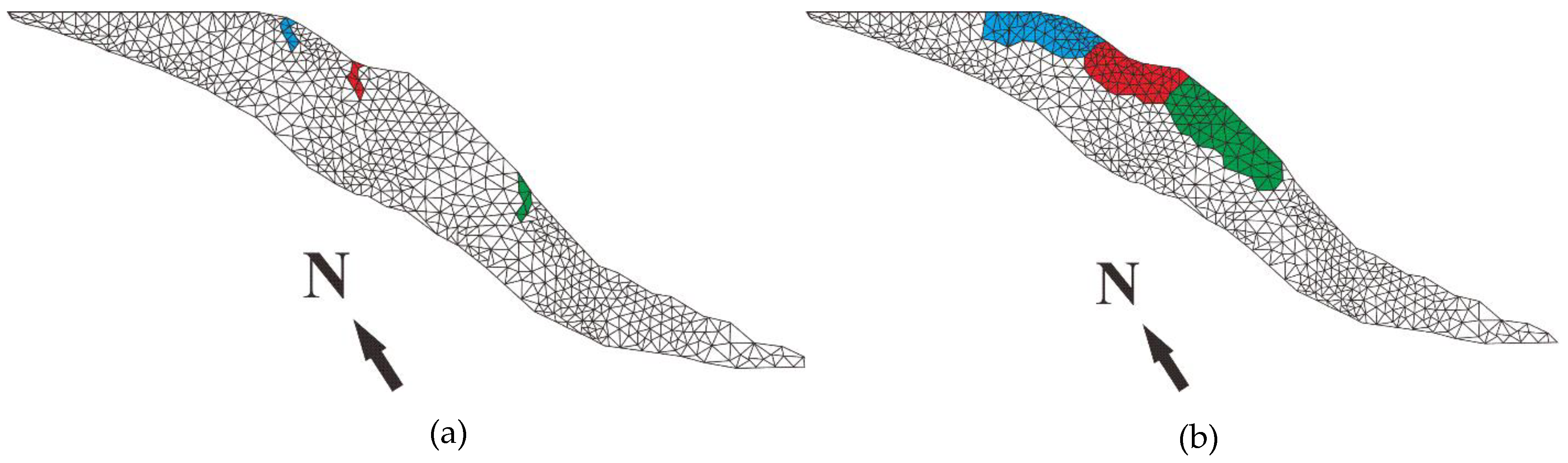
There are differences in rainfall received on the slope surface for different slope morphologies, resulting in different content and distribution of soil moisture within the slope. According to the convex morphology, concave morphology and linear morphology on the slope, it is divided into convex slope, concave slope and linear slope (Figure 5). If soil water content converted by apparent resistivity is obtained (Figure 3), it is based on rainfall characteristics under two different conditions, and the interception capacity of the three slope morphologies to surface runoff can be studied. For this purpose, the slope water content is averaged, and its expression is as follows:

$$\overline{\theta }=\frac{1}{mn}{\displaystyle \sum _{i=1}^n{\displaystyle \sum _{j=1}^m{\theta }_{ij}}}$$

(7)

$$\overline{\theta }=\frac{1}{m}{\displaystyle \sum _{j=1}^m{\theta }_j}$$

(8)

where θ_ij is the soil water content obtained at the j-th layer below the i-th electrode position for the slope; m is the number of electrodes (where m = 80); n is the data layer of apparent resistivity collection (Figure 2). The small fluctuation of soil water content in the depth is considered [34]. Where n = 8, which is a depth of 4 m, it represents the average value of soil water content obtained at each surface or point. If the soil water content field distribution of the slope is known, Equation (7) is used to obtain the average value of soil water content within 4 m underground of three slope morphologies, and Equation (8) is used to obtain the average value of soil water content within 4 m underground at a certain position of three slope morphologies. Furthermore, the interception ability of three slope morphologies to surface runoff during the rainfall process is studied by using $\overline{\theta }$ under two conditions.

3. Results and Discussion

3.1. Evaluation of the Apparent Resistivity of Slope under Different Rainfall Scenarios

Six rainfall scenarios are shown in Figure 6, and the variation of the apparent resistivity ρ in the slope during the rainfall process was analyzed. Generally, ρ was mainly distributed between 70–300 Ω m, and 1012 sets of ρ values were analyzed each time, which represents the distribution of ρ across the slope. The horizontal line was the average of ρ, and the closed circle was the median of ρ. The greater the cumulative rainfall, the average value ρ_mean, the maximum value ρ_max, the median ρ_med and the minimum value ρ_min of the overall slope apparent resistivity decreased in different degrees during rainfall. It may be that more rainwater infiltrates into the slope, resulting in the decrease of apparent resistivity within the slope. However, the smaller the cumulative rainfall, the less rainwater infiltrated into the slope, and even the loss of water was greater than the infiltrated water due to potential evaporation (Figure 4). It caused the decrease of slope water content and the increase of overall ρ during rainfall.

Specifically, when the cumulative rainfall was >70 mm, under the conditions of moderate rain, moderate rain–heavy rain and heavy rain, both ρ_med and ρ_mean decreased by about 10 Ω m. From the maximum and minimum values, ρ tended to concentrate after rainfall (Figure 6a,c,d,f). It may be that there were some fissures, such as animal and plant holes on the slope surface. When the cumulative rainfall was too large, more water infiltrated deeper into the slope along the preferential paths [35], expanding the moist area of the soil, and the wetting front moved deeper into the slope. This reduced apparent resistivity over a larger area [36], resulting in the decrease of ρ_mean and ρ_med within the entire slope. In contrast, when the cumulative rainfall was <20 mm, under the conditions of light rain and light–moderate rain, the rainfall had little effect on the distribution of ρ across the slope (Figure 6b,e). ρ_max and ρ_min remained basically unchanged and ρ_mean and ρ_med did not change significantly, and even increased. It may be that the cumulative rainfall was relatively little, and the infiltration depth was shallow. The water input owing to rainfall was less than the water loss caused by evapotranspiration, resulting in a decrease in the water content of the slope [37]. Therefore, ρ_mean and ρ_med basically remained unchanged or slightly increased after the rainfall.

In short, the apparent resistivity of the slope performed high sensitivity to the change of water content. When the cumulative rainfall was >70 mm, the evaluated apparent resistivity showed that more rainwater infiltrated into the slope, and the area with reduced apparent resistivity spread significantly. When the cumulative rainfall was <20 mm, the evaluated apparent resistivity showed that rainfall had little effect on the distribution of soil water content field within the slope, and the distribution of apparent resistivity in the region did not change much.

3.2. Two-Dimensional Time-Lapse Imaging

3.2.1. Two-Dimensional Resistivity Field

The resistivity field at the end of each rainfall was selected, corrected by temperature and presented in Figure 7. The resistivity data of the slope obtained on 24 June 2017 were used as the background field t₀ (Figure 7a). This period was in summer, the weather was dry, and the initial resistivity field distribution characteristics of the slope were clearly displayed by the imaging resistivity model [15]. In general, the resistivity near the slope toe ranged between 80–200 Ω m, and some fluctuations occurred after six rainfall events. However, the resistivity of three slope morphologies changed significantly after different rainfall events. The greater the cumulative rainfall, the more obvious the diffusion of the area where the slope resistivity decreased. It characterized the spatial and temporal variability of the apparent resistivity for the slope. From the t₀ field to the t₆ field for nearly three months, the surface temperature showed a downward trend, decreasing by about 10 °C. In the process, it also affected the potential evaporation of the slope water (Figure 4).

Specifically, the t₀ field was used as the background field. The resistivity of the slope distribution tended to be the largest, which may cause water loss due to antecedent evaporation. When the cumulative rainfall was >70 mm threshold, under the conditions of moderate rain, moderate rain–heavy rain and heavy rain, the area where the apparent resistivity decreased within the slope was relatively obvious. It may be that the potential evaporative moisture was limited, the effective precipitation was relatively abundant and more rainwater infiltrated into the slope body, resulting in its internal resistivity decreasing (Figure 7b). The area of the convex slope is particularly obvious, showing a large spatial hydrological dynamic change (Figure 7g). There may be some sinkholes, animal and plant holes distributed in this area, and it was easy for more runoff water to infiltrate into the depth of the slope along the preferential paths and spread to the surrounding area [17], thus showing a clear trend of increasing water content. Resistivity in the range of 40–100 Ω m was more diffused in the concave slope area. It is possible that the concave morphology of the slope surface was easy to converge surface runoff, resulting in preferential infiltration of water. When the cumulative rainfall was <20 mm, under the conditions of light rain and light rain–moderate rain, the slope morphology was convex, concave and linear with a limited surface resistivity reduction area. However, the resistivity distributed in the local area was small, which may be affected by the antecedent effective rainfall (Figure 4). For example, in the superficial area of a linear slope, the resistivity was distributed in the range of 200–280 Ω m (Figure 7c). It may be that the rainwater infiltrated into the soil uniformly [34] and the infiltration range was limited, which reduced the resistivity in the shallow area of the slope.

In short, excluding the partial change of resistivity caused by seasonal temperature change, the improved resistivity could better reveal the characteristics of water migration within the slope, and it performed well after temperature correction. When cumulative rainfall was <20 mm, under the conditions of light rain and light rain–moderate rain, only the area with apparent resistivity of the shallow layer of the slope decreased. When the cumulative rainfall was >70 mm, under the conditions of moderate rain, moderate rain–heavy rain and heavy rain, the areas with reduced resistivity in the shallow layers of the slope and in the three slope morphologies were more obvious [38].

3.2.2. Two-Dimensional Soil Water Content Field

The relationship between resistivity and soil water content in the study area has been described in detail by Sun [20]. In this context, the temperature compensated resistivity field can be converted into soil water content, and the relationship is as follows:

$$\rho =8.657+1021.62/\theta$$

(9)

where ρ is the resistivity of the loess pores; θ is the soil water content. Based on Equation (9), the distribution of the soil water content field could be obtained, which was plotted (Figure 8). It reflected the spatial and temporal changes of the entire slope soil water content. In general, the moisture content value was distributed in the range of 4−36%, and the slope area with moisture content concentrated in the range of 12−28% was relatively large. In addition, the ratio of the soil water content field to the background soil water content field (t_n/t₀) is shown in Figure 9 (where n = 1, …6), which was an effective method to study the changes of the soil water content field [38]. The ratio was concentrated between 0.5–2.5, indicating that compared with the background field, the moisture content increased by 2.5 times at the maximum and decreased by 50% at the minimum. This phenomenon was particularly obvious near the slope toe. It may be that after different rainfall scenarios, the rainwater was converged near the slope toe due to its own weight, which resulted in the increase of moisture content near the slope toe after different rainfall scenarios [34].

Specifically, when the cumulative rainfall was greater than 70 mm threshold, under the scenarios of moderate rain, moderate rain–heavy rain and heavy rain, the moisture content of the convex slope increased rapidly, which may be due to the distribution of more fissures and it being prone to the preferential infiltration phenomenon, resulting in a relatively obvious change in the soil water content ratio (Figure 9a,c,d,f). It reflected the rapid spread of the area with increased moisture content in the deep slope (Figure 8b,d,e,g). The area with abrupt changes in the soil water content ratio within the concave slope area was also more obvious, which may be related to the preferential infiltration of water bodies [39]. Compared with the concave slope, the linear slope had less obvious changes. It may be that the slope surface of this morphology had a weaker ability to converge surface runoff during the rainfall process than the concave slope. In addition, near the slope toe, the ratio was about 1.1–1.7 (Figure 8b and Figure 9a), indicating that more water was collected to the slope toe [15]. When the cumulative rainfall was less than 20 mm, under the scenarios of light rain and light rain–moderate rain, the areas with increased soil water content field were mainly distributed in the shallow layers of the three slope morphologies, and the distribution depth was limited (Figure 8c,f). It may be that the rainwater infiltrated uniformly into the surface of the slope, resulting in areas with a ratio greater than 1.4 in local areas (Figure 9b,e).

In summary, when the cumulative rainfall was >70 mm threshold, under the conditions of moderate rain, moderate rain–heavy rain and heavy rain, the slope was prone to preferential infiltration, which caused the water content within the slope to increase. When the cumulative rainfall was <20 mm, under the conditions of light rain and light rain–moderate rain, the slope was prone to uniform infiltration, and the infiltration depth was limited, but only in the shallow layer. It had little effect on the moisture field distribution within the slope.

3.3. Response of Water Content under Three Slopes

Based on the relationship between apparent resistivity and soil water content (Figure 3), the $\overline{\theta }$-time response curves of the 33° position points and surfaces in the three slope morphologies were presented (Figure 10). Generally, no matter what kind of rainfall process, there was hysteresis in the response of soil water content. It may take some time for water to infiltrate to the depths of the slope [9]. Therefore, under three slope morphologies, the response curves of the $\overline{\theta }$ at the point scale and the surface scale had obvious hysteresis. In addition, when the accumulated rainfall was too large, the water content curves of the three slope morphologies had obvious abrupt changes, which increased by 2–5%, respectively. When the cumulative rainfall was small, its $\overline{\theta }$ response was not obvious (Figure 10a,b).

In addition, in different rainfall processes, under the conditions of point and surface, the overall $\overline{\theta }$ responses of the three slope morphologies were: concave slope > convex slope > linear slope (Figure 10). It may be that the concave slope gradually increased the upslope angle and decreased the downslope angle [40], which made it easy to converge surface runoff, resulting in a large area for water to diffuse into the slope. Although some developed fissures were distributed on the convex slope, the slope angle gradually become larger from top to bottom, which made it easy to discharge rainwater to the outside of the slope. As a result, its overall convergence effect on surface runoff was inferior to that of the concave slope. The slope angle of the upslope and downslope of the linear slope was basically unchanged. The loess in this area was relatively uniform and the distribution of cracks was few, resulting in the weakest convergence ability of surface runoff.

3.4. Slope Failure Patterns

Slope morphology may affect the failure patterns of loess slopes [41]. Based on the six rainfall scenarios set in the rainfall simulation conditions, the water flow characteristics under three slope morphologies with different rainfall capacities were revealed. We found that no matter what kind of rainfall scenario, compared to the background field, there were different degrees of runoff distributed on the slope surface (Figure 9 and Figure 10). However, slope morphology controlled the convergence of surface runoff, which in turn affected the slope failure patterns. For example, the soil water content of the convex slope increased rapidly, and the slope toe was prone to cause stress concentration. Under rainfall conditions, the convex slope may be more prone to damage than the concave and the linear slope [42].

When the cumulative rainfall reached more than 70 mm, the preferential flow was easily excited on the concave surface of the slope, and more rainwater infiltrated into the slope, which increased the hydrodynamic pressure of the slope. This may make the internal damage area of the slope spread more obviously, resulting in local collapse at the slope toe and mid-deep landslides. At the same time, the continuous rainfall produced surface runoff on the slope, which was easy to induce local slumps. When the cumulative rainfall was less than 20 mm, the rainwater infiltrated uniformly along the slope surface and the infiltration depth was limited, resulting in less damage to the slope body. This may lead to a saturated mud flow failure pattern on the convex surface of the slope [42]. For example, Zhang and Liu [3] found that, compared with convex slopes and linear slopes, concave slopes in the loess region were more susceptible to rainwater erosion, leading to a failure pattern in the middle and deep layers of the slopes (among the 293 loess slopes investigated, there were 250 cases with a relatively large degree of damage to the slope body). In the rainfall event on 3 July 2013, Yanchuan County was taken as a case. Convex slopes (about 80% of 43 loess slopes) were more vulnerable to the influence of rainwater than concave slopes, resulting in the slope failure pattern of saturated mudflows [4].

4. Conclusions

This paper aims to present the characteristics of water flow controlled by slope morphology and its implications on slope failure patterns under different rainfall capacities, so that it provides support for the understanding of slope morphological differentiation on the overall and local failure patterns in slopes. It also can provide support for the understanding of the acquisition method of hydrological dynamics. On this basis, the Pijiagou slope was studied, and four conclusions were obtained.

The first is that the improved resistivity could better reveal the characteristics of water migration within the slope, and it performed well after temperature correction.

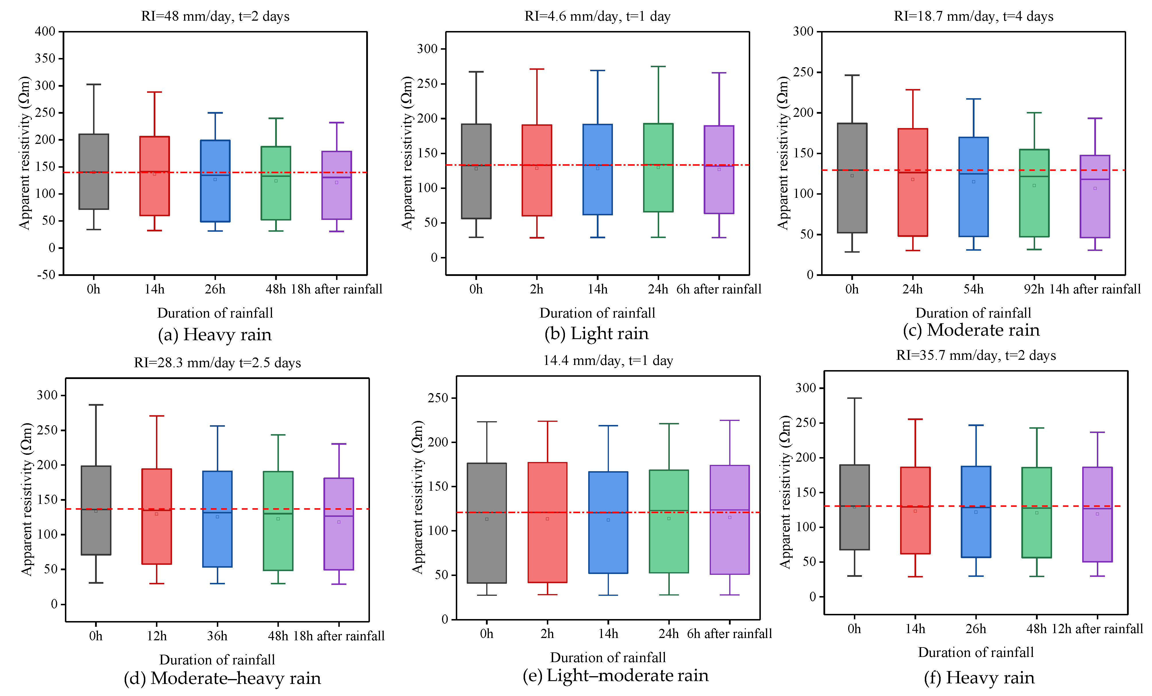
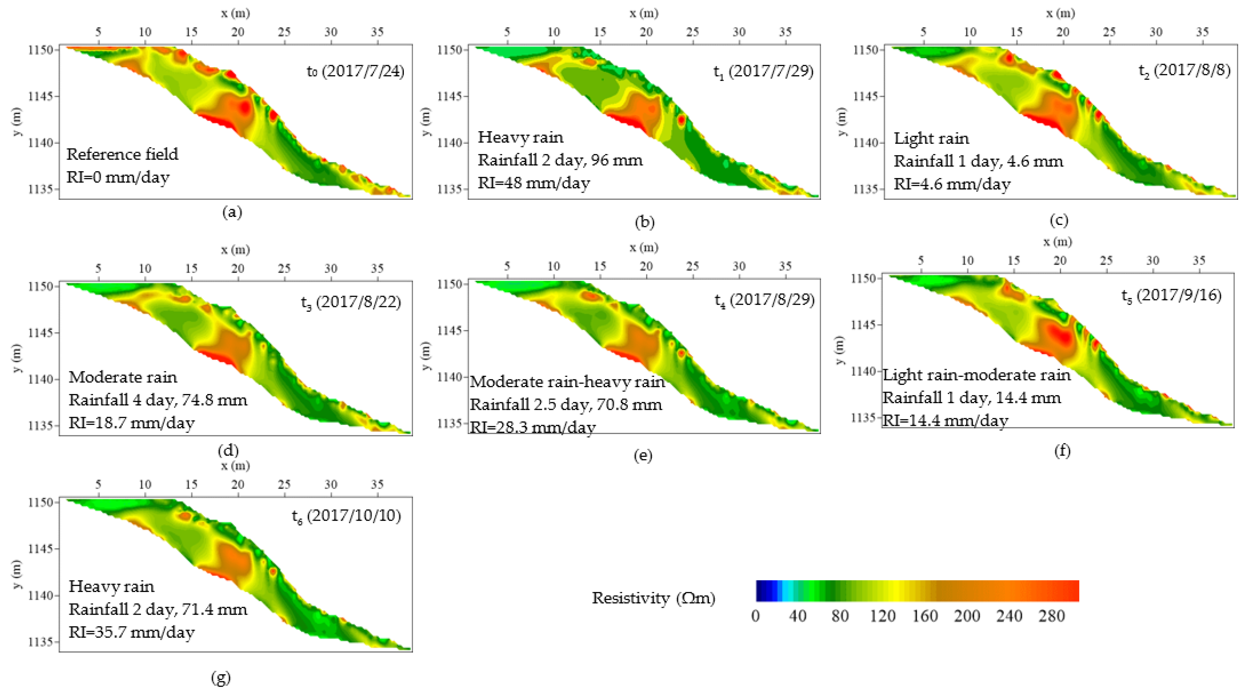
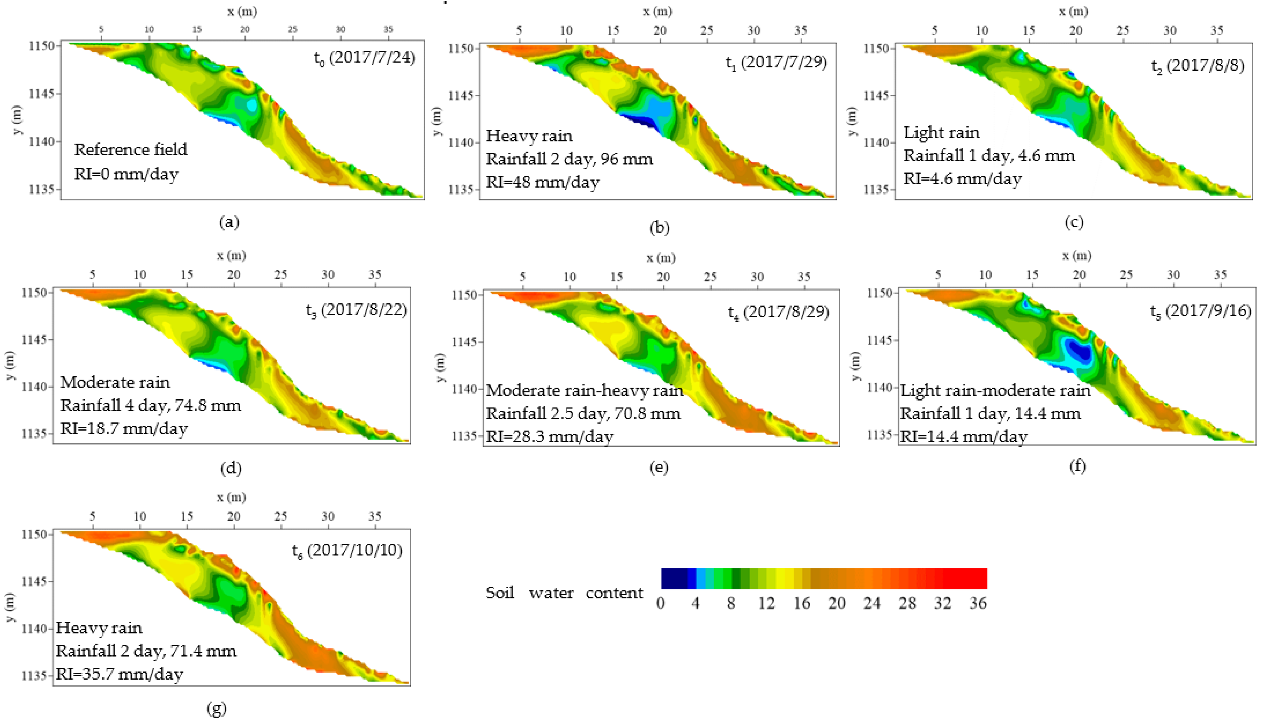
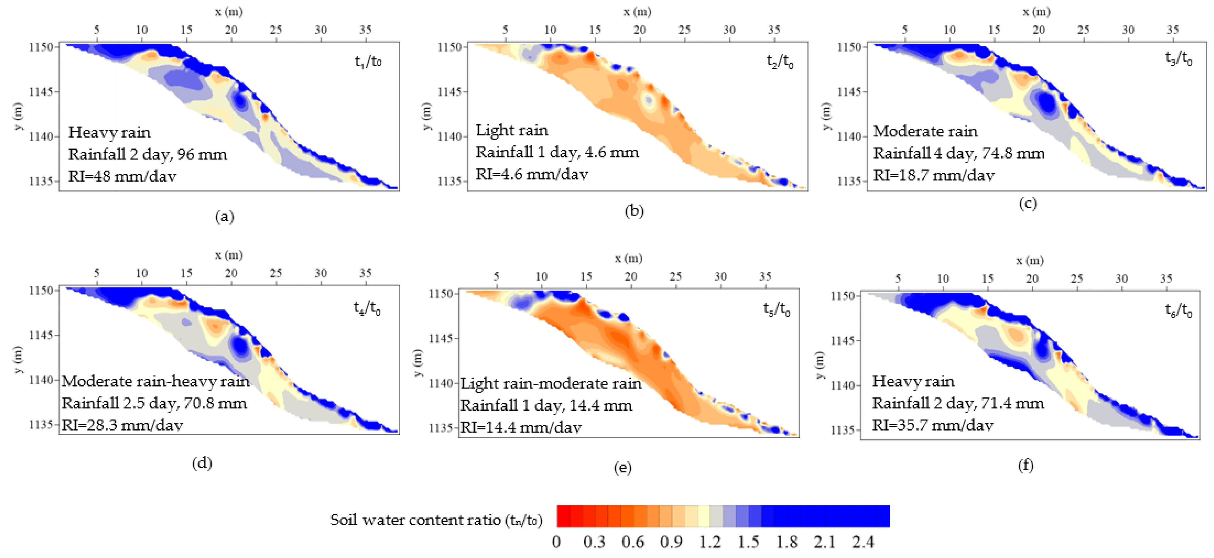
The second is that the cumulative rainfall value directly affected the characteristics of surface runoff and water infiltration. Especially when the cumulative rainfall was greater than the 70 mm threshold, under the conditions of moderate rain, moderate rain–heavy rain and heavy rain, the surface runoff quickly infiltrated along the preferential paths to the deep of the slope. However, when the cumulative rainfall value was <20 mm, it had little effect on the moisture field distribution within the slope.

The third is that if a slope was given, the interception ability of the slope morphology to the surface runoff was: concave slope > convex slope > linear slope.

The fourth is that under the conditions of light rain and light rain–moderate rain, with continuous rainfall, the convex surface of the slope is prone to be damaged by saturated mud flow. When the cumulative rainfall threshold was 70 mm, no matter if it was moderate rain, moderate rain–heavy rain or heavy rain, the preferential flow was easily excited on the concave surface of the slope, resulting in local collapse at the slope toe and the mid-deep landslides.

This outcome plays a positive role in soil and water conservation and geological disaster prevention and control considering different slope morphologies in the Chinese Loess Plateau, supporting the territorial space ecological restoration in the new era of China.

References

1. Zhou, B.B.; Wu, J.G.; Anderies, J.M. Sustainable landscapes and landscape sustainability: A tale of two concepts. Landsc. Urban Plan. 2019, 189, 274–284. [Google Scholar] [CrossRef]
2. Shu, H.P.; Ma, J.Z.; Guo, J.B.; Qi, S.; Guo, Z.Z.; Zhang, P. Effects of rainfall on surface environment and morphological characteristics in the Loess Plateau. Environ. Sci. Pollut. Res. 2020, 27, 37455–37467. [Google Scholar] [CrossRef] [PubMed]
3. Zhang, M.S.; Liu, J. Controlling factors of loess landslides in western China. Environ. Earth Sci. 2010, 59, 1671–1680. [Google Scholar] [CrossRef]
4. Wang, G.; Li, T.; Xing, X.; Zou, Y. Research on loess flow-slides induced by rainfall in July 2013 in Yan’an, NW China. Environ. Earth Sci. 2015, 73, 7933–7944. [Google Scholar] [CrossRef]
5. Feng, L.; Zhang, S.; Jin, Z.; Zhang, M.; Sun, P.; Jia, J.; Chu, G.; Hu, W. The critical mechanics of the initiation of loess flow failure and implications for landslides. Eng. Geol. 2021, 288, 106165. [Google Scholar] [CrossRef]
6. Feng, L.; Zhang, M.; Jin, Z.; Zhang, S.; Sun, P.; Gu, T.; Liu, X.; Lin, H.; An, Z.; Peng, J. The genesis, development, and evolution of original vertical joints in loess. Earth Sci. Rev. 2021, 214, 103526. [Google Scholar] [CrossRef]
7. Zhang, X.Q.; Hu, M.C.; Guo, X.Y.; Yang, H.; Zhang, Z.K.; Zhang, K.L. Effects of topographic factors on runoff and soil loss in Southwest China. CATENA 2018, 160, 394–402. [Google Scholar] [CrossRef]
8. Formetta, G.; Capparelli, G. Quantifying the three-dimensional effects of anisotropic soil horizons on hillslope hydrology and stability. J. Hydrol. 2019, 570, 329–342. [Google Scholar] [CrossRef]
9. Gu, T.F.; Zhang, M.S.; Wang, J.D.; Wang, C.-X.; Xu, Y.J.; Wang, X. The effect of irrigation on slope stability in the Heifangtai Platform, Gansu Province, China. Eng. Geol. 2019, 248, 346–356. [Google Scholar] [CrossRef]
10. Chang, Z.L.; Huang, F.M.; Huang, J.S.; Jiang, S.H.; Zhou, C.B.; Zhu, L. Experimental study of the failure mode and mechanism of loess fill slopes induced by rainfall. Eng. Geol. 2021, 280, 105941. [Google Scholar] [CrossRef]
11. Yu, L.M.; Gao, W.L.; Shamshiri, R.M.R.; Tao, S.; Ren, Y.Z.; Zhang, Y.J.; Su, G.L. Review of research progress on soil moisture sensor technology. Int. J. Agric. Biol. Eng. 2021, 14, 32–42. [Google Scholar] [CrossRef]
12. Golebiowski, T.; Piwakowski, B.; Cwiklik, M.; Bojarski, A. Application of Combined Geophysical Methods for the Examination of a Water Dam Subsoil. Water 2021, 13, 2981. [Google Scholar] [CrossRef]
13. Carrière, S.D.; Chalikakis, K. Hydrogeophysical monitoring of intense rainfall infiltration in the karst critical zone; a unique electrical resistivity tomography data set. Data Brief 2021, 40, 107762. [Google Scholar] [CrossRef] [PubMed]
14. Brunet, P.; Clément, R.; Bouvier, C. Monitoring soil water content and deficit using Electrical Resistivity Tomography (ERT)—A case study in the Cevennes area, France. J. Hydrol. 2010, 380, 146–153. [Google Scholar] [CrossRef]
15. Uhlemann, S.; Chambers, J.; Wilkinson, P.; Maurer, H.; Merritt, A.; Meldrum, P.; Kuras, O.; Gunn, D.; Smith, A.; Dijkstra, T. Four-dimensional imaging of moisture dynamics during landslide reactivation. J. Geophys. Res. Earth Surf. 2017, 122, 398–418. [Google Scholar] [CrossRef] [Green Version]
16. Zhao, K.Y.; Xu, Q.; Liu, F.Z.; Xiu, D.; Ren, X. Field monitoring of preferential infiltration in loess using time-lapse electrical resistivity tomography. J. Hydrol. 2020, 591, 125278. [Google Scholar] [CrossRef]
17. Beven, K.; Germann, P. Macropores and water flow in soils revisited. Water Resour. Res. 2013, 49, 3071–3092. [Google Scholar] [CrossRef] [Green Version]
18. Lehmann, P.; Gambazzi, F.; Suski, B.; Baron, L.; Askarinejad, A.; Springman, S.M.; Holliger, K.; Or, D. Evolution of soil wetting patterns preceding a hydrologically induced landslide inferred from electrical resistivity survey and point measurements of volumetric water content and pore water pressure. Water Resour. Res. 2013, 49, 7992–8004. [Google Scholar] [CrossRef]
19. Ramos Filho, G.M.; Coelho, V.H.R.; da Silva Freitas, E.; Xuan, Y.; das Neves Almeida, C. An improved rainfall-threshold approach for robust prediction and warning of flood and flash flood hazards. Nat. Hazards 2021, 105, 2409–2429. [Google Scholar] [CrossRef]
20. Sun, P.; Zhang, M.S.; Gu, T.F. In-situ monitoring of water infiltration for loess slopes based on improved electrical resistivity tomography technique. J. Lanzhou Univ. 2020, 56, 211–218. (In Chinese) [Google Scholar]
21. Cimpoiasu, M.O.; Kuras, O.; Wilkinson, P.B.; Pridmore, T.; Mooney, S.J. Hydrodynamic characterization of soil compaction using integrated electrical resistivity and X-ray computed tomography. Vadose Zone J. 2021, 20, vzj2.20109. [Google Scholar] [CrossRef]
22. Loke, M.H.; Barker, R.D. Rapid least-squares inversion of apparent resistivity pseudosections by a quasi-Newton method1. Geophys. Prospect. 1996, 44, 131–152. [Google Scholar] [CrossRef]
23. Jodry, C.; Lopes, S.P.; Fargier, Y.; Sanchez, M.; Cote, P. 2D-ERT monitoring of soil moisture seasonal behaviour in a river levee: A case study. J. Appl. Geophys. 2019, 167, 140–151. [Google Scholar] [CrossRef] [Green Version]
24. de Groot-Hedlin, C.; Constable, S. Occam’s inversion to generate smooth, two-dimensional models from magnetotelluric data. Geophysics 1990, 55, 1613–1624. [Google Scholar] [CrossRef]
25. Gupta, P.K.; Niwas, S.; Gaur, V.K. Straightforward inversion of vertical electrical sounding data. Geophysics 1997, 62, 775–785. [Google Scholar] [CrossRef] [Green Version]
26. Archie, G.E. The electrical resistivity log as an aid in determining some reservoir characteristics. Trans. AIME 1942, 146, 54–62. [Google Scholar] [CrossRef]
27. Yamakawa, Y.; Kosugi, K.I.; Katsura, S.Y.; Masaoka, N.; Mizuyama, T. Spatial and temporal monitoring of water content in weathered granitic bedrock using electrical resistivity imaging. Vadose Zone J. 2012, 11, vzj2011.0029. [Google Scholar] [CrossRef]
28. Hayley, K.; Bentley, L.R.; Gharibi, M.; Nightingale, M. Low temperature dependence of electrical resistivity: Implications for near surface geophysical monitoring. Geophys. Res. Lett. 2007, 34. [Google Scholar] [CrossRef]
29. Ma, R.; McBratney, A.; Whelan, B.; Minasny, B.; Short, M. Comparing temperature correction models for soil electrical conductivity measurement. Precis. Agric. 2011, 12, 55–66. [Google Scholar] [CrossRef]
30. Hayashi, M. Temperature-electrical conductivity relation of water for environmental monitoring and geophysical data inversion. Environ. Monit. Assess. 2004, 96, 119–128. [Google Scholar] [CrossRef]
31. Keller, G.V.; Frischknecht, F.C. Electrical Methods in Geophysical Prospecting; Pergamon Press: Oxford, UK, 1966; 517p. [Google Scholar]
32. Blaney, H.F.; Criddle, W.D. Determining Consumptive Use and Irrigation Water Requirements; US Department of Agriculture: Washington, DC, USA, 1962.
33. Ponce, V.M. Engineering Hydrology: Principles and Practices; Prentice Hall Englewood Cliffs, NJ: New York, NY, USA, 1989; Volume 640. [Google Scholar]
34. Hou, X.; Vanapalli, S.K.; Li, T. Water infiltration characteristics in loess associated with irrigation activities and its influence on the slope stability in Heifangtai loess highland, China. Eng. Geol. 2018, 234, 27–37. [Google Scholar] [CrossRef]
35. Nimmo, J.R. The processes of preferential flow in the unsaturated zone. Soil Sci. Soc. Am. J. 2021, 85, 1–27. [Google Scholar] [CrossRef]
36. Zeng, R.; Meng, X.; Zhang, F.; Wang, S.; Cui, Z.; Zhang, M.; Zhang, Y.; Chen, G. Characterizing hydrological processes on loess slopes using electrical resistivity tomography–A case study of the Heifangtai Terrace, Northwest China. J. Hydrol. 2016, 541, 742–753. [Google Scholar] [CrossRef]
37. Merritt, A.J.; Chambers, J.E.; Murphy, W.; Wilkinson, P.B.; West, L.J.; Uhlemann, S.; Meldrum, P.I.; Gunn, D. Landslide activation behaviour illuminated by electrical resistance monitoring. Earth Surf. Processes Landf. 2018, 43, 1321–1334. [Google Scholar] [CrossRef]
38. Chambers, J.; Gunn, D.; Wilkinson, P.; Meldrum, P.; Haslam, E.; Holyoake, S.; Kirkham, M.; Kuras, O.; Merritt, A.; Wragg, J. 4D electrical resistivity tomography monitoring of soil moisture dynamics in an operational railway embankment. Near Surf. Geophys. 2014, 12, 61–72. [Google Scholar] [CrossRef] [Green Version]
39. Kukemilks, K.; Wagner, J.-F.; Saks, T.; Brunner, P. Conceptualization of preferential flow for hillslope stability assessment. Hydrogeol. J. 2018, 26, 439–450. [Google Scholar] [CrossRef]
40. Wood, A. The development of hillside slopes. Proc. Geol. Assoc. 1942, 53, 128–140. [Google Scholar] [CrossRef]
41. Reid, M.E.; Iverson, R.M. Gravity-driven groundwater flow and slope failure potential: 2. Effects of slope morphology, material properties, and hydraulic heterogeneity. Water Resour. Res. 1992, 28, 939–950. [Google Scholar] [CrossRef]
42. Sun, C.W.; Chai, J.R.; Xu, Z.G.; Qin, Y. 3D Stability Charts for Convex and Concave Slopes in Plan View with Homogeneous Soil Based on the Strength-Reduction Method. Int. J. Geomech. 2017, 17, 06016034. [Google Scholar] [CrossRef]
Figure 1. Study site: (a) a map of the Chinese Loess Plateau, showing the locations of the Baota District; (b) site plan showing aerial photographs of the study area and the location of the 2D electrical resistivity tomography imaging array, other monitoring facilities and borehole locations; (c) electrical resistivity tomography layout plan of the slope in the study area. ERT is the acronym of electrical resistivity tomography.
Water 14 01271 g001
Figure 2. Schematic diagram of apparent resistivity acquisition.
Water 14 01271 g002
Figure 3. Soil water content–apparent resistivity relationship for the formation determined from in situ monitoring and fitted by Archie model.
Water 14 01271 g003
Figure 4. Weekly precipitation, weekly effective precipitation and weekly average temperature measured. The arrows indicate the measurement moments for the six groups of apparent resistivity.
Water 14 01271 g004
Figure 5. The division area of the slope morphology under two conditions: (a) point scale (33°); (b) surface scale.
Water 14 01271 g005
Figure 6. Spatial variability of apparent resistivity of the slope under different rainfall scenarios. The red dashed lines represent mean apparent resistivity for all points (n = 2769) before the rainfall. The red dotted lines indicate the average measured value for the apparent resistivity of the slope background.
Water 14 01271 g006
Figure 7. Temperature corrected 2D apparent resistivity model sections (x = Distance, y = Elevation). (ag) is the distribution of slope apparent resistivity field under different rainfall conditions.
Water 14 01271 g007
Figure 8. Soil water content field based on the conversion of resistivity (x = Distance, y = Elevation). (ag) is the distribution of slope soil water content field under different rainfall conditions.
Water 14 01271 g008
Figure 9. Soil water content ratio field plots calculated using the relationship between resistivity and soil water content (x = Distance, y = Elevation). (af) is the distribution of slope soil water content ratio field under different rainfall conditions.
Water 14 01271 g009
Figure 10. The time sequence diagrams of changing with time under two conditions were as follows: (a) concave slope, convex slope and linear slope at 33° position (within 4 m from the ground); (b) concave slope, convex slope and linear slope (within 4 m from the ground).
Water 14 01271 g010