
Pipeline Leakage Detection and Localization Using a Reliable Pipeline-Mechanism Model Incorporating a Bayesian Model Updating Approach


Abstract
:1. Introduction
2. Methods
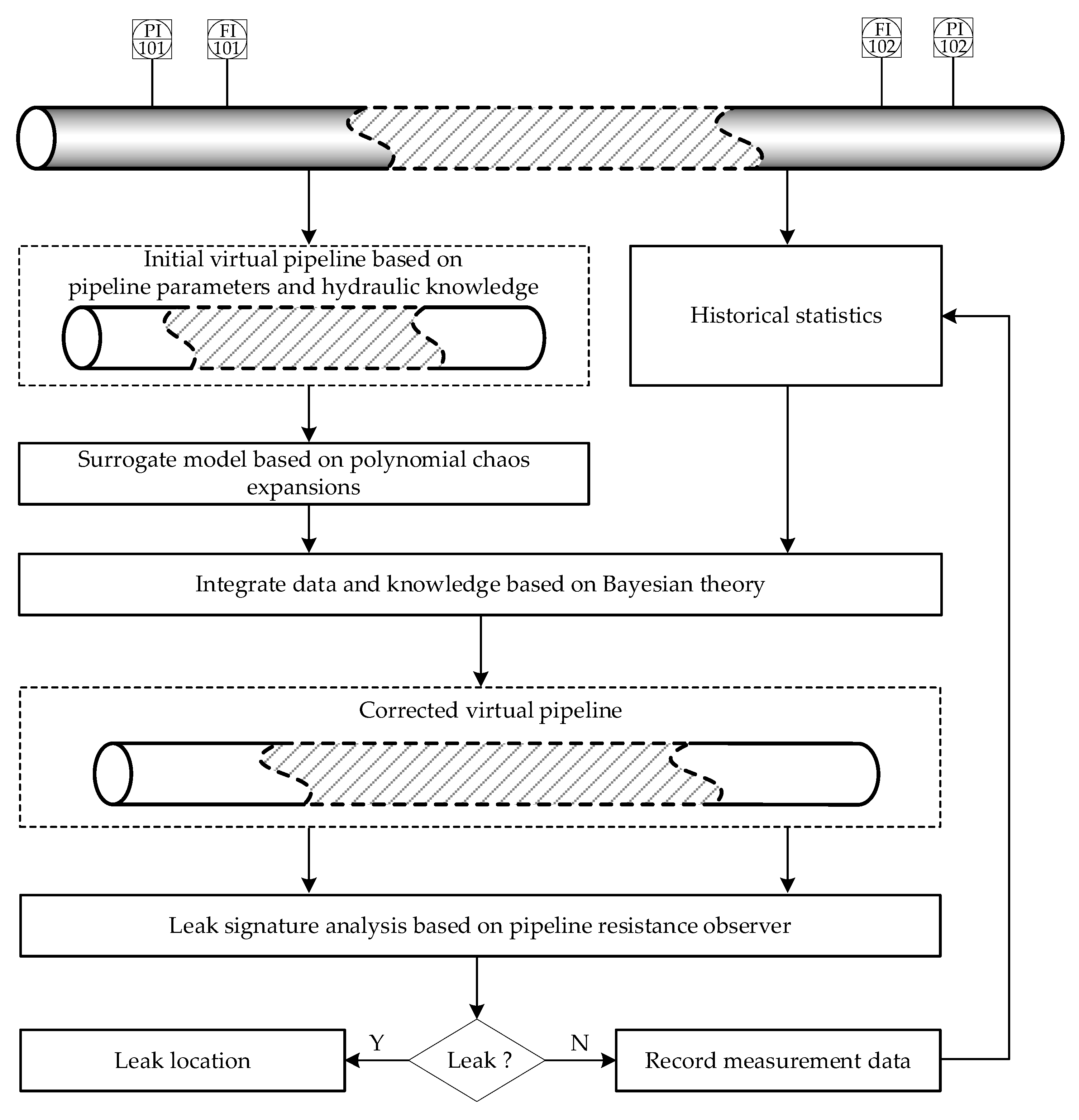
2.1. Pipeline-Mechanism Model
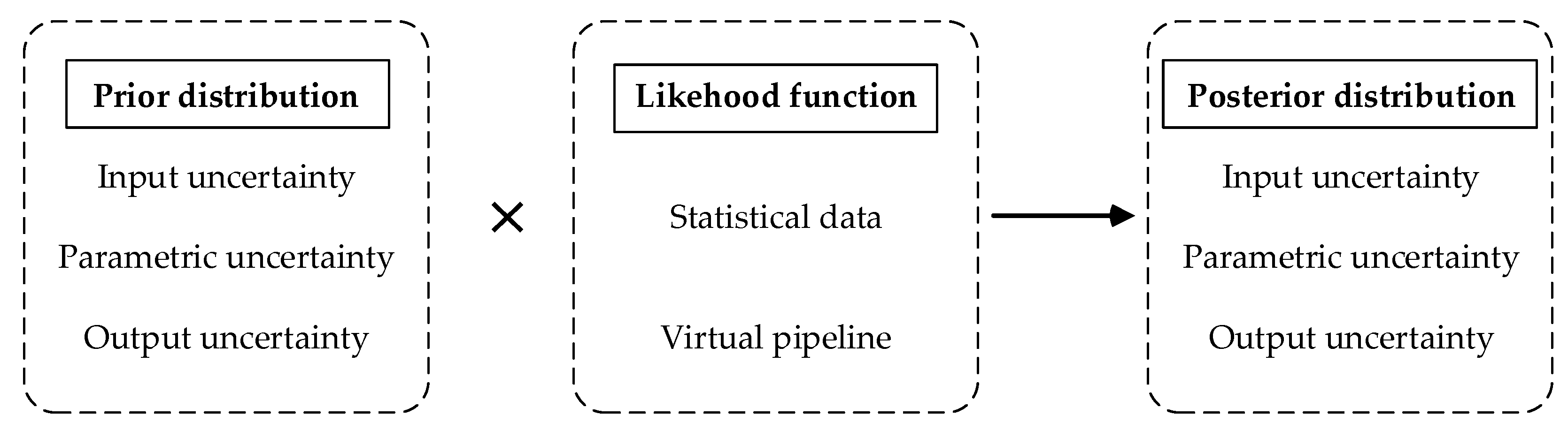
2.2. Bayesian Fusion Method
2.2.1. Bayesian Method
2.2.2. Prior Distribution
2.2.3. Likelihood Function
2.2.4. Posterior Distribution
2.3. Surrogate Model
2.4. Sampling Method
2.5. Leak Detection
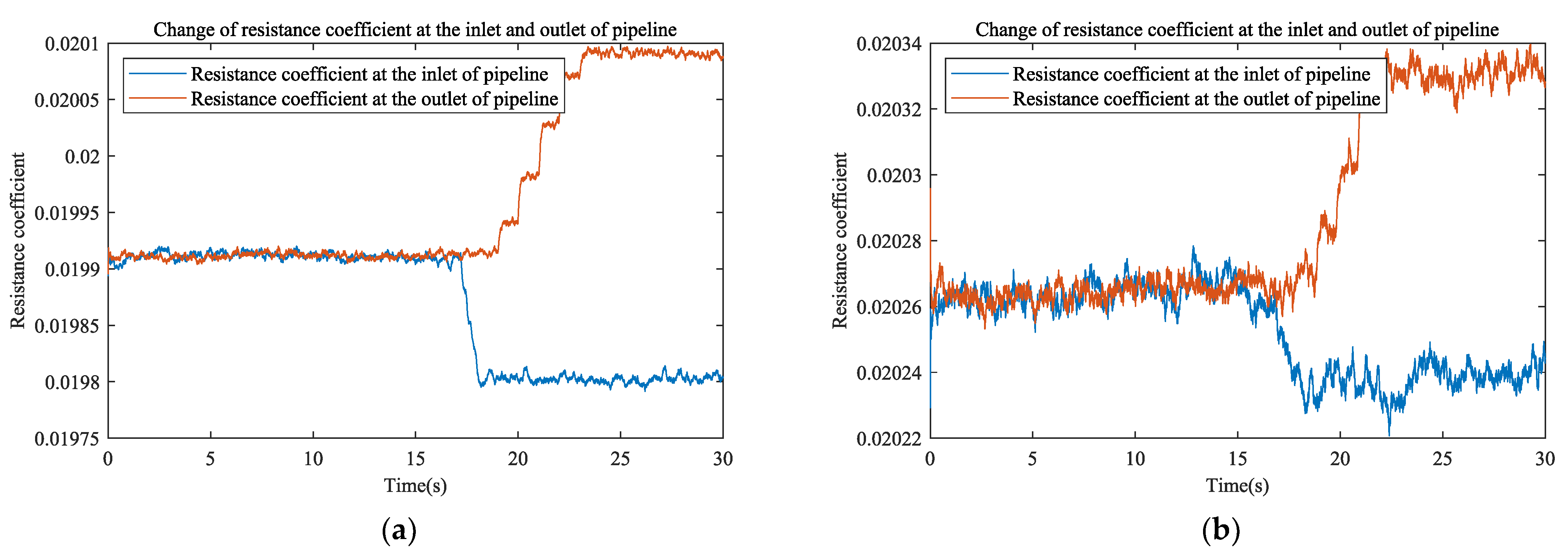
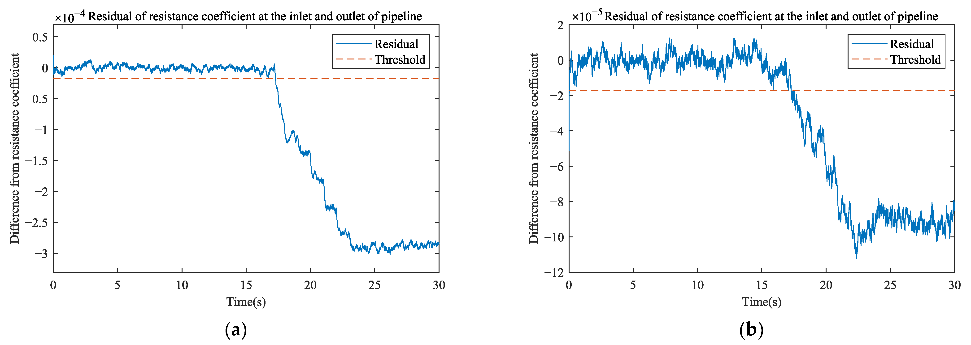
2.5.1. Pipeline Resistance Coefficient Observer
2.5.2. Leak Detection
2.6. Leak Location
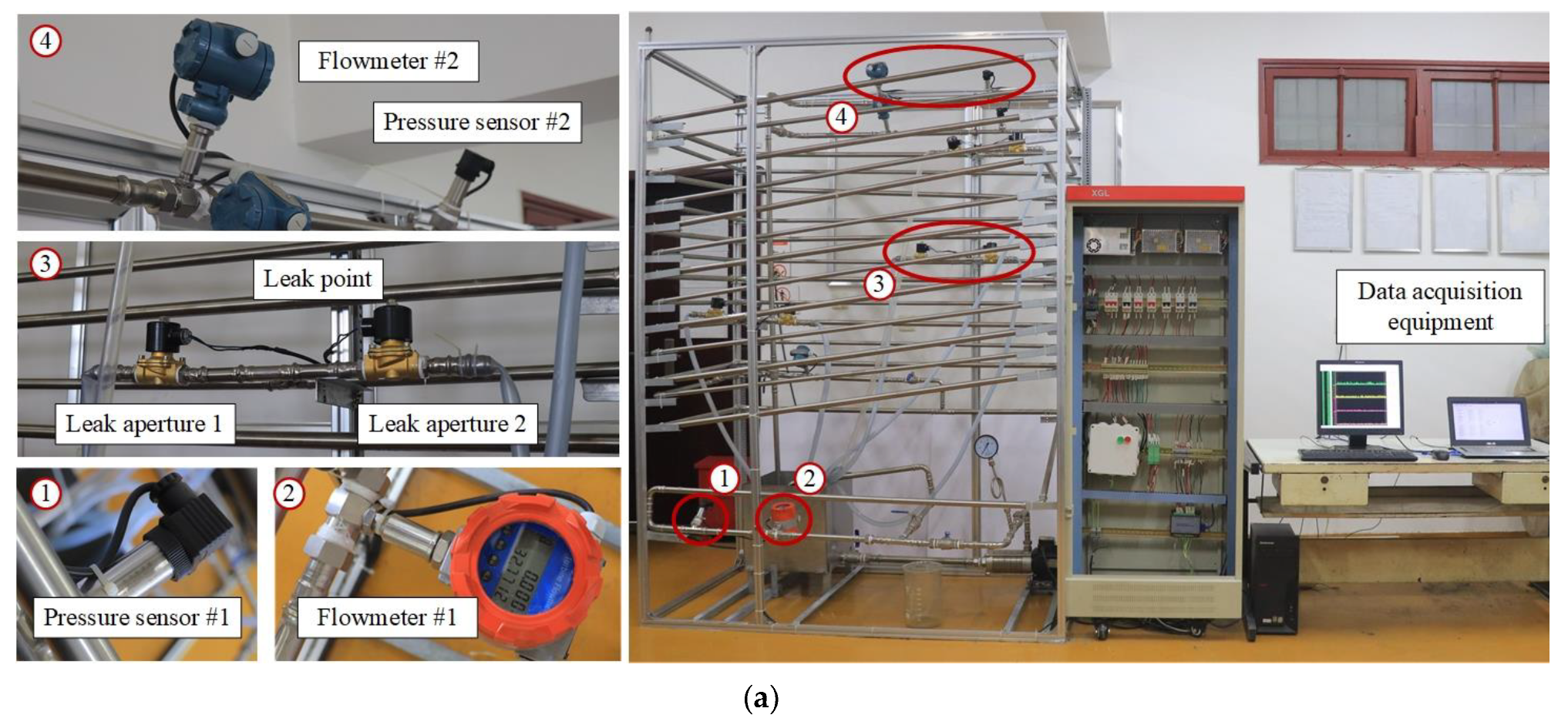
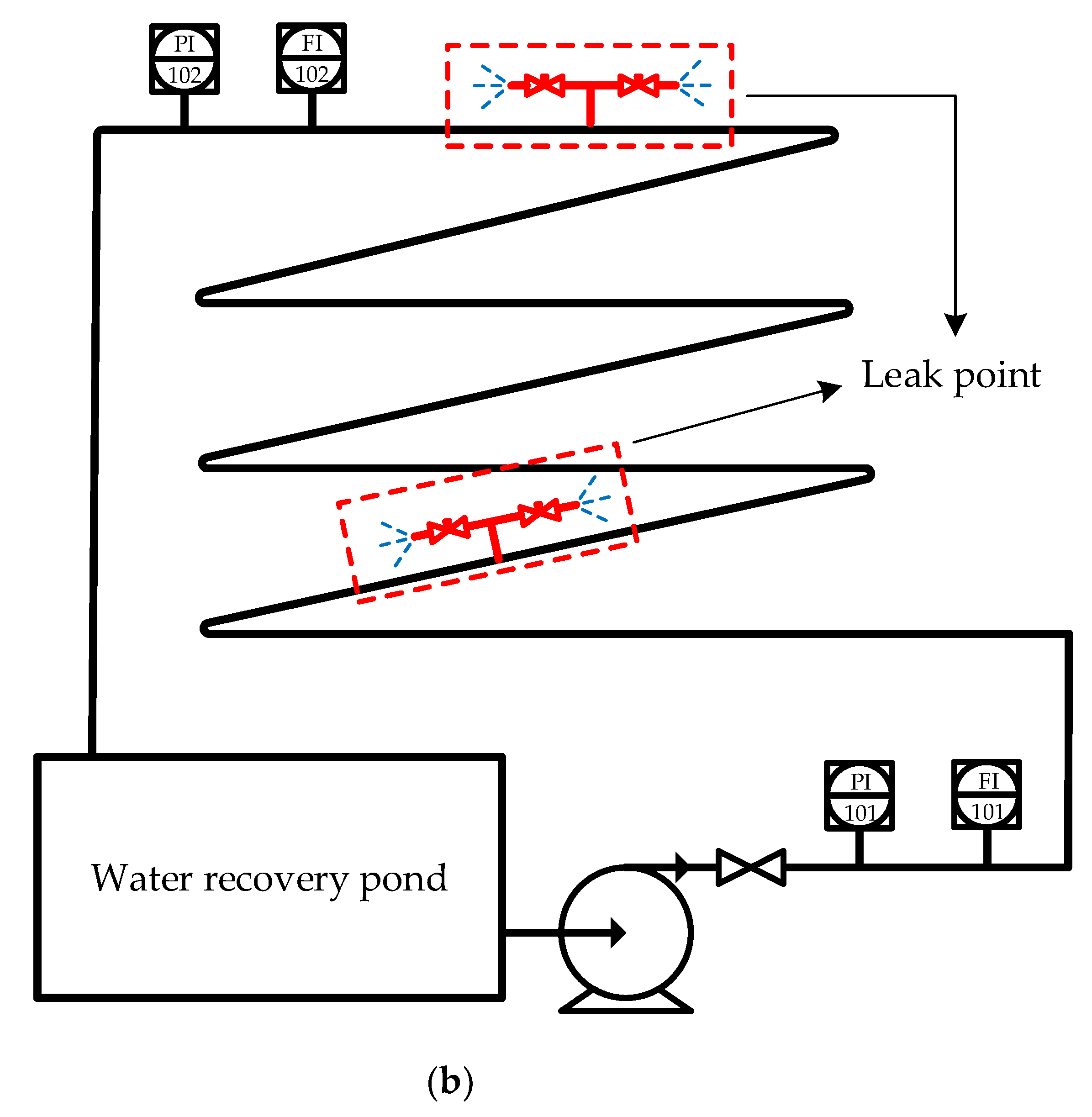
3. Experiments and Results
3.1. Experimental Device
3.2. Model Validation
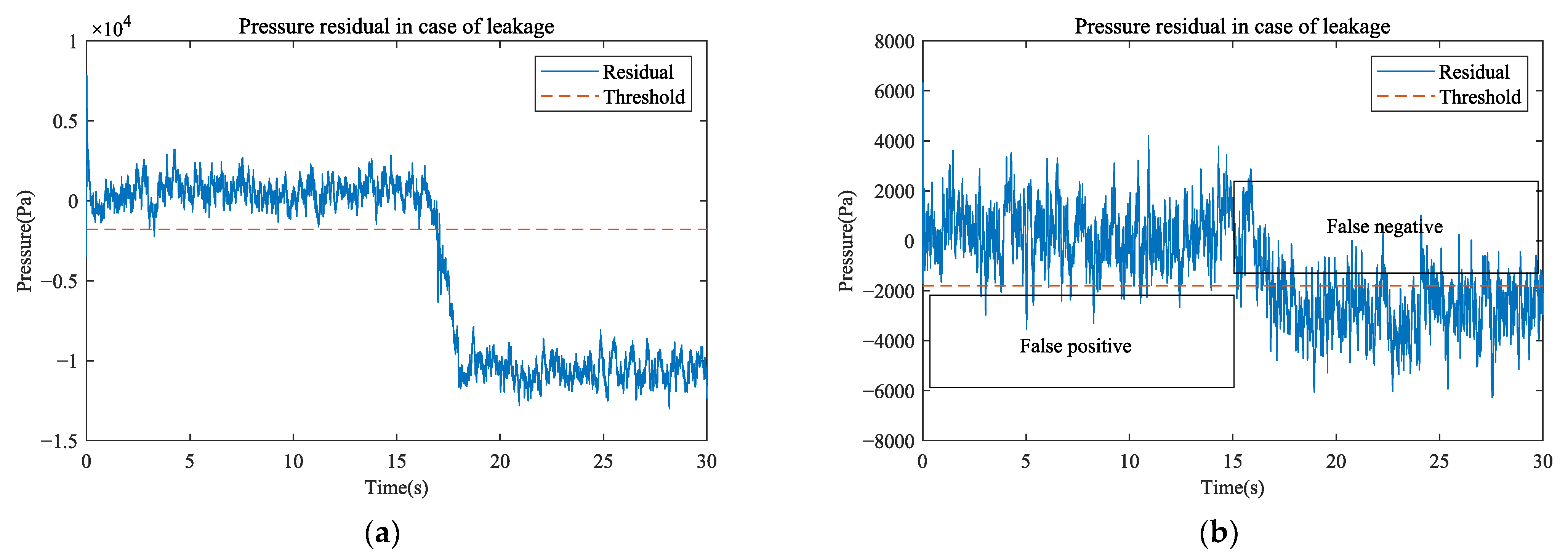
3.3. Leak Detection
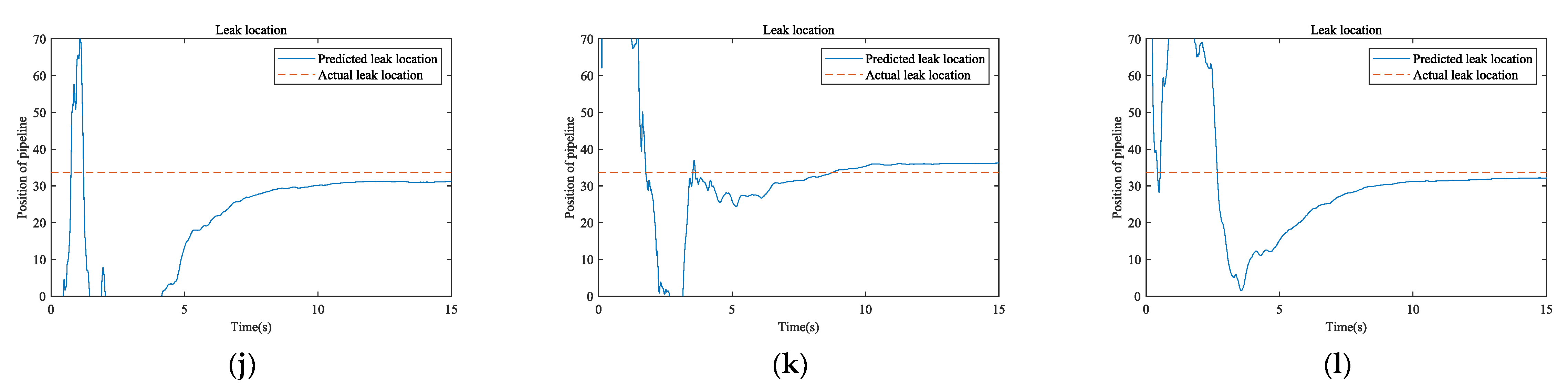
3.4. Leak Location
4. Discussion and Conclusions
Author Contributions
Funding
Institutional Review Board Statement
Informed Consent Statement
Data Availability Statement
Conflicts of Interest
References
- Moubayed, A.; Sharif, M.; Luccini, M.; Primak, S.; Shami, A. Water Leak Detection Survey: Challenges & Research Opportunities Using Data Fusion & Federated Learning. IEEE Access 2021, 9, 40595–40611. [Google Scholar]
- Preetha, P.; Eldhose, N.V. Survey on Recent Trends in Pipeline Monitoring to Detect and Localize Leaks using Sensors. Int. J. Adv. Sci. Technol. 2020, 29, 3199–3210. [Google Scholar]
- Lu, H.; Iseley, T.; Behbahani, S.; Fu, L. Leakage detection techniques for oil and gas pipelines: State-of-the-art. Tunn. Undergr. Space Technol. 2020, 98, 103249. [Google Scholar] [CrossRef]
- Hyun, S.Y.; Jo, Y.S.; Oh, H.C.; Kim, S.Y.; Kim, Y.S. The laboratory scaled-down model of a ground-penetrating radar for leak detection of water pipes. Meas. Sci. Technol. 2007, 18, 2791. [Google Scholar] [CrossRef]
- Xu, C.; Du, S.; Gong, P.; Li, Z.; Song, G. An Improved Method for Pipeline Leakage Localization with a Single Sensor Based on Modal Acoustic Emission and Empirical Mode Decomposition with Hilbert Transform. IEEE Sens. J. 2020, 20, 5480–5491. [Google Scholar] [CrossRef]
- Ibrahim, K.; Tariq, S.; Bakhtawar, B.; Zayed, T. Application of fiber optics in water distribution networks for leak detection and localization: A mixed methodology-based review. H2Open J. 2021, 4, 244–261. [Google Scholar] [CrossRef]
- Zhiwang, Z.; Qiang, W.; Xiaohong, G.U.; Ya, Z.; Kai, Z. Analysis on underground water pipes multi-point leakage location method based on distributed optical fiber. J. Appl. Opt. 2020, 41, 228–234. [Google Scholar] [CrossRef]
- Wu, D.; Liu, Z.; Wang, X.; Su, L. Composite magnetic flux leakage detection method for pipelines using alternating magnetic field excitation. NDT E Int. 2017, 91, 148–155. [Google Scholar] [CrossRef]
- Ge, C.; Wang, G.; Hao, Y. Analysis of the smallest detectable leakage flow rate of negative pressure wave-based leak detection systems for liquid pipelines. Comput. Chem. Eng. 2008, 32, 1669–1680. [Google Scholar] [CrossRef]
- Li, J.; Zheng, Q.; Qian, Z.; Yang, X. A novel location algorithm for pipeline leakage based on the attenuation of negative pressure wave. Process Saf. Environ. Protect. 2019, 123, 309–316. [Google Scholar] [CrossRef]
- Abdulshaheed, A.; Mustapha, F.; Ghavamian, A. A pressure-based method for monitoring leaks in a pipe distribution system: A Review. Renew. Sustain. Energy Rev. 2017, 69, 902–911. [Google Scholar] [CrossRef]
- Liou, J.C. Leak detection by mass balance effective for Norman wells line. Oil Gas J. 1996, 94, 220623. [Google Scholar]
- Xu, X.; Karney, B. An Overview of Transient Fault Detection Techniques. In Modeling and Monitoring of Pipelines and Networks: Advanced Tools for Automatic Monitoring and Supervision of Pipelines; Verde, C., Torres, L., Eds.; Springer: Berlin/Heidelberg, Germany, 2017; pp. 13–37. [Google Scholar]
- Duan, H.F.; Pan, B.; Wang, M.; Chen, L.; Zheng, F.; Zhang, Y. State-of-the-art review on the transient flow modeling and utilization for urban water supply system (UWSS) management. J. Water Supply Res. Technol.-Aqua 2020, 69, 858–893. [Google Scholar] [CrossRef]
- Chen, Q.; Xing, X.; Jin, C.; Zuo, L.; Wu, J.; Wang, W. A novel method for transient leakage flow rate calculation of gas transmission pipelines. J. Nat. Gas Sci. Eng. 2020, 77, 103261. [Google Scholar] [CrossRef]
- Liu, E.; Kuang, J.; Peng, S.; Liu, Y. Transient operation optimization technology of gas transmission pipeline: A case study of west-east gas transmission pipeline. IEEE Access 2019, 7, 112131–112141. [Google Scholar] [CrossRef]
- Soares, A.K.; Covas, D.I.; Reis, L.F.R. Leak detection by inverse transient analysis in an experimental PVC pipe system. J. Hydroinform. 2011, 13, 153–166. [Google Scholar] [CrossRef]
- Rubio Scola, I.; Besançon, G.; Georges, D. Blockage and leak detection and location in pipelines using frequency response optimization. J. Hydraul. Eng. 2017, 143, 04016074. [Google Scholar] [CrossRef]
- Covas, D.; Ramos, H.; De Almeida, A.B. Standing wave difference method for leak detection in pipeline systems. J. Hydraul. Eng. 2005, 131, 1106–1116. [Google Scholar] [CrossRef]
- Sun, J.; Wang, R.; Duan, H.-F. Multiple-fault detection in water pipelines using transient-based time-frequency analysis. J. Hydroinform. 2016, 18, 975–989. [Google Scholar] [CrossRef] [Green Version]
- Zeng, W.; Gong, J.; Cook, P.R.; Arkwright, J.W.; Simpson, A.R.; Cazzolato, B.S.; Zecchin, A.C.; Lambert, M.F. Leak detection for pipelines using in-pipe optical fiber pressure sensors and a paired-IRF technique. J. Hydraul. Eng. 2020, 146, 06020013. [Google Scholar] [CrossRef]
- Duan, H.F. Transient frequency response based leak detection in water supply pipeline systems with branched and looped junctions. J. Hydroinform. 2016, 19, 17–30. [Google Scholar] [CrossRef]
- Meniconi, S.; Capponi, C.; Frisinghelli, M.; Brunone, B. Leak detection in a real transmission main through transient tests: Deeds and misdeeds. Water Resour. Res. 2021, 57, e2020WR027838. [Google Scholar] [CrossRef]
- Brunone, B.; Capponi, C.; Meniconi, S. Design criteria and performance analysis of a smart portable device for leak detection in water transmission mains. Measurement 2021, 183, 109844. [Google Scholar] [CrossRef]
- Wang, Z.; He, X.; Shen, H.; Fan, S.; Zeng, Y. Multi-source information fusion to identify water supply pipe leakage based on SVM and VMD. Inf. Process. Manag. 2022, 59, 102819. [Google Scholar] [CrossRef]
- Zadkarami, M.; Shahbazian, M.; Salahshoor, K. Pipeline leakage detection and isolation: An integrated approach of statistical and wavelet feature extraction with multi-layer perceptron neural network (MLPNN). J. Loss Prev. Process Ind. 2016, 43, 479–487. [Google Scholar] [CrossRef]
- Cruz, R.P.D.; Silva, F.V.d.; Fileti, A.M.F. Machine learning and acoustic method applied to leak detection and location in low-pressure gas pipelines. Clean Technol. Environ. Policy 2020, 22, 627–638. [Google Scholar] [CrossRef]
- Pietrucha-Urbanik, K.; Studziński, A. Qualitative analysis of the failure risk of water pipes in terms of water supply safety. Eng. Fail. Anal. 2019, 95, 371–378. [Google Scholar] [CrossRef]
- Geiger, G.; Werner, T.; Matko, D. Knowledge-Based Leak Monitoring for Pipelines. IFAC Proc. Vol. 2001, 34, 249–254. [Google Scholar] [CrossRef]
- Soldevila, A.; Blesa, J.; Tornil-Sin, S.; Duviella, E.; Fernandez-Canti, R.M.; Puig, V. Leak localization in water distribution networks using a mixed model-based/data-driven approach. Control Eng. Pract. 2016, 55, 162–173. [Google Scholar] [CrossRef] [Green Version]
- Wang, J.; Wang, T.; Wang, J. Hybrid modelling for leak detection of long-distance gas transport pipeline. Insight-Non-Destr. Test. Cond. Monit. 2013, 55, 372–381. [Google Scholar]
- Collins, J.D.; Thomson, W.T. The eigenvalue problem for structural systems with statistical properties. AIAA J. 1969, 7, 642–648. [Google Scholar] [CrossRef]
- Hart, G.C.; Collins, J.D. The treatment of randomness in finite element modeling. SAE Trans. 1970, 79, 2509–2520. [Google Scholar]
- Beck, J.L.; Au, S.-K. Bayesian updating of structural models and reliability using Markov chain Monte Carlo simulation. J. Eng. Mech. 2002, 128, 380–391. [Google Scholar] [CrossRef]
- Kennedy, M.C.; O’Hagan, A. Bayesian calibration of computer models. J. R. Stat. Soc. Ser. B—Stat. Methodol. 2001, 63, 425–464. [Google Scholar] [CrossRef]
- Auranen, T.; Nummenmaa, A.; Hamalainen, M.S.; Jaaskelainen, I.P.; Lampinen, J.; Vehtari, A.; Sams, M. Bayesian analysis of the neuromagnetic inverse problem with ℓp-norm priors. Neuroimage 2005, 26, 870–884. [Google Scholar] [CrossRef] [PubMed]
- Keats, A.; Yee, E.; Lien, F.S. Bayesian inference for source determination with applications to a complex urban environment. Atmos. Environ. 2007, 41, 465–479. [Google Scholar] [CrossRef]
- Dowd, M.; Meyer, R. A Bayesian approach to the ecosystem inverse problem. Ecol. Model. 2003, 168, 39–55. [Google Scholar] [CrossRef] [Green Version]
- Fleming, K.N. Markov models for evaluating risk-informed in-service inspection strategies for nuclear power plant piping systems. Reliab. Eng. Syst. Saf. 2004, 83, 27–45. [Google Scholar] [CrossRef]
- Rougier, J. Probabilistic leak detection in pipelines using the mass imbalance approach. J. Hydraul. Res. 2005, 43, 556–566. [Google Scholar] [CrossRef]
- Vrugt, J.A.; ter Braak, C.J.F.; Diks, C.G.H.; Robinson, B.A.; Hyman, J.M.; Higdon, D. Accelerating Markov Chain Monte Carlo Simulation by Differential Evolution with Self-Adaptive Randomized Subspace Sampling. Int. J. Nonlinear Sci. Numer. Simul. 2009, 10, 273–290. [Google Scholar] [CrossRef]
- Laloy, E.; Vrugt, J. High-dimensional posterior exploration of hydrologic models using multiple-try DREAM(ZS) and high-performance computing. Water Resour. Res. 2012, 48, W01526. [Google Scholar] [CrossRef] [Green Version]
- Chaudhry, M.H. Applied Hydraulic Transients; Springer: Berlin/Heidelberg, Germany, 1979. [Google Scholar]
- Wylie, E.B.; Streeter, V.L.; Suo, L. Fluid Transients in Systems; Prentice Hall: Englewood Cliffs, NJ, USA, 1993. [Google Scholar]
- Wiener, N. The Homogeneous Chaos. Am. J. Math. 1938, 60, 897–936. [Google Scholar] [CrossRef]


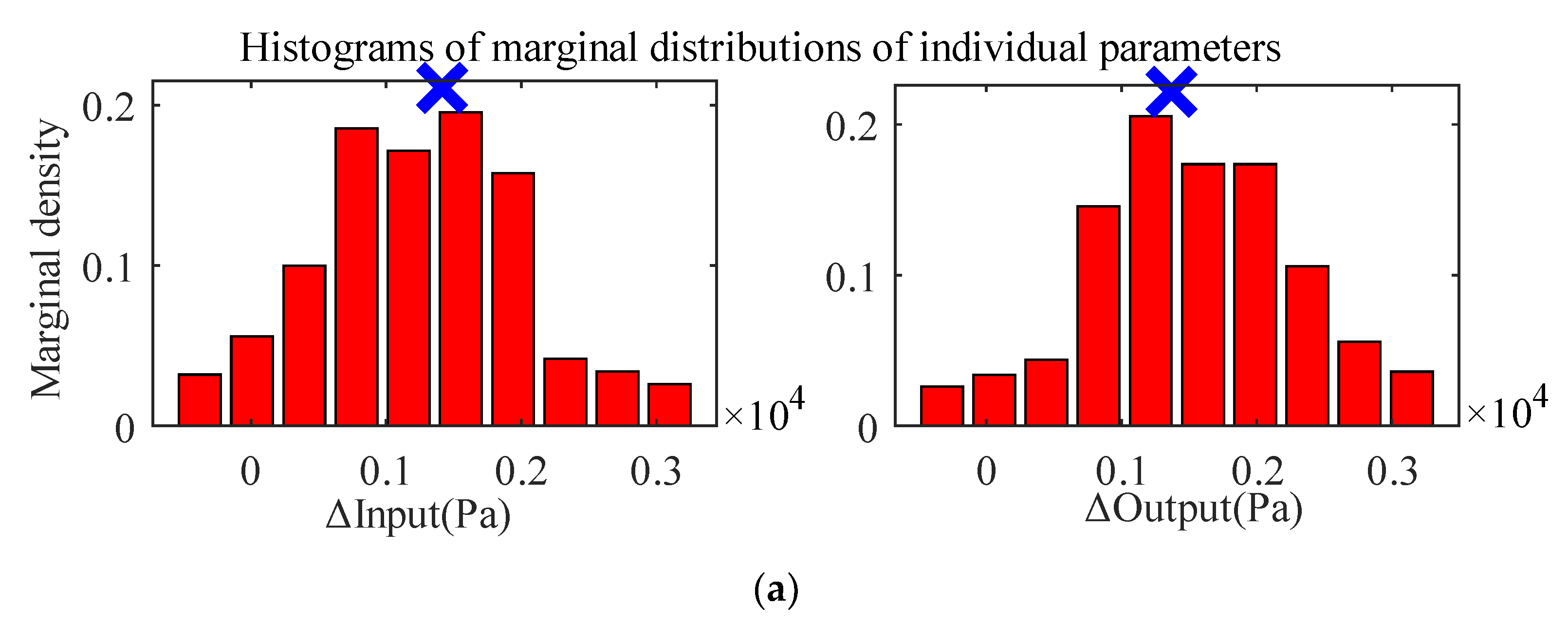
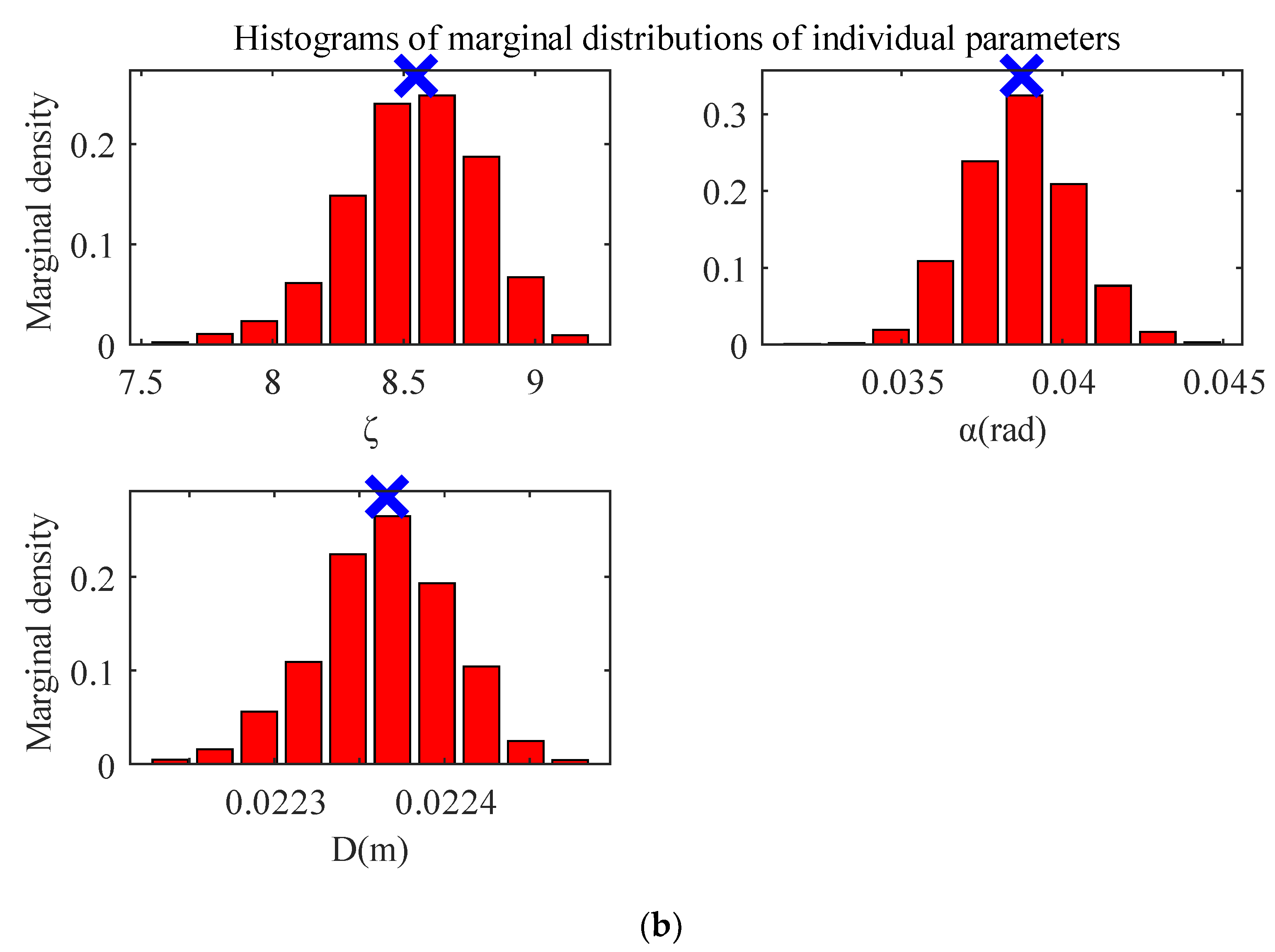
| Parameter | Prior Uncertainty Distribution | Parameter Value at Maximum Posterior Probability |
|---|---|---|
| Input error (Δ Input (Pa) × 104) | N (0, 0.1) | −0.1414 |
| Output error (Δ Output (Pa) × 104) | N (0, 0.1) | −0.137 |
| Coefficient of local resistance (ζ) | N (9, 0.4) | 8.547 |
| Angle (α(rad)) | N (0.04, 0.002) | 0.03874 |
| Internal diameter (D(m)) | N (0.023, 0.00115) | 0.02237 |
| Detection Method | Leak Size | Accuracy |
|---|---|---|
| Pressure residual | Large | 93.36% |
| Small | 84.94% | |
| Resistance coefficient | Large | 99.34% |
| Small | 96.19% | |
| SVM | Large | 92.74% |
| Small | 49.96% |
| Leak Point | Leak Size | Pipeline Entry Data | Leak Location Method | Leak Location | Absolute Error |
|---|---|---|---|---|---|
| 1 | Large | 2.64 m/s 2.84 bar | Model (before correction) | 87.55 m | 74.95 m |
| Model (corrected) | 13.20 m | 0.60 m | |||
| NPW | 9.00 m | 3.60 m | |||
| 2.41 m/s 2.41 bar | Model (before correction) | 74.04 m | 61.44 m | ||
| Model (corrected) | 13.77 m | 1.17 m | |||
| NPW | −2.00 m | 14.60 m | |||
| 2.03 m/s 1.73 bar | Model (before correction) | 62.22 m | 49.62 m | ||
| Model (corrected) | 13.08 m | 0.48 m | |||
| NPW | 6.00 m | 6.60 m | |||
| Small | 2.46 m/s 2.41 bar | Model (before correction) | 181.12 m | 168.40 m | |
| Model (corrected) | 15.96 m | 3.36 m | |||
| NPW | −14.00 m | 26.6 m | |||
| 2.37 m/s 2.26 bar | Model (before correction) | 138.61 m | 126.01 m | ||
| Model (corrected) | 13.41 m | 0.81 m | |||
| NPW | 1.00 m | 11.60 m | |||
| 2.72 m/s 2.64 bar | Model (before correction) | 122.33 m | 109.73 | ||
| Model (corrected) | 10.31 m | 2.29 m | |||
| NPW | 20.50 m | 7.9 m | |||
| 2 | Large | 2.75 m/s 2.92 bar | Model (before correction) | 121.40 m | 87.80 m |
| Model (corrected) | 33.39 m | 0.21 m | |||
| NPW | 26.00 m | 7.60 m | |||
| 2.71 m/s 2.84 bar | Model (before correction) | 122.89 m | 89.29 m | ||
| Model (corrected) | 33.61 m | 0.01 m | |||
| NPW | 25.00 m | 8.60 m | |||
| 2.62 m/s 2.67 bar | Model (before correction) | 126.40 m | 92.80 m | ||
| Model (corrected) | 33.07 m | 0.53 m | |||
| NPW | 32.00 m | 1.60 m | |||
| Small | 2.50 m/s 2.18 bar | Model (before correction) | 160.90 m | 127.3 m | |
| Model (corrected) | 31.20 m | 2.40 m | |||
| NPW | 23.00 m | 9.6 m | |||
| 2.81 m/s 2.74 bar | Model (before correction) | 148.11 m | 114.51 m | ||
| Model (corrected) | 36.20 m | 2.60 m | |||
| NPW | 67.00 m | 33.4 m | |||
| 2.88 m/s 2.83 bar | Model (before correction) | 150.32 m | 116.72 m | ||
| Model (corrected) | 32.15 m | 1.45 m | |||
| NPW | 45.00 m | 11.40 m |
Publisher’s Note: MDPI stays neutral with regard to jurisdictional claims in published maps and institutional affiliations. |
© 2022 by the authors. Licensee MDPI, Basel, Switzerland. This article is an open access article distributed under the terms and conditions of the Creative Commons Attribution (CC BY) license (https://creativecommons.org/licenses/by/4.0/).
Share and Cite
Zhou, M.; Xu, Y.; Cui, B.; Hu, Y.; Guo, T.; Cai, Y.; Sun, X. Pipeline Leakage Detection and Localization Using a Reliable Pipeline-Mechanism Model Incorporating a Bayesian Model Updating Approach. Water 2022, 14, 1255. https://doi.org/10.3390/w14081255
Zhou M, Xu Y, Cui B, Hu Y, Guo T, Cai Y, Sun X. Pipeline Leakage Detection and Localization Using a Reliable Pipeline-Mechanism Model Incorporating a Bayesian Model Updating Approach. Water. 2022; 14(8):1255. https://doi.org/10.3390/w14081255
Chicago/Turabian StyleZhou, Mengfei, Yinze Xu, Baihui Cui, Yinchao Hu, Tian Guo, Yijun Cai, and Xiaofang Sun. 2022. "Pipeline Leakage Detection and Localization Using a Reliable Pipeline-Mechanism Model Incorporating a Bayesian Model Updating Approach" Water 14, no. 8: 1255. https://doi.org/10.3390/w14081255