Study of Identification and Classification Models of Urban Black and Odorous Water Based on Field Measurements of Spectral Data

Abstract

Urban Black and Odorous Water (BOW) has become an environmental problem in many cities in China. The use of satellite remote sensing technology to identify BOW is still in its infancy, and there are many problems that need further solutions. In order to monitor BOW by satellite, between 2016 and 2017, the reflectance of remote sensing and some other parameters of 173 samples were collected from multiple field water experiments first. The samples were located at the major BOW in the urban areas of four Chinese cities, and the differences in remote sensing reflectance of severe BOW (SBOW), moderate BOW (MBOW), and general water (GW) were analyzed. Based on field measurements of spectral data, six remote sensing classification or identification models of BOW were compared in terms of their correct identification rate and reliability. The results show that compared with the GW in the study area, the urban BOW has the lowest reflectance. The peaks and valleys were not obvious in the visible band, especially the remote sensing reflectance of heavy BOW, which fluctuated very little in the visible band. Compared with the other five models, the H Index model had the best identification correctness and reliability.

1. Introduction

Urban Black and Odorous Water (BOW) has been described as having abnormal color (black or grey) and unpleasant odor [1,2]. These waters have become the dominant water environmental problem in many cities in China. The information published on the platform “Urban black and odorous water remediation information” indicates that more than 70% of large and medium-sized cities face black and smelly water problems of varying degrees. This has greatly affected environmental quality [3,4]. The deadline for alleviating this environmental quality issue is described in the “Action Plan for Prevention and Control of Water Pollution”, which was issued by the State Council in 2015 [5]. Therefore, it is of critical importance to monitor urban BOW.

Conventional methods, such as data collection, field measurement, and indoor testing and analysis, are usually adopted to identify and monitor BOW. The data points obtained by this method are scattered and do not clearly represent the actual river and urban water quality. Furthermore, these methods are very time and labor-intensive and are costly [6]. With the development of remote sensing technology, the use of satellite remote sensing to monitor the quality of marine and inland waters has the advantages of time traceability and large-scale synchronous measurement compared with conventional methods [7,8,9]. Remote sensing technology provides an effective way to monitor BOW.

Compared with the more mature application in inland waters, the use of remote sensing technology in monitoring urban BOW is a more recent development. Based on management requirements, Shen [10] established a remote sensing screening system for urban BOW and proposed several technical requirements for identifying them using remote sensing data. Based on BOW samples in different cities, Cao [11] proposed two methods, saturation and spectral index (H Index method), to identify and validate BOW. Wen [12] proposed and validated five algorithms, including Difference of Black-odorous Water Index (DBWI), Slope of Black-odorous Water Index (SBWI), and Normalized Difference Black-odorous Water Index (NDBWI), to identify urban BOW using high spatial resolution remote sensing data. Yao [13] proposed the Black and Odorous Water Index (BOI) algorithm based on the BOW data in Shenyang and achieved good identification effects. Li [14] analyzed the correlation between dissolved organic matter (DOM), apparent optical properties (AOPs), and inherent optical properties (IOPs) of urban BOW and compared it with that of general water (non-BOW water). Jin [15] used GF-2 satellite images to obtain the water area range in the built-up area of Beijing and used multiple water quality parameters to distinguish the degree of BOW. Therefore, a series of comprehensive field water experiments were conducted in the Shenyang and Beijing urban areas. Comparing and analyzing the water quality parameters and spectral characteristics differences of severe BOW (SBOW), moderate BOW (MBOW), and general water (GW), a model of Black and Odorous water Classification Index (BOCI) was proposed [16]. Lu [17] examined the BOW in Qinzhou city, Guangxi Province, as an example and combined PlanetScope data with field data to verify five identification BOW methods. Ding [18] studied the urban BOW in four cities: Nanjing, Wuxi, Yangzhou, and Changsha, and constructed a BOW identification and classification algorithm based on the absorption coefficient.

In conclusion, the research mentioned above set the stage for monitoring BOW by remote sensing. However, the algorithms were designed for a specific area, and though they have high accuracy in that area, their applicability to other areas needs to be verified.

In this study, we examined the BOW in four cities: Shenyang, Beijing, Nanjing, and Shenzhen. From the application perspective, we first evaluated the identification accuracy of several BOW identification models using field data. Then, we set different thresholds for each model to classify BOW into two grades: severe and moderate, before evaluating the accuracy of those classifications. Finally, we attempted to determine which model provided the best results and widest applicability.

2. Materials and Methods

2.1. Data Collection and Processing Methods

2.1.1. Urban Black and Odorous Water

In 2016, the Ministry of Housing and Urban–Rural Development of the People’s Republic of China and the Ministry of Ecology and Environment of the People’s Republic of China co-formulated the Guide to the Remediation of Urban Black and Odorous Water (referred to as the “Guide”). The classification index and test method of the SBOW and MBOW in urban areas were stipulated. The index includes Secchi Depth (SD, cm), dissolved oxygen (DO, mg/L), Oxidation-Reduction Potential (ORP, mV), and NH3-N (mg/L) (

Table 1. Distinguishing standard and index determination method of urban BOW.

Standard	MBOW	SBOW	Note
SD (cm)	10 a–25	<10	On-site in situ measurement
DO (mg/L)	0.2–2.0	<0.2	On-site in situ measurement
ORP (mV)	−200–50	<−200	On-site in situ measurement
NH3-N (mg/L)	8.0–15	>15	Water sample was measured after 0.45 μm filtering

^a When the water depth of the river section was less than 25 cm, we used 40% of the water depth.

).

This study determined the water body type and black and odorous water type based on the criteria in the “Guide” and the results of the field identification of the BOW. Manual identification in the field primarily distinguished BOW according to multiple conditions, such as the color and odor of the water body (

Table 2. Artificial discrimination index of BOW in the field.

Characteristics	Definition	Note
Color	Unnatural color	General water is mainly light green or green
Odor	Unpleasant odor	Severe BOW odor is pungent and nausea-inducing
Fluid Dynamics	Insufficient Hydrodynamic Fluidity	General water is more fluid
Water Body Characteristics	Turbid Water	General water is clearer
Water Surface Characteristics	Industrial or domestic garbage, sludge, and other substances floating on the surface	General water surfaces are cleaner with fewer impurities

).

2.1.2. Remote Sensing Reflectance

An ASD portable spectrometer (ASD, Malvern Panalytical, UK) was used in the field to measure the remote sensing reflectivity of the water surface. The instrument has a spectral resolution of 1 nm and a spectral measurement range of 350–2500 nm. It can obtain continuous water surface spectral data in a study area. The remote sensing reflectance was obtained using the method proposed by Tang et al. (the above-water method) [19]. The spectrometer was preheated and calibrated before each experiment.

The Savitzky–Golay filter model was selected to smooth the measured remote sensing reflectivity of the water body and correct the “jagged edges” phenomenon caused by the influence of external environmental noise during the measurement process [20]. This study used a quadratic polynomial model for smoothing and a window size of 25. Then, using the GF2-PMS2 sensor as an example, the continuous hyperspectral remote sensing reflectance data measured in the field were converted into the GF2-PMS2 sensor band equivalent multispectral data such as 485 nm, 555 nm, 660 nm, and 830 nm. The model algorithm was used to identify BOW from sufficiently sized bodies of water, such as rivers that are wider than 5 pixels.

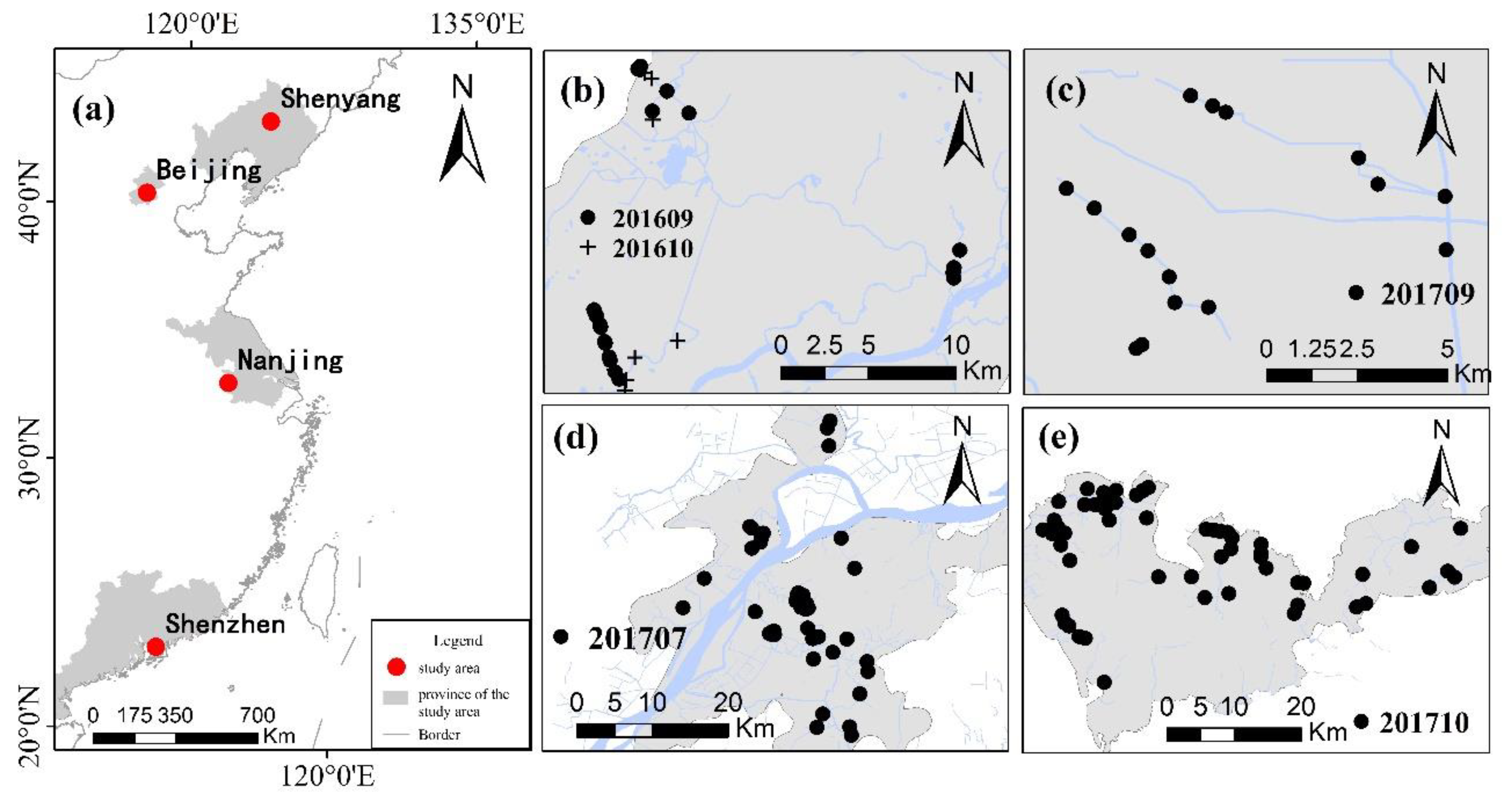
2.2. Study Area and Distribution of Sampling Points

From 2016 to 2017, on sunny days, field experiments were conducted in the urban areas of Beijing, Shenyang, Nanjing, and Shenzhen. The sampling points were distributed in typical cities in Northeast, North, East, and South China and mainly located at rivers and lakes. Some parameters, such as surface remote sensing reflectance and transparency, were measured at each sampling point. Upon collection, water samples were immediately stored in cold storage prior to being transported to the laboratory for analysis of water quality parameters such as ammonia nitrogen. Combining the value of SD, DO, ORP, and NH3-N and on-site artificial sensory identification, the water at each point were classified as SBOW, MBOW, or GW, by the criteria listed in Table 1 and Table 2. Figure 1 shows the geographic location and distribution of sample points in the study area, and

Table 3. Date and number of sampling points.

City	Date	Number of Samples	Number of BOW Samples (SBOW, MBOW)
Shenyang	19 and 20 September 2016	28	25 (25, 0)
Shenyang	9–11 October 2016	28	28 (5, 11)
Beijing	20 September 2017	16	13 (10, 2)
Nanjing	19 and 20 July 2017	53	20 (4, 8)
Shenzhen	19, 20, 22, and 23 October 2017	48	48 (34, 25)
Total	-	173	134 (88, 46)

lists the sampling time and number of samples.

2.3. Remote Sensing Identification Method for Black and Odorous Water

In this study, two classification models, the H Index method and the saturation method, and the four identification models of BOI, SBWI, DBWI, and NDBWI, were selected for the extraction of BOW bodies. The threshold was determined based on the measured data. The GW, SBOW, and MBOW were identified.

2.3.1. The H Index Method

$$H=\frac{2(Rrs(555)-Rrs(485)-Rrs(660))\cdot 345}{sum(Rrs(485):Rrs(830))}\le T$$

(1)

where $Rrs(485)$, $Rrs(555)$, $Rrs(660)$, and $Rrs(830)$ represent the field measured spectral reflectance values corresponding to 485 nm, 555 nm, 660 nm, and 830 nm, respectively. T is the selected threshold.

2.3.2. The Excitation Purity (Pe) Method

The excitation purity (purity for short) of a stimulus is the distance from the white point of the illuminant to the farthest point on the chromaticity diagram at an identical dominant wavelength in the monochromatic sources. CIE (Commission Internationale de l’éclairage, International Commission on Illumination) chromaticity diagram and the purity of point C, which is defined as the distance ratio, i.e., SC/SD. The “white” point S is located at (xs, ys) = (1/3, 1/3). Point C is located at the (x, y) coordinates of a specific R_rs. Point D is the intersection of line SC with the boundary (the spectrum locus) [21]. When the ratio was less than β, a sample was classified as black and odorous water, and when the ratio was greater than β, it was classified as general water.

2.3.3. The BOI Method

$$BOI=\frac{Rrs(G)-Rrs(R)}{Rrs(B)+Rrs(G)+Rrs(R)}\le T,$$

(2)

where $Rrs(B)$, $Rrs(G)$, and $Rrs(R)$ represent the sensing reflectance of the equivalent blue, green, and red bands after remote sensor equivalencing, respectively, and T is the selected threshold.

2.3.4. The SBWI Method

$$SBWI=\frac{\left|Rrs(G)-Rrs(B)\right|}{\Delta {\lambda }_1}\cdot \frac{\left|Rrs(G)-Rrs(R)\right|}{\Delta {\lambda }_2}\le T,$$

(3)

where $Rrs(B)$, $Rrs(G)$, and $Rrs(R)$ represent the sensing reflectance of the blue, green, and red bands after remote sensor equivalencing, respectively; T is the selected threshold; and $\Delta {\lambda }_1$ and $\Delta {\lambda }_2$ represent the difference between the equivalent blue–green and green–red wavelengths on the satellite sensor.

2.3.5. The DBWI Method

$$DBWI=Rrs(G)-Rrs(B)\le T,$$

(4)

where $Rrs(B)$ and $Rrs(G)$ represent the sensing reflectance of the blue and green bands after remote sensor equivalencing, respectively, and T is the selected threshold.

2.3.6. The NDBWI Method

$$NDBWI=\frac{Rrs(G)-Rrs(R)}{Rrs(G)+Rrs(R)}\le T,$$

(5)

where $Rrs(G)$ and $Rrs(R)$ represent the sensing reflectance of the green and red bands after remote sensor equivalencing, respectively, and T is the selected threshold.

2.4. Identification Accuracy Evaluation of Black and Odorous Water

We divided 173 samples of GW, MBOW, and SBOW in the study area into two parts by a 1:2 ratio, namely, the threshold selection sample and the accuracy verification sample. Two-thirds of the samples (115) were used to select the appropriate model thresholds, and the remaining one-third of the samples (58) were used to evaluate the accuracy of the model. This study used identification accuracy (RA) for accuracy verification. The formula is as follows [21]:

$$RA=\frac{M}{N}\cdot 100\%$$

(6)

where M represents the number of correctly identified samples in each category and N represents the total number of samples in each category.

To further evaluate the uncertainty and reliability of the BOW water identification model, we used the overall classification accuracy (OA) and KAPPA coefficients to evaluate the quantitative classification accuracy [22,23,24].

3. Results

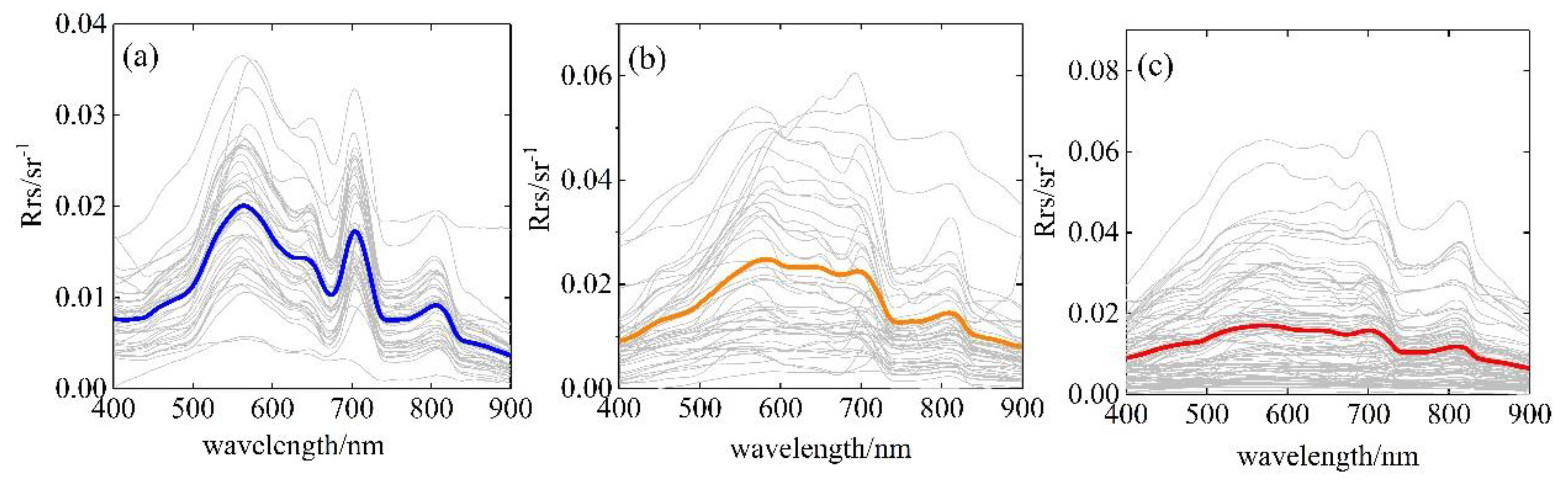
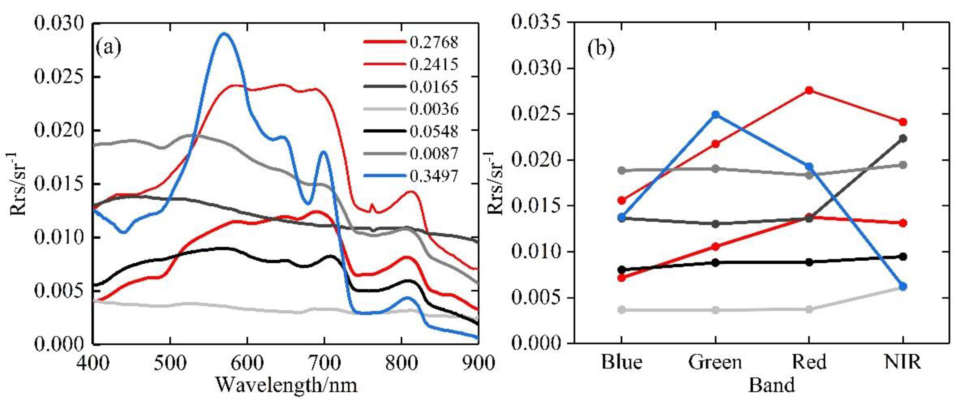
3.1. Spectra Characteristics of Black and Odorous Water Bodies

The difference in the spectral characteristics between the SBOW, MBOW, and the GW in the study area were analyzed (Figure 2). Generally, because of the absorption of chlorophyll a and phycocyanin, the water reflectance valleys appeared near the three wavebands of 440 nm, 620 nm, and 675 nm, with the peaks near the three wavebands of 550 nm, 650 nm, and 700 nm. According to the measured water quality parameters in this study, the chlorophyll a concentration of general water (100.62 mg/m³) is considerably higher than that of black and odorous water (MBOW: 1.84 mg/m³; SBOW: 2.55 mg/m³), the reflectance peak of the red band at 700 nm was higher. Compared with GW, the change is slow for SBOW in the range of 500–700 nm, without obvious peaks and valleys. MBOW had a remote sensing reflectance similar to GW in the 400–550 nm and 700–900 nm wavebands, but the reflectance fluctuations in the 550–700 nm range were relatively small.

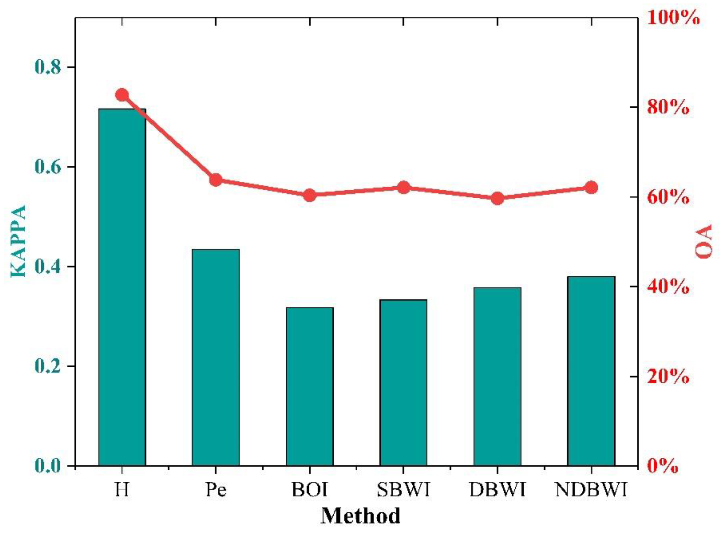
3.2. Evaluation and Comparison of Algorithm Identification Accuracy Based on Measured Spectra

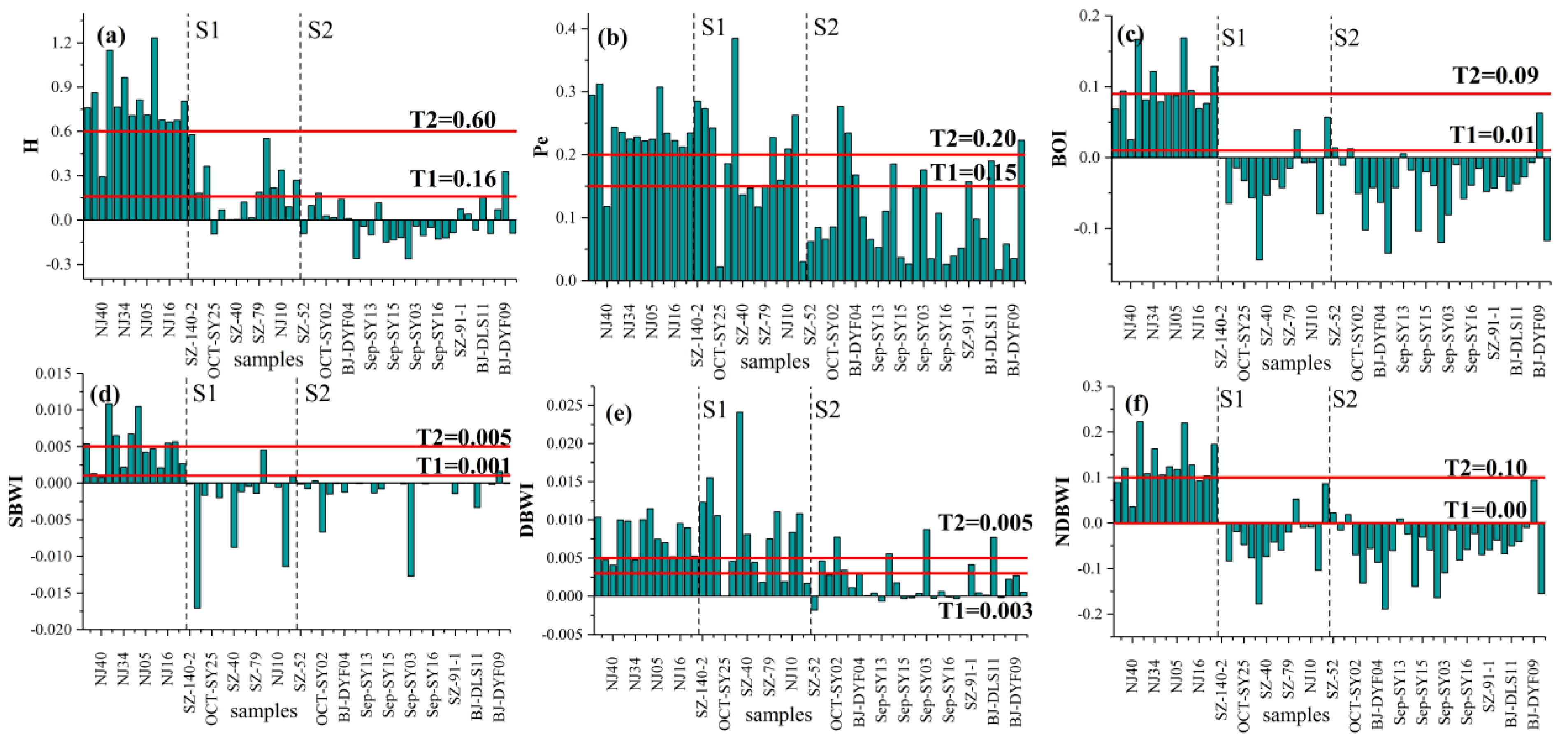
3.2.1. Threshold Determination

The satellite sensor equivalent waveband reflectance data measured at 116 sampling points in the study area (GW: 25, MBOW: 31, and SBOW: 60) were input into the six models, and thresholds were chosen for each model. As shown in Figure 3, the ordinate represents the frequency histogram of the three water classifications as calculated by a model. The blue, yellow, and dark gray columns represent GW, MBOW, and SBOW, respectively. The thresholds used to distinguish the three water types were determined based on the distribution of the frequency histograms. By taking the H model as an example, the frequency histogram shows that 92% of GW samples had an H > 0.6, and 87% of the MBOW had an H < 0.6. Therefore, T₂ = 0.60 was used to distinguish MBOW from general water samples. Additionally, 93.22% of the SBOW had an H < 0.16, and 90.32% of MBOW had an H > 0.16. Therefore, T₁ = 0.16 was used as the threshold to distinguish MBOW from SBOW. The thresholds of each model were determined in a similar fashion. The thresholds to identify GW, MBOW, and SBOW were the following. Pe: T₁ = 0.15, T₂ = 0.20; BOI: T₁ = 0.04, T₂ = 0.09; SBWI: T₁ = 0.001, T₂ = 0.005; DBWI: T₁ = 0.003, T₂ = 0.005; and NDBWI: T₁ = 0.00, T₂ = 0.10.

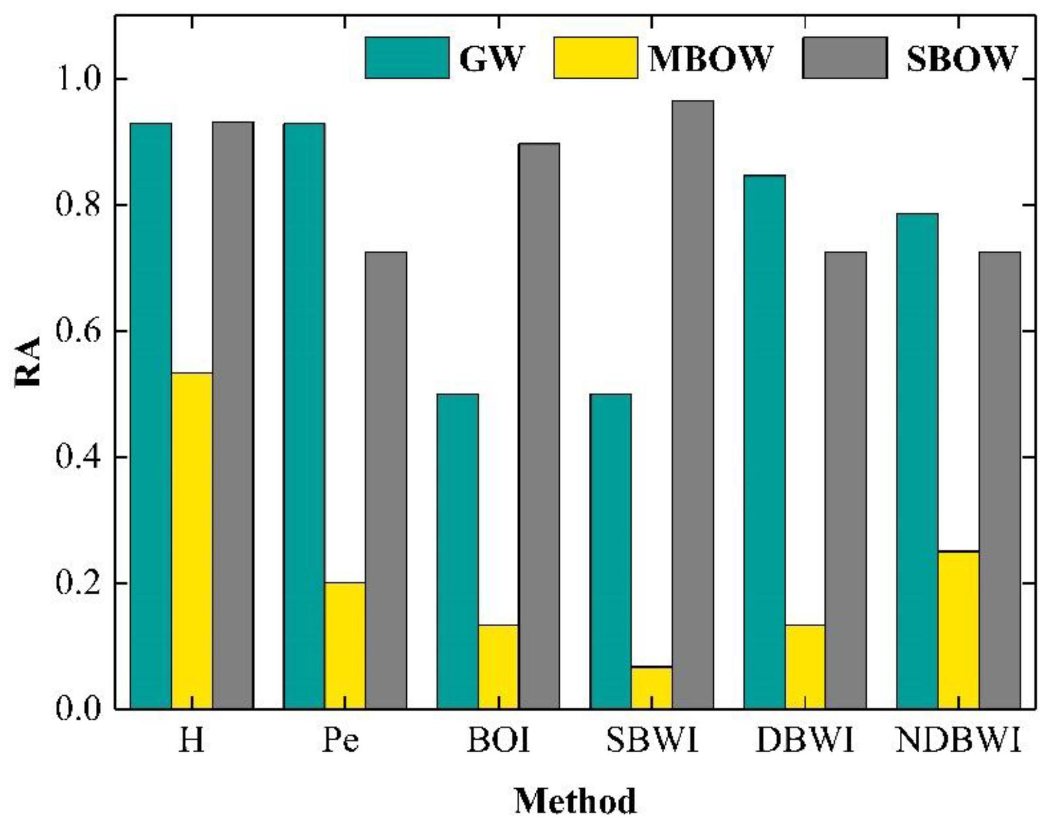
3.2.2. Accuracy Evaluation

The 58 measured spectrum data (GW: 14; MBOW: 15; and SBOW: 29) were input into the six models, and the thresholds of each model determined in the previous step were used to verify the accuracy of the identification results. As shown in Figure 4 and Figure 5, for the H model, only one of the 14 GW samples was misclassified, and the identification accuracy was as high as 92.86%. All 44 BOW samples were identified successfully. Of the 15 MBOW samples, eight were correctly recognized, with an identification accuracy of 53.33%. Only 2 of the 29 SBOW samples were recognized incorrectly, with an identification accuracy as high as 93.10%. The identification accuracy of the GW of the Pe method was consistent with the H index method (92.86%), and the identification accuracy of BOW was 59.10%. Among them, the SBOW identification accuracy was slightly lower (72.41%), and the MBOW identification accuracy was only 20%. The SBWI method had high accuracy in recognizing BOW samples (95.45%), among which the SBOW identification accuracy was the highest (96.55%). However, the identification accuracy of GW and MBOW was very low, with MBOW at only 6.67%. The identification results of the BOI model and the SBWI model were consistent. The accuracy of the NDBWI and DBWI methods for recognizing BOW samples were 86.36% and 56.82%, respectively. Among them, the identification accuracy of SBOW was 72.41%, and the identification accuracy of GW was 78.57%.

In summary, among the six BOW identification methods, only the H index model had an accuracy greater than 50% for recognizing MBOW, and the identification rate for both mild and severe BOW was higher than 80%. This was the best overall identification accuracy.

To further quantitatively evaluate the uncertainty and reliability of the BOW identification models, this study used the OA and KAPPA coefficients to evaluate the classification accuracy. As shown in Figure 6, the KAPPA coefficient of the H index method was the highest among the six models, followed by the Pe method. The KAPPA coefficients of the remaining identification algorithms were all less than 0.4, which means that the consistency of the classification results was average. From the perspective of the OA, the H index model had the highest (82.76%), and its overall identification effect was the best. The OA of the other models was around 60%.

Compared with other identification algorithms, the H-index model had the highest identification accuracy and reliability. This model can be used to effectively identify BOW and classify them into two levels of severity.

4. Discussion

Section 3.2 evaluates the identification accuracy of different algorithms. All models had a high identification accuracy for GW and SBOW, but the identification accuracy for MBOW was very low. Among them, only the H index model had an identification accuracy greater than 50% for MBOW. In addition, the Pe and DBWI models tended to misidentify some BOW as GW. The SBWI method tended to identify GW as BOW. The main reasons for the above phenomenon are described below:

The remote sensing reflectance of some measured MBOW in the study area was comparable to GW or SBOW. After wave band equivalencing, the hyperspectral remote sensing reflectance was converted to multispectral remote sensing reflectance, making the difference smaller, and thus lowering the identification accuracy rate of the MBOW.

Using the Pe model as an example (Figure 7), the gray curve has no obvious changes in the near-infrared band, and it can directly be classified as BOW using the Pe method. However, for example, the red curve and the blue curve in Figure 7 vary greatly in the visible light band. The remote sensing reflectance of these BOW samples exhibited the reflectance characteristics of GW. After satellite sensor band equivalencing, the visible light retained considerable variation. As a result, the calculated purity was misrecognized as a GW (the calculated purity of the samples of the two red curves was greater than 0.2).

The instrument measurement errors and the human intuitive perception of BOW, which misidentified the types of water in the field measurement process, ultimately affected the identification accuracy of the model.

5. Conclusions

Compared with GW in the study area, in the range of 500–700 nm, the overall remote sensing reflectance fluctuations of SBOW were relatively small. MBOW were similar to GW in the two wavebands of 400–550 nm and 700–900 nm, but the reflectance fluctuations of MBOW in the 550–700 nm range were relatively small, which is different from GW.

By using the field measurement data in the study area, six typical BOW remote sensing identification models were compared. The results show that the H Index model was more effective in terms of identification accuracy and model reliability.

The next step of the research will be to explore the factors affecting the identification accuracy of BOW and classify the remote sensing reflectance of mild and severe BOW and GW in more detail based on the characteristics of BOW. Additionally, efforts will be directed toward selecting appropriate identification models for various categories to obtain higher identification accuracy.

Future research should use multi-source high spatial resolution remote sensing images to develop better identification models, extract the temporal and spatial distribution of BOW in the study area, and monitor the changes in urban BOW pollution levels in real time. This will provide technical support for government agencies to scientifically and effectively rectify and supervise urban BOW. We will attempt to apply this method to the supervision of black and odorous water in rural areas.

References

1. Wen, S.; Wang, Q.; Li, Y.M.; Zhu, L.; Lv, H.; Lei, S.H.; Ding, X.L.; Miao, S. Remote Sensing Identification of Urban Black-Odor Water Bodies Based on High-Resolution Images: A Case Study in Nanjing. Environ. Sci. 2018, 39, 57–67. [Google Scholar]
2. Yao, Y.; Shen, Q.; Zhu, L.; Gao, H.J.; Cao, H.Y.; Han, H.; Sun, J.G.; Li, J.S. Remote sensing identification of urban black-odor water bodies in Shenyang city based on GF-2 image. J. Remote Sens. 2019, 23, 230–242. [Google Scholar]
3. Ding, X.L.; Li, Y.M.; Lv, H.; Zhu, L.; Wen, S.; Lei, S.H. Analysis of Absorption Characteristics of Urban Black- odor Water. Environ. Sci. 2018, 39, 4519–4529. [Google Scholar]
4. Yang, H.F. Study on the Main Influencing Factors and Comparative Treatment Case of Black and Foul Water Pollution in Shanghai City. Master’s Thesis, Shanghai Normal University, Shanghai, China, 2007. [Google Scholar]
5. Wang, X.; Wang, Y.G.; Sun, C.H.; Pan, T. Formation mechanism and assessment method for urban black and odorous water body: A review. Chin. J. Appl. Ecol. 2016, 27, 1331–1340. [Google Scholar]
6. Li, J.Q.; Li, J.G.; Zhu, L.; Shen, Q.; Dai, H.Y.; Zhu, Y.F. Remote sensing identification and validation of urban black and odorous water in Taiyuan city. J. Remote Sens. 2019, 23, 773–784. [Google Scholar]
7. Zhu, L.; Li, Y.M.; Zhao, S.H.; Guo, Y.L. Remote sensing monitoring of Taihu Lake water quality by using CF-1 satellite WFV data. Remote Sens. Land Resour. 2015, 27, 113–120. [Google Scholar]
8. Chen, Y.; Huang, C.P.; Zhang, L.F.; Qiao, N. Spectral Characteristics Analysis and Remote Sensing Retrieval of COD Concentration. Spectrosc. Spectr. Anal. 2020, 40, 824–830. [Google Scholar]
9. Wu, Y.Q.; Liu, Z.L. Research progress on methods of automatic coastline extraction based on remote sensing images. J. Remote Sens. 2019, 23, 582–602. [Google Scholar]
10. Shen, Q.; Zhu, L.; Cao, H.-Y. Remote sensing monitoring and screening for urban black and odorous water body: A review. Chin. J. Appl. Ecol. 2017, 28, 3433–3439. [Google Scholar]
11. Cao, H.Y. Study on Analysis of Optical Properties and Remote Sensing Identifiable Models of Black and Malodorous Water Study on Analysis of Optical Properties and Remotesensing Identifiable Modelsof Black and Malodorous Water in Typical Cities in China. Master’s Thesis, Southwest Jiaotong University, Chengdu, China, 2017. [Google Scholar]
12. Wen, S. Remote Sensing Recognition of Urban Black and Odorous Water Bodies Basedon GF-2 Images—A Case Study in Nanjing. Master’s Thesis, Nanjing Normal University, Nanjing, China, 2018. [Google Scholar]
13. Yao, Y. Study on Urban Black-odor Water Identification Model Based on Gaofen Multispectral Images. Master’s Thesis, Lanzhou Jiaotong University, Lanzhou, China, 2018. [Google Scholar]
14. Li, X.J. Pollutant Characteristics and Remote Sensingidentification of Typical Black and Odorous Water. Master’s Thesis, Chang’an University, Xi’an, China, 2018. [Google Scholar]
15. Jin, H.X.; Pan, J. Urban Black-Odor Water Body Remote Sensing Monitoring Based on GF-2 Satellite Data Fusion. Sci. Technol. Manag. Land Resour. 2017, 34, 107–117. [Google Scholar]
16. Qi, K.K. Remote Sensing Classification And Recognition Of Urban Black And Odorous Water Based On Multi-Source High-Resolution Images. Master’s Thesis, Southwest Jiaotong University, Chengdu, China, 2019. [Google Scholar]
17. Lu, Y.N. Remote Sensing Recognition And Classificationof Urban Black And Odourous Water Body Basedon Planetscope Images: A Case Study In Qinzhou, Guangxi Province. Master’s Thesis, Guangxi University, Nanning, China, 2019. [Google Scholar]
18. Ding, X.L. Study on Remote Sensing identification and Classification of Urban Black and Odor Water Based on Water Absorption Coefficient. Master’s Thesis, Nanjing Normal University, Nanjing, China, 2019. [Google Scholar]
19. Mueller, J.L.; Fargion, G.S.; McClain, C.R. Special topics in ocean optics protocols. In Ocean Optics Protocols for Satellite Ocean Color Sensor Validation, 5th ed.; NASA: Greenbelt, MD, USA, 2003; pp. 1–36. [Google Scholar]
20. Ruffin, C.; King, R.; Younan, N.H. A Combined Derivative Spectroscopy and Savitzky-Golay Filtering Method for the Analysis of Hyperspectral Data. GIScience Remote Sens. 2008, 45, 1–15. [Google Scholar] [CrossRef]
21. Shen, Q.; Yao, Y.; Li, J.S.; Zhang, F.F.; Wang, S.L.; Wu, Y.H.; Ye, H.P.; Zhang, B. A CIE Color Purity Algorithm to Detect Black and Odorous Water in Urban Rivers Using High-Resolution Multispectral Remote Sensing Images. IEEE Trans. Geosci. Remote Sens. 2019, 57, 6577–6590. [Google Scholar] [CrossRef]
22. Yang, F.; Wang, B. Research of Remote Sensing Image Classification Based on Decision Tree Method. Geomat. Spat. Inf. Technol. 2019, 42, 1–4. [Google Scholar]
23. Xu, Z.Y.; Luo, Q.H.; Xu, Z.L. Consistency of Land Cover Data Derived from Remote Sensing in Xinjiang. J. Geo.-Inf. Sci. 2019, 21, 427–436. [Google Scholar]
24. Zhao, R.; Su, X.K.; She, W.Q.; Xu, K.F.; Wei, M.Y. Remote sensing monitoring of Dongting Wetland information based on LANDSAT Time Series Data. Environ. Dev. 2019, 31, 128–131. [Google Scholar]
Figure 1. Study area and distribution of sampling points. (a): geographical distribution of the study area; (be): grey areas represent the urban areas of Shenyang, Beijing, Nanjing, and Shenzhen city, respectively; blue indicates urban rivers.
Water 14 01254 g001
Figure 2. Remote sensing reflectance of BOW and GW: (a) GW; (b) MBOW; and (c) SBOW. The blue, orange, and red curves represent the average reflectance values of GW, MBOW, and SBOW between 400 and 900 nm, respectively.
Water 14 01254 g002
Figure 3. Model threshold determination. The two red lines show the threshold values between GW, MBOW, and SBOW. The center line of the light gray column (light BOW) was taken as the model extraction result corresponding to the horizontal axis. (af): the frequency distribution histogram of six kinds of BOW identification models: H index, Pe, BOI, SBWI, DBWI, and NDBWI, respectively.
Water 14 01254 g003
Figure 4. Model accuracy verification and comparison. (af) represent the accuracy verification results of H index, Pe, BOI, SBWI, DBWI, and NDBWI, respectively. Two red lines, T1 and T2, represent the thresholds determined by each model (distinguishing GW, MBOW, and SBOW). Two black dashed lines, S1 and S2, represent the boundaries of GW, MBOW, and SBOW, respectively.
Water 14 01254 g004
Figure 5. Identification accuracy of models.
Water 14 01254 g005
Figure 6. Model accuracy verification by overall accuracy and KAPPA coefficient.
Water 14 01254 g006
Figure 7. Spectral curve comparison. (a) The figures in the legend show the Pe determined according to the remote sensing reflectance. Two red curves show that the Pe of the water with SBOW was mistakenly recognized as a GW. The four black curves show that the Pe of the water with SBOW remained classified as SBOW after calculation, and the blue curve shows a GW. (b) The remote sensing reflectance after the equivalent band of the satellite sensor corresponding to (a).
Water 14 01254 g007