
Numerical Simulation of the Trajectory of Garbage Falling into the Sea at the Coastal Landfill in Northeast Taiwan


1
Department of Marine Environmental Informatics, National Taiwan Ocean University, 2 Pei-Ning Road, Keelung 202301, Taiwan
2
Environmental Protection Administration, 83, Sec. 1, Zhonghua Road, Taipei 100006, Taiwan
3
Department of Earth Science, National Taiwan Normal University, 88, Sec. 4, Tingzhou Road, Taipei 116059, Taiwan
4
Department of Political Science, National Cheng Kung University, 1 University Road, Tainan 701401, Taiwan
*
Author to whom correspondence should be addressed.
Water 2022, 14(8), 1251; https://doi.org/10.3390/w14081251
Submission received: 9 March 2022
/
Revised: 8 April 2022
/
Accepted: 11 April 2022
/
Published: 13 April 2022
(This article belongs to the Special Issue Marine Environmental Research)
Abstract
:This study used a numerical model to simulate the floating trajectory of garbage falling into the sea from the landfill near the coast of Wanghaixiang Bay in northeast Taiwan to understand its impact on the local environment. The Regional Ocean Model System was used to simulate the probability densities of the distribution of garbage drifting trajectories under scenarios of no-wind, northeast monsoon, and typhoons. The results show that, in the no-wind scenario, garbage was mainly affected by tidal currents. It moved in the northwest–southeast direction outside the bay. In the northeast monsoon scenario, garbage was forced toward the shore due to the windage effect. In typhoon scenarios, strong winds forced the garbage to the shore, as typhoons continued to advance and the wind direction kept changing, the garbage trajectory was also changed. After typhoons moved away, the drifting trajectory of the garbage was again affected by tidal currents. When the garbage falling into the sea was located in the bay or the mouth of the bay, the garbage had a higher probability of being forced into the bay by typhoons.
1. Introduction
Marine garbage has been an important issue because it presents a series of adverse effects on the environment and economy. To understand the floating situation of marine garbage, many studies have used satellite remote sensing or drones to find floating marine debris or its traces, and some have used numerical models to simulate drifting conditions [1]. For example, satellite-derived sea surface height and wind stress to determine surface circulation were used to calculate the trajectory of floating garbage [2]. To maintain the observation of marine plastic debris on a global scale, a satellite remote sensing system was designed that can determine the characteristics of marine plastic debris and emphasize its oceanic processes [3]. The ability to use satellite sensors to detect marine debris in the bay was also demonstrated [4]. For the coastal area, unmanned aerial vehicles (UAVs) can be a useful tool to monitor marine garbage in protected area [5].
Numerical modeling is an effective tool for simulating the trajectory of floating garbage in the ocean and can provide a deeper understanding of the distribution of marine litter. In recent years, numerical models of various complexity levels have been used to simulate the drift of marine debris [6,7,8]. Their results were used to formulate strategies to reduce marine garbage. For example, two plastic bottles in the Coral Sea of the Southwest Pacific were simulated their navigation using a numerical model [9]. Their result showed that not only ocean currents, but also mesoscale and sub-mesoscale activities, can affect the drift of marine debris. A particle-tracking model was developed to study floating garbage transport in Iberian waters [10]. It was found that the wind drag coefficient changes depending on the wind direction and the drifter position. In addition, a marine debris monitoring system combining numerical modeling simulation and satellite remote sensing technology was proposed [11]. The system used remote sensing images to provide spatial coverage and consistent measurement time series from local to global scales, and used numerical models to optimize system design and gradually improve system products.
The origin of marine debris can be divided into sea-based and land-based input. Sea-based origin refers to litter that is released directly into the sea by maritime activities. One of the land-based sources is landfills [12]. Coastal landfills are a way of solving the problem of garbage, especially in countries with limited living areas. To prevent coastal landfills from polluting the sea area, seawalls are usually built to protect them. If not properly maintained, these can be damaged by flooding and/or erosion [13], which can be caused by storms and rising sea level [14,15]. When the seawall is damaged and buried garbage flows into the sea, floating marine debris poses a serious threat to the marine ecosystem.
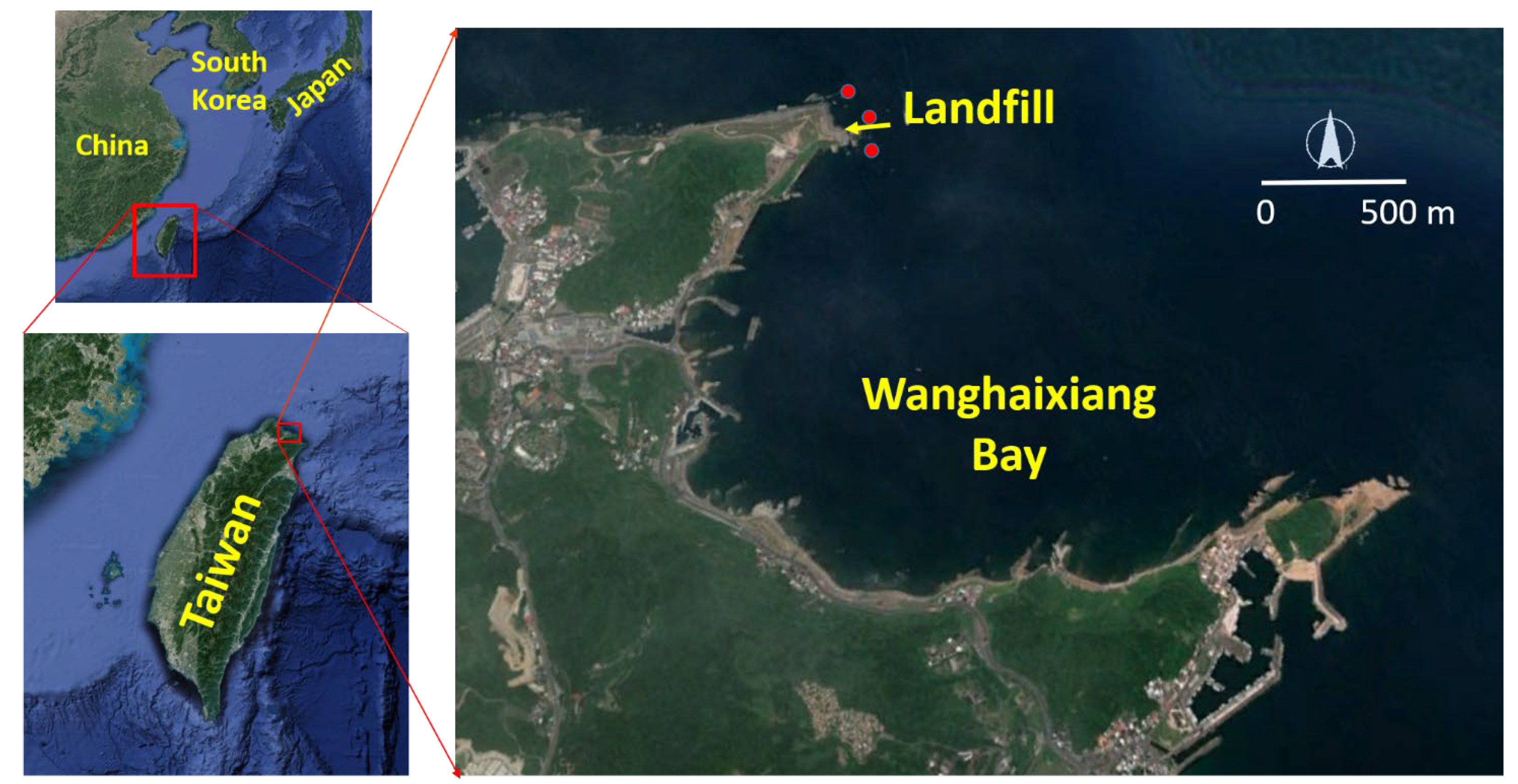
Taiwan is a small island located in East Asia, with a north–south mountain range in the center. It has a limited living area and is one of the highest population densities in the world. To dispose of garbage, some coastal landfills have been built, one of which is located in the north corner of Wanghaixiang Bay (Figure 1) in Keelung. Keelung is a city located at the northern tip of Taiwan, facing the East China Sea to the north. The landfill was opened in 1976 and closed in 1992. The total area is approximately 10 hectares, the total volume is approximately 1.55 million cubic meters, the total weight is approximately 2.24 million tons, and the burial depth is approximately 15 m. As the landfill was built by the sea, the landfill dam was built at the forefront of the wave cutting platform, which was extremely vulnerable to the impact and erosion of waves. The area is usually affected by typhoons in summer and northeast monsoons in winter. The seawalls on the north and east sides are easily damaged. In recent years, the seawalls have collapsed twice, which caused the buried garbage to be exposed (Figure 2) and flow into the ocean, polluting the marine environment.
The area of Wanghaixiang Bay is approximately 250 hectares and the distance between its north and east caps is approximately 2.2 km. It is rich in marine ecology and has been favored by tourists in recent years. It has become a hot spot for underwater activities in Northern Taiwan, with more than 25,000 divers visiting each year. In addition, the bay is also the place in which water lanterns are placed during the Ghost Festival, a folk festival in Keelung. Therefore, the purpose of this study is to understand whether the coastal embankment of this landfill is damaged by waves, how the buried garbage will pollute the bay, or whether it may flow out to the open sea with the current. The study used a numerical model to simulate garbage drift in the bay under strong northeast monsoon waves and typhoon waves passing through northern Taiwan. The research results could provide a reference for the formulation of policy by the relevant units.
2. Environment of Study Area
2.1. Bathymetry
The National Taiwan Marine Science and Technology Museum conducted a water depth survey of Wanghaixiang Bay in October 2014. The survey used a multibeam echo sounder for measurements. The measurement results show that the maximum depth of the bay is approximately 40 m, located at the entrance of the bay, and the average depth of the water of the bay is approximately 25 m.
2.2. Tide
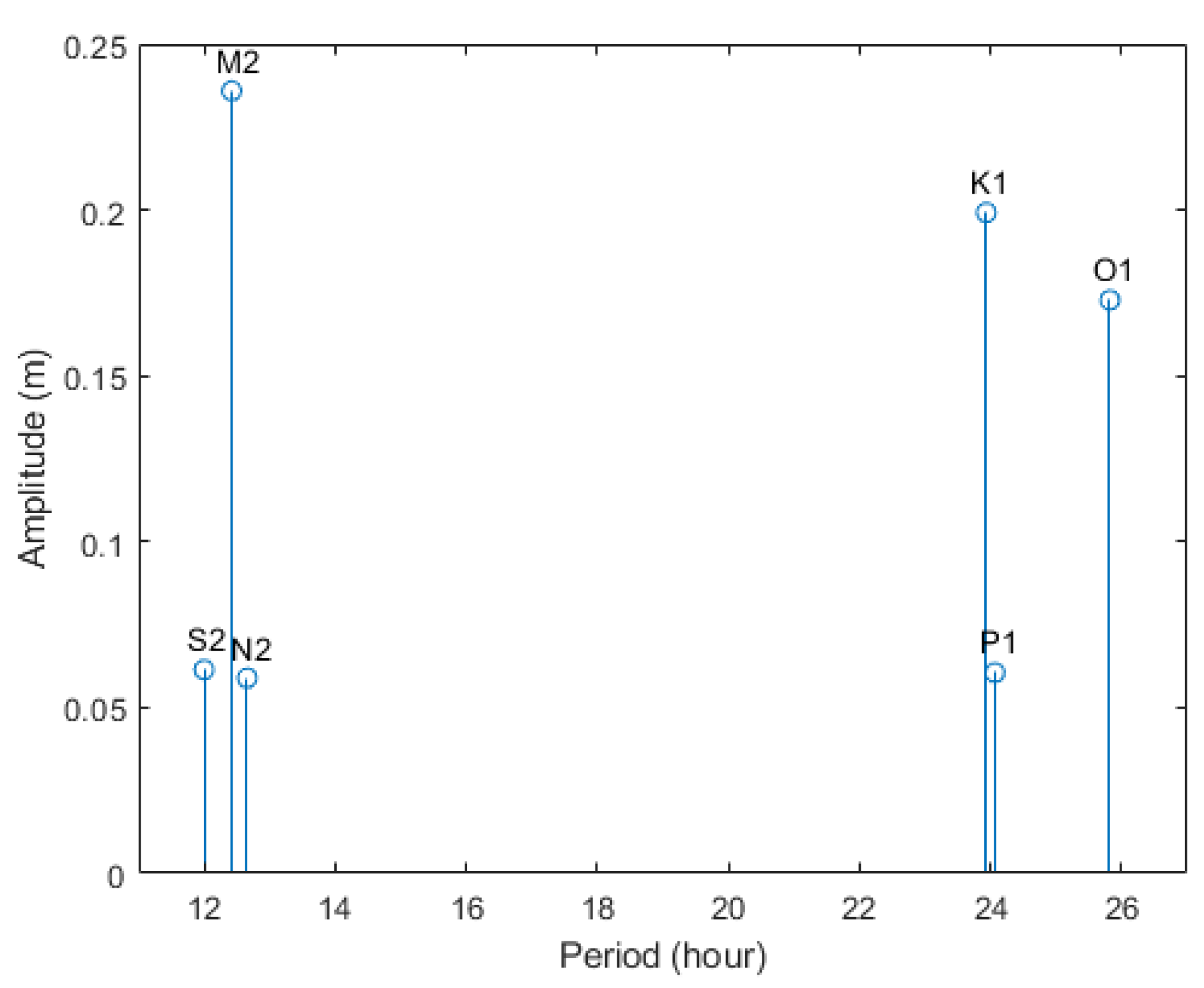
The Keelung tidal station has served as the reference tidal station in Taiwan for more than a century. It contains long-term tide gauge data. The amplitudes of the four main tidal constituents are generally used to classify the tidal type [16]. These are K1 (lunar diurnal constituent), O1 (lunar diurnal constituent), M2 (principal lunar semidiurnal constituent), and S2 (principal solar semidiurnal constituent). The tide is classified as semidiurnal when the ratio of the tidal constituents of (K1 + O1)/(M2 + S2) is less than 0.25; the ratio between 0.25 and 1.5 is classified as mixed, mainly semidiurnal; the ratio between 1.5 and 3.0 is mixed, mainly diurnal; and the ratio is diurnal when the ratio is greater than 3.0. Figure 3 shows six major tidal constituents in Keelung based on the tide gauge data from 2010 to 2019. The constituent ratio is 1.25. According to this classification criterion, it belongs to a mixed tide, mainly semidiurnal. Its tidal range is about 0.5 m on average.
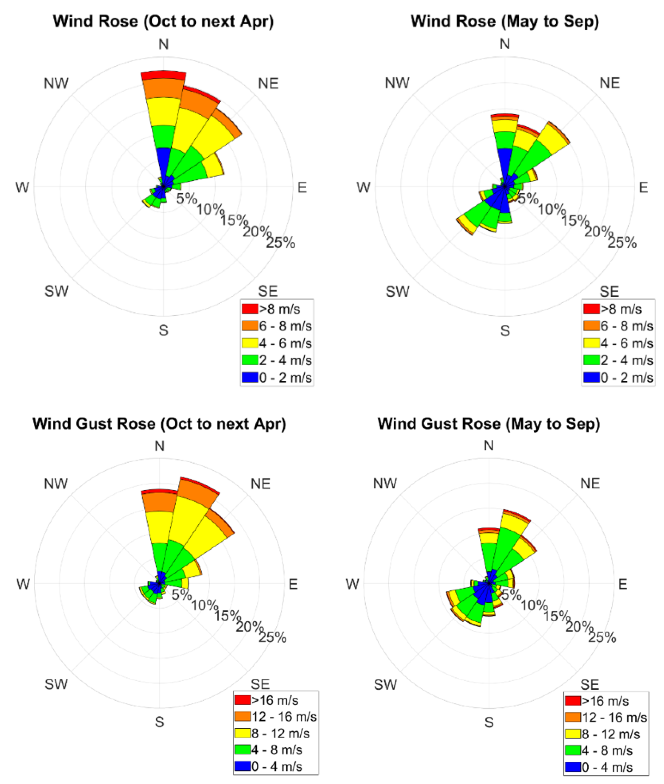
2.3. Monsoon
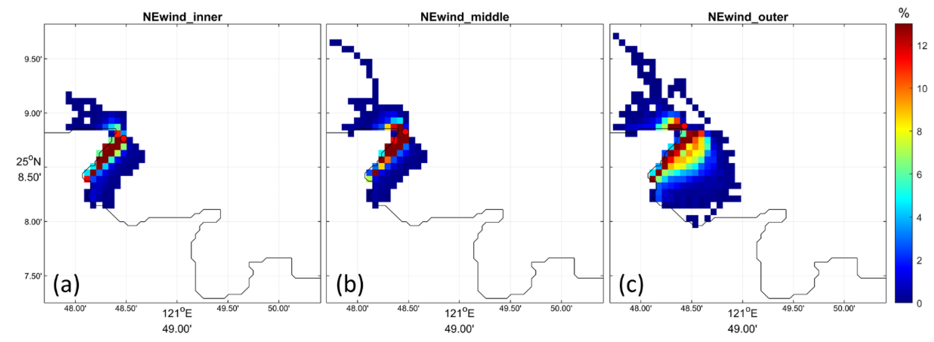
Taiwan is located in the monsoon area of East Asia. Northeast monsoons with gusting winds blow from October to the following April. Southwest monsoons come with a lower wind speed from May to September. According to data collected by the Keelung weather station, Figure 4 shows the wind and gusty wind roses from 2011 to 2020. It is obvious that there are more and stronger north wind than south wind from October to next April, regardless of wind or wind gust. The percentage of south wind increases, but is still lower than that of the north wind from May to September. About 10.8% of the winds have wind speeds higher than 6 m/s, and 10.7% of the wind gusts have wind speeds higher than 12 m/s during the northeast monsoon season.
2.4. Typhoon
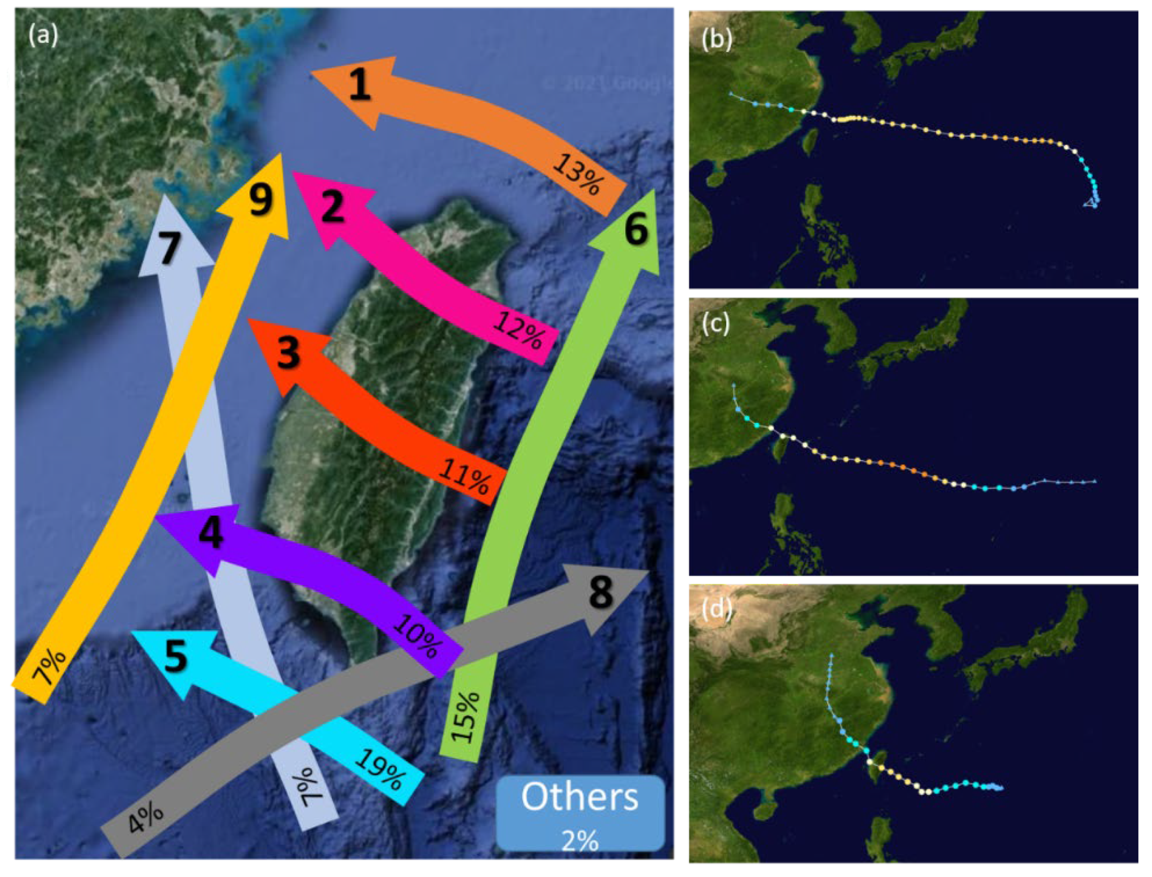
Typhoons usually invade Taiwan from June to October, with August and September having more frequent typhoons. An average of 3.5 typhoons hit Taiwan every year, causing heavy rainfall and environmental damage. According to statistics from Taiwan’s Central Weather Bureau, there are nine routes for typhoons to hit Taiwan (Figure 5a), but those crossing northern Taiwan (Route 2) and the sea off the north coast (Route 1) usually cause the most damage. As shown in Figure 5a, about 58% of the typhoons (Routes 1, 2, and 3) may directly affect Keelung. In this study, the effects of garbage drifts during three typhoon scenarios were simulated by a numerical model. Typhoon Sinlaku (2002) and Typhoon Lekima (2019) passed through the outside of northern Taiwan, i.e., Route 1. Typhoon Soulik (2013) and Typhoon Dujuan (2015) passed through northern Taiwan, i.e., Route 2. Typhoon Fung-Wong (2008) passed through central Taiwan, that is, Route 3. The tracks of the three typhoons are shown in Figure 5b–d. Table 1 shows the typhoon information used in this study.
3. Description and Validation of Model Simulation
The Regional Ocean Modelling System (ROMS), in conjunction with a particle-tracking model, was used to study the distribution of floating garbage in Wanghaixiang Bay. ROMS was widely used in the study of the trajectory of marine garbage. It has been applied to analyze the distribution of floating marine garbage in Iberian [17]. The results show that there is a seasonal variation in the distribution and residence time of marine garbage.
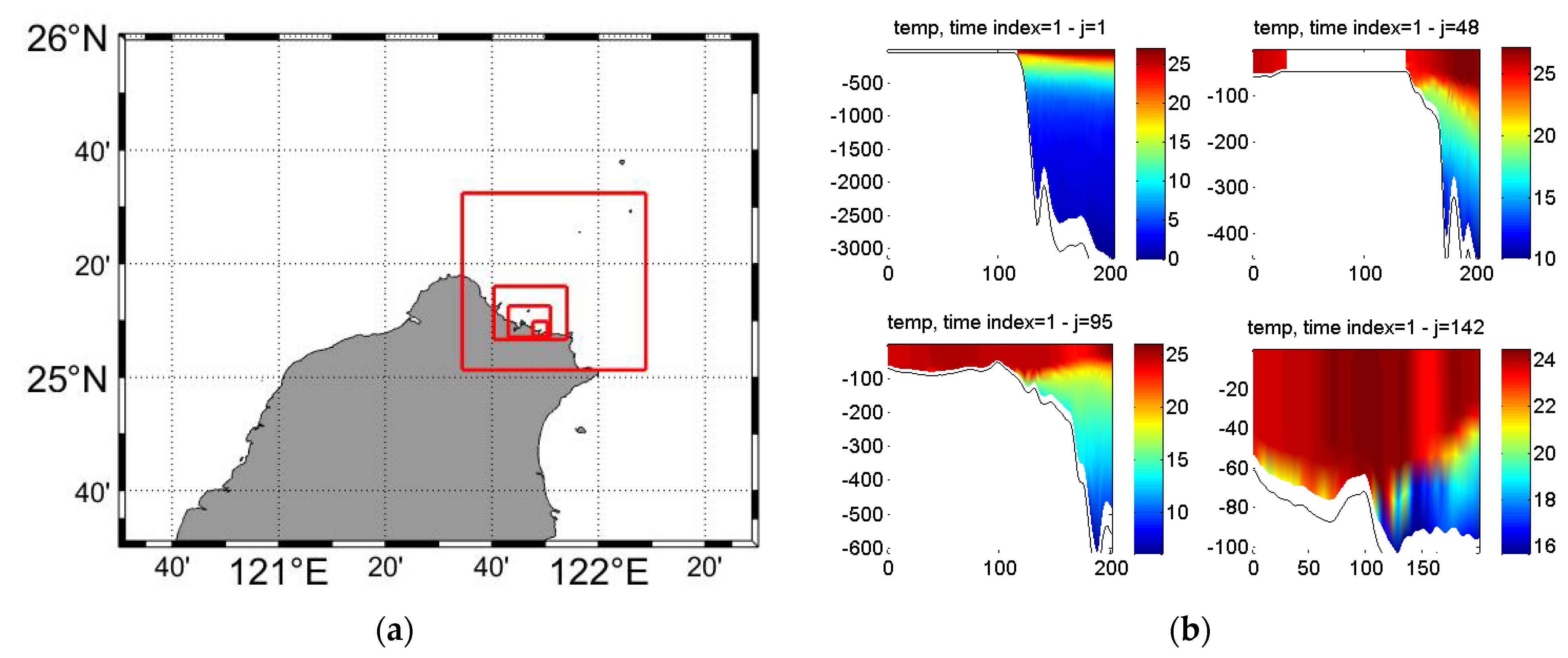
ROMS is an ocean model with free-surface and primitive equations. It has been widely used by the scientific community for surface objective tracking, such as oil transport [18] and floating garbage tracking [17,19]. The ROMS calculation applies the nonlinear kernel [20,21], and the tangent linear and adjoining kernels algorithms [22]. It also includes several vertical mixing schemes [23], and multiple layers of nested and combined grids. Furthermore, to address the difficulties in bridging the gap between near-shore and offshore dynamics, the nesting capability of the 5-layers domain was also applied to our experiments (see Figure 6a). The bottom topography of the model was merged from high-resolution Taiwan bathymetry provided by the Ocean Data Bank of the Ministry of Science and Technology (nearshore) and the ETOPO2 (offshore). The initial and lateral open boundary conditions were derived from the data assimilated Hybrid Coordinate Ocean Model (HYCOM) global solutions (see Figure 6b). The heat fluxes in the ROMS simulation were calculated from the atmospheric parameters obtained from the Global Forecast System (GFS) by bulk formulation. The European Centre for Medium-Range Weather Forecasts (ECMWF) and satellite-based blended winds were used as momentum flux to drive the model. A detailed description of ROMS can be found on its website at https://www.myroms.org/ (accessed on 22 January 2021). The parent domain has a horizontal resolution of approximately 1/18 degree, which covered the region from 24.5° N to 26° N and from 120.5° E to 122.5° E (Figure 6a), and the smallest nested domain has a horizontal resolution of approximately 68 m, which covered the region 25.12° N to 25.16° N, and 121.79° E to 121.84° E. The vertical gridding of the parent and nested model consists of 20-s-coordinate levels.
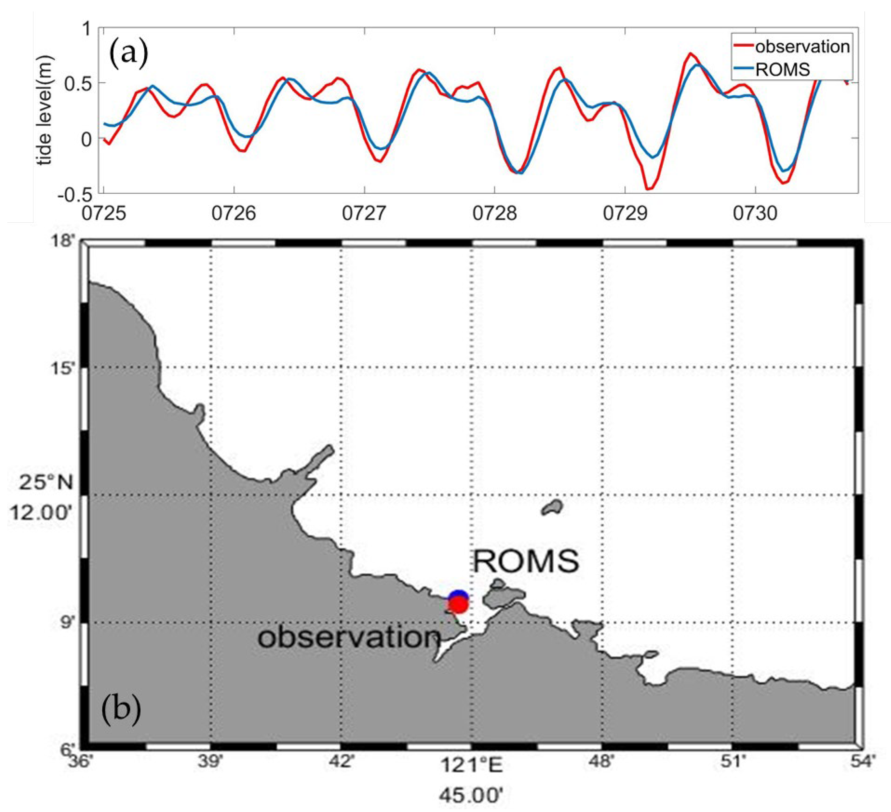
For Wanghaixiang Bay, tidal forcing was considered as the key factor dominating the local oceanic dynamics [24], thus, in our simulations, based on the method described in the study [25], different tidal constituents were integrated into ROMS from its lateral boundaries. Here, tidal constituents including M2, S2, N2, K2, K1, O1 P1, Q1, Mf, and Mm (provided by the Oregon State University global models of ocean tides TPXO7 [26]) were integrated into ROMS. Additionally, the open boundary radiation scheme [27] was applied to ensure the model worked properly. Later on, model-simulated sea-level changes (included tidal forcing) were compared with nearby available tide gauge observations to validate the simulations. Figure 7 shows the comparison of sea-level changes derived from model simulation (blue line) and tide gauge measurements (red line) deployed within Keelung harbor (25.157° N, 121.745° E, http://uhslc.soest.hawaii.edu/data/ (accessed on 22 January 2021)) during July 2008. The root-mean-square error (RMSE) and the correlation coefficient between both sea-level data sources are 0.0792 m and 0.9767, respectively. Although no validation of the model for storm simulation is provided here, numerical simulations were performed based on a ROMS series module with a long heritage, developed mainly for storm simulation. Related validations for the skill of this module can be found in previous studies [27,28,29,30].
4. Results
This study simulated a no-wind scenario, a northeast monsoon scenario, and three typhoon scenarios, considering tidal currents, to understand when the seawall of the coastal landfill is damaged and buried garbage flows into the sea, whether the drift of garbage pollutes the environment of the bay. To understand how the buried garbage drifts after falling into the sea, the model simulated the garbage falling into the sea at three locations close to the landfill site, namely, outer (outside the bay), middle (at the mouth of the bay), and inner (inside the bay), as shown in Figure 1. To predict the path of drifting garbage, the forward-tracking method was used. The formula is as follows:
where t and Δt are the time and time interval of the time step, and are the location of garbage and current at time t, and is the predicated location of the garbage at time t + 1. Since the drifting garbage could be affected by ocean current () and wind (), is considered to be:
where is the coefficient of windage effect, which typically ranges between 0 and 0.05 [31,32,33]. The windage is classified into low windage (0–1%, e.g., fishing nets and small plastic fragments), moderate windage (2–3%, e.g., polystyrene and partially filled PET bottles), or high windage (4–5%, e.g., unfilled PET bottles and fishing buoys) [34]. Due to the variety of garbage in the landfill, the most common is plastic. Therefore, a suggested windage coefficient of 3.5% was used in this study. The probability density is used to represent the movement of the garbage after it falls into the sea. Assuming that garbage falls into the sea at each time step of the numerical model simulation, if garbage drifts past the grid point, it is calculated once, and finally divided by the total time step. In this way, one can figure out where the garbage is most likely to be passed. It should be noted here that if garbage is stranded, it is stranded, and resuspension is not considered.
4.1. No-Wind Scenario
This simulation is dominated by the effects of tidal currents. The simulation time is the period of Typhoon Fung-Wong invading Taiwan, that is, from 0000Z on 20 July to 1750Z on 31 July 2008. Figure 8 shows the probability density of the path of garbage falling into the sea at three locations without wind effects. The high-density area is located where the garbage falls into the sea, and extends northwest–southeast outside the bay. This is consistent with the directions of tidal currents. The tidal current outside the bay flows northwest at flood tide and southeast at ebb tide [24]. That is, the garbage falling into the sea moves with tidal currents. During this period, the average speeds of flood tide and ebb tide were about 0.33 m s−1 and 0.71 m s−1, respectively. The ebb tide is faster than the flood tide. Therefore, the probability density of garbage drifting to the southeast is greater than that to the northwest.
From the distribution of the three subgraphs in Figure 8, it can be seen that if the garbage fell at the inner location (Figure 8a), the probability of the garbage trajectory entering the bay was greater than that falling at the outer location (Figure 8c). Therefore, the probability that the garbage falling at the inner location might get stuck on the shore is higher than that of the garbage falling at the outer location. Although the probability density of each grid point is lower far away from the bay, it means that the garbage would eventually flow out to the ocean, with the ocean currents north of Taiwan flowing into the open ocean.
Figure 9 demonstrates an example of garbage drifting trajectories during ebb and flood tides. Figure 9a shows the simulated water level in northeast Taiwan, and Figure 9b,c demonstrate the drifting trajectories of garbage after falling into the sea at the three locations at the time shown by the red and green dots in Figure 9a, representing the conditions of the ebb tide and the flood tide, respectively. The cases of ebb and flood tides were taken at 0010Z and 0740Z on 28 July, respectively. It can be clearly seen that the garbage drifting trajectory flowed southeast during the ebb tide. Garbage that fell at the inner and the middle locations got stuck on the other side of the mouth of the bay, whereas garbage that fell in the outer location flowed along with the ebb tidal current. During the flood tide, the garbage drifting trajectory was to the northwest and garbage eventually flowed out of the simulation domain.
4.2. Northeast Monsoon Scenario
This simulation considers the drifting trajectory of garbage under the strong northeast monsoon and tidal currents. The simulation period is the same as that of the no-wind scenario. Figure 10 presents the simulation results of the probability density of the drifting trajectories of garbage falling into the sea at three locations under the prevailing 10 m s−1 northeast monsoon. The distribution of the probability density is quite different from the no-wind scenario. The drifting garbage caused by the prevailing northeast monsoon was largely stranded on the shore. Most of the garbage falling at the inner location was stranded on the shore inside the bay, while falling at the middle location was stranded on the shore inside and outside the bay. If the garbage falls at the outer location, it has the opportunity to flow across the bay, but still mostly stranded on the shore near the place where the garbage fell into the sea. Since the windage is set to 3.5% in this study, a northeasterly wind speed of 10 m s−1 may result in a southward flow of 0.25 m s−1 and a westward flow of 0.25 m s−1. Although the wind-induced garbage drifts at a drifting speed smaller than that of the mean tidal current, it is assumed here that the northeast monsoon is blowing continuously. Nevertheless, it is worth noting that this might not be a truly physical scenario. As a result, the garbage is eventually confined to the shore by the wind. The drifting trajectories of garbage falling at the outer location are somewhat different from those falling at the inner and middle locations. The possible reason is that the outer location is more affected by tidal currents, so the drifting trajectories can flow through most of the bay.
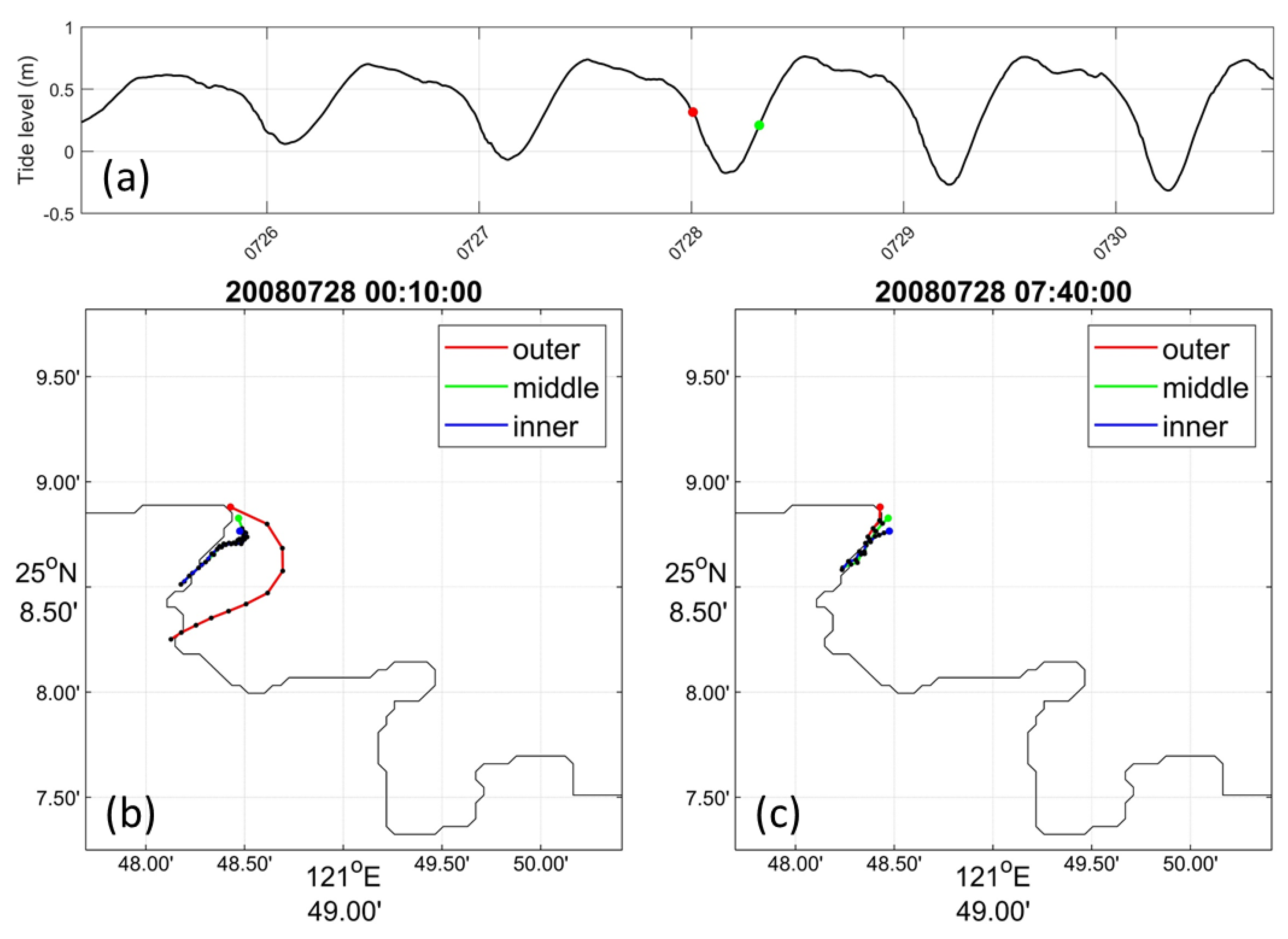
An example of garbage trajectories during ebb and flood tides in the northeast monsoon period is shown in Figure 11. Figure 11a shows the simulated water level in northeast Taiwan. Figure 11b,c demonstrate the drifting trajectories of the garbage falling into the sea at the three locations at the time indicated by the red and green dots, respectively, in Figure 11a. The time of simulation is the same as that in Figure 9a. Due to the influence of the northeast monsoon, during the ebb tide, the garbage falling at the inner and the middle locations was soon blown to the coast. The garbage that fell in the outer location was initially affected by tidal currents and drifted to the southeast, but was finally blown into the bay by the northeast monsoon. During the flood tide period, no matter where the garbage fell, it soon drifted into the bay and was stranded on the shore.
4.3. Typhoon Scenarios
Three typhoon scenarios were simulated using ROMS to consider the effects of tidal currents and typhoons. These typhoons are randomly selected. One passed through central Taiwan, Typhoon Fung-Wong (2008), another passed through northern Taiwan, Typhoon Soulik (2013), and the other passed through outside northern Taiwan, Typhoon Sinlaku (2002).
4.3.1. Typhoon Fung-Wong (2008)
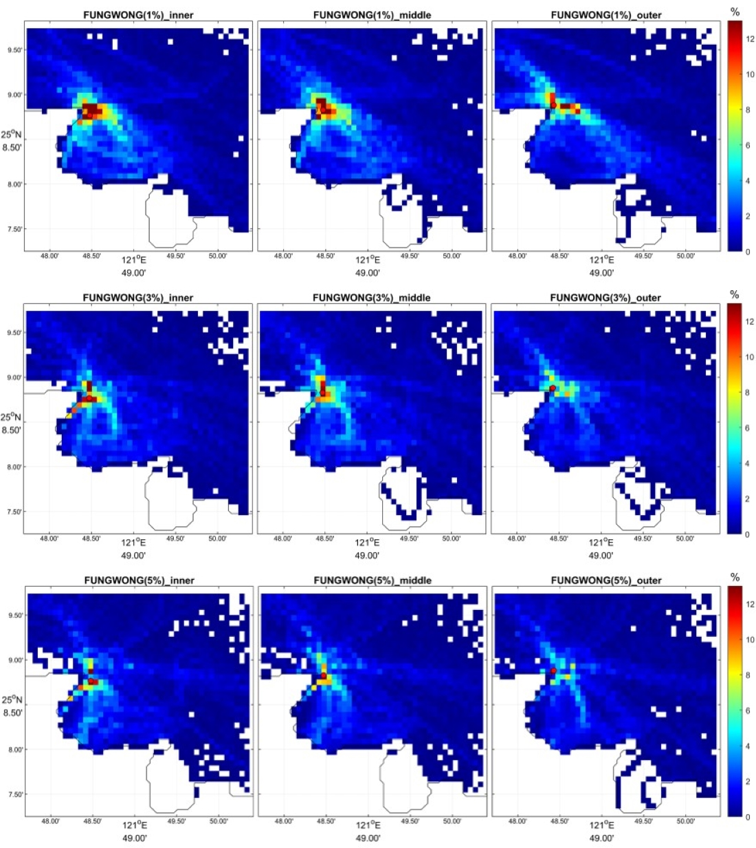
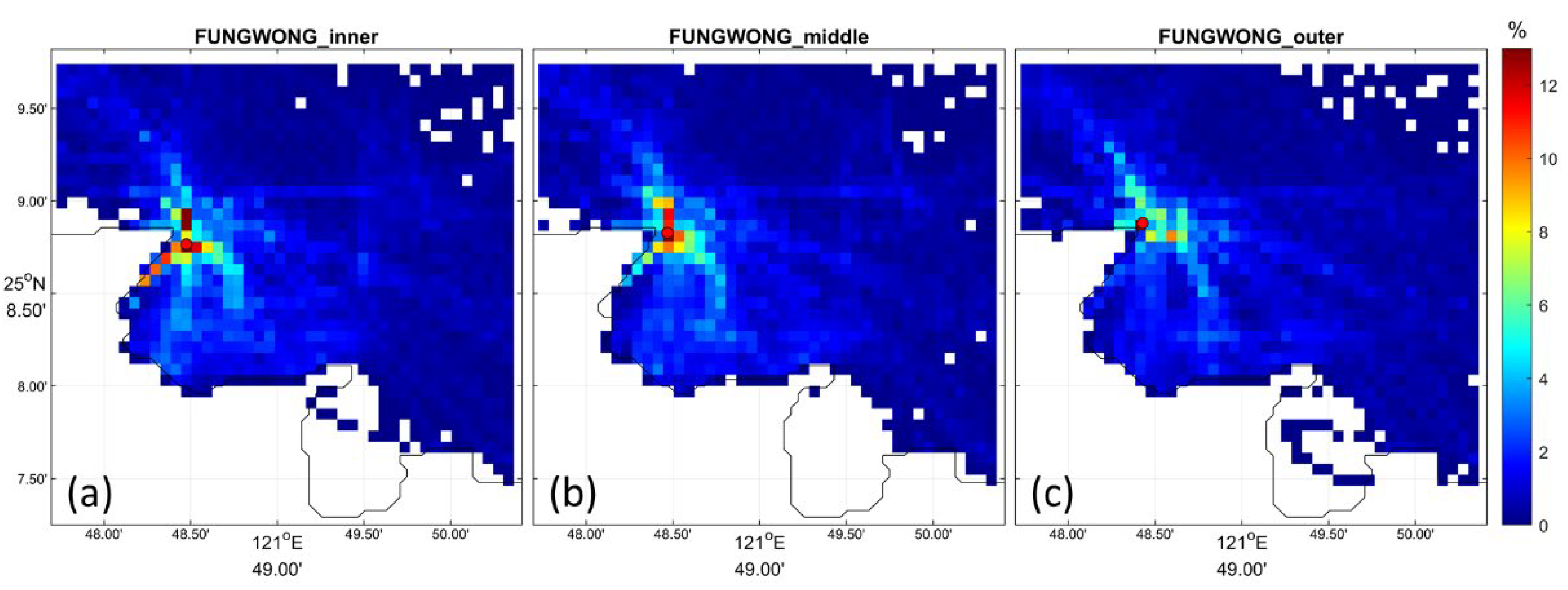
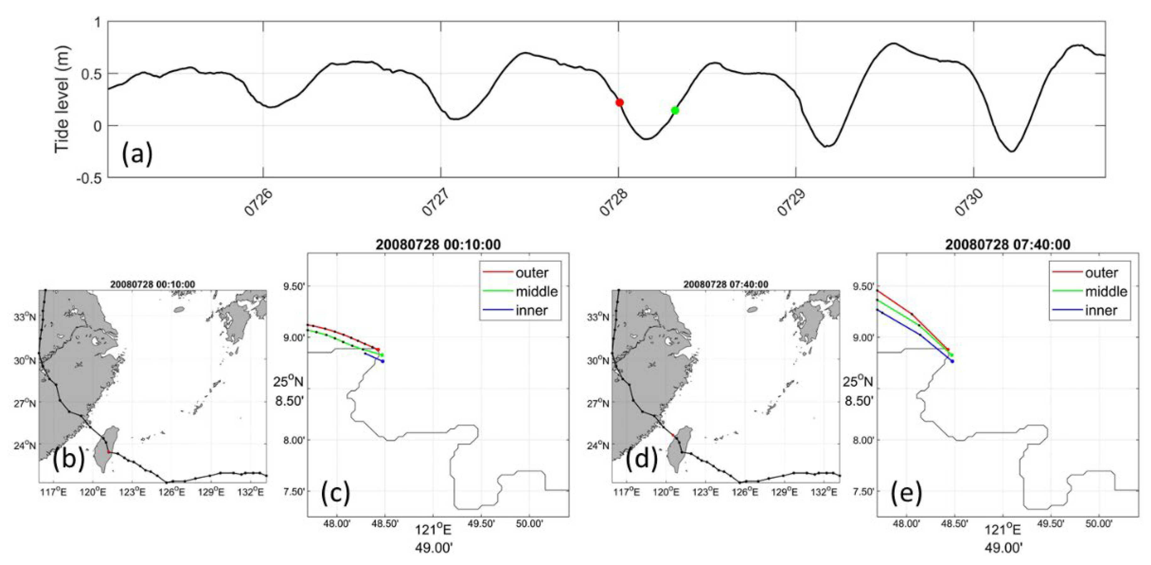
The effect of Typhoon Fung-Wong (2008) and the tidal current is considered in this simulation case. Typhoon Fung-Wong (2008), a Category 2 typhoon on the Saffir-Simpson Hurricane Scale, hit Taiwan with high winds, rain, and storm surge on 28 July 2008. Its center crossed Taiwan almost along Route 2, as shown in Figure 5. The typhoon formed at 0600Z on 25 July and became a tropical depression at 1200Z on 29 July. It landed in Taiwan at 0000Z on 28 July and entered the Taiwan Strait at 0630Z on 28 July. Figure 12 shows the probability density of the garbage drift trajectory from 0300Z on 25 July to 1750Z on 30 July, including the period of the typhoon landing on Taiwan. The wind data were taken from the ECMWF data set. From the probability density of the trajectory, it is more diverse due to the influence of the typhoon. It is often higher on the coast near the landfill. When the garbage fell at the inner and the middle locations, it would have a higher chance of stranded on the coast of the bay. As the typhoon continued to move and the wind direction changed constantly, the trajectories of garbage drifting caused by the typhoon are widely distributed. Additionally, the underlying high-wind condition was accompanied with certain typhoon passage, showing that the tidal effect no longer dominates the landfill dynamic surrounding the bay.
Figure 13 shows an example of garbage drift trajectories during ebb and flood tides. The times of ebb and flood tides for demostration are the same as those in Figure 9 and Figure 11. The time of ebb tide was when the typhoon had just landed on eastern Taiwan. The drifting garbage did not drift to the southeast with the tidal current. Instead, it was affected by the typhoon and drifted to the northwest. The time of flood tide was when the typhoon left the land of Taiwan. Probably unaffected by the typhoon, the drifting garbage flowed northwestward, that is, along the direction of the flood tidal current. This means that tidal currents were more dominant at this time.
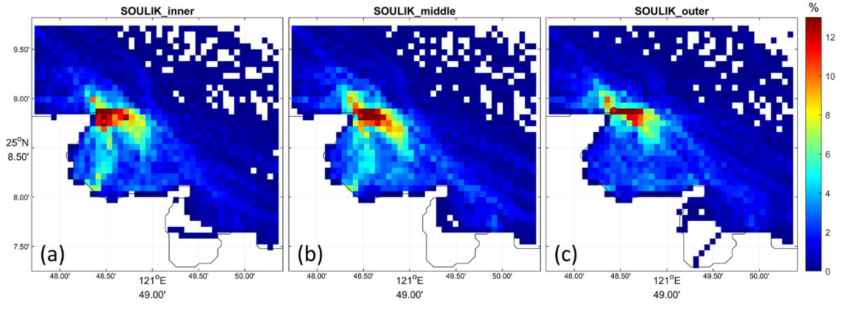
4.3.2. Typhoon Soulik (2013)
Typhoon Soulik (2013) formed on 7 July 2013 and dissipated on 14 July 2013. The Central Weather Bureau of Taiwan issued a warning at 1230Z on 11 July, and the warning was lifted at 1530Z on 13 July. The typhoon landed on Taiwan at 0700Z on 12 July and left at 1600Z on 12 July. Its center crossed Taiwan, almost along Route 2 (see Figure 5). Figure 14 shows the probability density of the garbage drift trajectory from the three garbage falling locations between 0600Z on 9 July 2013 and 1750Z on 13 July 2013. The wind data used in this simulation were also taken from the ECMWF data set. The typhoon forced most of the garbage into the bay, especially the garbage that fell into sea from the inner and the middle locations. This can be found from the probability density of the trajectory of garbage. A higher probability trajectory was seen within the bay. However, a higher probability trajectory was also clearly seen in the northwest–southeast direction outside the bay, which means that tidal currents still affected the drift of garbage even during the typhoon period. Compared with the case of Typhoon Fung-Wong (2008), Typhoon Soulik (2013) had a higher probability of garbage entering the bay, probably because the Typhoon Soulik (2013) track was closer to the landfill.
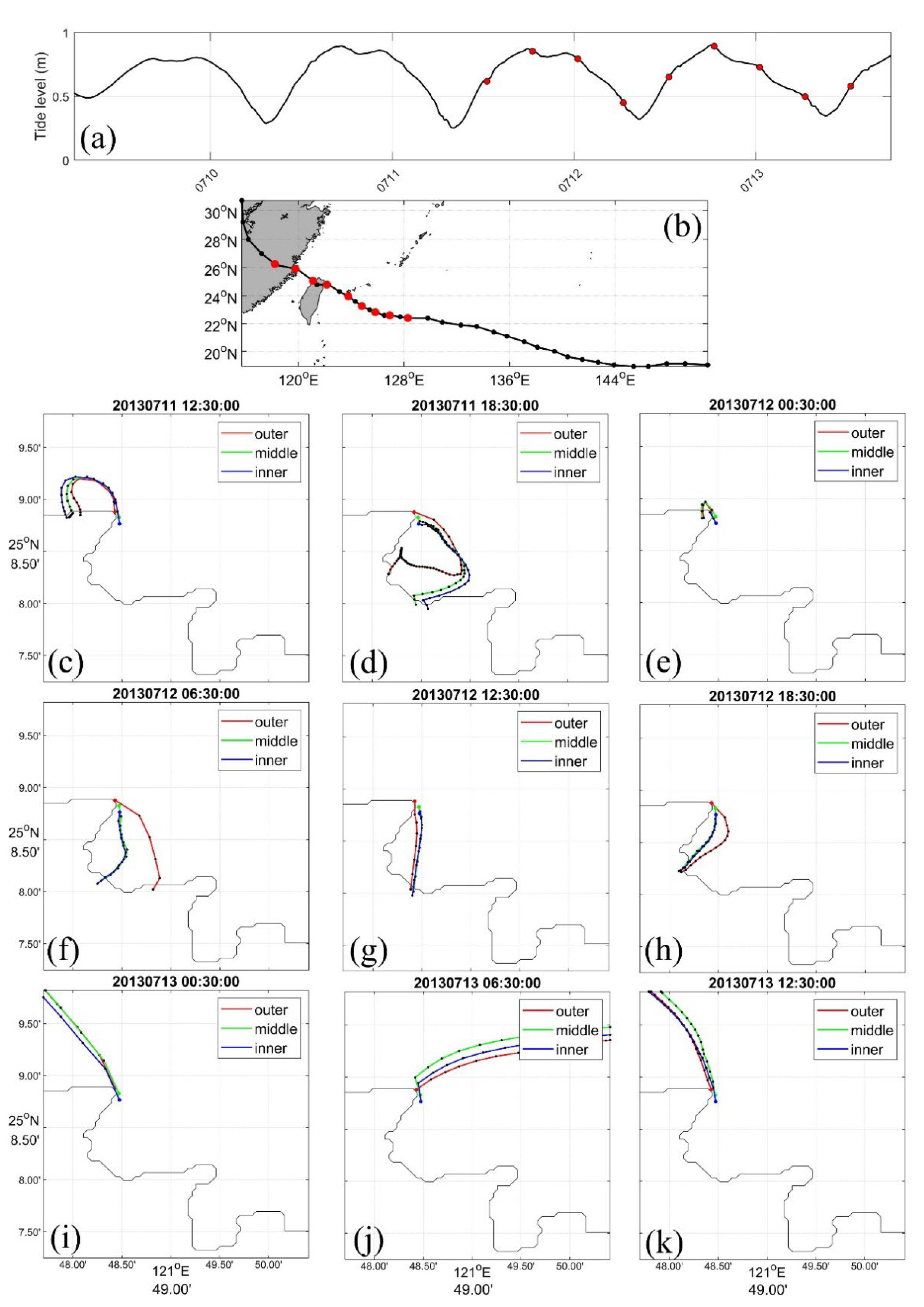
To understand the influence of typhoon Soulik (2013) on garbage drifting, Figure 15 shows the garbage drifting trajectories during the period of the influence of typhoon on Taiwan. The time is from 1230Z on 11 July to 1230Z on 13 July, every six hours for the simulation of garbage drifting. The simulated time period is roughly the same as when the typhoon warning was issued and lifted. Figure 15a shows the tidal level. The red dots on the figure from left to right correspond to the time of Figure 15c–k. Figure 15b is the typhoon track, and the red dots on the figure from left to right indicate the time corresponding to Figure 15c–k.
Figure 15c shows the garbage drift trajectory at flood tide. The garbage first drifted to the northeast, and then was affected by the typhoon and drifted toward the coast. After that, the garbage drifting was affected by the typhoon. As the typhoon got closer to Taiwan, regardless of flood tide, ebb tide or slack tide, the garbage basically drifted into the bay. At 0030Z on 13 July (Figure 15i), the typhoon was about to leave Taiwan, and its position relative to the study area was also different from the previous ones. The change of wind direction caused the garbage to drift northwest. After the typhoon was far away, the direction of the garbage drift was again affected by tidal currents. It went southeast at ebb tide and northwest at flood tide.
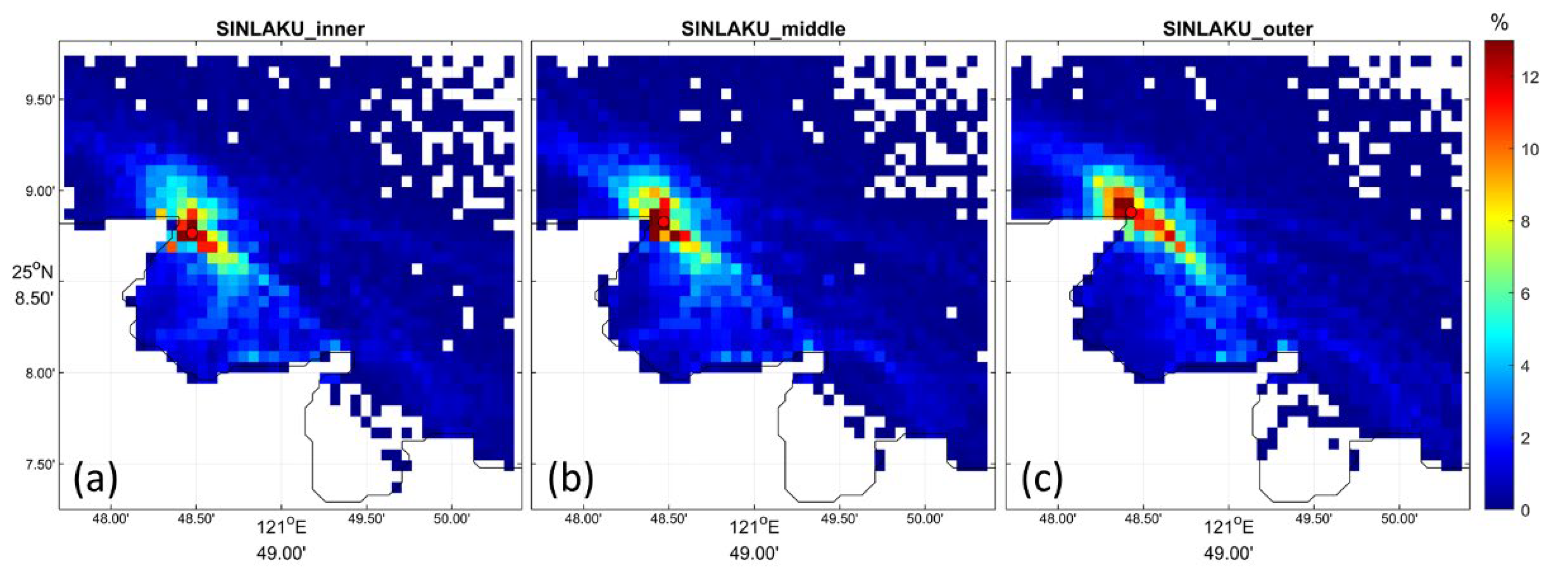
4.3.3. Sinlaku (2002)
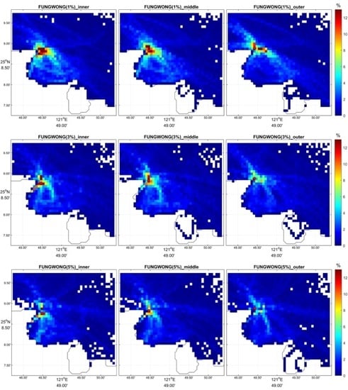
Typhoon Sinlaku (2002), which is a Category 3 typhoon, was formed on 27 August 2002 and dissipated on 8 September 2002. The Central Weather Bureau of Taiwan issued a warning at 2115Z on 4 September and lifted the warning at 2150Z on 7 September. The typhoon passed through the sea off northern Taiwan. Its path is classified as Route 1 (see Figure 5). Figure 16 shows the probability density of the simulated garbage drift trajectories for the three garbage falling locations from 0600Z on 2 September 2002 to 1750Z on 8 September 2002. Wind data were also taken from the ECMWF data set. The probability density distribution of this case entering the bay is less than that of Typhoon Soulik (2013). This may be because the typhoon paths are different, and the wind direction in the study area is also different. The highest probability densities were on the coast near the landfill, and higher probability densities were along the northwest–southeast direction, which seems to be in the direction of tidal current, especially for garbage falling at the outer location.
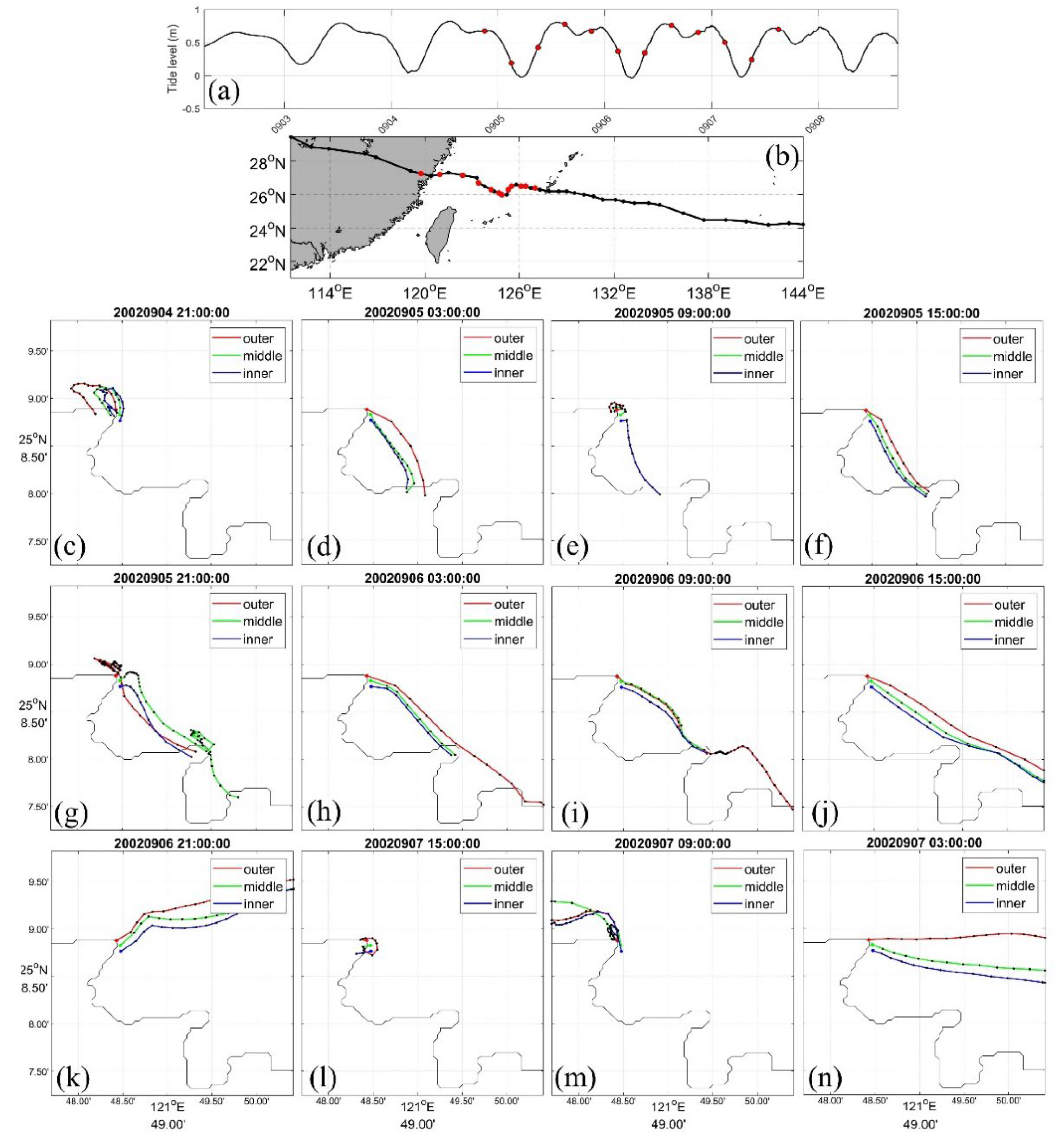
The same as Figure 15, Figure 17 shows the garbage trajectories at three locations from 2100Z on 4 September when the Typhoon Sinlaku (2002) warning was issued to 0900Z on 7 September when the typhoon warning was nearly lifted. It is clear that these trajectories were not driven by tidal currents, but forced by the typhoon. Whether at ebb tide, flood tide, or slack tide, garbage was almost always drifting to shore. After the typhoon warning was lifted, the garbage began to drift in the directions of tide currents.
5. Discussion
From the numerical simulation of the garbage falling into the sea near Wanghaixiang Bay near the landfill site, it can be seen that under the influence of no-wind, the trajectories of the garbage falling into the sea were basically affected by tidal currents. During the northeast monsoon, because the wind blew to the shore, the garbage basically flowed to the shore due to the windage effect. However, the location where the garbage fell into the sea may affect the situation of the garbage drifting. The garbage that fell in the bay or at the mouth of the bay would drift to the shore, but it would soon be stranded on the shore. Affected by the windage effect and tidal currents, the garbage that fell outside the bay would drift in most of the bay before finally stranded on the shore. Since the variety of garbage in the landfill, a moderate windage coefficient of 3.5% was selected for simulation in this study. The actual drifting situation may vary depending on the type of garbage that falls into the sea.
High waves caused by typhoons can damage the protection of the landfill, allowing for garbage to fall into the sea. From the simulations of the three typhoon tracks that may have an impact on the northern waters of Taiwan, it can be seen that the effects are somehow different. Although the track of typhoon is different in distance and direction from the study area, the strong wind speed of the typhoon has the same effect on the falling garbage. Affected by the wind, the garbage that fell into the sea basically flowed to the shore. However, as the typhoon continued to advance, the wind direction kept changing. Unlike the northeast monsoon scenario, the wind continues to blow in the same direction, so the trajectories of garbage drifting were somewhat different.
In this study, the trajectory analysis was performed based on the current field output from the model simulation. It is worth noting that there is definitely a discrepancy between the simulated garbage drift and the actual garbage movement due to the slightly different properties of the simulated surface trajectory and the actual garbage.
6. Conclusions
The landfill site in Wanghaixiang Bay has experienced many typhoons and strong northeast monsoons. The protective embankment of the landfill site is sometimes damaged. The buried garbage is exposed and knocked down by waves and becomes marine garbage. To understand the impact of this falling sea garbage on the environment, this study used a numerical model to simulate drifting conditions during periods of no-wind, northeast monsoons, and typhoons. From the simulation results, the flow field in Wanghaixiang Bay is shown to mainly be affected by tides in the no-wind scenario. In the northeast monsoon scenario, the windage factor forces the garbage to flow to the coast. During the typhoon period, strong winds force garbage to the coast or to the open ocean, depending on the path and wind direction of the typhoon.
Author Contributions
Conceptualization, C.-R.H. and L.-C.C.; methodology, Y.-H.L.; software, C.-Y.L. and Z.-W.Z.; validation, Z.-W.Z.; formal analysis, Y.-H.L. and C.-R.H.; investigation, Y.-H.L.; resources, C.-R.H.; data curation, C.-Y.L.; writing—original draft preparation, Y.-H.L., Z.-W.Z. and C.-R.H.; writing—review and editing, C.-R.H. and L.-C.C.; visualization, C.-Y.L.; supervision, C.-R.H.; funding acquisition, C.-R.H. All authors have read and agreed to the published version of the manuscript.
Funding
This research was funded by Ministry of Science and Technology of Taiwan, grant number MOST110-2611-M-019-001.
Data Availability Statement
All data sets used in this study can be publicly archived. Wind data can be found through the website of Central Weather Bureau of Taiwan at https://www.cwb.gov.tw/V8/C/W/OBS_Station.html (accessed on 22 January 2021). Tide gauge data can be archived at http://uhslc.soest.hawaii.edu/data/ (accessed on 22 January 2021).
Acknowledgments
The authors thanks to Yi-Chung Yang for preparing some figures. Thanks also to CWB, ROMS, and HYCOM science team for providing the essential data sets. Two anonymous reviewers provided valuable comments that helped improve this paper.
Conflicts of Interest
The authors declare no conflict of interest.
References
- Van Sebille, E.; Aliani, S.; Law, K.L.; Maximenko, N.; Alsina, J.M.; Bagaev, A.; Bergmann, M.; Chapron, B.; Chubarenko, I.; Cózar, A.; et al. The physical oceanography of the transport of floating marine debris. Environ. Res. Lett. 2020, 15, 023003. [Google Scholar] [CrossRef] [Green Version]
- Martinez, E.; Maamaatuaiahutapu, K.; Taillandier, V. Floating marine debris surface drift: Convergence and accumulation toward the South Pacific subtropical gyre. Mar. Pollut. Bull. 2009, 58, 1347–1355. [Google Scholar] [CrossRef]
- Martínez-Vicente, V.; Clark, J.R.; Corradi, P.; Aliani, S.; Arias, M.; Bochow, M.; Bonnery, G.; Cole, M.; Cózar, A.; Donnelly, R.; et al. Measuring marine plastic debris from space: Initial assessment of observation requirements. Remote Sens. 2019, 11, 2443. [Google Scholar] [CrossRef] [Green Version]
- Kikaki, A.; Karantzalos, K.; Power, C.A.; Raitsos, D.E. Remotely Sensing the Source and Transport of Marine Plastic Debris in Bay Islands of Honduras (Caribbean Sea). Remote Sens. 2020, 12, 1727. [Google Scholar] [CrossRef]
- Merlino, S.; Paterni, M.; Berton, A.; Massetti, L. Unmanned aerial vehicles for debris survey in coastal areas: Long-term monitoring programme to study spatial and temporal accumulation of the dynamics of beached marine litter. Remote Sens. 2020, 12, 1260. [Google Scholar] [CrossRef] [Green Version]
- Hardesty, B.D.; Harari, J.; Isobe, A.; Lebreton, L.; Maximenko, N.; Potemra, J.; van Sebille, E.; Vethaak, A.D.; Wilcox, C. Using numerical model simulations to improve the understanding of micro-plastic distribution and pathways in the marine environment. Front. Mar. Sci. 2017, 4, 30. [Google Scholar] [CrossRef] [Green Version]
- Lebreton, L.C.M.; Greer, S.D.; Borrero, J.C. Numerical modelling of floating debris in the world’s oceans. Mar. Pollut. Bull. 2012, 64, 653–661. [Google Scholar] [CrossRef]
- Potemra, J.T. Numerical modeling with application to tracking marine debris. Mar. Pollut. Bull. 2012, 65, 42–50. [Google Scholar] [CrossRef]
- Maes, C.; Blanke, B. Tracking the origins of plastic debris across the Coral Sea: A case study from the Ouvéa Island, New Caledonia. Mar. Pollut. Bull. 2015, 97, 160–168. [Google Scholar] [CrossRef]
- Pereiro, D.; Souto, C.; Gago, J. Calibration of a marine floating litter transport model. J. Oper. Oceanogr. 2018, 11, 125–133. [Google Scholar] [CrossRef]
- Maximenko, N.; Corradi, P.; Law, K.L.; Van Sebille, E.; Garaba, S.P.; Lampitt, R.S.; Galgani, F.; Martinez-Vincete, V.; Goddijn-Murphy, L.; Veiga, J.M.; et al. Towards the integrated marine debris observing system. Front. Mar. Sci. 2019, 6, 447. [Google Scholar] [CrossRef] [Green Version]
- Veiga, J.M.; Fleet, D.; Kinsey, S.; Nilsson, P.; Vlachogianni, T.; Werner, S.; Galgani, F.; Thompson, R.C.; Dagevos, J.; Gago, J.; et al. Identifying sources of marine litter. MSFD GES TG Marine Litter Thematic Report. In JRC Technical Report 2016; European Commission: Brussels, Belgium, 2016; 43p. [Google Scholar]
- Beaven, R.P.; Stringfellow, A.M.; Nicholls, R.J.; Haigh, I.D.; Kebede, A.S.; Watts, J. The impact of coastal landfills on shoreline management plans. In Sardinia 2017: 16th International Waste Management and Landfill Symposium; CISA Publisher: Padova, Italy, 2007; pp. 1–12. [Google Scholar]
- Beaven, R.P.; Stringfellow, A.M.; Nicholls, R.J.; Haigh, I.D.; Kebede, A.S.; Watts, J. Future challenges of coastal landfills exacerbated by sea level rise. Waste Manag. 2020, 105, 92–101. [Google Scholar] [CrossRef] [PubMed]
- Brand, J.H. Assessing the Risk of Pollution from Historic Coastal Landfills. Ph.D. Thesis, Queen Mary University of London, London, UK, 2017. [Google Scholar]
- Parker, B.B. Tidal Analysis and Prediction; NOAA Special Publication NOS CO-OPS 3; U.S. Department of Commerce: Washington, DC, USA, 2007; 378p.
- Pereiro, D.; Souto, C.; Gago, J. Dynamics of floating marine debris in the northern Iberian waters: A model approach. J. Sea Res. 2019, 144, 57–66. [Google Scholar] [CrossRef]
- Zaleski, S.F.; Watabayashi, G.; Dong, C.; Barker, C.H.; MacFadyen, A.; Righi, D.; Kachook, G.; Zelenke, B. Predicting surface oil transport in California using a high-resolution Regional Ocean Modeling System (ROMS) and the National Oceanic and Atmospheric Administration’s (NOAA’s) Trajectory Analysis Planner (TAP). Int. Oil Spill Conf. Proc. 2017, 2017, 2017309. [Google Scholar] [CrossRef]
- Carlson, D.F.; Suaria, G.; Aliani, S.; Fredj, E.; Fortibuoni, T.; Griffa, A.; Russo, A.; Melli, V. Combining Litter Observations with a Regional Ocean Model to Identify Sources and Sinks of Floating Debris in a Semi-enclosed Basin: The Adriatic Sea. Front. Mar. Sci. 2017, 4, 78. [Google Scholar] [CrossRef] [Green Version]
- Shchepetkin, A.F.; McWilliams, J.C. A method for computing horizontal pressure-gradient force in an oceanic model with a non-aligned vertical coordinate. J. Geophys. Res. 2003, 108, 3090. [Google Scholar] [CrossRef]
- Shchepetkin, A.F.; McWilliams, J.C. The Regional Ocean Modeling System (ROMS): A split-explicit, free-surface, topography-following coordinates ocean model. Ocean Model. 2005, 9, 347–404. [Google Scholar] [CrossRef]
- Moore, A.M.; Arango, H.G.; Miller, A.J.; Cornuelle, B.D.; Di Lorenzo, E.; Neilson, D.J. A comprehensive ocean prediction and analysis system based on the tangent linear and adjoint of a regional ocean model. Ocean Model. 2004, 7, 227–258. [Google Scholar] [CrossRef]
- Warner, J.C.; Geyer, W.R.; Lerczak, J.A. Numerical modeling of an estuary: A comprehensive skill assessment. J. Geophys. Res. 2005, 110, C05001. [Google Scholar] [CrossRef]
- Chen, K.Y.; Huang, C.F.; Huang, S.W.; Liu, J.Y.; Guo, J. Mapping coastal circulations using moving vehicle acoustic tomography. J. Acoust. Soc. Am. 2020, 148, EL353–EL358. [Google Scholar] [CrossRef]
- Flather, R.A. A tidal model of the northwest European continental shelf. Mem. Soc. Roy. Sci. Liege 1976, 10, 141–164. [Google Scholar]
- Egbert, G.; Erofeeva, S. Efficient inverse modeling of barotropic ocean tides. J. Atmos. Ocean. Technol. 2020, 19, 183–204. [Google Scholar] [CrossRef] [Green Version]
- Zheng, Z.W.; Zheng, Q.; Lee, C.Y.; Gopalakrishnan, G. Transient modulation of Kuroshio upper layer flow by directly impinging typhoon Morakot in east of Taiwan in 2009. J. Geophys. Res. Oceans 2014, 119, 4462–4473. [Google Scholar] [CrossRef]
- Zheng, Z.W.; Zheng, Q.; Gopalakrishnan, G.; Kuo, Y.C.; Yeh, T.K. Response of upper ocean cooling off northeastern Taiwan to typhoon passages. Ocean Model. 2017, 115, 105–118. [Google Scholar] [CrossRef]
- Zheng, Z.W.; Ho, C.R.; Zheng, Q.; Lo, Y.T.; Kuo, N.J.; Gopalakrishnan, G. Effects of preexisting cyclonic eddies on upper ocean responses to Category 5 typhoons in the western North Pacific. J. Geophys. Res. Oceans 2010, 115, C09013. [Google Scholar] [CrossRef]
- Shen, D.; Li, X.; Wang, J.; Bao, S.; Pietrafesa, L.J. Dynamical ocean responses to Typhoon Malakas in the vicinity of Taiwan. J. Geophys. Res. Oceans 2021, 126, e2020JC016663. [Google Scholar] [CrossRef]
- Duhec, A.V.; Jeanne, R.F.; Maximenko, N.; Hafner, J. Composition and potential origin of marine debris stranded in the Western Indian Ocean on remote Alphonse Island, Seychelles. Mar. Pollut. Bull. 2015, 96, 76–86. [Google Scholar] [CrossRef]
- Allshouse, M.R.; Ivey, G.N.; Lowe, R.J.; Jones, N.L.; Beegle-Krause, C.J.; Xu, J.; Peacock, T. Impact of windage on ocean surface Lagrangian coherent structures. Environ. Fluid Mech. 2017, 17, 473–483. [Google Scholar] [CrossRef]
- Ko, C.T.; Hsin, Y.C.; Jeng, M.S. Global distribution and cleanup opportunities for macro ocean litter: A quarter century of accumulation dynamics under windage effects. Environ. Res. Lett. 2020, 15, 104063. [Google Scholar] [CrossRef]
- Onink, V.; Wichmann, D.; Delandmeter, P.; van Sebille, E. The role of Ekman current, geostrophy, and Stokes drift in the accumulation of floating microplastic. J. Geophys. Res. Oceans 2019, 124, 1474–1490. [Google Scholar] [CrossRef] [Green Version]
Figure 1.
The study area. The three red dots are the landfill garbage falling positions in the numerical model simulations (image source: Google Earth).
Figure 1.
The study area. The three red dots are the landfill garbage falling positions in the numerical model simulations (image source: Google Earth).

Figure 2.
The exposed garbage of the landfill in Keelung caused by wind waves in 2011 (photo provided by the National Museum of Marine Science and Technology).
Figure 2.
The exposed garbage of the landfill in Keelung caused by wind waves in 2011 (photo provided by the National Museum of Marine Science and Technology).

Figure 3.
Six major tidal constituents in Keelung, Taiwan.

Figure 4.
Wind and wind gust roses in Keelung, Taiwan from 2011 to 2020.

Figure 5.
(a) Statistics of nine typhoon routes to hit Taiwan from 1897 to 2014, data adapted from http://www.tyroom.url.tw/pages/body_09.htm (accessed on 22 January 2021); (b–d) typhoon tracks of Sinlaku (2002), Soulik (2013), and Fung-Wong (2008), respectively (adapted from Wikipedia) (image source: © Google, Imagery ©2020 TerraMetics, Google Earth).

Figure 6.
(a) The 5-layers nesting model domains (parent and children); (b) Lateral boundary conditions (temperature) derived from HYCOM/NCODA and used in the model simulations.
Figure 6.
(a) The 5-layers nesting model domains (parent and children); (b) Lateral boundary conditions (temperature) derived from HYCOM/NCODA and used in the model simulations.

Figure 7.
(a) Model-simulated sea-level changes derived from model simulation (blue line) and tide gauge measurements (red line) deployed within Keelung harbor (nearest site, 25.157° N, 121.745° E) during July 2008; (b) Locations of Keelung Harbor tide gauge (red dot) and corresponding nearest available model grid (blue dot).

Figure 8.
The probability density of the path of garbage falling into the sea at three locations without wind effects: (a) inner; (b) middle; (c) outer during the simulation data time span. The number in the color bar represents the percentage of garbage passing.
Figure 8.
The probability density of the path of garbage falling into the sea at three locations without wind effects: (a) inner; (b) middle; (c) outer during the simulation data time span. The number in the color bar represents the percentage of garbage passing.

Figure 9.
(a) The simulated water level at northeast Taiwan; (b) garbage trajectory at the time of the red point on (a) falling into the sea; (c) the same as (b) but at the time of the green point. The blue, green, and red lines on (b,c) represent the trajectories of garbage falling at inner, middle, and outer locations, respectively.

Figure 10.
Same as Figure 8, but for the northeast monsoon scenario; (a) inner; (b) middle; (c) outer during the simulation data time span. The number in the color bar represents the percentage of garbage passing.
Figure 10.
Same as Figure 8, but for the northeast monsoon scenario; (a) inner; (b) middle; (c) outer during the simulation data time span. The number in the color bar represents the percentage of garbage passing.

Figure 11.
Same as Figure 9, but for the northeast monsoon scenario. (a) The simulated water level at northeast Taiwan; (b) garbage trajectory at the time of the red point on (a) falling into the sea; (c) the same as (b) but at the time of the green point. The blue, green, and red lines on (b,c) represent the trajectories of garbage falling at inner, middle, and outer locations, respectively.

Figure 12.
Same as Figure 8, but for the Typhoon Fung-Wong (2008) case; (a) inner; (b) middle; (c) outer during the simulation data time span. The number in the color bar represents the percentage of garbage passing.
Figure 12.
Same as Figure 8, but for the Typhoon Fung-Wong (2008) case; (a) inner; (b) middle; (c) outer during the simulation data time span. The number in the color bar represents the percentage of garbage passing.

Figure 13.
Typhoon Fung-Wong (2008) case. (a) The simulated water level at northeast Taiwan; (b) Typhoon Fung-Wong (2008) track. The red dot represents the time of typhoon location at the time of red point on (a); (c) Garbage trajectory at the time of the red point on (a) falling into the sea; (d) The same as (b) but at the time of the green point on (a); (e) The same as (c) but at the time of the green point on (a). The blue, green, and red lines on (c,e) represent the trajectories of garbage falling at inner, middle, and outer locations, respectively.

Figure 14.
Same as Figure 8, but for the Typhoon Soulik (2013) case; (a) inner; (b) middle; (c) outer during the simulation data time span. The number in the color bar represents the percentage of garbage passing.
Figure 14.
Same as Figure 8, but for the Typhoon Soulik (2013) case; (a) inner; (b) middle; (c) outer during the simulation data time span. The number in the color bar represents the percentage of garbage passing.

Figure 15.
The drifting trajectory of garbage during the warning period Typhoon Soulik (2013). (a) The simulated water level at northeast Taiwan; (b) Typhoon Soulik (2013) track; (c–k) The drifting trajectory of the garbage after it fell into the sea at the time indicated at the top of the figure. The red dots from left to right in (a) and from right to left in (b) corresponds to the time in (c–k).

Figure 16.
Same as Figure 8, but for the Typhoon Sinlaku (2002) case; (a) inner; (b) middle; (c) outer during the simulation data time span. The number in the color bar represents the percentage of garbage passing.
Figure 16.
Same as Figure 8, but for the Typhoon Sinlaku (2002) case; (a) inner; (b) middle; (c) outer during the simulation data time span. The number in the color bar represents the percentage of garbage passing.

Figure 17.
The drifting trajectory of garbage during the warning period Typhoon Sinlaku (2002). (a) The simulated water level at northeast Taiwan; (b) Typhoon Sinlaku (2002) track; (c–n) The drifting trajectory of the garbage after it fell into the sea at the time indicated at the top of the figure. The red dots from left to right in (a) and from right to left in (b) corresponds to the time in (c–n).


Table 1.
Information of typhoon used in this study (from Typhoon Database https://rdc28.cwb.gov.tw/TDB/public/warning_typhoon_list/ (accessed on 22 January 2021).
Table 1.
Information of typhoon used in this study (from Typhoon Database https://rdc28.cwb.gov.tw/TDB/public/warning_typhoon_list/ (accessed on 22 January 2021).
| Typhoon Name | Warning Period | Lowest Pressure | Highest Wind Speed | Route |
|---|---|---|---|---|
| Fung-Wong (2008) | 0330Z 26 July–0330Z 29 July | 948 hPa | 43 m/s | 3 |
| Soulik (2013) | 0030Z 07 July–1530Z 13 July | 925 hPa | 51 m/s | 2 |
| Sinlaku (2002) | 2115Z 03 September–2150Z 07 September | 950 hPa | 40 m/s | 1 |
Publisher’s Note: MDPI stays neutral with regard to jurisdictional claims in published maps and institutional affiliations. |
© 2022 by the authors. Licensee MDPI, Basel, Switzerland. This article is an open access article distributed under the terms and conditions of the Creative Commons Attribution (CC BY) license (https://creativecommons.org/licenses/by/4.0/).
Share and Cite
MDPI and ACS Style
Lai, Y.-H.; Lu, C.-Y.; Zheng, Z.-W.; Chiang, L.-C.; Ho, C.-R. Numerical Simulation of the Trajectory of Garbage Falling into the Sea at the Coastal Landfill in Northeast Taiwan. Water 2022, 14, 1251. https://doi.org/10.3390/w14081251
AMA Style
Lai Y-H, Lu C-Y, Zheng Z-W, Chiang L-C, Ho C-R. Numerical Simulation of the Trajectory of Garbage Falling into the Sea at the Coastal Landfill in Northeast Taiwan. Water. 2022; 14(8):1251. https://doi.org/10.3390/w14081251
Chicago/Turabian StyleLai, Yu-Hsuan, Ching-Yuan Lu, Zhe-Wen Zheng, Li-Chun Chiang, and Chung-Ru Ho. 2022. "Numerical Simulation of the Trajectory of Garbage Falling into the Sea at the Coastal Landfill in Northeast Taiwan" Water 14, no. 8: 1251. https://doi.org/10.3390/w14081251
Note that from the first issue of 2016, this journal uses article numbers instead of page numbers. See further details here.