A Framework for Comparing Multi-Objective Optimization Approaches for a Stormwater Drainage Pumping System to Reduce Energy Consumption and Maintenance Costs

Abstract

Reducing energy consumption and maintenance costs of a pumping system is seen as an important but difficult multi-objective optimization problem. Many evolutionary algorithms, such as particle swarm optimization (PSO), multi-objective particle swarm optimization (MOPSO), and non-dominated sorting genetic algorithm II (NSGA-II) have been used. However, a lack of comparison between these approaches poses a challenge to the selection of optimization approach for stormwater drainage pumping stations. In this paper, a new framework for comparing multi-objective approaches is proposed. Two kinds of evolutionary approaches, single-objective optimization and multi-objective optimization, are considered. Three approaches representing these two types are selected for comparison, including PSO with linear weighted sum method (PSO-LWSM), MOPSO with technique for order preference by similarity to an ideal solution (MOPSO-TOPSIS), and NSGA-II with TOPSIS (NSGA-II-TOPSIS). Four optimization objectives based on the number of pump startups/shutoffs, working hours, energy consumption, and drainage capacity are considered, of which the first two are new ones quantified in terms of operational economy in this paper. Two comparison methods—TOPSIS and operational economy and drainage capacity (E&C)—are used. The framework is demonstrated and tested by a case in China. The average values of the TOPSIS comprehensive evaluation index of the three approaches are 0.021, 0.154, and 0.375, respectively, and for E&C are 0.785, 0.813, and 0.839, respectively. The results show that the PSO-LWSM has better optimization results. The results validate the efficiency of the framework. The proposed framework will help to find a better optimization approach for pumping systems to reduce energy consumption and maintenance costs.

1. Introduction

Over the past two decades, urban flooding has been a great challenge to urban areas due to urbanization and climate change [1], and the risk of flooding is expected to increase further in the near future [2,3,4]. In urban areas, stormwater drainage pumping stations play an important role in flood control [1,5]. During storm periods, pumping operations can improve the discharge capacity of an urban drainage system and mitigate flooding [1]. However, the operation of pumps entails high energy consumption and maintenance costs. Therefore, the efficient optimization of a pumping system is a very important problem.

In recent years, a lot of research on the optimization of pumping stations has been done. For example, the particle swarm optimization (PSO) approach has been used to optimize pump startup depth based on storm water management model (SWMM) [5], and the multi-objective particle swarm optimization (MOPSO) approach has been adopted to optimize the startup strategy of pumped storage units and operations for complex water distribution systems [6,7]. Non-dominated sorting genetic algorithm II (NSGA-II) has been also been used to optimize to minimize variations and peaks of water level, and the number of duty pumps [8]; a genetic algorithm (GA) optimization has been used to optimize operation of pumping stations to achieve the minimum energy cost [9]; and multi-objective harmony search (MOHS) has been adopted to optimize the pump operation costs and total flooding volumes [10].

Machine learning algorithms may be a new tentative way to solve the problem of pumping station optimization. Saliba et al. [11], for example, used deep reinforcement learning to inform the real-time control of valves and pumps in a drainage system to minimize the flood volume; Lu and Ma [12] proposed hybrid decision tree-based machine learning models to predict short-term water quality; Melesse et al. [13] selected enhanced machine learning algorithms for river salinity prediction; and Kadkhodazadeh and Farzin [14] used a novel least square support vector machine model integrated with a gradient-based optimizer algorithm to assess water quality parameters.

However, a lack of comparison between these approaches poses a challenge to the selection of optimization approach for stormwater drainage pumping stations. Furthermore, it is not enough to consider only energy consumption or the number of pump startups/shutoffs for a pumping system in attempts to minimize cost, since other factors such as working hours and drainage capacity also affect maintenance costs.

The aim of this study is to develop a new framework for comparing optimization approaches for stormwater pumping systems. The framework includes an optimization module and a comparison module, considering four objectives relating to the number of pump startups/shutoffs, working hours, energy consumption, and drainage capacity, of which the first two are new ones quantified in terms of operational economy in this paper. To enable the framework to compare more multi-objective evolutionary algorithms, two kinds of evolutionary approaches are considered: (1) single-objective optimization (i.e., the optimization approach in which multiple objectives are turned into a single-objective); (2) multi-objective optimization (i.e., the optimization approach of selecting multi-objective optimization schemes from optimal solution set). Three approaches, providing representation of both of these types, are used in this paper: PSO-LWSM, MOPSO-TOPSIS, and NSGA-II-TOPSIS. A case study in Ma’anshan city, China is presented to demonstrate and test the proposed framework.

2. Methodology

A new framework (Figure 1) is proposed for comparing optimization approaches for stormwater pumping systems, which consists of two modules (optimization module and comparison module). A detailed description is presented in the following sections.

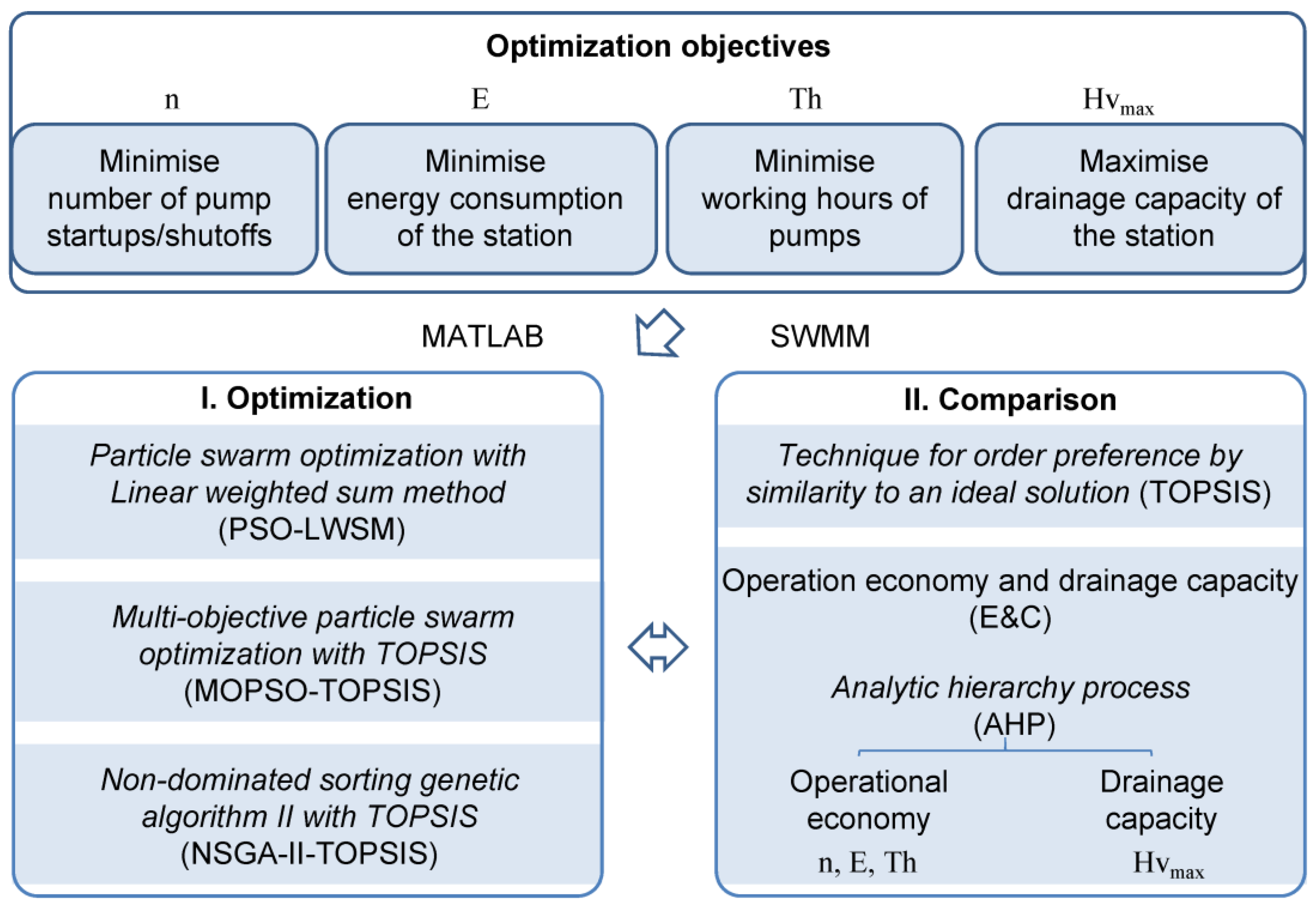
2.1. Optimization Module

2.1.1. Optimization Objectives

In this study, four objectives were selected based on a review of pumping station optimization literature, and the rationale for their selection is given below.

Number of Pump Startups/Shutoffs

Too many startups and shutoffs (n) will affect the service life of pumps and motors, thereby increasing the pump depreciation rate and maintenance costs. Therefore, it is necessary to optimize to reduce the number of times that pumps are started up or shut off.

Energy Consumption of a Pumping Station

As the startup and shutoff depths of pumps are altered, the pump working conditions (flow, head, and efficiency) will change, thus affecting the energy consumption [15,16]. The energy consumption of pumps (E) will increase if the selected startup and shutoff depths are inappropriate or suboptimal.

Working Hours of Pumps

A high operational time will lead to serious wear of pumps [17], thereby increasing the frequency of maintenance/replacement of pumps, reducing the service life, and increasing the maintenance costs. Therefore, the working hour of pumps (Th) is one of the important factors that need to be considered.

Drainage Capacity of a Pumping Station

Alteration of pump operating conditions caused by a change of depth will inevitably affect the drainage capacity of a pumping station [18]. In this study, the drainage capacity of the pumping station is assessed using the maximum depth of the river (${\mathrm{H}}_{{\mathrm{v}}_{\max }}$) rather than the water level after drainage [1]. The highest water levels in the river correspond to the most severe flooding in the drainage area, and the lower the maximum depth of the river is, the lower the severity is. Therefore, the maximum depth of the river is selected as an indicator of the drainage capacity of the pumping station. Minimizing the maximum depth of the river is a key objective; the smaller the value, the better the drainage capacity of the drainage pumping station.

2.1.2. Multi-Objective Optimization Methods

Determination of the Objective Function

Changes to pump startup and shutoff depths have impacts on the number of startups/shutoffs, energy consumption, working hours, and pumping station drainage capacity. In order to explore the impact of startup and shutoff depths on the optimization objectives, other parameters should be kept unchanged while adjusting the startup and shutoff depths (the decision variables). In this way, only the pump startup and shutoff depths affect the optimization objectives. Once pumps in a drainage pumping station start to operate, the water level of the river will generally reduce to the lowest allowable depth. Therefore, this study will optimize only the pump startup depths, and consider the shutoff depths as fixed.

With changes in the pump startup depths, working conditions of the pumps change accordingly and the water level of the river also changes, thus further affecting the working conditions of the pumps. Therefore, it is difficult to directly explore the relationship between the startup depths of pumps and the optimization objectives. As such, the range of startup depths allowed in the optimization is restricted to values between H_min and H_max. The objective function (Equation (1)) is shown below to find the minimum optimization multi-objective value.

$${\mathrm{N}}_{\min }{=\mathrm{minF}(\mathrm{H}}_{\min }{< \mathrm{h}}_{1 }{\dots \mathrm{h}}_{\mathrm{j} }{\dots \mathrm{h}}_{\mathrm{D} }\le { \mathrm{H}}_{\max }),$$

(1)

where $\mathrm{N}$ is the total value of multi-objectives, which can be decomposed into multi-objective values, to achieve the goal of multi-objective optimization; $\mathrm{j}$= (0, 1, 2, …, D), D is the number of pumps in a drainage pumping station; ${\mathrm{H}}_{\max }$ is the maximum allowable pump startup depth; ${\mathrm{H}}_{\min }$ is the minimum allowable pump startup depth.

Particle Swarm Optimization (PSO)

Particle swarm optimization (PSO) is one of the common evolutionary algorithms, which simulates the social dynamics of a flock of birds or fish based on a stochastic population [19]. It is often used to solve optimization problems in various fields, and it also has some application in the optimization of drainage pumping stations [5].

In PSO, the particles in a random swarm seek the optimal solution according to certain criteria. Each particle in the swarm has two groups of parameters, namely location, and velocity, and the particle location is the value of optimization parameters. In this study, the particle locations are the startup depths of the pumps. In the solution space, each particle will change its location depending on its velocity. At each time step in the optimization process, the best location achieved so far is recorded for each particle individually (the individual best positions), along with the best position so far across the whole population (the global best position). The velocity of each particle and its position in each subsequent time step are then determined based on an attraction to both its individual best position and the global best position.

Assuming that each particle searches for the best solution (i.e., the best location) in a D-dimensional solution space, the parameters of the particle are changed according to the following equation [20]:

$$\{\begin{array}{c}{{\mathrm{v}}_{\mathrm{i}}^{\mathrm{j}}}_{{}_{\mathrm{t}+1}}{=\mathrm{w}}_{\mathrm{t}}{ \times \mathrm{v}}_{\mathrm{i}}^{\mathrm{j}}{}_{\mathrm{t}}{+\mathrm{c}}_1 \times {\mathrm{r}}_1{{}_{\mathrm{i}}^{\mathrm{j}}}_{\mathrm{t}}{ \times (\mathrm{Pbest}}_{\mathrm{i}}^{\mathrm{j}}{}_{\mathrm{t} }{- \mathrm{h}}_{\mathrm{i}}^{\mathrm{j}}{}_{\mathrm{t}}{)+\mathrm{c}}_2{ \times \mathrm{r}}_2{{}_{\mathrm{i}}^{\mathrm{j}}}_{\mathrm{t}}{ \times (\mathrm{Gbest}}_{\mathrm{i}}^{\mathrm{j}}{}_{\mathrm{t}}-{ \mathrm{h}}_{\mathrm{i}}^{\mathrm{j}}{}_{\mathrm{t}})\\ {\mathrm{h}}_{\mathrm{i}}^{\mathrm{j}}{}_{\mathrm{t}+1}{=\mathrm{h}}_{\mathrm{i}}^{\mathrm{j}}{}_{\mathrm{t}}{+\mathrm{v}}_{\mathrm{i}}^{\mathrm{j}}{}_{\mathrm{t}+1}\\ {\mathrm{F}}_{\mathrm{i}}^{\mathrm{t}}{=1/\mathrm{N}}_{\mathrm{i}}^{\mathrm{t}}\end{array},$$

(2)

where $\mathrm{h}$ is the location of particles (in this study representing the pump startup depths); $\mathrm{v}$ is the velocity of particles; $\mathrm{Pbest}$ is the individual best position of particles; $\mathrm{Gbest}$ is the global best position of particles; $\mathrm{F}$ is the fitness of particles.$\mathrm{Pbest}$ and $\mathrm{Gbest}$ are selected based on $\mathrm{F}$; ${\mathrm{c}}_1$, ${\mathrm{c}}_2$ are acceleration constants; ${\mathrm{r}}_1$, ${\mathrm{r}}_2$ are random numbers in the range (0, 1); $\mathrm{i}$ = (1, 2, …, R), R is the number of particles in the swarm; $\mathrm{j}$ = (1, 2, …, D), D is the dimension of the solution space where the particles are located (in this study equal to the number of pumps in the drainage pumping station); $\mathrm{t}$ = (0, 1, 2, …, T), T is the upper limit of the number of iterations; $\mathrm{w}$ is inertia weight, the smaller the $\mathrm{w}$ value is, the smaller the change rate of $\mathrm{v}$ is. In the early stages of iteration, particles should search for all potential global optimal solutions in a large range, and in the later stages of iteration, particles should search for global optimal solutions in a small range. Therefore, $\mathrm{w}$ will become smaller and smaller as the number of iterations progresses. In this study, the nonlinear decreasing method (Equation (3)) is adopted to reduce the value of $\mathrm{w}$ [21,22,23].

$${\mathrm{w}}_{\mathrm{t}}{=\mathrm{w}}_{\mathrm{e}}{ \times (\mathrm{w}}_{\mathrm{s}}{/\mathrm{w}}_{\mathrm{e}}{)}^{{1/(1+\mathrm{c}}_{\mathrm{N}} \times \mathrm{t}/\mathrm{T})},$$

(3)

where ${\mathrm{w}}_{\mathrm{s}}$ is the initial inertia weight (usually set to 0.95); ${\mathrm{w}}_{\mathrm{e}}$ is the final inertia weight (usually set to 0.4); ${\mathrm{c}}_{\mathrm{N}}$ is the exponential factor (usually set to 10).

The startup of pumps in the drainage pumping station depends on the depth of the River Yongfeng upstream of the pumping station. When the river depth reaches the pump startup depth, pumps begin to operate; when the river depth reduces to the minimum allowable pump shutoffs depth, pumps stop. When the water level of the river rises due to rainfall, the process will then repeat.

In the process of optimizing the drainage pumping station, pump startup depths should be limited so that the water depth of the River Yongfeng is not too deep when the pumps start. However, since the drainage pumping station pumps are immersed in the River Yongfeng, the pump inflow curves will change with the startup depths. Therefore, it is difficult to obtain the new inflow curves before the startup depths have been altered. It is also difficult to determine the maximum allowable pump startup depth from the inflow and outflow curves. Therefore, this study selects ${\mathrm{H}}_{\max }$ according to the actual operation of a drainage pumping station.

When PSO is used for multi-objective optimization, before optimization the optimal pump startup depth is unknown. In order to satisfy the optimization objectives, it is possible that the startup depth of the pump with the lowest startup depth in the optimal drainage pumping station design will be deeper than the maximum allowable river depth by the end of drainage, thus failing to achieve the best drainage effect. Therefore, the startup depth of the pump with the lowest startup depth in the optimal drainage pumping station is constrained so that it can only be less than or equal to ${\mathrm{He}}_{\mathrm{limit}}$ (i.e., the maximum allowable depth of drainage pumping station by the end of drainage). If the startup depth of the pump with the lowest startup depth in the optimal drainage pumping station in the process of optimization is deeper than the maximum allowable depth of drainage pumping station by the end of drainage, it is set to equal the maximum allowable depth [24]:

$$\{\begin{array}{c}{\mathrm{H}}_{\min }<{ \mathrm{h}}_1{\dots \mathrm{h}}_{\mathrm{j}}{\dots \mathrm{h}}_{\mathrm{D}} \le { \mathrm{H}}_{\max }\\ {\min (\mathrm{h}}_{\mathrm{i}}^{\mathrm{j}}{)}_{\mathrm{t}} \le { \mathrm{He}}_{\mathrm{limit}}\end{array},$$

(4)

wherein, ${\mathrm{He}}_{\mathrm{limit}}$ is the maximum allowable depth of drainage pumping station by the end of drainage. In this way, the limited condition of the pump startup depth is obtained, thus providing the constraint condition of the change rate of river water depth (particle velocity in PSO):

$${\mathrm{H}}_{\min }-{ \mathrm{h}}_{\mathrm{i}}^{\mathrm{j}} <{ \mathrm{v}}_{\mathrm{i}}^{\mathrm{j}} \le { \mathrm{H}}_{\max }-{ \mathrm{h}}_{\mathrm{i}}^{\mathrm{j}},$$

(5)

The particle swarm is initialized according to the above limited conditions (the initial particle location and velocity):

$$\{\begin{array}{c}{\mathrm{h}}_{\mathrm{i}}^{\mathrm{j}}{}_0{=\mathrm{H}}_{\min }{+\mathrm{r}}_3{{}_{\mathrm{i}}^{\mathrm{j}}}_{\mathrm{t}}{ \times (\mathrm{H}}_{\max }-{ \mathrm{H}}_{\min })\\ {\mathrm{v}}_{\mathrm{i}}^{\mathrm{j}}{}_0{=\mathrm{v}}_{\max }{{}_{\mathrm{i}}^{\mathrm{j}}}_0-{ 2 \times \mathrm{r}}_4{{}_{\mathrm{i}}^{\mathrm{j}}}_{\mathrm{t}}{ \times \mathrm{v}}_{\max }{{}_{\mathrm{i}}^{\mathrm{j}}}_0\end{array},$$

(6)

wherein, ${\mathrm{r}}_3$, ${\mathrm{r}}_4$ are random numbers in the range (0, 1); ${\mathrm{v}}_{\max }$ is the absolute value of ${\mathrm{H}}_{\min }-{\mathrm{h}}_{\mathrm{i}}^{\mathrm{j}}$ or ${\mathrm{H}}_{\max }-{\mathrm{h}}_{\mathrm{i}}^{\mathrm{j}}$ in Equation (5). The initial location and velocity of the particle swarm can be obtained by Equation (6). After initializing the particle swarm, the initial data is substituted into the particle swarm optimization to obtain the optimal solution based on fitness.

Linear Weighted Sum Method (LWSM)

To simultaneously deal with four optimization objectives in this study, the linear weighted sum method (LWSM) is adopted to transform multi-objective optimization to single-objective optimization by weighting four objectives. The introduction of weight allows control of which objectives are the most influential in the optimization, so as to obtain different startup water level schemes, using the following formula (Equation (7)).

$$\{\begin{array}{c}{\mathrm{x}}_1{+\mathrm{x}}_2{+\mathrm{x}}_3{+\mathrm{x}}_4=1\\ {\mathrm{N}}_{\mathrm{i}}^{\mathrm{t}}{=\mathrm{x}}_1{ \times \mathrm{N}}_1{}_{\mathrm{i}}^{\mathrm{t}}{+\mathrm{x}}_2{ \times \mathrm{N}}_2{}_{\mathrm{i}}^{\mathrm{t}}{+\mathrm{x}}_3{ \times \mathrm{N}}_3{}_{\mathrm{i}}^{\mathrm{t}}{+\mathrm{x}}_4{ \times \mathrm{N}}_4{}_{\mathrm{i}}^{\mathrm{t}}\end{array},$$

(7)

where ${\mathrm{x}}_1$, ${\mathrm{x}}_2$, ${\mathrm{x}}_3$ and ${\mathrm{x}}_4$ are the weights corresponding to each optimization objective, the corresponding values will be obtained by the analytic hierarchy process (AHP). $\mathrm{N}$ is the total multi-objective value; ${\mathrm{N}}_1$ is the value of the number of pump startup/shutoff objective; ${\mathrm{N}}_2$ is the value of the energy consumption of pumps objective; ${\mathrm{N}}_3$ is the value of working hours of pumps objective; ${\mathrm{N}}_4$ is the value of the capacity of a drainage pumping station objective.

Due to the large numerical differences and different units of the optimization objectives, it is difficult to give weights, so ${\mathrm{N}}_1$, ${\mathrm{N}}_2$, ${\mathrm{N}}_3$, and ${\mathrm{N}}_4$ need to be normalized. The formula (Equation (8)) of normalization is shown below.

$$\{\begin{array}{c}{\mathrm{N}}_1{}_{\mathrm{i}}^{\mathrm{t}}={\displaystyle \sum _{\mathrm{j}=1}^{\mathrm{D}}}{\mathrm{n}}_{\mathrm{t}}{}_{\mathrm{i}}^{\mathrm{j}}{/\mathrm{n}}_{\mathrm{s}}\\ \begin{array}{c}{\mathrm{N}}_2{}_{\mathrm{i}}^{\mathrm{t}}={\displaystyle \sum _{\mathrm{j}=1}^{\mathrm{D}}}{\mathrm{E}}_{\mathrm{t}}{}_{\mathrm{i}}^{\mathrm{j}}{/\mathrm{E}}_{\mathrm{s}}\\ {\mathrm{N}}_3{}_{\mathrm{i}}^{\mathrm{t}}={\displaystyle \sum _{\mathrm{j}=1}^{\mathrm{D}}}{\mathrm{Th}}_{\mathrm{t}}{}_{\mathrm{i}}^{\mathrm{j}}{/\mathrm{Th}}_{\mathrm{s}}\\ {\mathrm{N}}_4{}_{\mathrm{i}}^{\mathrm{t}}{=\mathrm{Hv}}_{\max }{{}_{\mathrm{t}}}_{\mathrm{i}}{{/\mathrm{Hv}}_{\max }}_{{}_{\mathrm{s}}}\end{array}\end{array},$$

(8)

where ${\mathrm{n}}_{\mathrm{t}}{}_{\mathrm{i}}^{\mathrm{j}}$ is the number of startups/shutoffs of a single pump; ${\mathrm{n}}_{\mathrm{s}}$ is the number of startups/shutoffs before optimization; ${\mathrm{E}}_{\mathrm{t}}{}_{\mathrm{i}}^{\mathrm{j}}$ is the energy consumption of a single pump; ${\mathrm{E}}_{\mathrm{s}}$ is the modelled energy consumption of the pumping station before optimization; ${\mathrm{Th}}_{\mathrm{t}}{}_{\mathrm{i}}^{\mathrm{j}}$ is the working hours of a single pump; ${\mathrm{Th}}_{\mathrm{s}}$ is the working hours of pumps before optimization; ${\mathrm{Hv}}_{\max }{{}_{\mathrm{t}}}_{\mathrm{i}}$ is the maximum depth of the river at the time of drainage; ${{\mathrm{Hv}}_{\max }}_{{}_{\mathrm{s}}}$ is the maximum depth of the river before optimization.

Analytic Hierarchy Process (AHP)

In LWSM introduced above, ${\mathrm{x}}_1$, ${\mathrm{x}}_2$, ${\mathrm{x}}_3$, and ${\mathrm{x}}_4$ are unknown and need to be determined. In this study, the analytic hierarchy process (AHP) [25] is adopted to determine the weights, allowing pumping station staff to provide scores based on their perspectives of operational economy and drainage capacity. The weights (${\mathrm{x}}_1$, ${\mathrm{x}}_2$, ${\mathrm{x}}_3$, and ${\mathrm{x}}_4$) of ${\mathrm{N}}_1$, ${\mathrm{N}}_2$, ${\mathrm{N}}_3$, and ${\mathrm{N}}_4$ are obtained by using the comparison matrix of AHP.

Multi-Objective Particle Swarm Optimization (MOPSO)

Compared to PSO, multi-objective particle swarm optimization (MOPSO) uses the concept of Pareto dominance to determine the flight direction of a particle, and it maintains non-dominated solutions found previously in a global repository that is later used by other particles to guide their flight [26].

Therefore, the difference between MOPSO and PSO is the selection of the personal and global best positions, as well as a global repository for storing generations of non-dominated solutions. The particle information contained in the global repository of each generation is the optimization result of each generation. The search for the personal best position in MOPSO is to judge each particle and randomly select a non-dominated solution from the swarm composed of successive iterations of each particle as the personal best position. For the global optimal location, it is to judge the global repository of each generation and select the one with the larger crowding distance as the global best position [27,28].

MOPSO builds a global repository based on non-dominated solutions of each generation, copies non-dominated solutions of each generation to the global repository, and then carries out non-dominated screening within the global repository. If the size of the global repository after screening exceeds the predetermined size, it will be screened according to the crowding distance, and the particles with a high crowding distance will be retained. Finally, the optimization results can be obtained through multiple iterations to output the global repository. The number of MOPSO runs (generations) is consistent with that of PSO-LWSM.

Non-Dominated Sorting Genetic Algorithm II (NSGA-II)

The non-dominated sorting genetic algorithm II (NSGA-II) is first used to optimize control strategy [29], since it is computationally fast and has been shown to provide better coverage and maintain a better spread of solutions than other multi-objective evolutionary algorithms (MOEAs) [29,30].

In NSGA-II, parent organisms and child organisms are merged (the child organisms are formed by the hybridization and variation of the parent organisms) prior to fast non-dominated sorting. Then, the crowding distance of each individual in the non-dominated layer is sorted. Finally, the first few layers which retain the non-dominated solution form the final child organisms with the individuals with larger crowding distance, and will become the parent organisms of the next iteration. The optimization results are achieved through continuous iteration. The number of NSGA-II runs (generations) is consistent with that of PSO-LWSM.

Technique for Order Preference by Similarity to an Ideal Solution (TOPSIS)

Multi-criteria decision analysis (MCDA) allows decision-makers to include a full range of indicators. There are many MCDA methods, such as AHP, TOPSIS, etc. [31].

To help the staff of a pumping station to select a better solution that can be implemented from a non-dominated solution set obtained in each iteration, and to avoid the subjectivity as far as possible in the selection, this paper uses TOPSIS [32] to sort the non-dominated solution set, and the top one is considered the optimization result.

Since each iteration of NSGA-II or MOPSO will generate a set of Pareto frontier solutions, this paper uses TOPSIS to get the best solution from these frontier solutions obtained by NSGA-II or MOPSO as the optimization result of each iteration, and compares this with PSO-LWSM later using the comparison module. The approaches that combine NSGA-II and MOPSO with TOPSIS are called NSGA-II-TOPSIS and MOPSO-TOPSIS respectively.

The Initial Conditions of the Pumping System Model

The initial energy consumption of pumps for the pumping system model is evaluated based on the actual annual drainage volume of the drainage pumping station (Q_y), modelled drainage volume and the electricity use of the drainage pumping station due to pumps lifting water (E_n). A fixed (i.e., independent of time of use) electricity price is adopted in the study to reduce uncertainty and computational workload, since the time of day at which a rainfall event occurs is unknown. In addition, the number of pump startups/shutoffs, working hours, and the maximum depth of the river can be reduced as far as possible by manually adjusting the startup depths of the pumps, under the condition that the energy consumption of the model is as close as possible to the actual energy consumption. Then the startup/shutoff scheme of pumps obtained is regarded as the initial one before optimization. Thus, the operating conditions before optimization are obtained.

2.2. Comparison Module

The comparison module includes two comparisons: TOPSIS comparison (representing objectivity), and operational economy and drainage capacity (E&C) comparison using AHP (representing subjectivity), to ensure the reliability of the optimal results.

2.2.1. TOPSIS Comparison

This comparison uses TOPSIS to sort the optimization results of MOPSO-TOPSIS and NSGA-II-TOPSIS with the optimization results of PSO-LWSM to get a comprehensive evaluation index for the corresponding algorithms, to complete the comparison of each algorithm.

2.2.2. Operational Economy and Drainage Capacity (E&C) Comparison

This module aims to calculate the economic loss caused by a single startup/shutoff of the pump and the pump unit operating time. Then, combined with the local electricity price to calculate the corresponding economic loss resulting from pump energy consumption, this provides the economic loss of the corresponding optimization results. Then, the drainage capacity is incorporated into the AHP comparison matrix to get the weight of the corresponding objective. Finally, the comprehensive evaluation value of the corresponding optimization result is calculated by combining the weight obtained with the objectives index, and the quality of the system optimization result is determined by comparing the size of the corresponding comprehensive evaluation index. The specific process is as follows.

Evaluation from the Operational Economy Perspective

The objective values considered for the operational economy are ${\mathrm{N}}_1$, ${\mathrm{N}}_2$ and ${\mathrm{N}}_3$. The electricity consumption (loss) of ${\mathrm{N}}_2$ is easily obtained, while the economic impact of ${\mathrm{N}}_1$ and ${\mathrm{N}}_3$ on the pumping station is not easy to figure out. In this study, the economic losses caused by ${\mathrm{N}}_1$, ${\mathrm{N}}_2$ and ${\mathrm{N}}_3$ are calculated as follows (Equation (9)).

$$\{\begin{array}{c}\begin{array}{c}{{\mathrm{S}}_1}_{{}_{\mathrm{t}}}={\displaystyle \sum _{\mathrm{j}=1}^{\mathrm{D}}}{\mathrm{n}}_{\mathrm{t}}^{\mathrm{j}}{ \times \mathrm{s}}_1\\ {{\mathrm{S}}_2}_{{}_{\mathrm{t}}}={\displaystyle \sum _{\mathrm{j}=1}^{\mathrm{D}}}{\mathrm{E}}_{\mathrm{t}}^{\mathrm{j}} \times \mathrm{e}\\ {{\mathrm{S}}_3}_{{}_{\mathrm{t}}}={\displaystyle \sum _{\mathrm{j}=1}^{\mathrm{D}}}{\mathrm{Th}}_{\mathrm{t}}^{\mathrm{j}}{ \times \mathrm{s}}_3\end{array}\end{array},$$

(9)

where ${\mathrm{S}}_1$ is the economic loss caused by pump startups/shutoffs; ${\mathrm{s}}_1$ is the economic loss caused by one start of a pump; ${\mathrm{S}}_2$ is the electricity fee paid by the pumping station due to the energy consumption of pumps; $\mathrm{e}$ is the electricity price; ${\mathrm{S}}_3$ is the economic loss caused by wear caused by the operation of pumps; ${\mathrm{s}}_3$ is the hourly economic loss due to pump wear. The values of ${\mathrm{s}}_1$ and ${\mathrm{s}}_3$ are determined as below (Equation (10)).

$$\{\begin{array}{c}{\mathrm{s}}_1{=\mathrm{sy}}_1{/\mathrm{n}}_0\\ {\mathrm{s}}_3{=\mathrm{sy}}_3{/\mathrm{Th}}_0\end{array},$$

(10)

where ${\mathrm{s}}_1$ is the economic loss caused by each start of the pump; ${\mathrm{sy}}_1$ is the economic loss caused by the pump startups/shutoffs before optimization; ${\mathrm{n}}_0$ is the average number of pump startups/shutoffs of the initial swarm; ${\mathrm{s}}_3$ is the economic loss per hour of pump operation; ${\mathrm{sy}}_3$ is the economic loss of the drainage pumping station caused by the wear of the pumps during operation; ${\mathrm{Th}}_0$ is the average working hours of pumps of the initial swarm. ${\mathrm{sy}}_1$ and ${\mathrm{sy}}_3$ are generally not recorded in drainage pumping stations, so ${\mathrm{sy}}_1$ and ${\mathrm{sy}}_3$ are computed through the following formula (Equation (11)):

$$\{\begin{array}{c}{\mathrm{sy}}_1{=(\mathrm{x}}_1{/(\mathrm{x}}_1{+\mathrm{x}}_3{\left)\right) \times \mathrm{Q}}_{\mathrm{n}}{ \times (\mathrm{S}}_{\mathrm{y}}-{ \mathrm{S}}_{\mathrm{b}}{)/\mathrm{Q}}_{\mathrm{y}}\\ {\mathrm{sy}}_3{=(\mathrm{x}}_3{/(\mathrm{x}}_1{+\mathrm{x}}_3{\left)\right) \times \mathrm{Q}}_{\mathrm{n}}{ \times (\mathrm{S}}_{\mathrm{y} }-{ \mathrm{S}}_{\mathrm{b}}{)/\mathrm{Q}}_{\mathrm{y}}\end{array},$$

(11)

where ${\mathrm{S}}_{\mathrm{y}}$ is the total economic loss caused by pumps maintenance in a multi-year average year in a drainage pumping station; ${\mathrm{S}}_{\mathrm{b}}$ is the economic loss caused by the rust of pumps in ${\mathrm{S}}_{\mathrm{y}}$; ${(\mathrm{S}}_{\mathrm{y}}-{ \mathrm{S}}_{\mathrm{b}})$ is the average annual economic loss caused by the pump start-ups/shutoffs and operation wear; ${\mathrm{Q}}_{\mathrm{y}}$ is the average annual total drainage volume of the drainage pumping station; ${\mathrm{Q}}_{\mathrm{n}}$ is the drainage volume in the scenario; ${\mathrm{Q}}_{\mathrm{n}}{ \times (\mathrm{S}}_{\mathrm{y}}-{ \mathrm{S}}_{\mathrm{b}}{)/\mathrm{Q}}_{\mathrm{y}}$ is the economic loss caused by the pump startups/shutoffs and operation wear in this scenario. By weighting them respectively, the values of ${\mathrm{sy}}_1$ and ${\mathrm{sy}}_3$ can be obtained. ${\mathrm{sy}}_1$ and ${\mathrm{sy}}_3$ of different return periods can be obtained by ${\mathrm{Q}}_{\mathrm{n}}$ of different return periods.

Comprehensive Evaluation of the Operational Economy and Drainage Capacity

The following formula is used for comprehensive evaluation of the operational economy and drainage capacity (E&C) of the pumping station:

$${\mathrm{S}}_{\mathrm{a}}{}_{\mathrm{t}}{=(\mathrm{x}}_1{+\mathrm{x}}_2{+\mathrm{x}}_3) \times ({{\mathrm{S}}_1}_{{}_{\mathrm{t}}}+{{\mathrm{S}}_2}_{{}_{\mathrm{t}}}+{{\mathrm{S}}_3}_{{}_{\mathrm{t}}})/({{\mathrm{S}}_1}_{{}_0}+{{\mathrm{S}}_2}_{{}_0}+{{\mathrm{S}}_3}_{{}_0}{)+\mathrm{x}}_4{{ \times \mathrm{Hv}}_{\max }}_{{}_{\mathrm{t}}}{{/\mathrm{Hv}}_{\max }}_{{}_0},$$

(12)

where ${\mathrm{S}}_{\mathrm{a}}$ is the comprehensive evaluation value of the pumping station from the two aspects of operational economy and drainage capacity (E&C comprehensive evaluation index). The smaller ${\mathrm{S}}_{\mathrm{a}}$ is, the better the optimization solution is.

2.3. Sensitivity Analysis

To test the influence of the selection of weight values in PSO-LWSM on the final optimization results, this paper adopts the perturbation method for sensitivity analysis of weight values, and the perturbation interval is (${\mathrm{x}}_{\mathrm{n}}$ × 0.8, ${\mathrm{x}}_{\mathrm{n}}$ × 1.2) (n = 1, 2, 3 and 4) [33]. To simplify the analysis, when a weight of ${\mathrm{x}}_1$−${ \mathrm{x}}_4$ increases or decreases according to the change of disturbance value, the rest weights increase or decrease equally.

3. Case Study

3.1. Study Area

The study area called the Xiaohekou case is located in Ma’anshan city, Anhui province, China, and has a monsoon climate. The average annual temperature is 16.0 °C, and the average annual rainfall is 1100 mm. July is the month with the heaviest rainfall of the year, with a total rainfall of about 182.5 mm. The drainage pumping station service covers an area of 13.2 ${\mathrm{km}}^2$. The water system in the drainage area is complex, river and lakes cross, river depths are 2 to 3 m, and the ground elevation is about 10 m.

The whole flow route is surface runoff → underground storm sewers → the River Yongfeng → the pumping station → the River Caishi. The drainage pumping station was built on the River Yongfeng. The River flows from north to south, and the downstream is the River Caishi which flows from east to west. During wet weather, when flood water levels are higher, the pumping station pumps water from the River Yongfeng to the River Caishi.

The drainage area is divided into 623 sub-catchments (Figure 2). The drainage system includes underground storm sewers, rivers, lakes, and a pumping station. Storm sewers are designed to convey runoff from a one-year design storm to satisfy local design standards.

3.2. System Modelling and the Parameters of the Drainage Pumping Station

In order to simulate the operation of the drainage pumping station, the open-source software package, SWMM, which is widely used around the world, is used. The system includes 623 subcatchments, 431 junctions, 434 conduits (including river channels), 3 storage units representing lakes, and 1 drainage pumping station (including 1 storage unit, 11 pumps, and 11 outfalls). The type 3 pump curve (head-flow) is used for pumps. The rainfall time series are produced by the Chicago hyetograph method according to the Ma’anshan rainfall intensity formula, with a storm peak coefficient of 0.4, rainfall duration of 2 h, and return period of 30 years (the maximum drainage standard for the pumping station in this area). Return periods of 5, 10, 50, and 100 years are also modelled to find the influence on the results of three optimization approaches.

The parameters of the drainage pumping station (

Table 1. The parameters of the drainage pumping station.

The Parameters of the Drainage Pumping Station
Drainage pumping station	Area occupied by the pumping station (km2)	13.2
	Bottom elevation of the River Yongfeng (m)	3.2
	Normal elevation of the River Yongfeng (m)	5.2
	Maximum depth of the River Yongfeng (m)	7.5
	Bottom elevation of the River Caishi (m)	3.2
	Normal elevation of the River Caishi (m)	7.2
	Maximum depth of the River Caishi (m)	10
	Elevation of the outlet (m)	10.5
	Maximum allowable depth of the pumping station by the end of drainage (m) (${\mathrm{He}}_{\mathrm{limit}}$)	4.9
Pumps	Number of pumps	11
	Total flow of pumps (m3/s)	58.12
	Maximum startup depth of pumps (m) (${\mathrm{H}}_{\max }$)	6.6
	Shutoff depth of pumps (m) (${\mathrm{H}}_{\min }$)	4.1

) in the SWMM-model are determined according to the actual parameters of the station. The water level variation of the River Caishi at the location of the drainage pumping station is unknown since there are so many water systems flowing into the upper reaches of the River Caishi that it is difficult to determine its water level. However, the water does not generally flood the outfall to the River Caishi. Therefore, this system does not consider the inundation of the outfall, and the head of pumps in the pumping station is calculated as the difference between the elevation at the bottom of the outfall and the water level of the River Yongfeng at the location of the drainage pumping station.

The initial values of optimization objectives and economic loss can be obtained from the actual economic loss and operation of the pumping station (

Table 2. Values of the evaluated parameters.

Parameter		Value
Qy	Average annual total drainage volume of the drainage pumping station (m3)	8 × 108
En	Average electricity use by the pumping station due to the pumps lifting water (CNY)	7.6 × 107
e	Electricity price (CNY/(Kw·h))	0.6324
Sy	Total economic loss caused by pump maintenance in a multi-year average year in the drainage pumping station (CNY)	6 × 107
Sb	Economic loss caused by the rust of the pumps in Sy (CNY)	1.5 × 107

).

3.3. AHP Comparison Matrix and Weights

The AHP comparison matrix given by the pump station staff for the case study is shown in

Table 3. Comparison matrix and weights of four objectives.

Comparison Matrix and Weight
	x1	x2	x3	x4
x1	1	1/4	1/2	1
x2	4	1	5/2	3
x3	2	2/5	1	2
x4	1	1/3	1/2	1
weight	0.126	0.497	0.240	0.137

. A consistency test of the comparison matrix is carried out and passed. The weight of each objective is determined by the comparison matrix. They will be used for the PSO-LWSM approach and E&C Comparison module.

4. Results and Discussion

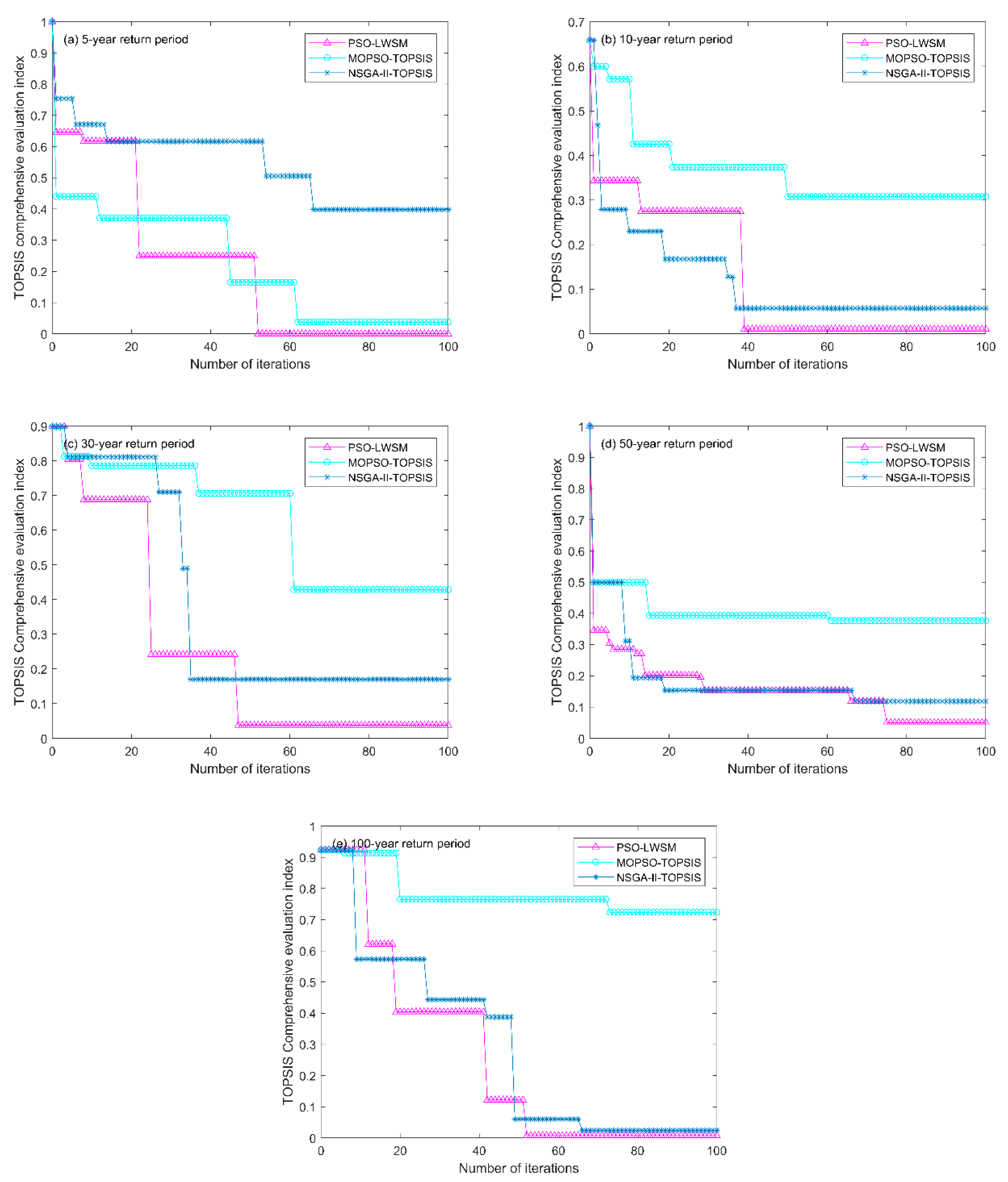
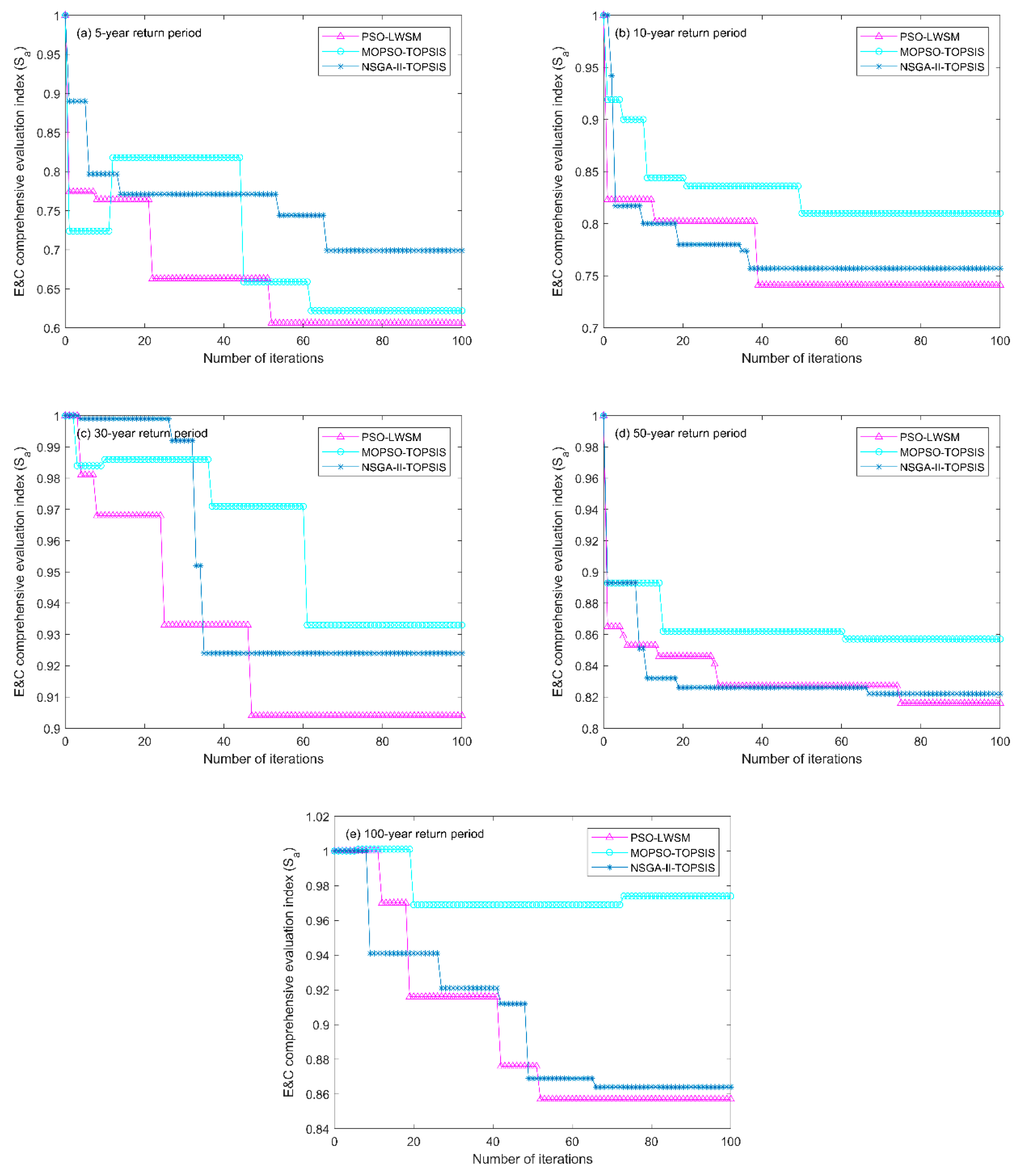
4.1. Optimization Results

Table 4. Optimization results after 100 generations using three approaches.

Return Period (Years)	Optimization Objectives	Before Optimization	PSO-LWSM	MOPSO-TOPSIS	NSGA-II-TOPSIS
5	Number of pump startups/shutoffs	65	14	16	37
	Energy consumption of the pumping station (Kw·h)	8854.83	6334.24	6351.71	6361.1
	Working hours of pumps (h)	32.67	21.78	22.12	22
	Maximum depth of the river (m)	5.36	5.23	5.25	5.34
10	Number of pump startups/shutoffs	648	429	594	452
	Energy consumption of the pumping station (Kw·h)	9194.34	6867.2	6853.61	6995.87
	Working hours of pumps (h)	32.87	23.98	23.75	24.27
	Maximum depth of the river (m)	6.51	5.84	6.32	5.86
30	Number of pump startups/shutoffs	927	623	753	671
	Energy consumption of the pumping station (Kw·h)	9895.34	7841.64	7939.3	7902.73
	Working hours of pumps (h)	33.8	27.71	27.98	28
	Maximum depth of the river (m)	6.91	6.35	5.68	6.37
50	Number of pump startups/shutoffs	813	601	752	640
	Energy consumption of the pumping station (Kw·h)	10,243.22	8350.66	8263.08	8302.5
	Working hours of pumps (h)	36.93	29.87	29.27	29.41
	Maximum depth of the river (m)	6.58	6.27	6.56	6.34
100	Number of pump startups/shutoffs	618	300	530	298
	Energy consumption of the pumping station (Kw·h)	10,878.99	8872.16	9032.58	8967.95
	Working hours of pumps (h)	37.16	32.02	33.01	32.34
	Maximum depth of the river (m)	6.66	5.67	6.1	5.75

shows the final optimization results (100 generations) of three approaches (PSO-LSWM, MOPSO-TOPSIS, and NSGA-II-TOPSIS) in the optimization module under different return periods of design storm in the case study. It can be seen that no matter which approach is used, most of the multi-objective optimizations of the drainage pumping station will lead to better results (than with no optimization). Due to multiple objectives, it is still difficult to judge which approach is the best. For this reason, the comparison module in the proposed framework will be used next.

4.2. Comparison Results

4.2.1. TOPSIS Comparison Results

Using TOPSIS to compare the optimization results, the comparison results (TOPSIS comprehensive evaluation index) of the three approaches can be obtained. Figure 3 shows the TOPSIS comparison results of the three approaches in the optimization module after 10,000 SWMM simulations (100 population × 100 generation) [34] for each return period. From Figure 3, we can see the convergence generation for each approach and the quality of the optimization results. All three approaches converge gradually in stages to the best optimization results before the number of iterations reaches in terms of convergence rate, when the return periods are 10, 30, and 50 years, NSGA-II-TOPSIS is faster than PSO-LWSM, while under other return periods, PSO-LWSM is faster than NSGA-II-TOPSIS. The convergence rate of MOPSO-TOPSIS is faster than that of PSO-LWSM when the return period is 50 years, while under other return periods, PSO-LWSM is faster than MOPSO-TOPSIS. The averaged values of the TOPSIS comprehensive evaluation index of the three approaches under different return periods are 0.021, 0.154, and 0.375, respectively. A smaller index indicates a better approach. In terms of optimization results (TOPSIS comprehensive evaluation index), PSO-LWSM is better than NSGA-II-TOPSIS and MOPSO-TOPSIS under all return periods.

4.2.2. E&C Comparison Results

Using E&C to compare the optimization results of the three approaches, the following comparison results can be obtained (Figure 4).

It can be seen from Figure 4 that the E&C comparison results of PSO-LWSM are still better than those of NSGA-II-TOPSIS and MOPSO-TOPSIS, although AHP is used to give subjective weights here (Table 3).

The averaged values of the E&C comprehensive evaluation index of PSO-LWSM, NSGA-II-TOPSIS, and MOPSO-TOPSIS under different return periods after optimization are 0.785, 0.813, and 0.839, respectively. Based on Figure 3 and Figure 4, and Table 4, no matter how the three approaches are compared, the optimization results of PSO-LWSM are better than those of NSGA-II-TOPSIS and MOPSO-TOPSIS in this case study.

4.2.3. Sensitivity Analysis Results

The complete results of sensitivity analysis are provided in the Supplementary Information (Tables S1–S5 and Figures S1–S3) considering the length of the paper. Through sensitivity analysis, it can be seen that the order of sensitivity of four optimization objectives from high to low is $\mathrm{n}$ > $\mathrm{Th}$ > $\mathrm{E}$ > ${\mathrm{Hv}}_{\max }$. Although altering the weight values may cause the changes of PSO-LWSM optimization results, the obtained results are still better than those of NSGA-II-TOPSIS and MOPSO-TOPSIS.

Based on the sensitivity analysis results, objectives with higher sensitivity should choose relatively lower weights when using AHP, to ensure stability of the optimization results. Furthermore, from the perspective of operational economy, the weights of n, E and Th should be raised. Considering that the sensitivity of $\mathrm{E}$ is lower than that of $\mathrm{Th}$, and the sensitivity of $\mathrm{E}$, $\mathrm{Th}$ and ${\mathrm{Hv}}_{\max }$ is much lower than that of $\mathrm{n}$, the weights of the four objectives should be $\mathrm{E}$ > $\mathrm{Th}$ > ${\mathrm{Hv}}_{\max }$ > $\mathrm{n}$ when using PSO-LWSM. The AHP weight selection scheme in this paper obeys this principle.

These results validate the efficiency of the proposed framework. The framework can also be applied to any other objectives with different optimization approaches in the optimization module for a pumping system to reduce energy consumption and maintenance costs. From the point of view of the framework itself, there are no barriers to applying this framework to other optimisation problems. Further verification work will be carried out in other areas in future, providing additional support to the conclusions.

5. Conclusions

In this study, a framework for comparing multi-objective optimization approaches for a stormwater drainage pumping system is proposed, which consists of two modules, the optimization module, and the comparison module. It integrates four optimization objectives based on the number of pump startups/shutoffs, energy consumption, working hours, and drainage capacity. Three optimization approaches, PSO-LWSM, MOPSO-TOPSIS, and NSGA-II-TOPSIS, are used and compared under different return periods. The Xiaohekou case in Ma’anshan city, China is presented to validate this framework.

The results show that the framework is feasible and has achieved a good optimization solution. The optimization performance of PSO-LWSM is better than that of the NSGA-II-TOPSIS and MOPSO-TOPSIS in the Xiaohekou case. The proposed framework in this study enables easy quantification of the objectives for multi-objective optimization and can be used to optimize and compare the operational economy and drainage capacity of drainage pumping stations. In further study, the overall economic loss of the whole drainage system may be considered from other factors such as the duration of flooding at nodes to provide comprehensive optimization support for a pumping system.

References

1. Yazdi, J.; Choi, H.S.; Kim, J.H. A Methodology for Optimal Operation of Pumping Stations in Urban Drainage Systems. J. Hydro-Environ. Res. 2016, 11, 101–112. [Google Scholar] [CrossRef]
2. Dottori, F.; Szewczyk, W.; Ciscar, J.C.; Zhao, F.; Alfieri, L.; Hirabayashi, Y.; Bianchi, A.; Mongelli, I.; Frieler, K.; Betts, R.A.; et al. Increased Human and Economic Losses from River Flooding with Anthropogenic Warming. Nat. Clim. Chang. 2018, 8, 781–786. [Google Scholar] [CrossRef]
3. Jongman, B. Effective Adaptation to Rising Flood Risk. Nat. Commun. 2018, 9, 1986. [Google Scholar] [CrossRef] [PubMed] [Green Version]
4. Ward, P.J.; Jongman, B.; Aerts, J.C.J.H.; Bates, P.D.; Botzen, W.J.W.; Diaz Loaiza, A.; Hallegatte, S.; Kind, J.M.; Kwadijk, J.; Scussolini, P.; et al. A Global Framework for Future Costs and Benefits of River-Flood Protection in Urban Areas. Nat. Clim. Chang. 2017, 7, 642–646. [Google Scholar] [CrossRef]
5. Wang, H.; Lei, X.; Khu, S.-T.; Song, L. Optimization of Pump Start-Up Depth in Drainage Pumping Station Based on SWMM and PSO. Water 2019, 11, 1002. [Google Scholar] [CrossRef] [Green Version]
6. Al-Ani, D.; Habibi, S. Optimal Pump Operation for Water Distribution Systems Using a New Multi-Agent Particle Swarm Optimization Technique with EPANET. In Proceedings of the 2012 25th IEEE Canadian Conference on Electrical and Computer Engineering (CCECE), Montreal, QC, Canada, 29 April–2 May 2012; pp. 1–6. [Google Scholar]
7. Hou, J.; Li, C.; Tian, Z.; Xu, Y.; Lai, X.; Zhang, N.; Zheng, T.; Wu, W. Multi-Objective Optimization of Start-up Strategy for Pumped Storage Units. Energies 2018, 11, 1141. [Google Scholar] [CrossRef] [Green Version]
8. Yang, S.-N.; Chang, L.-C.; Chang, F.-J. AI-Based Design of Urban Stormwater Detention Facilities Accounting for Carryover Storage. J. Hydrol. 2019, 575, 1111–1122. [Google Scholar] [CrossRef]
9. Dadar, S.; Đurin, B.; Alamatian, E.; Plantak, L. Impact of the Pumping Regime on Electricity Cost Savings in Urban Water Supply System. Water 2021, 13, 1141. [Google Scholar] [CrossRef]
10. Hwang, Y.K.; Kwon, S.H.; Lee, E.H.; Kim, J.H. Development of Optimal Pump Operation Method for Urban Drainage Systems. In Advances in Harmony Search, Soft Computing and Applications; Kim, J.H., Geem, Z.W., Jung, D., Yoo, D.G., Yadav, A., Eds.; Springer: Cham, Switzerland, 2020; pp. 63–69. [Google Scholar]
11. Saliba, S.M.; Bowes, B.D.; Adams, S.; Beling, P.A.; Goodall, J.L. Deep Reinforcement Learning with Uncertain Data for Real-Time Stormwater System Control and Flood Mitigation. Water 2020, 12, 3222. [Google Scholar] [CrossRef]
12. Lu, H.; Ma, X. Hybrid Decision Tree-Based Machine Learning Models for Short-Term Water Quality Prediction. Chemosphere 2020, 249, 126169. [Google Scholar] [CrossRef]
13. Melesse, A.M.; Khosravi, K.; Tiefenbacher, J.P.; Heddam, S.; Kim, S.; Mosavi, A.; Pham, B.T. River Water Salinity Prediction Using Hybrid Machine Learning Models. Water 2020, 12, 2951. [Google Scholar] [CrossRef]
14. Kadkhodazadeh, M.; Farzin, S. A Novel LSSVM Model Integrated with GBO Algorithm to Assessment of Water Quality Parameters. Water Resour. Manag. 2021, 35, 3939–3968. [Google Scholar] [CrossRef]
15. Liu, J.S.; Cheng, J.L.; Gong, Y. Study on Optimal Scheduling Methods of Urban Drainage Pumping Stations Based on Orthogonal Test. Appl. Mech. Mater. 2013, 373–375, 2169–2174. [Google Scholar] [CrossRef]
16. Torregrossa, D.; Capitanescu, F. Optimization Models to Save Energy and Enlarge the Operational Life of Water Pumping Systems. J. Clean. Prod. 2019, 213, 89–98. [Google Scholar] [CrossRef]
17. Fecarotta, O.; Martino, R.; Morani, M.C. Wastewater Pump Control under Mechanical Wear. Water 2019, 11, 1210. [Google Scholar] [CrossRef] [Green Version]
18. Kanno, H. Inside One of Largest Capacity Drainage Pump Stations in the World. World Pumps 2007, 2007, 14–15. [Google Scholar] [CrossRef]
19. Kennedy, J.; Eberhart, R. Particle Swarm Optimization. In Proceedings of the ICNN’95—International Conference on Neural Networks, Perth, Australia, 27 November–1 December 1995; Volume 4, pp. 1942–1948. [Google Scholar]
20. Plimpton, S. Fast Parallel Algorithms for Short-Range Molecular Dynamics. J. Comput. Phys. 1995, 117, 1–19. [Google Scholar] [CrossRef] [Green Version]
21. Feizi, A.E.; Niksokhan, M.H.; Ardestani, M. Multi-Objective Waste Load Allocation in River System by MOPSO Algorithm. Int. J. Environ. Res. 2015, 9, 69–76. [Google Scholar] [CrossRef]
22. Li, Y.; Zhan, Z.-H.; Lin, S.; Zhang, J.; Luo, X. Competitive and Cooperative Particle Swarm Optimization with Information Sharing Mechanism for Global Optimization Problems. Inf. Sci. 2015, 293, 370–382. [Google Scholar] [CrossRef]
23. Shi, Y.; Obaiahnahatti, B.G. Empirical Study of Particle Swarm Optimization. Proc. IEEE Congr. Evol. Comput. 1999, 3, 101–106. [Google Scholar]
24. Wang, H.; Zhang, Y.; Tang, Y.; Liu, Y.; Li, K. Optimization of Pump Start-Stops in Rainwater Pump Station. Harbin Gongye Daxue Xuebao/J. Harbin Inst. Technol. 2017, 49, 98–103. [Google Scholar] [CrossRef]
25. Saaty, T.L. Exploring the Interface between Hierarchies, Multiple Objectives and Fuzzy Sets. Fuzzy Sets Syst. 1978, 1, 57–68. [Google Scholar] [CrossRef]
26. Coello Coello, C.A.; Lechuga, M.S. MOPSO: A Proposal for Multiple Objective Particle Swarm Optimization. In Proceedings of the 2002 Congress on Evolutionary Computation. CEC’02 (Cat. No. 02TH8600), Honolulu, HI, USA, 12–17 May 2002; Volume 2, pp. 1051–1056. [Google Scholar]
27. Coello Coello, C.A.; Pulido, G.T.; Lechuga, M.S. Handling Multiple Objectives with Particle Swarm Optimization. IEEE Trans. Evol. Comput. 2004, 8, 256–279. [Google Scholar] [CrossRef]
28. Fallah-Mehdipour, E.; Haddad, O.B.; Mariño, M.A. MOPSO Algorithm and Its Application in Multipurpose Multireservoir Operations. J. Hydroinform. 2011, 13, 794–811. [Google Scholar] [CrossRef] [Green Version]
29. Deb, K.; Pratap, A.; Agarwal, S.; Meyarivan, T. A Fast and Elitist Multiobjective Genetic Algorithm: NSGA-II. IEEE Trans. Evol. Comput. 2002, 6, 182–197. [Google Scholar] [CrossRef] [Green Version]
30. Sweetapple, C.; Fu, G.; Butler, D. Multi-Objective Optimisation of Wastewater Treatment Plant Control to Reduce Greenhouse Gas Emissions. Water Res. 2014, 55, 52–62. [Google Scholar] [CrossRef] [Green Version]
31. Huang, I.B.; Keisler, J.; Linkov, I. Multi-Criteria Decision Analysis in Environmental Sciences: Ten Years of Applications and Trends. Sci. Total Environ. 2011, 409, 3578–3594. [Google Scholar] [CrossRef]
32. Yoon, P.; Hwang, C.-L. Multiple Attribute Decision Making, an Introduction; Sage Publications: Thousand Oaks, CA, USA, 1995; Volume 104. [Google Scholar]
33. Wang, M.; Sun, Y.; Sweetapple, C. Optimization of Storage Tank Locations in an Urban Stormwater Drainage System Using a Two-Stage Approach. J. Environ. Manag. 2017, 204, 31–38. [Google Scholar] [CrossRef]
34. Yang, Y.; Zhang, T.; Yi, W.; Kong, L.; Li, X.; Wang, B.; Yang, X. Deployment of Multistatic Radar System Using Multi-Objective Particle Swarm Optimisation. IET Radar Sonar Navig. 2018, 12, 485–493. [Google Scholar] [CrossRef]
Figure 1. Framework for comparing optimization approaches for stormwater drainage pumping systems.
Water 14 01248 g001
Figure 2. The SWMM model for the study area. The red rectangle in the figure is the location of the drainage pumping station.
Water 14 01248 g002
Figure 3. Results using TOPSIS Comparison for each generation of three approaches under different return periods: (a) 5-year return period; (b) 10-year return period; (c) 30-year return period; (d) 50-year return period; (e) 100-year return period.
Water 14 01248 g003
Figure 4. Results of the E&C comparison for each generation of three approaches under different return periods: (a) 5-year return period; (b) 10-year return period; (c) 30-year return period; (d) 50-year return period; (e) 100-year return period.
Water 14 01248 g004