Decision Making Model for Municipal Wastewater Conventional Secondary Treatment with Bayesian Networks

Abstract

Technical, economic, regulatory, environmental, and social and political interests make the process of selecting an appropriate wastewater treatment technology complex. Although this problem has already been addressed from the dimensioning approach, our proposal in this research, a model of decision making for conventional secondary treatment of municipal wastewater through continuous-discrete, non-parametric Bayesian networks was developed. The most suitable network was structured in unit processes, independent of each other. Validation, with data in a mostly Mexican context, provided a positive predictive power of 83.5%, an excellent kappa (0.77 > 0.75), and the criterion line was surpassed with the location of the model in a receiver operating characteristic (ROC) graph, so the model can be implemented in this region. The final configuration of the Bayesian network allows the methodology to be easily extended to other types of treatments, wastewater, and to other regions.

1. Introduction

The current and growing need for water that is available in sufficient quantity and quality for all has resulted in its reuse (or recovery) near the place of consumption [1,2,3,4,5]. Wastewater treatment has become relevant for sustainable development, the environment and human health [1,6]; however, about 32% of the world’s population lacks coverage of wastewater treatment plants (WWTPs). In most developing countries, construction and operation are a challenge [7]; for example, in Mexico only 34% of municipalities treat their wastewater [8]. According to data from [9], worldwide, 54% of the wastewater produced is treated, where developed countries treat above 90%. However, they require new treatment plants and constantly promote stricter regulations [7].

Technical, social, economic, regulatory, environmental and spatial factors make the process of selecting an appropriate wastewater treatment technology complex [2,6,10,11,12]; in addition, social and political interests and conflicts should also be considered [13]. This requires extensive experience, knowledge and reliable studies [6], including the uncertainty related to the origin of wastewater and operational conditions [14]. It is, therefore, of paramount importance to adopt a rational decision-making procedure that selects the appropriate technologies for wastewater treatment [13] and incorporates the uncertainty of the factors involved.

Decision-making methods can be identified as follows [15,16]: Life Cycle Assessment (LCA), Cost-Benefit Analysis (CBA), Intelligent Systems, Multicriteria Decision Making (MCDM) and Mathematical Models (MM). LCA and CBA provide a cost or environmental impact, useful for projects with specific conditions, but their scope is restricted to finite scenarios, so they are considered tools for decision-making processes [15]. Intelligent systems emulate the human decision-making process, using a set of conditional rules or automatic learning processes. Therefore, the time and resources required to develop these systems are high, limiting their application [17].

Multicriteria decisions aim to order a set of alternatives under decision-maker (DM) defined factors [7,18], giving some importance (weighting) to each decision criterion [15], e.g., the analytical hierarchy process [19,20]. These methods are complemented by tools such as fuzzy logic for considering uncertainty [21,22,23]; however, in the selection of wastewater treatment technologies, the hierarchy of alternatives with regard to each criterion may change depending on the design conditions of the plant, making it difficult to implement a comprehensive system that values any case study in a single modelling.

The decision-making models (DMMs) based on MM represent a tool to gain a comprehensive understanding of the problem characteristics, as they do not require high costs for implementation [16]. However, in multicriteria decisions, and with uncertainty, they may require complex algorithms, making their implementation more difficult [24,25].

In this context, Bayesian networks are graphs where variables (nodes) and their dependencies (arcs) are represented. In the nodes, the distributions of probability for each variable are defined, and the dependencies are determined with range correlations or conditional tables. They have been used in multicriteria decision-making (MCDM) to support decisions in different contexts, because they address in a structured way the uncertainty of the criteria and their interrelationships, due to the convenient use of conditional probabilities [26]. In addition, with observed values of some of the variables and with the dependencies given by the arcs, all sources of uncertainty are propagated to obtain the new probability distributions for the other variables [27].

As for the DMMs used in WWTPs, several applications have been developed, for example, for designing, estimation of energy consumption, operational optimization, improvement of effluent quality, environmental impact, and health risks [2,16]. Nevertheless, choosing an appropriate process is one of the most challenging steps [12] since environmental, social and economic factors must be taken into account, as well as the quality and quantity of wastewater [2,6,7,11]. Uncertainty is also part of all the above variables [14]. That is, both the inputs (characteristics of wastewater and its flow) and the outlets (removal efficiencies, sludge production, by-products with value, costs, among others) are variables that cannot be valued with enough certainty in a design process. In this way, Bayesian networks are a suitable alternative to model such complex processes, with the advantage of being able to integrate both quantitative and qualitative variables in the model [28].

The frequency of use of Bayesian networks in water modeling and management has increased rapidly due to their powerful inference capacity, their convenient decision support mechanisms, and their flexibility and applicability to factors that affect wastewater treatment systems [29], in addition to their ability to provide a visual interpretation of the structures of the model [28]. Wastewater engineers and decision makers can apply this method in risk assessment and prediction applications [30].

Yu et al. [31] developed Bayesian networks to pre-evaluate and contrast the results of prediction models applied to the long-term effect of iron on methane yield in an anaerobic membrane bioreactor, obtaining differences of less than 0.5%. Li et al. [29] proposed a method based on Bayesian networks to model and predict the behavior of a wastewater treatment system based on a modified sequencing batch reactor. According to these results, they concluded that Bayesian networks provide an effective approach to predictive analysis in real time of wastewater treatment systems. Xu et al. [28] applied Bayesian networks to conveniently model the complex processes between anthropogenic activities and water quality. They showed that both quantitative (such as water quality and land use data) and qualitative variables (different seasonal scenarios) can be incorporated into a model. Through the design of a Bayesian network, Herrera-Murillo et al. [32] estimated the probabilities of complying with regulations in wastewater discharges under some alternative scenarios of operation.

According to the aforementioned studies, the advantage of Bayesian networks lies in their flexibility and reliability of application in factors of treatment systems, their visual structure and their ability to evaluate different scenarios of wastewater conditions.

Within the entire process of municipal wastewater treatment, secondary treatment consists of the removal of organic compounds. After primary treatment, this treatment significantly reduces suspended solids and virtually all dissolved organic compounds from the influents to meet a given standard [33].

In this work, it is proposed to develop a Bayesian network-based DMM for the selection of secondary municipal wastewater treatment processes for initial implementation in a Mexican context (based on data of 117 wastewater treatment plants) and, with appropriate assessments, subsequently in a global context. Therefore, this kind of model could be considered the first step in an adequate design process of the wastewater treatment type selected. Furthermore, it would allow the depiction of the expert knowledge acquired through empirical experience. Bayesian networks seen as an MM allow us to address uncertainty in the variables involved [26,34]. Once the network is configured, it can be used to explore different scenarios in the variables [35], and therefore different case studies.

2. Materials and Methods

The development of the DMM for the choice of the unitary process of secondary wastewater treatment is proposed to be carried out in six stages (Figure 1). The first three stages are focused on the selection of the adequate variables (stage 1), building an appropriate and consistent Bayesian network in terms of element independence, direction of dependencies (stage 2), and obtaining marginal probability distribution functions (PDF) and range correlations (stage 3). The later stages address the model validation in the Mexican geographical context. This is, stage 4 focuses on the data collection, depuration and storage of information related to variables of WWTPs operation, such as inlet flow rate, total suspended solids, etc. The validation of the model (stage 5) assesses the predictions made by the model according to the database generated of WWTPs. The model is intended to find both a more adequate process based on the initial conditions and also the most suitable order of the different processes in view of some performance indicators.

Taking into account the WWTP design process, three types of elements are defined in the model: input conditions (ICs) or decision constraints; possible secondary unit processes to choose (UPs) or decision objects; performance indicators (PIs) representing the effects provided by these processes under the above-mentioned ICs (stage 1).

As for the UPs, this research is limited to secondary treatments, and those which are also conventional processes most commonly used for municipal wastewater in Mexico (

Table 1. Secondary unit processes (UP) and their variants referred to this study.

Rotating Biological Contactors (RBC)	Aerobic Lagoons (AEL)
a. Secondary	Low rate aerobic High rate aerobic Aerated lagoon
Trickling filter (TRF)	Activated sludges (ASL)
a. Low rate b. Intermediate rate c. High rate d. Super high rate e. Roughing f. Two stages	Conventional Completely mixed Step feed Contact stabilization High-purity oxygen Oxidation ditch Sequencing batch reactor Deep shaft Extended aeration

Own elaboration based on information in [33,36].

). Some types of processes, such as maturation lagoons, are excluded, as they are tertiary or final processes. The most commonly used processes are aerobics, so septic tanks and Imhoff tanks (anaerobic processes) can be omitted from the model. In addition, the main objective of conventional municipal plants is the reduction of suspended solids, biodegradable organic matter, and fecal and total coliforms [36,37], so in the selection it is possible to discard processes focused on nitrifier variants (e.g., nitrification biological contactors).

Some criteria in the literature [36,37,38] suggest the representative variables to define the ICs shown in

Table 2. Identification of input conditions as candidates for model variables and the selected variables.

Representative Variables		CT	ST	Operation Level				DJ	Comments
				RBC	TRF	AEL	ASL
WWC	Color and odor	√	√	C	C	C	C	X	They are eliminated in the same treatment processes
	Suspended solids	√	√	A	A	A	A	X	In the influent of secondary treatment, they are usually very low
	Temperature	√	√	B	B	C	A–C	√	Model variable, temperature (TMP)
	Biodegradable organic matter	√	√	B	A	B	C	√	Model variable, biodegradable organic matter (BOM)
	Fats and oils	√	X					X	They are removed in preliminary processes
	ROM	X	X					X	If a conventional treatment is considered, they should be low, because the treatment does not eliminate them
	CMTT	X	X					X
	DIS	X	X					X
	Nutrients	√	√	A	A	A	A	X	If they are very low, they are fitted; if they are very high, conventional treatment is not suitable
	pH	√	√	B	B	B	B	X	It must be previously regulated
	Oxygen	√	√	A	A	A	A	X	It is constantly added in the treatment
	Higher organisms	√	X					X	They are removed in pretreatment processes
	Pathogenic organisms	√	X					X	They are eradicated in disinfection
Wastewater flow or design flow		They do not apply		A	B	A	C	√	Model variable; wastewater flow (WWF)
Wastewater flow variation		They do not apply		A	A	A	A	X	Regulators mechanisms, as tanks, are implemented
Closeness to the nearest home		They do not apply		A–B	B	B	A–B	√	Model variable; closeness (CLS)
Construction land availability and cost		They do not apply		A	A	B	A	√	It is considered in WWF, only the lagoons ought to handle small flows to limit the land costs

WWC: Wastewater characteristics; ROM: refractory organic matter; CMTT: carcinogens, mutagens, teratogens and toxics; DIS: dissolved inorganic solids; CT: Is it associated with conventional treatment? ST: Is it associated with secondary treatment? DJ: Does it generate a disjunction? A: level of parameter low values; B: level of parameter intermediate values; C: level of parameter high values.

. In the set of characteristics of wastewater, those that are not associated with aerobic and conventional secondary unit processes, and which do not represent a disjunction in the decision, are ruled out. A variable that does not generate a disjunction must have values that can be treated in the same way by any process, or regulated, so they impact the performance of the treatment in a non-significant way. Medina et al. [39] describe the appropriate operating intervals of the ICs for each defined UP, which can determine the existence of the disjunction between the processes. Intervals allow UPs to be located at an operation level according to the associated variable (Table 2, operation level). As a result, if processes are able to handle the same level of an IC, there is no disjunction in the decision, and they can be discarded from the model.

Other selection criteria applied by Adams et al. [36], Metcalf and Eddy [37] and Rodgers et al. [38] are considered to determine the elements belonging to the PI group (

Table 3. Performance indicators defined for the model.

Criterion	Considered Variables
Process efficiency	BOM removal efficiency (OMR) TSS removal efficiency (SSR)
Environmental constraints
Treatment wastes	Sludge production (SLD)
Sludge treatment
System stability	Process stability (STY)
System complexity	Process complexity (CPY)
Construction and operation cost	Construction cost (CCO) Operation cost (OCO)
	Energy consumption (ENC)
Environmental impact	Health impacts (considered in the variable CLS, Table 2)
	Social impacts (considered in the variable CLS, Table 2)
	Environmental impact (it is evaluated in SLD and ENC)

BOM: Biodegradable organic matter; TSS: total suspended solids; CLS: closeness.

). These criteria are related to effluent quality, and monetary, social and environmental impacts. However, the dimensioning of the model towards conventional processes allows us to rule out any variable that represents the treatment of nutrients, refractory organic matter, carcinogens, mutagens, teratogens and toxics, and dissolved inorganic solids.

Social impact variables and health effects are covered by the construction of WWTPs at a certain distance from populations, therefore this factor is considered in the CLS variable of ICs. The main environmental impacts that can be attributed to secondary treatment are carbon-emissions, which are estimated implicitly by energy consumption (ENC) [2], and sludge production (SLD) [40]: PIs previously defined.

The design of the Bayesian networks proposed for this research (stage 2) is based on the determination of dependencies between variables, the type of variable (continuous or discrete) for each element, as well as the estimation of nodes PDFs and the quantification of dependency between variables [35]. Since the objective of the model is to choose the most appropriate secondary unit process, its dependence on the choice of another is meaningless, and therefore the UPs are considered independently of each other. A similar case occurs with ICs, where their dependence is strongly linked to the origin of wastewater.

Unlike UPs and ICs, there are dependencies between some IPs that can be ignored, for example, among OMR and CCO indicators, because in general the most efficient unit processes in removal are the most expensive. However, that dependency is only “active” if a value is set in the OMR variable or CCO (based on Díez-Vegas [41]), which implies a preference of one UP over the others.

There are dependencies between some PIs and ICs; for example, TMP and BOM influence OMR [12,36,42,43,44], but their dependencies are implicit in their PDFs, therefore we do not need to assign dependency arcs between ICs and PIs.

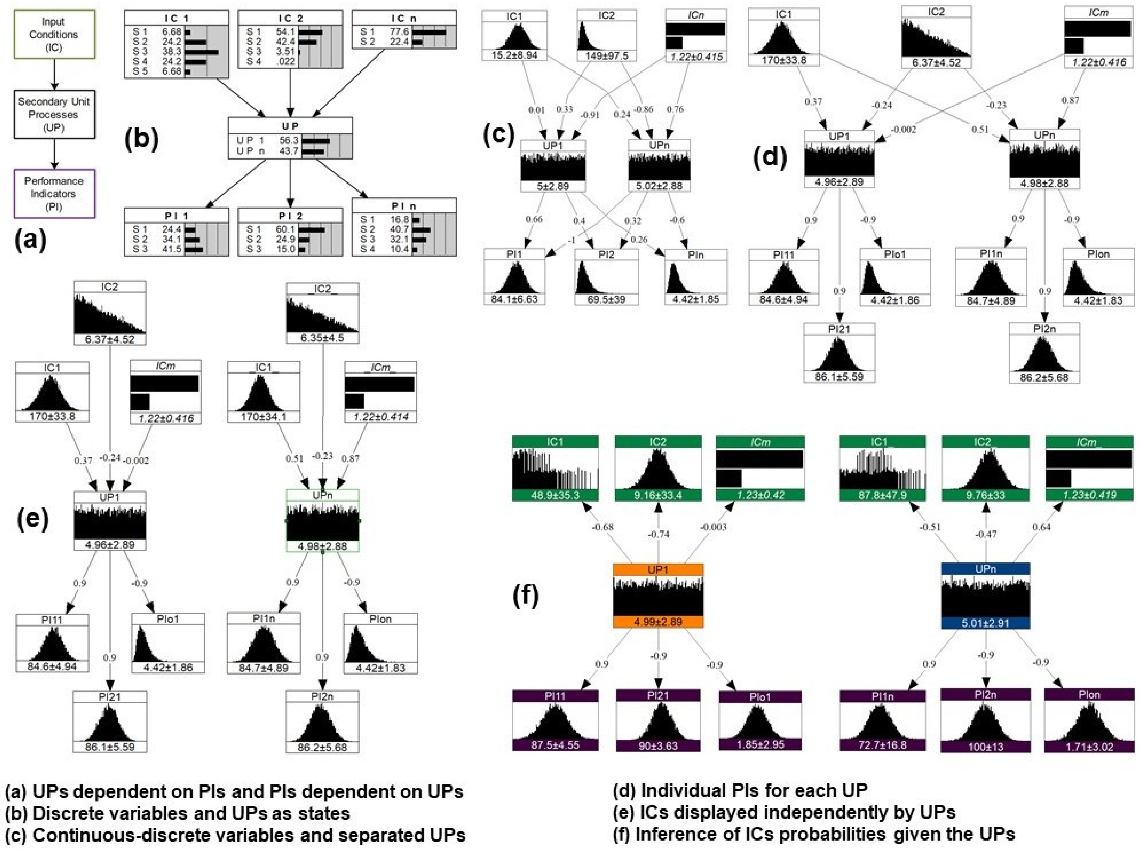
The Bayesian network can work without arcs between the ICs, UPs and PIs themselves, as well as arcs from ICs to PIs, allowing only UPs dependent on PIs and PIs dependent on UPs (Figure 2a). In this way, different potential configurations of the Bayesian network can be conceived considering discrete variables and UPs as states (Figure 2b), continuous-discrete variables and separated UPs in continuous variables (Figure 2c), individual PIs for each UP (Figure 2d), ICs displayed independently by UPs (Figure 2e): and inference of ICs probabilities given the UPs (Figure 2f).

Marginal PDFs and range correlations (stage 3) associated with the most appropriate Bayesian network of the model can be estimated from information found in databases; however, structured expert judgements can become an alternative source of data, especially to support uncertainty analysis [45].

For marginal PDFs of UPs to be defined as continuous variables, a score can be assigned to them, useful for decision making, in a range of 0 to 10 (uniform density function).

The PDFs associated with the BOM variable (

Table 4. Procedure for determining the marginal distributions of the IC and their rank correlations with the UP. Normal distributions are assumed except for the transformed ones.

IC	UP Related to IC	Source of Data	Mean and SD of PDF	Mean and SD of Marginal PDF by UP	Optimal Value (Median)	Mean and SD of Transformed Marginal PDF	Mean and SD of Transformed PDF	CP	R
{1}	{2}	{3}	{4}	{5}	{6}	{7}	{8}	{9}	{10}
BOM	RBC (1)	[33,36,47]	235.70 ± 37.10	200.50 ± 53.50	235.70	MMDOM1 ± SMDOM1	MMDO1 ± SMDO1	PMDO1	RMDO1
	TRF (2)		119.80 ± 86.50		119.80	MMDOM2 ± SMDOM2	MMDO2 ± SMDO2	PMDO2	RMDO2
	AEL (3)		225.00 ± 31.50		225.00	MMDOM3 ± SMDOM3	MMDO3 ± SMDO3	PMDO3	RMDO3
	ASL (4)		241.90 ± 41.50		241.90	MMDOM4 ± SMDOM4	MMDO4 ± SMDO4	PMDO4	RMDO4
TMP	RBC (1)	Experts Judgement	MTMP1 ± STMP1	MTMPM ± STMPM	OTMP1	MTDOM1 ± STDOM1	MTDO1 ± STDO1	PTDO1	RTDO1
	TRF (2)		MTMP2 ± STMP2		OTMP2	MTDOM2 ± STDOM2	MTDO2 ± STDO2	PTDO2	RTDO2
	AEL (3)		MTMP3 ± STMP3		OTMP3	MTDOM3 ± STDOM3	MTDO3 ± STDO3	PTDO3	RTDO3
	ASL (4)		MTMP4 ± STMP4		OTMP4	MTDOM4 ± STDOM4	MTDO4 ± STDO4	PTDO4	RTDO4
WWF	RBC (1)	[48]	3.81 ± 7.23	9.16 ± 33.14	Not applies	Not applies	Not applies	0.22	−0.74
	TRF (2)		5.52 ± 8.62					0.32	−0.47
	AEL (3)		2.81 ± 12.70					0.31	−0.54
	ASL (4)		24.89 ± 63.86					0.65	0.41
CLS	RBC (1)	[49] and Experts Judgement	Not applies	p(state 1) = 0.78	Not applies	Not applies	Not applies	PCLS1	RCLS1
	TRF (2)							PCLS2	RCLS2
	AEL (3)			p(state 2) = 0.22				PCLS3	RCLS3
	ASL (4)							PCLS4	RCLS4

SD: standard deviation; CP: conditional probability; R: rank correlation.

, column 4) can be obtained by means of the reported efficiencies (column 3) in relation to some regulations, such as the Mexican one (30 mg/L BOD₅) [46]. For example, the average reported efficiency of an RBC is 82.5% and the maximum 92.5%, so it is appropriate to manage BOD₅ concentrations in the range of 171.4 to 400 mg/L (or 300 mg/L, considering the concentration limit in municipal wastewater). In the case of TMP, these data are obtained through expert judgement.

As normal distributions, synthetic random samples are generated [25,50] to obtain the parameters of the marginal PDFs (Table 4, column 5) with the set of four samples of each variable.

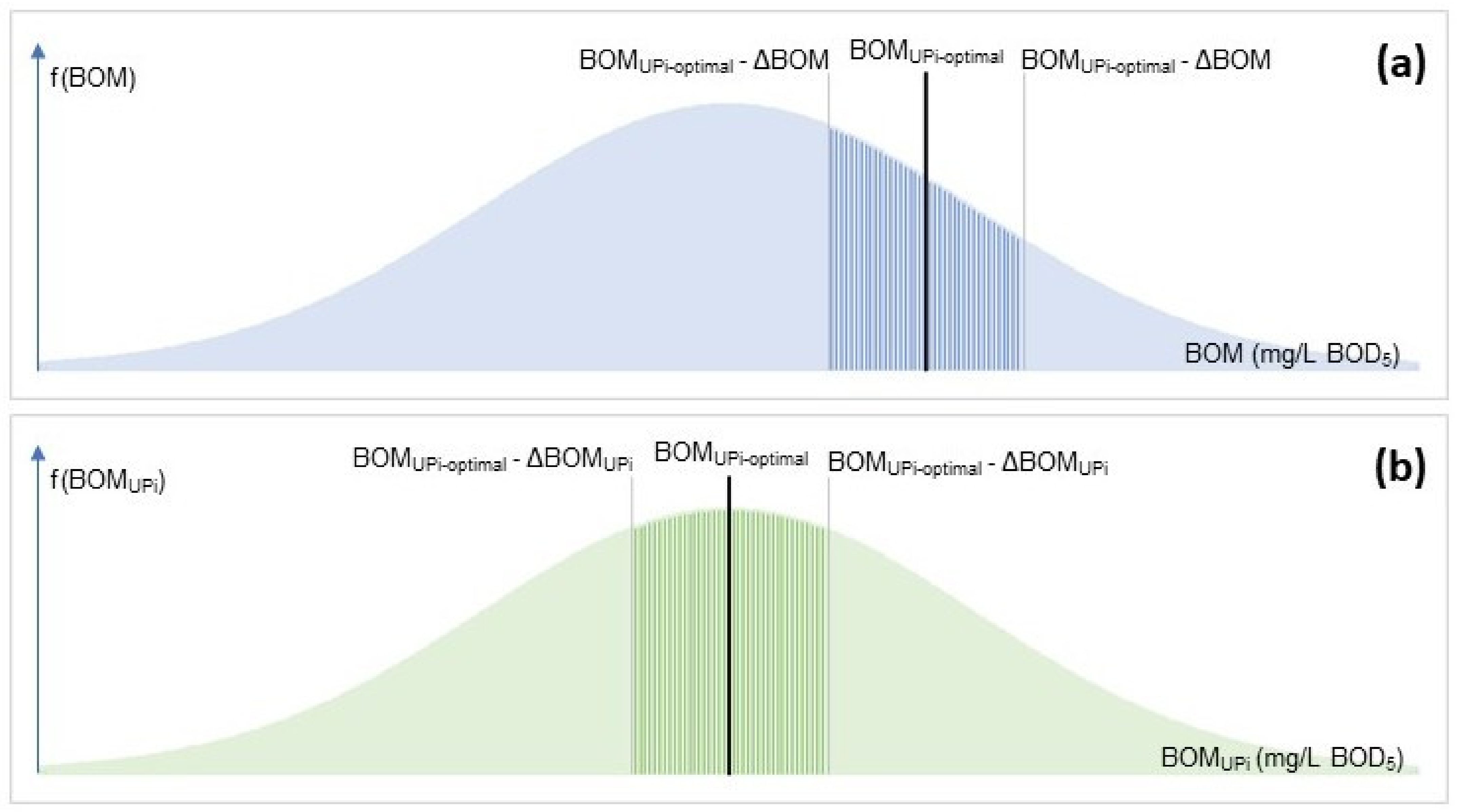
The above conception of BOM and TMP variables, although correct, is incomplete because it can lead to inconsistencies for the model. That is, the high range correlations (r > 0.8) obtained between the BOM or TMP with each UP can underestimate the other variables. To solve this inconsistency, the BOM variable can be conceived as the “biodegradable organic matter difference with the optimal one for each process” (MDO). The optimal biodegradable O. M. is the median of each process, assuming that moving away from it implies that the process decreases its probability of treating that O. M., and another process increases its probability of treating it. Therefore, the term “optimal” does not refer to the best performance of the process, but to the maximum eligibility of the process. In the case of TMP, the performance of a process does not depend on its operation at a high or low temperature of wastewater, but on how much its average operating temperature moves away from the optimal operating temperature of each process. Therefore, the TMP variable can be adjusted as “difference in wastewater temperature with optimal process operating temperature”, which is hereinafter referred to as “temperature difference with optimal” (TDO).

Examining the meanings of the optimal values, it follows that they are in the center of the PDFs of each UP (Table 4, column 6), providing four transformed marginal PDFs (column 7). The optimal value of each UP (e.g., BOM_UPi-optimal) is located in the marginal (original) distribution of MOB or TMP (Figure 3a). Therefore, the probability of having a difference (e.g., biodegradable O. M.), or lower, with the optimal value, are the cumulative probabilities on both the left and right. In this way, a cumulative probability distribution is defined based on different increments of the variables.

Similarly, the transformed PDFs of each UP (Table 4, column 8) are obtained by means of the optimal values (Figure 3b), which correspond to the median of the PDFs. The new distributions of each UP are useful for estimating the range correlations between the MDO and TDO variables with their respective UP.

CONAGUA (National Water Commission) [48] provides the implemented processes and design flows (installed capacity) of each plant registered in Mexico. Assuming a normal distribution of values, with the PDFs of WWF estimated of each UP (Table 4, column 4), a synthetic random sample is constructed per process, and, with the four joint synthetic samples, the marginal PDF is obtained (column 5).

Due to the lack of data that allow us to correlate the ICs with the proposed score for the UP, in this study, it is proposed to obtain the range correlations of the variables MDO, TDO and WWF with the UPs by conditional probabilities [51] but replacing the probabilities given by the experts with probabilities obtained through PDFs of each process and the medians of the marginal PDFs. For example, to determine the correlation between the WWF variable and the TRF variable, it must be obtained from the experts: the probability that the WWF is greater than 9.2 m³/d if the TRF score is greater than 5.0. Assuming that a score greater than 5.0 results in the process being tempted and chances of being chosen, a judgement may now be required of the experts: the probability that the WWF is greater than 9.2 m³/d if TRF is eligible. The fact that TRF is eligible means that, there are flow rates that it can handle. Additionally, these flows, defined by the PDF, can be taken into account to determine the probability. Therefore, with the marginal distribution of WWF (Figure 4a; Table 4, column 5) the median is located, and with the flow rates distribution of TRF (WWF_TRF; column4) is calculated the probability of surplus (conditional probability, column 9), to calculate the range correlation (column 10) using the method described by Morales et al. [51].

Finally, similar to the WWF variable, from the median given by the cumulative marginal PDF of MDO (or TDO) associated with an UP (F_marginal(MDO_UPi)) (Figure 4b; Table 4, column 7) and with the cumulative PDF of the MDO of the same process (F(MDO_UPi)) (column 8), the probability of surplus (column 9) required to determine the range correlation (column 10) between MDO_UPi and UPi is calculated.

Some variables, such as CLS, can be defined as a continuous–discrete variable with two states, in this case including processes that can be close to populations (up to 200 m) and those that must be away from them (at more than 1000 m) [52]. It can be assumed that in a rural town, where the population centers are distant, land is available far enough from the population to opt for any process without undesirable effects on society. In the case of an urban population, it is likely that only land close to the population is available, and processes that have fewer undesirable effects should be opted for. Therefore, it is assumed that the probability of building a plant at less than 1000 m (near, state 1) is equal to the probability of having an urban population, and the probability of building it at more than 1000 m (away, state 2) is equal to the probability of existence of a rural population. For example, in Mexico 77.6% of the population is urban and 22.4% of the population is rural [49], percentages that can define the probability distribution of the CLS variable (Table 4, column 5). Range correlations (column 10) are calculated directly from the conditional probabilities (column 9) provided by experts, for example, the probability of placing the plant at 1000 m away if AEL is chosen.

The marginal distributions of the OMR, SSR and SLD variables dependent on each of the UPs can be determined with the interval values reported in the literature, e.g., the removal efficiency of O. M. in terms of BOD₅ from a trickling filter is between 45% and 81% [36,47]. Marginal PDFs resulting from each variable and process are proposed to estimate with synthetic samples based on information provided by Asano et al. [5], César-Valdez & Vázquez-González [33], Adams et al. [36] and Wang et al. [47]

As for STY, three classes can be distinguished depending on the biological process. The lagoons are a very stable process due to the volume of the reactor, as even the same lagoon is considered as the regulation of the treatment plant [47]. Trickling filters can be considered stable because they have no significant variations in O. M. removal efficiencies, even with fluctuations in hydraulic and organic wastewater loads [53,54]. Activated sludge is an unstable process because it requires the control of variables such as feed/biomass ratio, hydraulic retention time, and amount of aeration, and it is susceptible to bulking (elevation of sludge volume in secondary settler) [47]. With these considerations, it can be established that AELs have stability 3; CBRs and TRFs, stability 2; and ASLs, stability 1. Such stability may vary depending on the process variants, but, as at this stage (research) the effects of the variants are not analyzed, these values will be constant for each process. This results in no correlation between STY and UP scoring, so they cannot be established as Bayesian network nodes, but only as variables displayed in decision support.

The CPY values of each UP can also be considered as constant values, so similar to STY, they are displayed only as a support for the decision: ASL with a complexity of 20; RBC, complexity of 11; TRF, 10; and AEL, 5 [55].

Chhipi-Shrestha et al. [2] provide approximations for estimating the construction cost, operation cost and energy consumption of different treatment processes depending on the operating flow rate. From these, unit values, relative to the flow rate, CCO, OCO and ENC of each UP (

Table 5. Total and unitary CCO, OCO and ENC of the UP, own elaboration based on [2].

Process	RBC	TRF	AEL	ASL	RBC	TRF	AEL	ASL
Flow (m3/d)	CCO (US$)				CCO (US₵/m3)
1000	0.60	0.57	0.01	0.96	8.23	7.78	0.01	13.08
4000	1.21	1.15	0.01	2.62	4.15	3.95	0.01	8.96
40,000	6.38	5.99	26.18	17.44	2.18	2.05	8.96	5.97
400,000	48.21	44.44	296.90	155.90	1.65	1.52	10.16	5.34
440,000	52.65	48.51	326.78	171.76	1.64	1.51	10.17	5.34
			Mean		1.90	1.76	9.62	5.58
			Standard deviation		2.91	3.03	5.17	1.23
Flow (m3/d)	OCO (million US$/year)				OCO (US$/m3)
1000	14.10	13.00	0.02	19.80	38.70	35.60	0.04	54.26
4000	56.50	52.00	0.04	79.20	38.69	35.58	0.03	54.25
40,000	564.70	519.40	0.23	791.80	38.68	35.57	0.02	54.24
400,000	5646.50	5192.90	1.64	7917.60	38.67	35.57	0.01	54.23
440,000	6211.10	5712.20	1.79	8709.30	38.67	35.57	0.01	54.23
			Mean		38.68	35.57	0.013	54.23
			Standard deviation		6.56	3.45	32.11	22.11
Flow (m3/d)	ENC (kWh/d)				ENC (Wh/m3)
1000	6.00	40.00	225.00	1506.00	5.92	40.29	225.00	1506.20
4000	12.00	80.00	425.00	1990.00	2.96	20.12	106.13	497.38
40,000	83.00	563.00	2819.00	7789.00	2.07	14.07	70.46	194.73
400,000	792.00	5387.00	26,759.00	65,785.00	1.98	13.47	66.90	164.46
440,000	871.00	5923.00	29,419.00	72,229.00	1.98	13.46	66.86	164.16
			Mean		2.05	13.98	69.94	190.36
			Standard deviation		67.03	55.17	15.64	178.61

) can be estimated (at increments of 4000 m³/d). These values determine the marginal PDFs of the variables for each UP.

To determine the range correlations between PIs and UPs, three statements derived from PI characteristics are taken into account:

• The higher rated (higher score) a process to treat certain wastewater is, the higher the chances of obtaining high O. M. and TSS removal increase.
• The lower graded (lower score) a process is, the higher the chances that sludge production and costs (monetary and environmental) increase.
• Because PIs are measured directly from and characterized by UP, there is a strong correlation between the UP and its PIs.

The first two statements imply the signs of range correlations, positive for removal efficiencies, and negative for sludge production and costs. As for the magnitude, a value of 0.9 is proposed, according to [56,57,58], as a strong correlation.

Although the Bayesian network integrates the main part of the model, it is necessary to define the decision mechanisms. Under this decision model, it is possible to provide two results: the score of the UP and the probability of a favorable event in the PIs determining the ICs. When a user sets values in ICs, useful probability distributions to determine the probabilities of meeting selection criteria are provided. For example, what is the most appropriate process according to ICs? (higher score), which process is most likely to exceed an O. M.? What process is most likely to be below a certain cost? In order to perform these comparisons, the scores and probabilities of getting a favorable event in a PI are displayed per process on a single web chart. This chart will allow the user to easily decide which variables have the highest weight, according to the criterion, and choose the process. In addition, it allows us to observe quantitatively and globally the advantages and disadvantages presented by the processes.

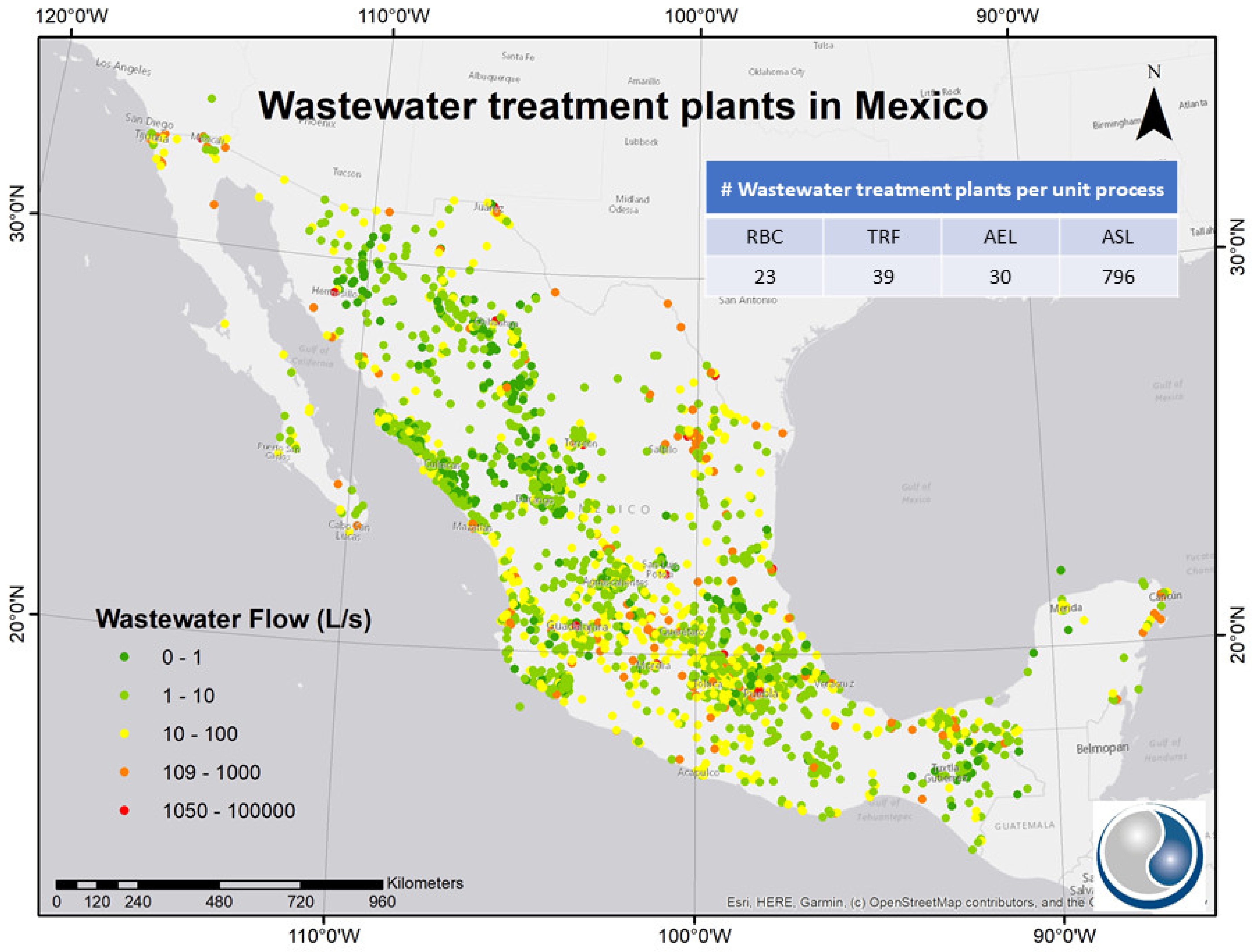
To evaluate the model, it is necessary to collect information about WWTPs (stage 4). In Mexico, CONAGUA [48] has registered 888 wastewater treatment plants (Figure 5), with the processes of this study. The database has information about the flows and the type of process that was implemented, but information about TSS, the biodegradable O. M., wastewater temperature and proximity to homes, are required. This information can be obtained through operation reports, project proposals, technical reports and local climate reports. Therefore, a necessary database for validation is built upon the complete information about 117 treatment plants.

The performance of a statistical prediction model (stage 5) can be evaluated by measuring the correspondence or agreement between predicted and observed values [59], condensed into an array of hits and errors [60,61]. Valuations provide a number of parameters to measure model performance and a ROC chart that allows to visualize its performance [61].

The user can determine the relevance between the PIs and the score of the UPs to make their choice. In the case of validation, rules are proposed to simulate reality and eliminate the triviality of the set of model choices [61]. In this way, only the score of the UP, OMR, SLD, CCO, OCO and ENC are used for validation. Moreover, because in reality only one unit process is chosen for the project, it is determined that the process that on the radial chart had three or more criteria in its favor was chosen. If three processes are tied with two criteria, the chosen one must be the process with the highest score, since this criterion is derived from the ICs.

In addition to the results of the Bayesian network, the model must be supported under three important conditions. If the amount of TSS is less than 25 mg/L and biodegradable O. M. is less than 50 mg/L BOD₅ in the secondary treatment influent, it is recommended to increase the efficiency of the primary settler to meet the limit of the regulations (40 mg/L TSS, 30 mg/L BOD₅) [46] without a secondary treatment. On the contrary, if the 275 mg/L TSS and 300 mg/L BOD₅ are exceeded, a process for high concentrations should be chosen: ASL. The third condition is based on wastewater flow. AEL and RBC typically handle lower flow rates than TRFs, and TRFs in turn handle flows lower than ASL, so above the TRF limit (1600 L/s, maximum found in the CONAGUA [48] database), only ASL can be chosen.

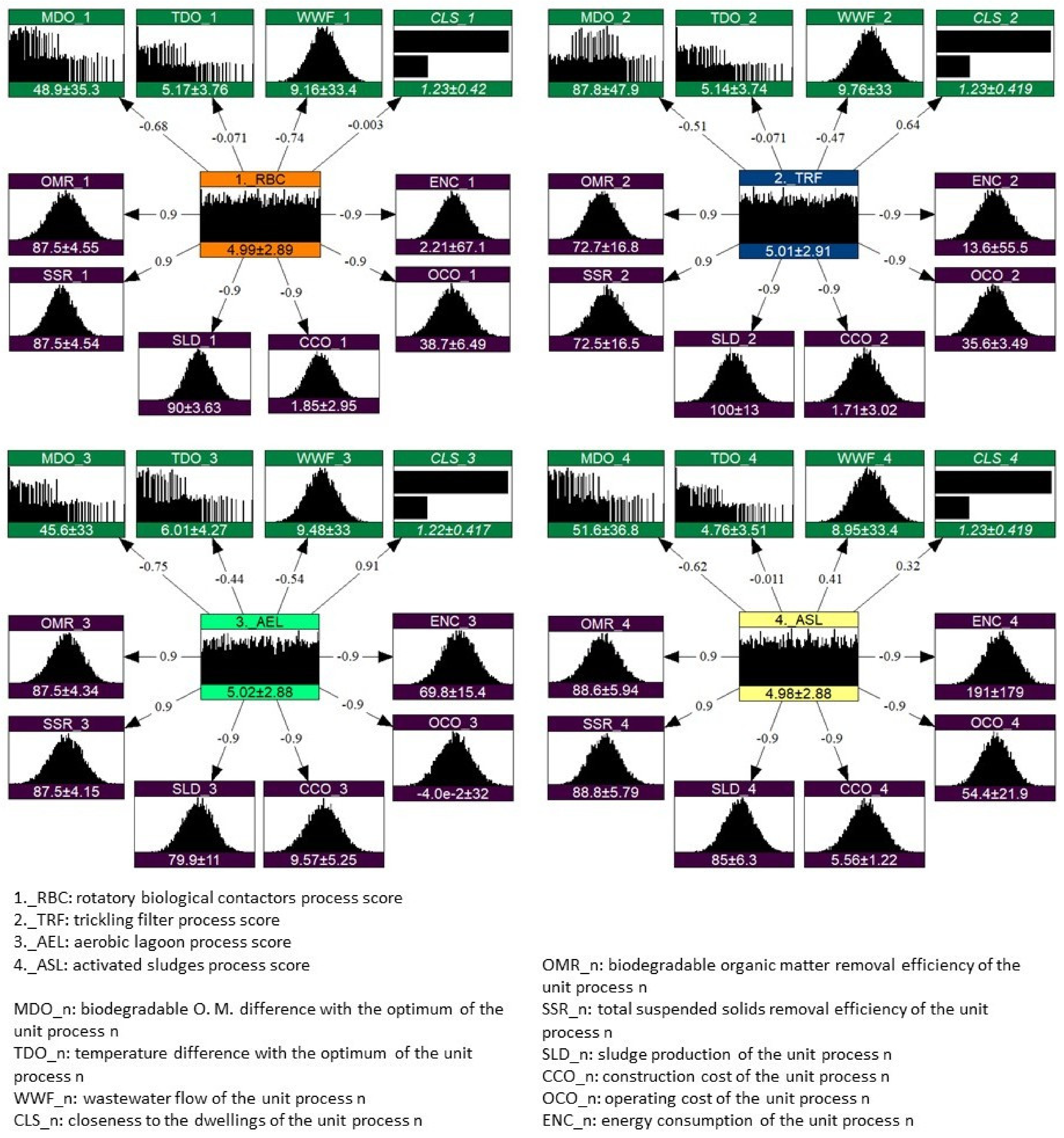
3. Results

According to the observed arguments in stage 2 of the methodology, the configuration of the selected Bayesian network was the one corresponding to the separated UPs with their own variables (i.e., UP exclusionary) with the direction of the influences (arcs) of the UPs towards the ICs (Figure 6). Although the direction of relationships in this configuration could be considered non-causal, from a mathematical or abstract point of view, Bayesian networks do not impose the direction of the causal arc [62]. In this configuration the MDO and TDO variables have a different marginal distribution in the Bayesian network of each process; WWF and CLS have a single duplicate marginal in each process; and each process has its own PIs and its marginals.

For the rest of the possible configurations (Figure 2) it can be mentioned that discrete Bayesian networks (Figure 2b) allow consideration of the exclusionary nature of UPs; however, the other variables (ICs and PIs) are continuous, the accuracy of which would mean excessive network complexity, making its modeling costly [63]. This study applied continuous-discrete non-parametric Bayesian (NPBN) networks, whose configuration is reduced to the quantification of a marginal distribution per variable and to one (conditional) dependency parameter per arc [35].

The discrete nature of UPs could be treated in an NPBN, defining them in separate variables (Figure 2c). Nevertheless, the results and demands (PIs) of each UP are also excluding; hence, they are derived from a single process. Thus, each process has PIs associated with the same parameters, but in different variables (Figure 2d).

This could be considered as the most appropriate configuration, but there can be “indirect” dependency between UPs when connected by an IC, which is not consistent with the selection process. Although this is solved by properly configuring the rank correlation matrix, or, when instantiating ICs, because communication between UP is closed [41], it is preferable to represent the phenomenon with UPs that depend on their own ICs (Figure 2e).

The fourth configuration suggested complete independence between UPs but required obtaining range correlations of up to three conditions (

Table 6. Rank correlation sorts of two Bayesian network configurations.

UP Dependent on IC		ICs Dependent on UP		Available Data
{A}		{B}		{C}
Rank correlation	Correlation sort	Rank correlation	Correlation sort	Correlated variables	Obtained objective
				UPi, TSS	Cal. in E. J.
r UPi,MDO	Unconditional	r UPi,MDO	Unconditional	UPi, MDO	Cal. in E. J. and r UPi,MDO
r UPi,TDO|MDO	Conditional	r UPi,TDO	Unconditional
r UPi,WWF|MDO,TDO	Conditional	r UPi,WWF	Unconditional	UPi, WWF	Cal. in E. J. and r UPi,WWF
r UPi,CLS|MDO,TDO,WWF	Conditional	r UPi,CLS	Unconditional

r _UPi,MDO: Rank correlation of UPi and MDO; r _UPi,TDO|_MDO: Rank correlation of UPi and TDO given MDO; r _UPi,WWF|_MDO,TDO: Rank correlation of UPi and WWF given MDO and TDO; r _UPi,CLS|_MDO,TDO,WWF: Rank correlation of UPi and CLS given MDO, TDO and WWF; r _UPi,TDO: Rank correlation of UPi and TDO; r _UPi,WWF: Rank correlation of UPi and WWF; r _UPi,CLS: Rank correlation of UPi and CLS; Cal. in E. J.: calibration in experts judgment.

, column A), which generated inconsistencies such as the overvaluation of some ICs when determined by expert judgement. The Bayesian network, whose arcs are directed from the PIs to the ICs (Figure 2f), is required to calculate only unconditional correlations (Table 6, column B). On one hand, from the literature data on the TSS, MDO, and WWF variables in relation to UPs (Table 6, column C), two rank correlations were obtained (r _UPi,MDO, r _UPi,WWF). On the other hand, a structured expert judgment was carried out to obtain PDFs and remaining rank correlations from stage 3 (

Table 7. Resolution of the marginal distributions of the IC and their rank correlations with the UP.

IC	UP Related to IC	Source of Data	Mean and SD of PDF	Mean and SD of Marginal PDF by UP	Optimal Value (Median)	Mean and SD of Transformed Marginal PDF	Mean and SD of Transformed PDF	CP	R
{1}	{2}	{3}	{4}	{5}	{6}	{7}	{8}	{9}	{10}
BOM	RBC (1)	[33,36,47]	235.70 ± 37.10	200.50 ± 53.50	235.7	49.60 ± 36.60	29.90 ± 22.40	0.26	−0.68
	TRF (2)		119.80 ± 86.50		119.8	88.20 ± 49.00	68.50 ± 50.60	0.32	−0.51
	AEL (3)		225.00 ± 31.50		225.0	45.70 ± 34.20	25.40 ± 19.00	0.22	−0.75
	ASL (4)		241.90 ± 41.50		241.9	52.40 ± 38.20	33.40 ± 25.00	0.28	−0.62
TMP	RBC (1)	Experts Judgement	22.50 ± 6.150	24.80 ± 6.05	22.5	5.20 ± 3.89	4.90 ± 3.70	0.48	−0.07
	TRF (2)		22.50 ± 6.15		22.5	5.20 ± 3.89	4.93 ± 3.70	0.48	−0.07
	AEL (3)		29.30 ± 5.65		29.3	6.12 ± 4.41	4.53 ± 3.40	0.35	−0.44
	ASL (4)		25.00 ± 6.00		25.0	4.85 ± 3.65	4.81 ± 3.61	0.50	−0.01
WWF	RBC (1)	[48]	3.81 ± 7.23	9.16 ± 33.14	Not applies	Not applies	Not applies	0.22	−0.74
	TRF (2)		5.52 ± 8.62					0.32	−0.47
	AEL (3)		2.81 ± 12.70					0.31	−0.54
	ASL (4)		24.89 ± 63.86					0.65	0.41
CLS	RBC (1)	[49] and Experts Judgement	Not applies	p (state 1) = 0.776	Not applies	Not applies	Not applies	0.50	−0.01
	TRF (2)							0.73	0.64
	AEL (3)			p (state 2) = 0.224				0.87	0.91
	ASL (4)							0.61	0.32

SD: standard deviation; CP: conditional probability; R: rank correlation.

).

In this expert judgement, the values obtained for the temperature variable in RBC and TRF are equal, as it is expected. From Table 2, these two processes show the same operation level with respect to temperature, i.e., both processes work with the same type of microorganisms, attached biofilm and have natural (not forced) aeration. Therefore, their appropriate operating temperatures must be similar.

A reliable expert judgment requires calibration questions to assess the performance of the experts and give them a weight in the combination of their opinions (decision maker). Therefore, a questionnaire involving all the ICs was elaborated to determine the marginal distributions of the TDO variable and the rank correlations of the CLS variable with the UPs. The variables TSS, BOM and WWF depicted the calibration questions (see Appendix A,

Table A1. Data obtained from experts for the determination of marginal PDFs of the TDO variable and range correlations of UP and CLS.

IC	UP	ID	Expert												R
			1			2			3			4
			Quantile (%)
			5	50	95	5	50	95	5	50	95	5	50	95
TSS	CBR	6.1	175	212.5	250	250	325	400	50	250	450	100	225	350	381
	FPR	7.1	200	250	300	200	275	350	50	125	200	100	150	200	160
	LAE	8.1	800	1150	1500	250	325	400	100	300	500	100	300	500	500
	LAS	9.1	700	850	1000	300	400	500	100	275	450	100	300	500	458
BOM	CBR	6.2	100	125	150	300	500	700	100	275	450	100	225	350	286
	FPR	7.2	80	100	120	400	575	750	50	150	250	100	225	350	120
	LAE	8.2	500	700	900	500	625	750	100	275	450	100	300	500	375
	LAS	9.2	300	500	700	400	550	700	150	325	500	100	300	500	344
TDO	CBR	6.3	15	20	25	10	15	20	10	22.5	35	5	22.5	40	E
	FPR	7.3	15	20	25	10	12.5	15	10	22.5	35	5	22.5	40	E
	LAE	8.3	12	20	28	15	20	25	18	26.5	35	25	32.5	40	E
	LAS	9.3	15	21.5	28	15	20	25	5	25	45	10	25	40	E
WWF	CBR	6.4	60,000	90,000	120,000	40	50	60	20	5010	10,000	50	225	400	3812
	FPR	7.4	100,000	150,000	200,000	60	70	80	20	10,010	20,000	400	1200	2000	5523
	LAE	8.4	40,000	60,000	80,000	40	50	60	20	1010	2000	20	1010	2000	2809
	LAS	9.4	100,000	150,000	200,000	40	50	60	20,000	110,000	200,000	2000	51,000	100,000	9267
CLS	CBR	6.5	5	7.5	10	1	1.5	2	40	60	80	10	50	90	E
	FPR	7.5	5	12.5	20	1	1.5	2	5	12.5	20	10	30	50	E
	LAE	8.5	20	35	50	1	1.5	2	10	17.5	25	1	10.5	20	E
	LAS	9.5	70	80	90	1	1.5	2	30	50	70	10	30	50	E

Combining each IC with a UP (IC, UP): IC values that can successfully handle by a PU in the quantiles (5, 50, and 95%). For example, (TSS, TRF): The amount of TSS that TRF can properly treat in those quantiles. R: realization, the actual value of the calibration question; E: Information sought from the experts; ID: The ID of the question.

).

From the data of the structured expert judgment treated with the Excalibur v1.0 program [64], the weight of the results was determined: expert 3, 30.69%; and expert 4, 69.31% (

Table A2. Expert calibration and information.

Expert	1	2	3	4	DM
Calibration score	0.000002	0.000001	0.061	0.124	0.228
Information score	1.026	2.231	0.822	0.909	0.779
Weigh	0.001	0.002	30.690	69.310

DM: Decision maker.

). Such results, where one or two experts get all the weight of the DM are not erroneous or atypical results [65], as in the Colson and Cooke [66] study, where two experts out of nine take virtually all the weight of the information. According to [65], each expert can access different information or can interpret it differently, so there is no logical reason why all experts must have the same state of knowledge.

DM reliability (22.82%; calibration score) resulted above the recommended limit (5%) [67], and the DM information score (0.7786) was only three times less than the greatest score provided by expert 2 (2.309). Due to the proper calibration score and admissible information score obtained, it was not necessary to interview more experts to get the necessary values (

Table 8. Values obtained from expert judgment.

IC	UP	Quantile (%)			Normal Distribution Parameters
		5	50	95	Mean	Standard Deviation
Temperature (°C)	RBC	5.46	22.50	39.54	22.50	5.68
	TRF	5.46	22.50	39.54	22.50	5.68
	AEL	18.83	30.81	39.77	29.30	3.49
	ASL	6.79	25.00	43.21	25.00	6.07
IC	UP	Quantile (%)			p (CLS < 1000)	p (CLS > 1000)
CLS	RBC	11.18	54.70	89.06	0.50	0.50
	TRF	5.60	21.11	49.18	0.27	0.73
	AEL	1.29	13.02	24.74	0.13	0.87
	ASL	10.51	36.14	68.14	0.39	0.61

). This means that experts 3 and 4 are highly informative and provide the required data.

With the model developed and the database generated (stage 4), the selection of the treatment was carried out by the plant. For example,

Table 9. Input data examples of some cases for the model.

	Characteristic or Parameter	Unit	Plant (#)
			001	002	010	098
Case of study	Implemented process		ASL	ASL	TRF	ASL
	Total suspended solids	(mg/L TSS)	376.01	32.00	184.60	261.00
	Biodegradable O. M.	(mg/L BOD5)	393.54	55.90	369.00	334.00
	WW temperature	(°C)	23.64	19.45	23.20	27.72
	Wastewater flow	(L/s)	100.00	200.00	237.50	171.00
	Closeness to homes		close	close	close	close
Bayesian network	MDO RBC	(mg/L BOD5)	29.94 *	197.97	13.38	10.25
	MDO TRF		145.84	82.07	129.28	105.65
	MDO AEL		40.64	187.27	24.08	0.45
	MDO ASL		23.74 *	204.17	7.18	16.45
	TDO RBC	(°C)	1.14	3.06	0.70	5.22
	TDO TRF		1.14	3.06	0.70	5.22
	TDO AEL		5.66	9.86	6.10	1.58
	TDO ASL		1.36	5.56	1.80	2.72
	WWF	(m3/d) * 1000	8.64 *	17.28	20.52	14.77
	CLS	(state)	1	1	1	1
Process chosen by the model			ASL	TRF	ASL	AEL

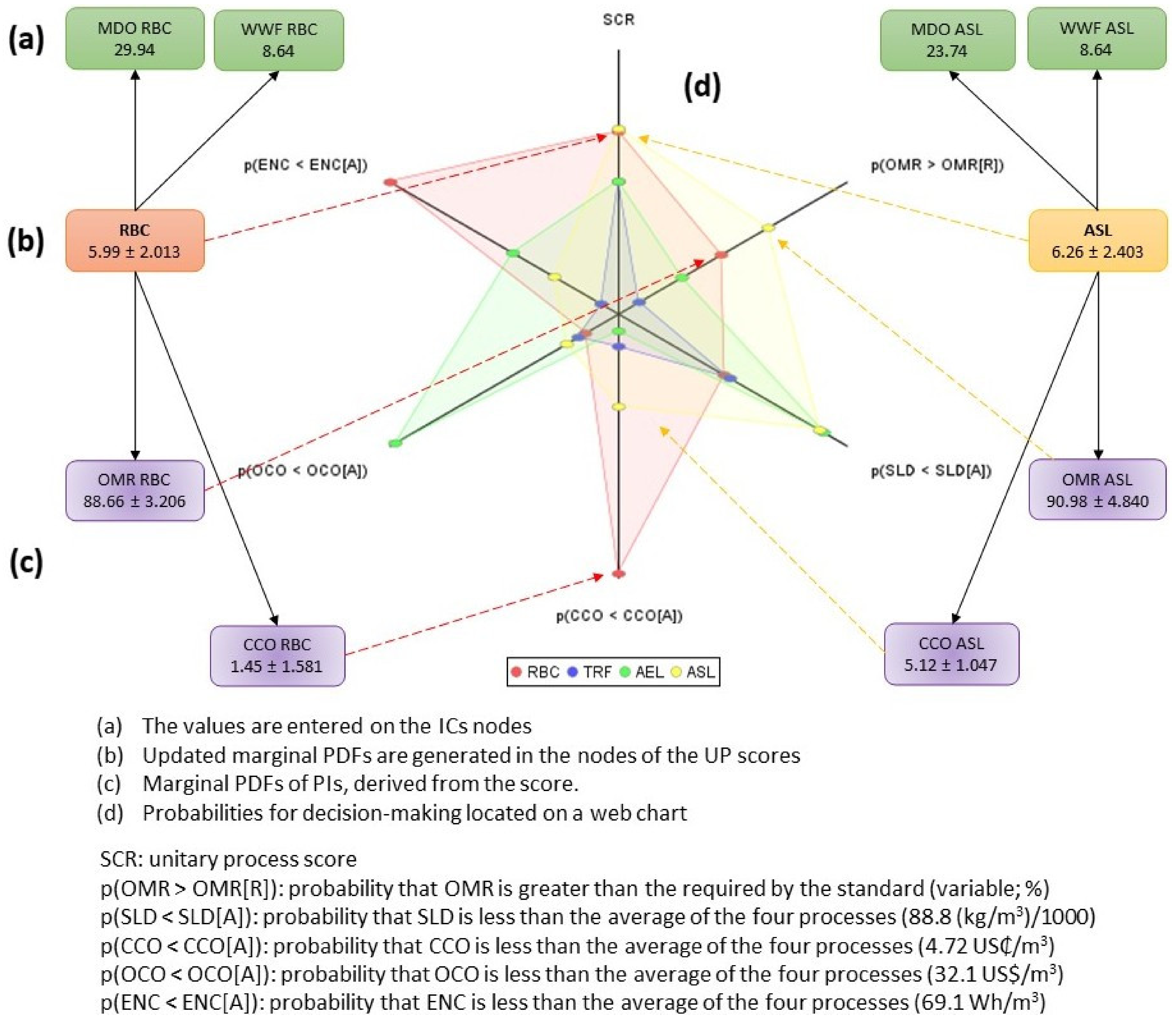
* Values used in the example in Figure 7.

shows data from four strategic WWTPs: one with successful selection, one with incorrect selection, and two belong to a group of 40 plants in the database whose type of processing was assumed to be the least appropriate. Four MDO and TDO values can be seen because these are obtained in return to the optimal value of each process, and only one for WWF and CLS value.

The values were entered on the ICs nodes (Figure 7a), and as a result updated marginal PDFs were generated in the nodes of the UP scores (Figure 7b). In the example, it is observed that ASL is the most appropriate process, by the average scoring values, which are derived from the ICs. This result already represents a trend in the decision, but it is desirable to assess PIs to strengthen the selection. With marginal PDFs of PIs derived from the score (Figure 7c), it was possible to determine useful probabilities for decision-making, e.g., the probability of exceeding, with one process, the O. M. removal efficiency required to comply with a standard (or a proposed efficiency value) or the probability of having, with the process, a lower cost than the average of the four processes (or a required cost). To assist in comparing the four scores and the four probabilities obtained from each PI, it was proposed to place the values on a web chart (Figure 7d) that shows which processes are most favored according to PIs.

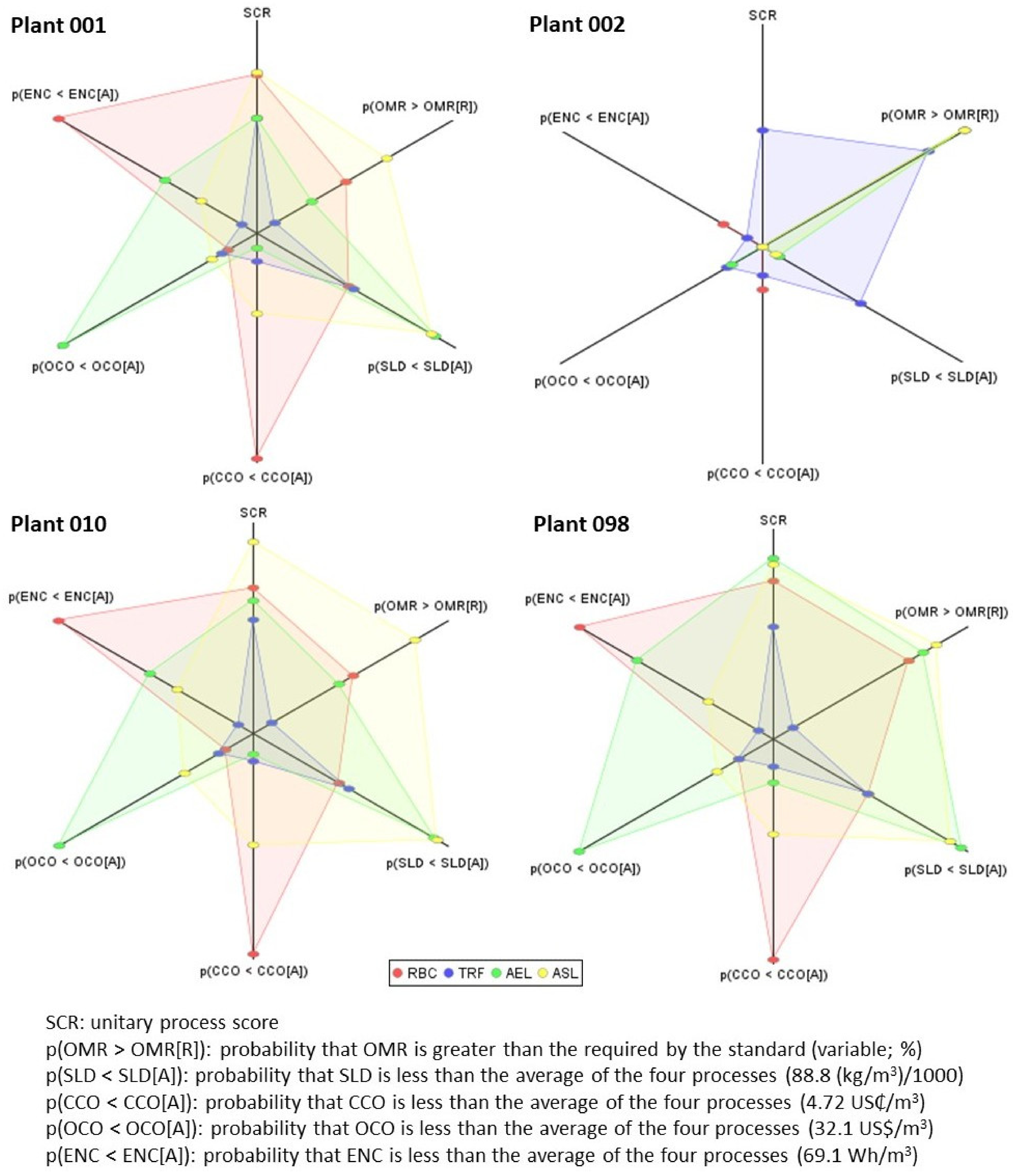
For stage 5, all 117 case studies were rated. However, as a comparison, in the case of Plant 001, it can be observed that the process chosen by score (Figure 8) matches that implemented (ASL) and shows three processes with two favorable indicators. The choice of model and case will be corroborated when analyzing the input values: high values of biodegradable O. M., a temperature close to the optimal of ASL and location close to the population. Perhaps the only inconvenience to choose ASL is a relatively low flow, so RBC is approaching similar values in scoring and could be contemplated.

The input data for Plant 002 (from Table 9) indicate that the process to be chosen was a TRF, as suggested by the model (it has three PIs in its favor; Figure 8). The values of biodegradable O. M. are so low that they support the decision to choose TRF, and the temperature of the WW approaches its optimal value (22.5 °C) and there is a favorable flow for the process. Therefore, because an ASL was implemented, this case, along with similar ones, are considered to have an unsuitable process.

An opposite case is observed at the Plant 010 where a TRF is implemented, and the model chooses ASL. It is observed that the biodegradable O. M. that enters has a very high concentration for a TRF. Although, it is possible to treat these concentrations with the implemented process, it is necessary to raise the costs of construction and operation, which leads to analyzing a balance between cost and efficiency obtained. In this way, the choice is between an expensive TRF with less chance of obtaining efficiencies or an ASL, which is also expensive, with a high chance of efficiencies. With this approach, this case study and similar ones that were found, were considered as unsuitable processes.

In the last example, the model chose AEL, but ASL was implemented. It was considered an incorrect choice because the plant is close to a population center, which can definitely eliminate this option, and also the magnitude of the flow exceeds what it (AEL) can conventionally treat. On the other hand, the tendency of the model to choose AEL is justified by having a process-friendly temperature and biodegradable O. M.: 27.7 °C with an optimal process temperature of 29.3 °C; and 225 mg/L BOD₅ in the secondary treatment influent with optimal BOM of the same value.

For validation, the valuation parameters by UP and globally were calculated (

Table 10. Successes and errors accounting of the case studies and values of the useful parameters for the validation of the model.

Parameter	RBC	TRF	AEL	ASL	Global
T+	1	6	0	59	66
F+	0	7	5	1	13
F−	0	1	0	13	14
V−	76	63	72	4	215
F+R	0.000	0.100	0.065	0.200	0.057
T+R	1.000	0.857	--	0.819	0.825
PP+	1.000	0.462	0.000	0.983	0.835
PP−	1.000	0.984	1.000	0.235	0.939
Kappa	1.000	0.546	0.000	0.293	0.771
+CP	0.013	0.091	0.000	0.935	0.260
Sensitivity	1.000	0.857	--	0.819	0.825

T+: true positives; F+: false positives; F−: false negatives; T−: true negatives; F+R: false positive rate; T+R: true positives rate; PP+: positive predictive power; PP−: negative predictive power; +CP: positive cases prevalence.

) according to the equations shown by Fielding and Bell [61].

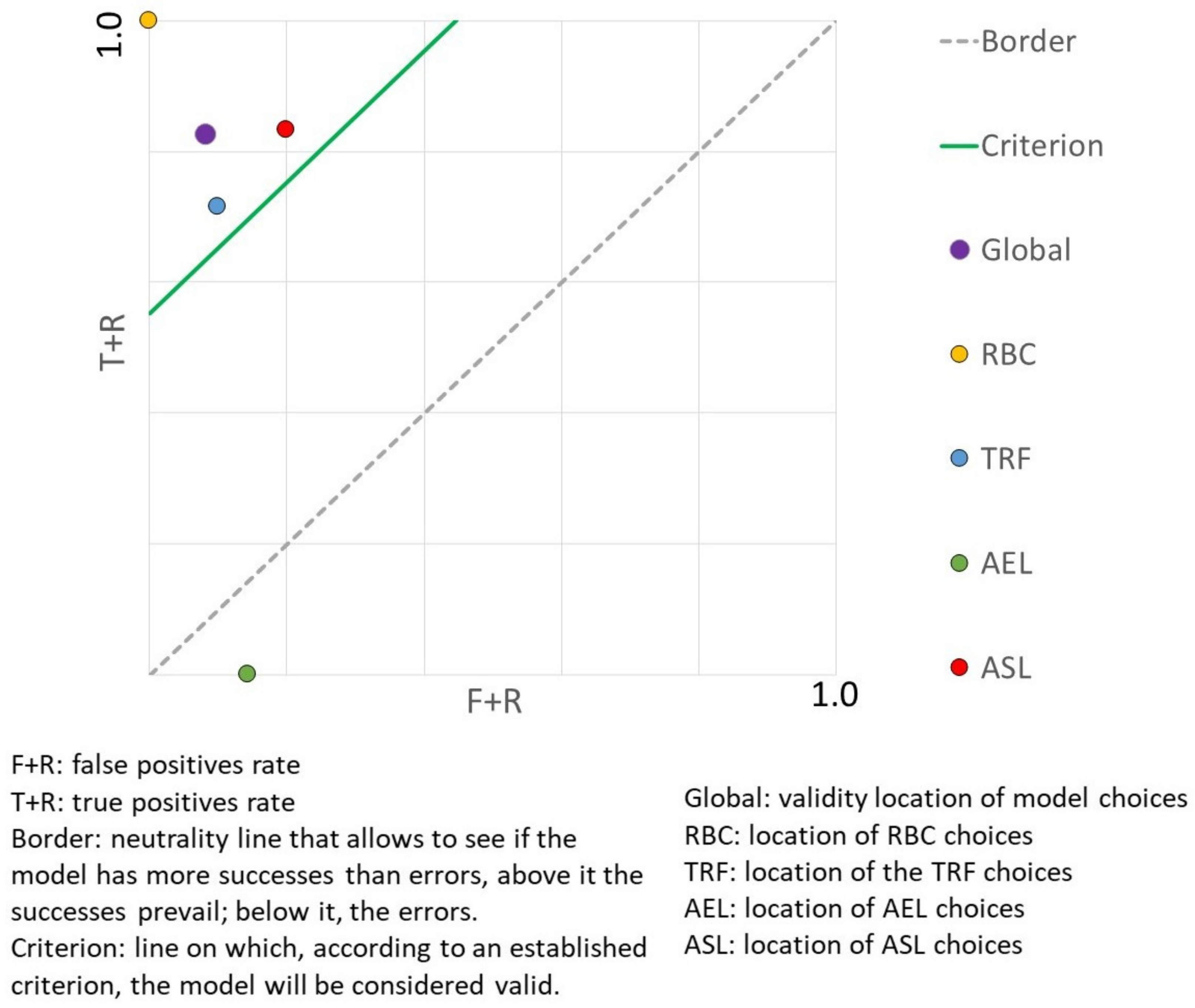
According to its location on the ROC chart (Figure 9), the model meets the established criterion (exceed 90% of the unit area); the PP+ of the model achieves a good percentage of positive predictions, 83.5%; the PP− (93.9%) influences the validation of the model to a lesser extent, since, for each case study, three processes are not observed; and, an excellent Kappa (0.77 > 0.75) is achieved [68]. UP predictions are also well positioned (above criterion) for RBC, TRF, and ASL processes (Figure 9). Only AEL predictions showed very low performance. This may be due to the fact that when choosing this process, the availability of the land for designers is decisive. Nevertheless, the model takes into account three other factors (MOB, TMP, WWF) and decides the availability of the land according to the CLS. This suggests adding a criterion to this variable, discarding the process when the plant is nearby, or giving it greater precision.

The case studies with unsuitable processes found in the database reflect a problem that exists in Mexico and probably in other regions, justifying the implementation of a methodology for choosing the wastewater treatment process. However, about 50% of the information to build the Bayesian network was obtained from American literature, so it is possible that the model can be implemented in the U.S.A. if validation is performed with data from the region. In this way, it can be generalized that the model can be useful for any region by validating it with endemic data and, if required, adjusting it with data from the region under study. One objective that is visualized is to achieve the development of a comprehensive model that can be implemented in any region, or even, achieving greater dissemination of the model, standardizing decision trends globally.

Due to the flexibility of the latest model configuration and because any process can be evaluated based on its inputs (ICs) and outputs (PIs), the model can be adjusted for other types of treatment and/or variables can be added to the Bayesian network. With the structure where the IC and PI distributions depend on the evaluation (distribution) of the UP it is possible to define a set of processes of similar type, and according to the characteristics of the set add the variables that would be involved in the decision of that set. In addition, because of that flexibility, any model could be easily improved by adding (or modifying) the necessary variables. For example, the model of this research can be improved by adding the nitrogen (or phosphorus) removal variable, for which, due to the last direction of arcs between IC and UP, it is only necessary to investigate the data of each process linked to this parameter. An unconventional treatment, such as membranes, can even be added, or process variants can be separated, requiring data according to the ICs and PIs that were defined in this study and structuring the process with their own variables.

Once the model is considered suitable for use in Mexico, or in later regions, it is important to use and broadcast the software, with an interface that takes the input data (ICs) of the design and deployment, in the proposed web graph, and the results (PIs). The Uninet software, with which the Bayesian network of this research was modeled, has a library (UninetEngine) for programming in several languages (C++, Delphi, Matlab, among others). This library requires the acquisition of a license. The Netica API is also available for discrete, free-distribution networks, for use in Java or C++, and has functions to emulate continuous variables, which are possible to use if conditional arrays are a bit complex or have dependencies on a single variable, as in the case of this investigation.

4. Conclusions

A statistical model based on Bayesian networks has been generated that underpins the choice of the optimal process of secondary municipal wastewater treatment, based on statistical data and mathematical justifications. According to the results of the validation, it provides an acceptable level of certainty based on technical, economic, social and environmental performance, so the methods carried out are supported. As this Bayesian Network-based model showed satisfactory results for aerobic wastewater treatment, it could be expanded to the selection of other types of processes, such as anaerobics or membranes, so their inclusion in later versions are suggested.

In the methodology of the model, it was important, in addition to determining the parameters associated with the variables, to define the appropriate conception of the variables and their relationship with the UPs to define the adequate marginal PDFs and range correlations, avoiding inconsistencies in the model. As for the PDFs of each process and range correlations that could not be obtained through databases, expert judgment was successfully used in obtaining this information. Some Bayesian network correlations were successfully estimated by conditional probabilities obtained from the PDFs of each process associated with the parameter of a variable and the medians of marginal PDFs associated with the same variable.

Unlike other tools for WWTPs, this model is a support mechanism prior to the design of the treatment train, which provides results based on data and the experience of experts, with no need of dimensioning the treatment train. Therefore, in addition to the known advantages, such as addressing uncertainty, an easy-to-view structure, and the evaluation of different scenarios with a single model, this model acquires significance because it provides objective and comparable information on four types of secondary treatment for a decision-making process of selection.

The criteria for choosing conventional secondary wastewater treatment were related to model variables, variable type, model type, and output type. The appropriate variable type for unit processes was the discrete variable; input variables and performance indicators could be better visualized and processed as continuous variables. The most suitable type of networks for the variables involved were continuous-discrete, non-parametric Bayesian networks, structured in different Bayesian networks by unit processes. It was useful for the choice to visualize the score value of the UP and the probabilities of meeting design demands.

Because positive predictive power and negative predictive power exceeded the required value, the Kappa parameter indicated a satisfactory valuation, and the location of validity on the ROC chart surpassed the criterion line, the model is considered valid to support the choice of secondary wastewater treatment in Mexico.

The model’s adaptability to obtaining information in an elementary way, i.e., by parameters or variables seen in isolation, allows the development methodology to be easily extended to other types of treatments of wastewater, that is, it can be used for any type of wastewater treatment plant, and also allows the model to be expanded and improved for application in other regions.