A Tailings Dam Long-Term Deformation Prediction Method Based on Empirical Mode Decomposition and LSTM Model Combined with Attention Mechanism

Abstract

Tailings dams are constructed as storage dams for ore waste, serving as industrial waste piles and for drainage. The dam is negatively affected by rainfall, infiltration lines and its own gravity, which can cause its instability to gradually increase, leading to dam deformation. To predict the irregular changes of tailings dam deformation, empirical mode decomposition (EMD) is applied to the deformation data to obtain the trend and periodic components. The attention mechanism is used to assign different weights to the input variables to overcome the limitation that the long short-term memory (LSTM) model can only generate fixed-length vectors. The lagged autocorrelation coefficient is applied to each decomposed subregion to solve the lagging effect of external factors on dam deformation. Finally, the model is used to predict deformation in multiple directions to test the generalization ability. The proposed method can effectively mitigate the problems of gradient disappearance and gradient explosion. The applied results show that, compared with the control model EMD-LSTM, the evaluation indexes RMSE and MAE improve 23.66% and 27.90%, respectively. The method also has a high prediction accuracy in the remaining directions of the tailings dam, which has a wide practical application effect and provides a new idea for tailings dam deformation mechanism research.

1. Introduction

Various types of waste are generated during mineral extraction and processing [1,2]. For example, to obtain gold and copper elements from mineral particles, the ore needs to be processed into particles of suitable size, and the remains after the extraction of gold and copper are called “tailings” [3,4]. People usually build tailings dams for tailings storage, and the risk of tailings dam failure would increase owing to factors such as internal phreatic line and external rainfall [5]. In recent years, tailings dam failures and seepage incidents have occurred frequently in the mining industry. The tailings dam itself contains hazardous substances such as leachate slag and industrial waste that can pollute farmland, rivers, and groundwater around the dam [6,7]. Once security incidents such as the tailings dam failure occur, they are prone to cause huge public events, which bring about secondary pollution to the ecological environment and huge losses to both agricultural production along the way and people’s lives and property [8]. Most of these accidents are attributed to the inability to effectively control the groundwater level in the tailings dam, resulting in groundwater seepage [9]. The free surface of the tailings dam groundwater, i.e., the groundwater level, is one of the most important factors affecting the stability of the tailings dam [10,11,12,13]. Another aspect, as the number of days increases, is that the slope displacement is significantly influenced by rainfall [14].

Effective monitoring and early warning for tailings dam deformation can reduce the risk of dam failure and minimize losses. Consequently, there is a certain necessity to establish a tailings dam deformation prediction model and provide reliably predicted values of tailings dam deformation for analyzing and assessing the stability of the tailings dam. As one of the classic methods of tailings dam deformation prediction, the multiple regression model is widely used and the input is various influencing factors. Compared with the machine-learning method, the physical interpretability is the highest, but it cannot achieve ideal accuracy in the case of a small number of parameters and a low sample size [15]. Besides, quite a few parameters in the regression model would increase the risk of overfitting and multicollinearity. In response to these problems, a space-time regression model based on centroid and the use of the partial least-squares (GA-PLS) algorithm to select variables are proposed [16,17]. The application of a regression model in dam deformation prediction is extended. Autoregressive integrated moving average (ARIMA) models from a time series perspective can achieve high accuracy in the short term [18], but have poor predictive power in the long term. A support vector machine in the machine-learning method has an ordinary prediction effect for a large sample of data [19] and is more suitable for a small sample of data. While using deep learning methods, the recurrent neural network (RNN) is prone to gradient vanishing and gradient explosion because of the network structure, and the prediction effect depends largely on the hyperparameters’ setting in the neural network model [20]. Recently, the LSTM network technology has taken full account of the length dependence in the time series, avoiding the problem of gradient vanishing and gradient explosion [21]. An LSTM network could solve the problem of RNN gradient vanishing and gradient explosion to a certain extent [22], but it still appears to be tricky when facing longer sequences and to be easy to lose sequence information while affecting the accuracy of prediction [23], and it cannot capture the importance of the input sequence as well. Compared with the ANN model, the LSTM model spends more time in training model parameters [24]. In addition, when combining the genetic algorithm with the neural network, since the genetic algorithm overcomes the problem of getting into a local minimum when finding the optimal solution, the optimized neural network model will bring a better prediction effect [25]. However, due to the complexity of the genetic algorithm model, the setting of parameters such as crossover rate and the mutation rate included in the genetic algorithm need to be determined by experience, which is not easy for generalized use. By contrast, the LSTM model, through the internal structure of the output gate, input gate and forget gate, can also avoid the problem of falling into local optimal solutions during gradient descent, compared with the genetic algorithm, which is more convenient for usage.

In recent years, with rapid development, machine learning and artificial intelligence, not only in the direction of dam deformation prediction, but also in the application of machine learning in hydrodynamics and water quality, are becoming more and more mature [26,27,28,29]. The above research fully demonstrates that machine learning has carried out a wide range of applications in the hydrogeology field and has excellent applicability.

Aimed at this problem and background, we propose the attention-mechanism-based LSTM network model in which the attention mechanism module gives different probability weights to the hidden layer of LSTM [30] Thus, this method strengthens the influence of important information, enabling it to make full use of the input variable features, taking into consideration the long-term dependence of the time series, and enhancing the attention of the prediction model to key time series [31]. Dam deformation data are affected by external factors and are featured with time sequence and nonlinearity [32]. Time sequence means that under the influence of rainfall, phreatic line and the weight of the dam itself, tailings dam deformation has a general trend of continuous decline over a long period, and the meaning of nonlinearity is that parameters in the time series data model will change over time [33]. In this study, we propose to use EMD to remove the noise of the tailings dam deformation, and the EMD-processed time series is used to predict the tailing dam deformation based on LSTM with the attention mechanism. The input is the historical data of rainfall, phreatic line and tailings dam deformation 36 moments before the prediction time. Hyperparameter tuning and model training are performed on the LSTM network and the tailings dam deformation prediction model is established. At the same time, the accuracies of EMD-LSTM, EMD-ARIMA and multiple regression models [34,35,36] are compared to verify the effectiveness of this method in the prediction of tailings dam deformation.

In Section 2, we provide the principle and deformation of the displacement process of the tailings dam, which includes a detailed method introduction. In Section 3, we describe the process of data acquisition and data preprocessing of the Zijin tailings dam (25°12′ N, 116°23′ E), including the processing of outlier and missing values. In Section 4, we describe the experimental process and result of the mixed model of tailings dam deformation prediction. Finally, in Section 5, we provide the applied result, comprehensive evaluation and future work.

2. Materials and Methods

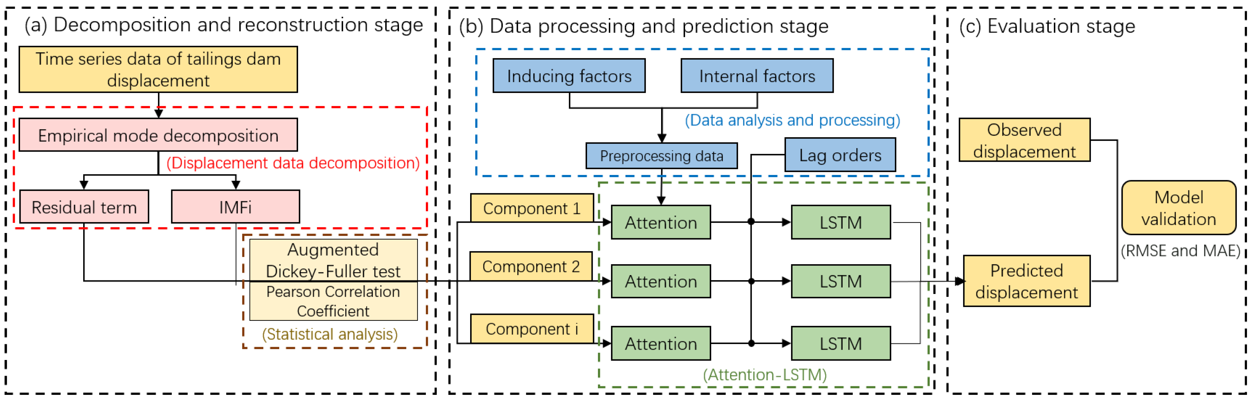
2.1. Dam Displacement Prediction Process

The flow chart of the tailings dam displacement prediction is as shown in Figure 1. The flow chart is divided into three stages: decomposition and reconstruction stage, data processing and prediction stage, and evaluation stage. These are mainly summarized as the following five contents:

(1)

Data preprocessing: elimination of outliers and missing value interpolation.

(2)

The decomposition and reconstruction of multi-factor time series data through the EMD method.

(3)

Determining the input sequence by the lag autocorrelation coefficient method.

(4)

Parameter adjustment of lagging LSTM network based on attention mechanism.

(5)

Results prediction and accuracy evaluation.

2.1.1. Principle of EMD Method

The absolute deformation in the tailings dam is nonlinear in nature. EMD is a method for processing non-stationary adaptive time-frequency data. By the EMD method, a series of intrinsic mode functions (IMFs) can be obtained from the decomposition of the signal as follows [37,38]:

$$x\left(t\right)={\displaystyle \sum }_{i=1}^{n}im{f}_i\left(t\right)+r_n\left(t\right)$$

(1)

where $im{f}_i\left(t\right)$ is the $i$th IMF obtained by EMD decomposition, and $r_n\left(t\right)$ is the residual component of the signal after sieving n IMFs from the decomposition, often representing the direct current component of the signal or its trend.

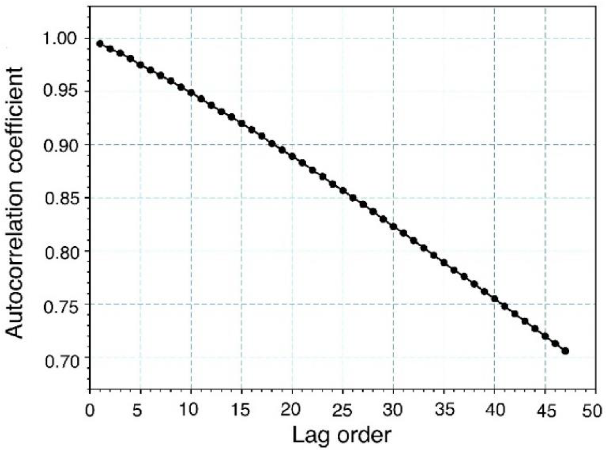
2.1.2. Lagged Autocorrelation Coefficient

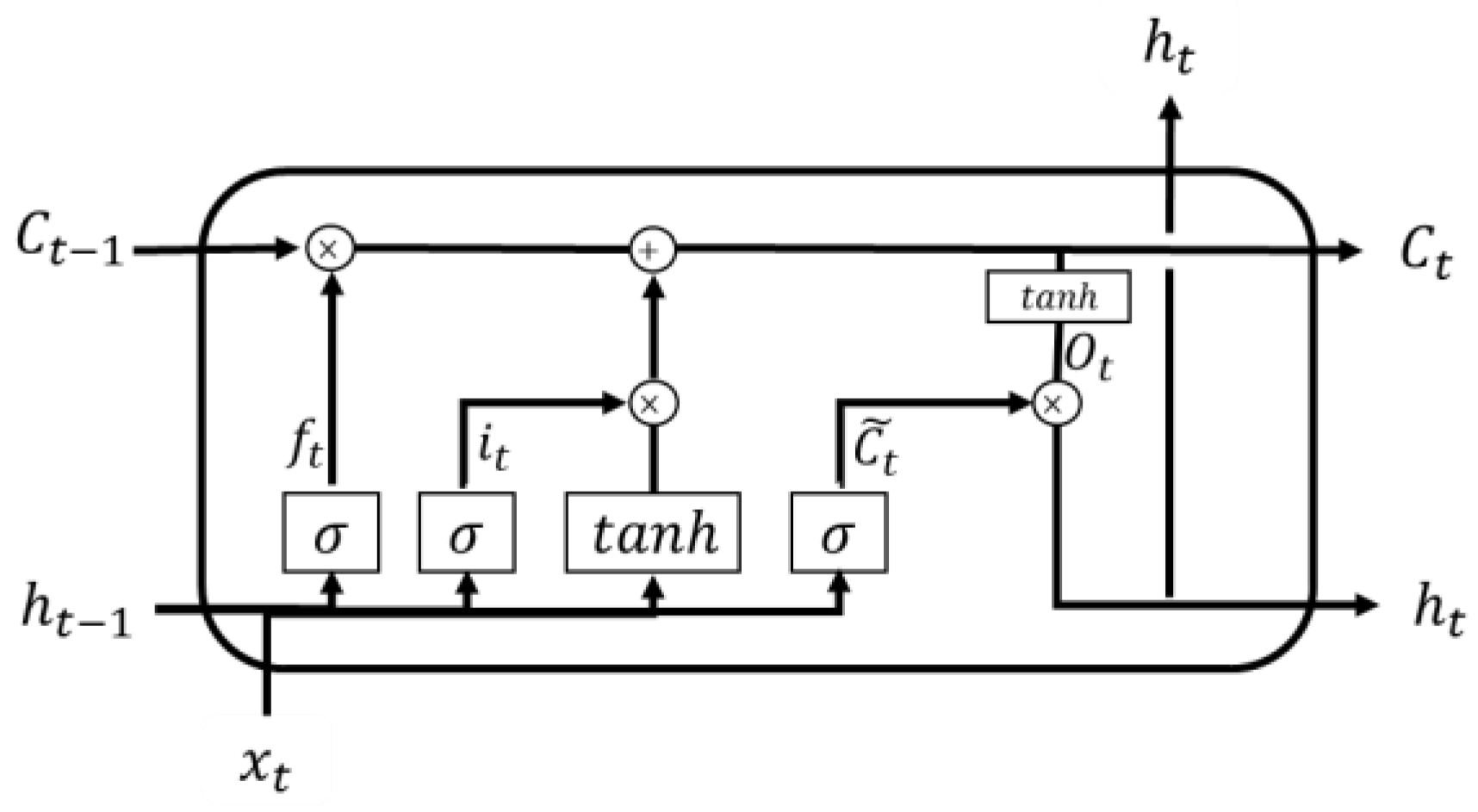
The input sequence of LSTM based on the attention mechanism is the data of rainfall, phreatic line and deformation at n time points before the prediction time. The above data are from the database of Zijin Mining Company Limited [39]. Determining the optimal sequence input length is conducive to improving the model accuracy and calculation speed [40]. The lag order is determined by the h-order lagging autocorrelation coefficient method as follows:

$$r_h={{\displaystyle \sum }}_{i=1}^{n-h}\frac{\left(x_i-\overline{x}\right)\left(x_{i+h}-\overline{x}\right)}{{{\displaystyle \sum }}_{i=1}^n{\left(x_i-\overline{x}\right)}^2}$$

(2)

where $x_i$ is the displacement, $\overline{x}$ is the average displacement, h is the lag order, and $r_h$ is the autocorrelation coefficient of the lag h order.

2.1.3. LSTM Network

LSTM is a neural network with the ability to memorize long- and short-term information. LSTM was proposed in 1997 [41] and has been improved and promoted recently [42]. LSTM can learn long-term dependent information and avoid the gradient vanishing of the traditional recurrent neural network (RNN). The internal structure of the LSTM unit is shown in Figure 2.

Compared with RNN, the input of the LSTM unit adds a hidden state $C_t$. The gates of LSTM at each sequence index position t include forget gate $f_t$, input gate $i_t$ and output gate $O_t$. The input vector of the LSTM unit is the input $X_t$ at the current time, the unit state $C_{t-1}$ at the previous moment and the hidden layer state $h_{t-1}$ at the previous moment. Forget gate and input gate are used to update the unit state and the output gate calculates the current hidden layer state $h_t$. The output is the unit state $C_t$ at the current moment with the hidden layer state $h_t$ at the current moment. The calculation equations of forget gate, input gate and output gate are as follows:

$$f_t=\sigma \left(W_f.[h_{t-1},x_t\right]+b_f)$$

(3)

$$i_t=\sigma \left(W_i.[h_{t-1},x_t\right]+b_i)$$

(4)

$$o_t=\sigma \left(W_o.[h_{t-1},x_t\right]+b_o)$$

(5)

where $W_f$, $W_i$, $W_o$ and $b_f$, $b_i$ and $b_o$ are the weight coefficient matrices and bias vectors, respectively, corresponding to each gate and $\left[h_{t-1},x_t\right]$ is the result of merging the state of the hidden layer and the input vector of the current layer. $\sigma$ is the Sigmoid activation function. $C_t$ consists of two parts that the first part is the product of $C_{t-1}$ and the output of forget gate and the second part is the product of $\widetilde{c_t}$ and $i_t$ of the input gate.

$$\widetilde{c_t}=\mathit{tanh}\left(w_c\cdot \left[h_{t-1},x_t\right]+b_c\right)$$

(6)

$$C_t=f_t\ast C_{t-1}+i_t\ast \widetilde{C_t}$$

(7)

where $h_t$ is the output of the LSTM unit at the current moment.

$$h_t=O_t\ast \mathit{tanh}\left(c_t\right)$$

(8)

where * is the Hadamard product. That is, the new matrix element is defined as the product of the corresponding elements of matrices A and B, and tanh is the hyperbolic tangent activation function.

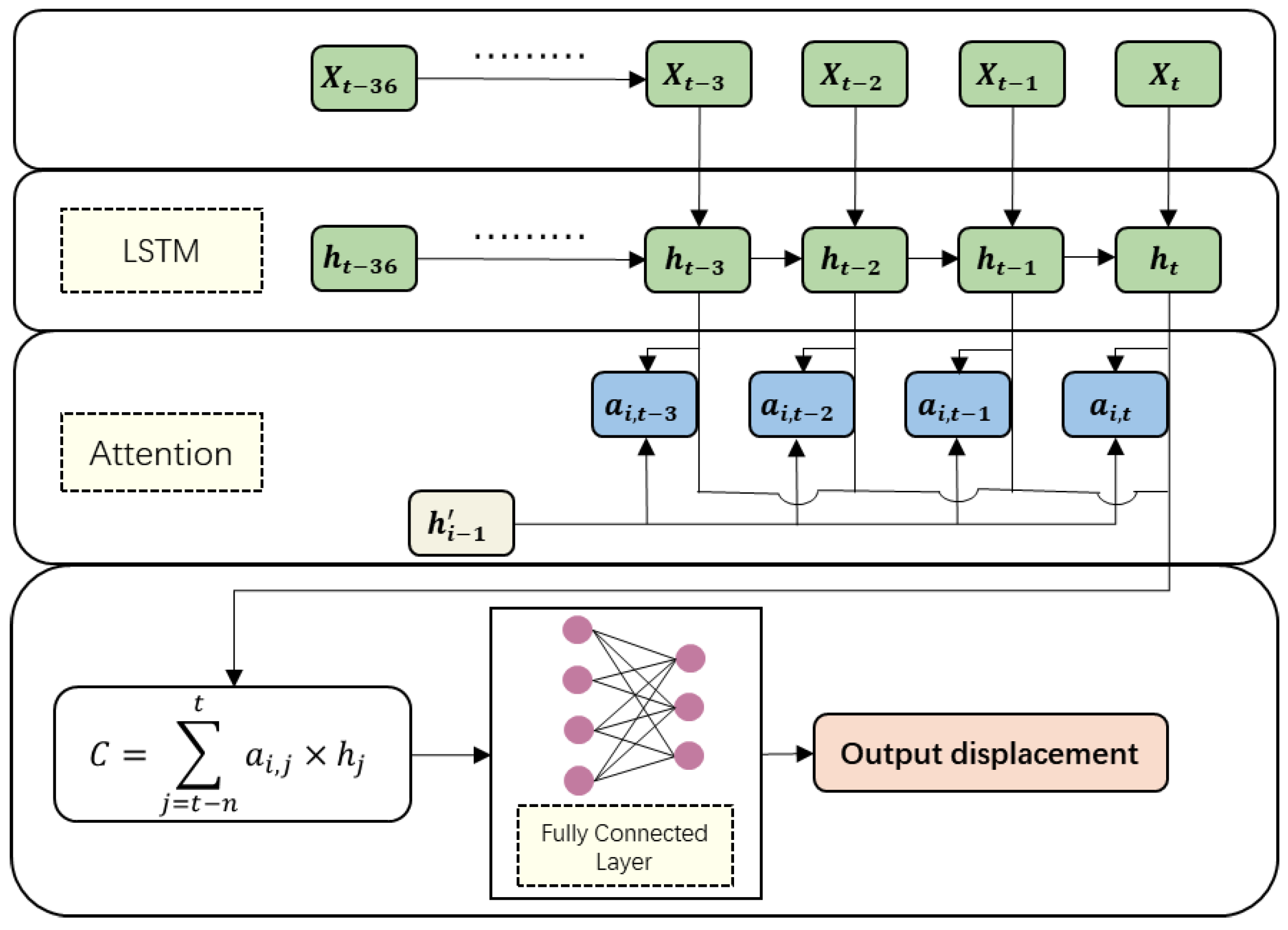
2.1.4. Attention Mechanism

This study introduces the attention mechanism based on LSTM to selectively learn these intermediate states through training models. The attention mechanism comes from the human learning process, in which a certain part of our learning always appears to be the most important content. To speed up learning efficiency and improve accuracy, we focus our attention on that part of the information and suppress other irrelevant information in the re-learning process. The weights, which are assigned by the attention mechanism to the input sequence, can determine the most relevant aspects that affect the prediction data, thus improving prediction accuracy. The attention mechanism can effectively improve the situation in which the LSTM loses information because of long sequences, and simultaneously replace the original method of randomly assigning weights with that of assigning probabilities [43].

2.1.5. Prediction Model Structure

The LSTM model outputs intermediate results according to the input sequence. The attention mechanism calculates different weights according to the importance of each item of the intermediate results to highlight the critical moments, overcomes the limitation that the LSTM model can only generate fixed-length vectors and improves prediction performance. In addition, calculating the intermediate results through the LSTM prediction model based on the attention mechanism facilitates a better understanding of the internal operation mechanism of the model and how the weight vector of the intermediate process affects the final result. Figure 3 shows the structure of the attention-LSTM-based tailings dam deformation prediction model.

In Figure 3, $X_{t-36},\dots ,X_{t-3},X_{t-2},X_{t-1},X_t$ is the 36 input sequences before the prediction time, $h_{t-36},\dots ,h_{t-3},h_{t-2},h_{t-1},h_t$ is the hidden layer state and $a_{i,t-3}\dots a_{i,t-2},a_{i,t-1},a_{i,t}$ is the attention coefficient. The calculation formula is as follows:

$$e_{ij}=v\mathit{tanh}\left(w\cdot h_j+U\cdot h_{i-1}^{\prime },+b\right)$$

(9)

$$a_{ij}=\frac{\mathit{exp}\left(e_{ij}\right)}{{{\displaystyle \sum }}_{k=t-n}^t\mathit{exp}\left(e_{ik}\right)}$$

(10)

$$c={{\displaystyle \sum }}_{j=t-n}^t{a}_{ij}{h}_j$$

(11)

The attention coefficient $a_{ij}$ is calculated by the relation score $e_{ij}$ and $e_{ij}$ is the relation score of the middle layer state. The larger the value of $e_{ij}$, the larger the corresponding attention coefficient, and then the result of the multiplication and superposition of the hidden layer $h_j$ and the attention coefficient $a_{ij}$ is input into the decoder to obtain the displacement prediction result at the next moment.

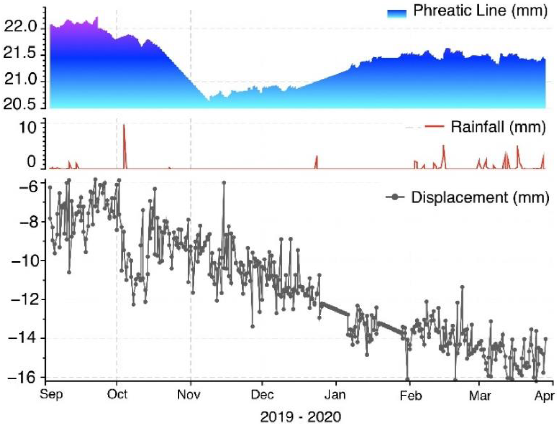
2.2. A Tailing Dam Study

2.2.1. Introduction of Background

The Zijin Mountain gold-copper ore mine is located 14.6 km north of Longyan City, Fujian Province, China. Longyan City is on the west coast of the Taiwan Strait and in the southwestern part of Fujian Province (24°23′ N–26°02′ N, 115°51′ E–117°45′ E). The average elevation of the whole city is 652 m. Longyan City has a subtropical maritime monsoon climate, where the average temperature is 18.7 °C~21.0 °C and the average precipitation is 1031–1369 mm. The Zijin Mountain gold-copper ore mine is one of the mega non-ferrous metal deposits discovered and proven in the 1980s in China. It has been proven gold resource reserves of more than 300 tons and copper resource reserves of more than 5 million tons. The mine became the only world-class mega-gold mine in China at the beginning of the 20th century and has a large tailings pond [44].

The current existing monitoring systems of the Zijin Mountain Gold-Copper Ore mainly include GPS monitoring, radar monitoring, GNSS online monitoring, groundwater level monitoring, rainfall monitoring, etc. The displacement was directly influenced by the phreatic line and the lag of rainfall [45,46,47,48,49,50]. This study uses the deformation, rainfall and phreatic line of the Zijin Mountain tailings dam from 3 September 2019 to 29 March 2020 as a data set with a sampling frequency of 12 h. The data were collected at 417 moments, i.e., 208 days. Due to equipment failures at the monitoring sites, there are a large amount of missing data from before September 2019. In performing neural network model prediction, the selection of the test set requires the selection of real data so that the optimal model parameters can be obtained by the back propagation algorithm of errors from the test set. Therefore, by recording data every 12 h, the 208 days were extended to 417 moments to simulate a complete tailings dam scenario lasting 1 year under rainy and dry seasons and considering heavy rainfall conditions for resolving the missing data problem. To test the long-term prediction effect, the prediction time was set as 30 days and the data for the first 178 days were the training set and the data for the last 30 days were the test set. The distribution map of the monitoring points is as shown in Figure 4, where the dam displacement is in the X direction as an example.

The data above are selected for the samples of hyperparameters for training the LSTM network based on the attention mechanism. Data preprocessing includes missing value interpolation and outlier handling [51]. The outliers are processed by the boxplot method and they were removed and treated as missing values afterward. For the single missing value, the mean imputation method is adopted, while the linear interpolation method is used for continuous missing data [52]. Because the original data are not suitable for direct input into the model for training, we need to preprocess the original data, such as by outlier processing and missing value imputation.

2.2.2. The Outlier Data Processing

We use boxplot to deal with outliers, with the upper quartile symbol setting to U, indicating that samples greater than U in the dataset account for 1/4 of the total, and the lower quartile symbol set to L, indicating that samples less than L in the dataset account for 1/4 of the total. We define IQR as the difference between the upper and lower quartiles: IQR = U − L. Then the upper bound of the normal range is $\mathrm{U}+1.5\ast \mathrm{IQR}$ and the lower bound is $\mathrm{L}-1.5\ast \mathrm{IQR}$. A value greater than the upper bound or less than the lower bound is considered as an outlier [53]. This study regards outliers as missing values that are processed by the missing value processing method.

2.2.3. Missing Value Date Processing

In addition to the missing values from deleting outliers, there are also missing data caused by the failure of data collection equipment, storage media or transmission media, or by human factors that are omitted, lost or not recorded. Missing data may cause the system to lose a great deal of useful information, making the uncertainty in the system more pronounced and the deterministic component of the system more difficult to grasp. Besides, the data containing null values will confuse the data mining process, leading to unreliable outputs and other results. Missing values can be classified as missing completely at random (MCAR), missing at random (MAR) and missing not at random (MNAR) in terms of distribution [54]. In time series analysis, the following methods are commonly used for missing value processing: mean imputation, maximum likelihood (ML), multiple imputation (MI), linear interpolation and k-nearest neighbor (KNN) [20,55,56].

The phreatic line is a continuous time series and there exist both individual and continuous missing data. For the single missing data, we use the method of mean imputation: the sensor monitoring data are sorted in the sequence at the same time interval, and NA is defined as the null value. The equation for imputing the single missing value is:

$$NA=\frac{Tim{e}_A+Tim{e}_B}{2}$$

(12)

where $Tim{e}_A$ represents the non-null data value before the missing value and $Tim{e}_B$ represents the non-null data value after the missing value. For continuous missing data, this paper adopts the linear interpolation method, which is a kind of missing data interpolation method, and its interpolation function is a first-order polynomial.

2.2.4. Data Normalization

Different data variables have different data formats and units. Many large-scale variables will cause the model to ignore small-scale variables and lose this part of information, thereby affecting the results of data analysis. To eliminate the dimensional influence between the indicators, the data is processed by the min-max normalization method:

$$x_i^{\prime }=\frac{x_i-x_{min}}{x_{max}-x_{min}}$$

(13)

where $x_i$ is the original variable, $x_{max}$ and $x_{min}$ are the maximum and minimum values in the current variable sequence, respectively.

3. Results

3.1. Data Analysis and Processing

For the missing rainfall data, the historical rainfall data of Shanghang County (25°20 N, 116°39 E) collected from the China Meteorological Data Service Center (CMDC) were adopted to interpolate the database. The outliers are processed by the boxplot. The boxplot of phreatic line and tailings dam deformation are as shown in Figure 5 and the results after processing show that point 39 is anomalous. After the outlier is deleted, the missing data that stems from the outlier deletion are processed by the missing value processing method. At the same time, the continuous missing data are processed by linear interpolation and the results are as shown in Figure 6.

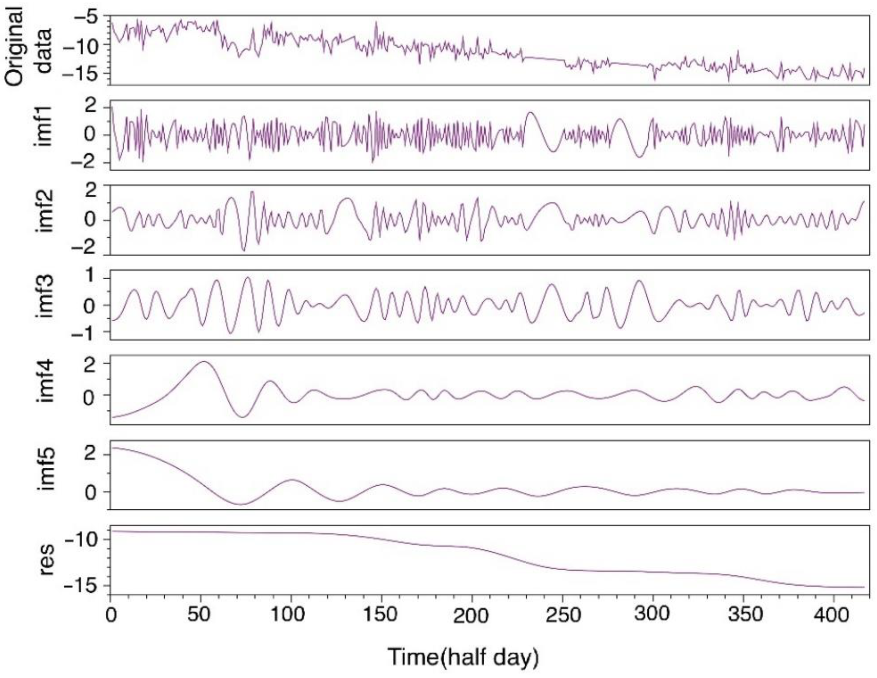
3.2. EMD Reorganization of Absolute Deformation of the Tailings Dam

The deformation time series data is decomposed into five scales of IMFs and one residual term by EMD to reduce the nonlinearity and instability of the displacement series (Figure 7). Considering the influence of IMFs and residual term on the original data, we perform the augmented Dickey–Fuller test (ADF test) and the method of component identification, i.e., the Pearson correlation coefficient method on the stationarity of the sequence. After comprehensively considering the results of the ADF test and component identification, the decomposed IMFs and residual term are used as individual components or a combination of components to predict the original data.

3.2.1. Stationarity Test

The stationarity test is performed on IMF₁ to IMF₅ and the residual term. The ADF test can determine whether unit roots exist in the sequence. Under a stationary sequence, there is no unit root, and vice versa [57]. It is specified here that the sequence can be considered as stationary when the p-value of the ADF test is lower than 0.05; otherwise, it is nonstationary. After the ADF test, the test statistic and p-value of IMF₁ to IMF₅ and the residual term are as shown in

Table 1. Stationarity test of IMF₁~IMF₅, residual term and original data.

	Original Data	IMF1	IMF2	IMF3	IMF4	IMF5	Residual Term
Test Statistic	0.900	−8.065	−7.577	−7.348	−4.637	−4.225	−0.641
p-value	0.788	0.000	0.000	0.000	0.000	0.001	0.861
Stationarity	N	Y	Y	Y	Y	Y	N

. Y represents the sequence is stationary, and N represents the sequence is nonstationary. Because the original displacement data is nonstationary, the residual term and the original sequence are nonstationary after EMD, and IMF₁~IMF₅ are all stationary sequences.

3.2.2. Component Identification

The degrees of correlation between each IMF component of the tailings dam deformation and the original data are as shown in

Table 2. Pearson correlation coefficient between IMF₁~IMF₅, residual term and the original data.

IMFs and Residual Term	IMF1	IMF2	IMF3	IMF4	IMF5	Residual Term
Pearson Correlation Coefficient	0.2077	0.1264	0.1453	0.1470	0.4599	0.9122

(which are calculated in accordance with the Pearson correlation coefficient method [58].

After the Pearson correlation coefficient test, IMF_1, IMF₅ and the residual term are more correlated with the original series, which indicates that the IMF₁ and IMF₅ components and the residual term are more correlated with the original data. While the rest of the IMF₂, IMF₃ and IMF₄ components are less correlated with that. After comprehensive consideration of the two methods, the ADF test and component identification, the IMF₁-IMF₅ components and the residual term are combined as follows.

We take the three components IMF₁, IMF₅ and the residual term, which are higher correlated with the original time series or have the same stationarity as that, as independent components and combine the remaining three components (IMF₂, IMF₃ and IMF₄) to form a new component IMF₆. IMF₁, IMF₅, the residual term and the newly formed component IMF₆ are input are into the attention-mechanism-based LSTM network model for prediction, respectively. Then the predicted value of each group of components and the predicted value of the trend are added with equal weight. Finally, the prediction result of the deformation of the tailings dam is obtained.

3.3. Input Sequence

In the study of the temporal relationship between rainfall and phreatic line, Wang [59] found that the relationship is $Y=1.0175X^{1.6515}$, where Y is the lag time (d) of groundwater recharged by precipitation infiltration and X is the groundwater depth (m). The maximum value of lag h was determined to be 155 days, and then the lagged autocorrelation coefficients from 1 to 155 days were calculated sequentially, as shown in Figure 8. The optimal lag order is determined to be 18; that is, the historical data of the first 18 days are the best for the prediction effect. Since the data are taken every 12 h, the length of the input sequence is selected as 36. Based on the previous judgment, the format of the input sequence is chosen to be 36 × 3. All input data involve rainfall, phreatic line, and tailings dam deformation at 36 time points before predicting deformation.

3.4. Model Parameter Setting

The parameters of the attention-LSTM prediction model in this study are batch size = 64, SEQ_LEN = 36 and the prediction step size, which equals 1. The input contains data of rainfall, displacement and phreatic line, and the structure of each type data is 36 time points in three columns. LSTM consists of two layers and each layer contains 64 neurons. The dense layer is connected behind both layers to enhance the learning data characteristics. At the same time, a dropout layer is inserted between the LSTM layers to prevent the model from overfitting. At present, most model optimizers use the adaptive gradient (AdaGrad), root mean square propagation (RMSProp), and adaptive momentum estimation (Adam) [60] methods. Among them, Adam is an effective gradient-based stochastic optimization algorithm. The advantages of the AdaGrad and RMSProp algorithms can be exploited by this fusion algorithm, which has high computational efficiency and low memory requirements in practical applications [61]. Therefore, the Adam optimization algorithm is selected in this study, and Adam is used as the optimizer. The software and version used for LSTM in this study are PyCharm 2020.2.5 (Community Edition) and Python 3.8, respectively.

Figure 9 shows the effect of tailings dam deformation prediction.

Compared with the control model, the LSTM model with attention mechanism after EMD decomposition is closer to the measured deformation value. In addition, the hysteresis mutation prediction on 7 and 16 March is more realistic. This is because the attention mechanism assigns different weights to the previous rainfall and phreatic line and inputs them into the LSTM; then the test set can read the mutation information of the previous rainfall and phreatic line. By contrast, the multiple regression model has fewer independent variables and has no hysteresis; therefore, the prediction error is large. Compared with the model proposed in this study, the prediction error of the support vector machine (SVM) model increases rapidly with the increase of the number of days. This result reflects that if the SVM model wants to achieve a good prediction effect in the long term, it is necessary to select the correct kernel function and dynamically adjust it according to the data. At the same time, the prediction accuracy of the LSTM model does not reach the effect of the EMD-LSTM model, indicating that the EMD method can improve the accuracy of the model prediction to a certain extent.

For the deformation prediction of the tailings dam, two common indicators for evaluating the accuracy of the model are selected: root mean square error (RMSE) and mean absolute deviation (MAE) [62,63]. RMSE evaluates the accuracy of the prediction results. The smaller the value of RMSE, the better the accuracy of the prediction model; MAE is the average of the absolute value of deviations between all single observations and the prediction values. The closer the indicator is to 0, the higher the prediction accuracy.

$$RMSE=\sqrt{\frac{1}{n}{\displaystyle \sum }_{i=1}^n{\left(y_i-q_i\right)}^2}$$

(14)

$$MAE=\frac{1}{n}{\displaystyle \sum }_{i=1}^n|y_i-q_i|$$

(15)

where $y_i$ represents the prediction value of the tailings dam deformation, $q_i$ indicates the observed value of the tailings dam deformation and n is the sample capacity of the test set. In this research, n = 60. The test set of this model is 30 days. The prediction accuracies of the absolute displacement of the tailings dam are as shown in

Table 3. The prediction accuracy of absolute displacement of the tailings dam.

	Day	EMD-Attention-LSTM	EMD-LSTM	EMD-ARIMA	Multiple Regression	LSTM	SVM
RMSE	1	0.144	0.371	0.529	4.760	0.470	0.296
	5	0.183	0.351	0.410	4.398	0.411	0.496
	10	0.549	0.934	1.049	4.673	0.945	1.167
	15	0.553	0.835	0.992	4.675	0.907	1.129
	20	0.607	0.865	1.010	4.844	0.893	1.222
	25	0.625	0.898	1.053	5.237	0.908	1.208
	30	0.729	0.955	1.120	4.937	0.970	1.285
MAE	1	0.157	0.524	0.676	6.731	0.642	0.384
	5	0.215	0.439	0.536	6.080	0.462	0.573
	10	0.509	0.992	1.059	6.455	0.955	1.078
	15	0.555	0.906	1.035	6.455	0.950	1.145
	20	0.636	0.945	1.054	6.668	0.934	1.274
	25	0.664	0.996	1.111	6.747	0.965	1.294
	30	0.770	1.068	1.207	6.801	1.063	1.394

.

The prediction results show that in the case of considering rainfall and infiltration lines, the proposed model in the paper is compared with EMD-LSTM, the RMSE and MAE values on the 1st day decreased by 0.227 and 0.367, respectively, and on the 30th day the percentages of RMSE and MAE decreased by 23.66% and 27.9%, respectively. This is because the attention mechanism helps to improve the prediction accuracy through the weight distribution between influencing factors. Compared to the model EMD-ARIMA, the RMSE and MAE also drop significantly; the reason is that the prediction error of the ARIMA model increases over time. Compared with commonly used multiple regression models, RMSE and MAE are reduced by 4.616 and 6.574, respectively, and the prediction accuracy is significantly improved.

4. Discussion

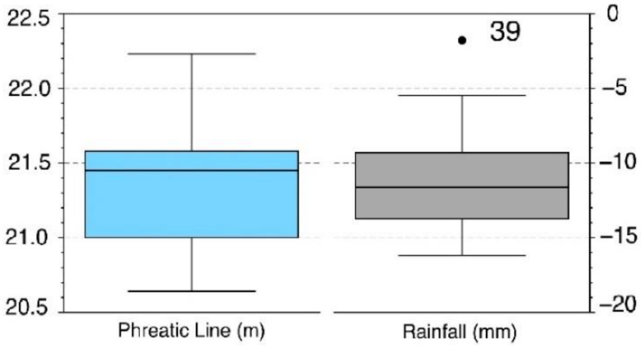
4.1. Factor Analysis

Through the exploration of significance tests on the regression coefficient of the multiple regression model from the comparison model,

Table 4. Significance test on regression coefficient of the comparison model.

Multiple Regression Model	Unstandardized Coefficient B	Standard Error	t	Significance
Constant	−22.890	5.631	−4.065	0.000
Phreatic line	0.524	0.263	1.991	0.047
rainfall	−0.392	0.152	−2.588	0.010

shows the significance test values of the rainfall and phreatic line are 0.047 and 0.01, respectively. They are less than 0.05, indicating that the rainfall and phreatic line significantly affect the absolute deformation of the tailings dam in the X-direction. Furthermore, compared with the phreatic line, the effect of rainfall on the deformation of the tailings dam is more prominent.

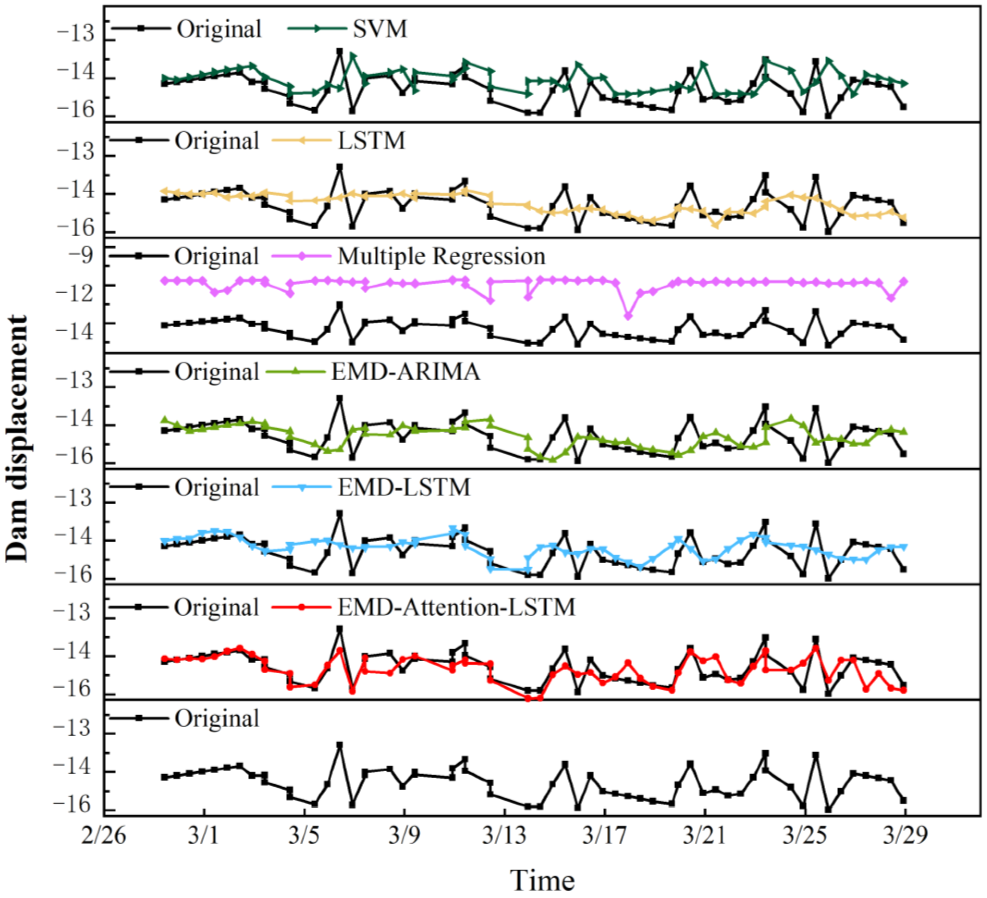
4.2. Model Application

The method above is used to fit the deformation of the tailings dam in Y and Z directions, and the training and test sets are divided in the same proportion as the X-direction. The prediction results of the test set are as shown in Figure 10. The RMSE of predicting the Y-direction deformation of the tailings dam for 7 days is less than 0.585 and the relative error of predicting the deformation for 30 days is controlled at 0.588. The prediction error in the Z-direction of the deformation of the tailings dam increases by 0.121 from 0.022. The short-term prediction accuracy of this method is high. The long-term one, although descending, is still in line with expectations. The model has an outstanding long-term prediction effect in Y- and Z-directions, and better in the Z-direction. The absolute displacement prediction in three directions can be used as engineering examples.

The horizontal displacement of the tailings dam is divided into two directions, X-direction and Y-direction, and the Z-direction is the vertical settlement data of the tailings dam. In the initial stage of tailings dam deformation, vertical settlement dominates and horizontal displacement is only an additional effect of vertical settlement. The horizontal displacement of the tailings dam is affected by the lag of rainfall and phreatic line. The increase of rainfall and the change of phreatic line make the oscillation and instability of the horizontal deformation rate increase, which makes the prediction of horizontal displacement more difficult than that of the vertical direction. However, as rainfall occurs, the phreatic line changes and time passes, the downstream part of the dam tends to stabilize because of its upper load, so the magnitude of vertical deformation gradually decreases and stability increases; compared with horizontal displacement, the prediction accuracy of vertical settlement is higher.

To emphasize the reproducibility of the method, the displacement of the monitoring point on the east side of the tailings dam is predicted in Figure 11 and Figure 12 (the monitoring point is as shown in Figure 4). Figure 11 shows that for the evaluation index RMSE, the prediction error range in the X-direction is 0.278~0.758 and the prediction error of the other two directions is less than 0.932 and 0.772. For the evaluation index MAE, the prediction error range in the X-direction is 0.365~0.816 and the prediction error of the other two directions is less than 1.009 and 0.723.

As shown in Figure 12, by using the EMD-attention-LSTM method again, this model again achieves excellent prediction results in the X-, Y- and Z-directions of the new monitoring point. In addition, by repeatability experiments, the accuracy evaluation indicators RSEM and MAE of the prediction effect of the model in the Z-direction are at least 0.128 and 0.141, respectively, which proves that the method has applicability in the deformation prediction of the tailings dam and is convenient for promotion.

One of the limitations of this study is that the lag order of this method is fixed. If the lag order is dynamically adjusted according to the historical data, it may bring better effect. In addition, the method proposed in this study has only been verified with the tailing dam displacement prediction and has not been applied to other scenarios. Finally, LSTM model parameter training requires plenty of time and has high requirements for hardware.

5. Conclusions

(1)

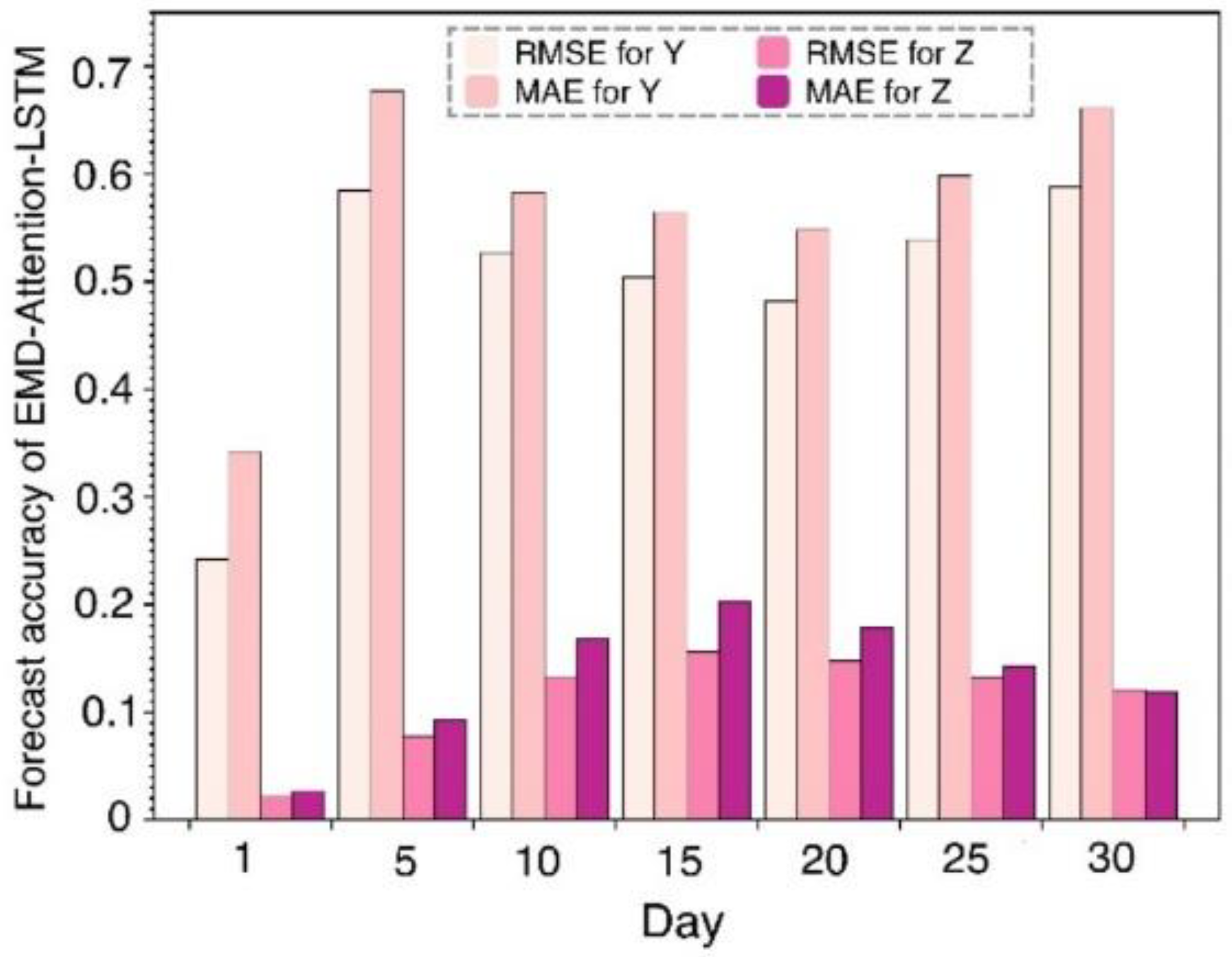
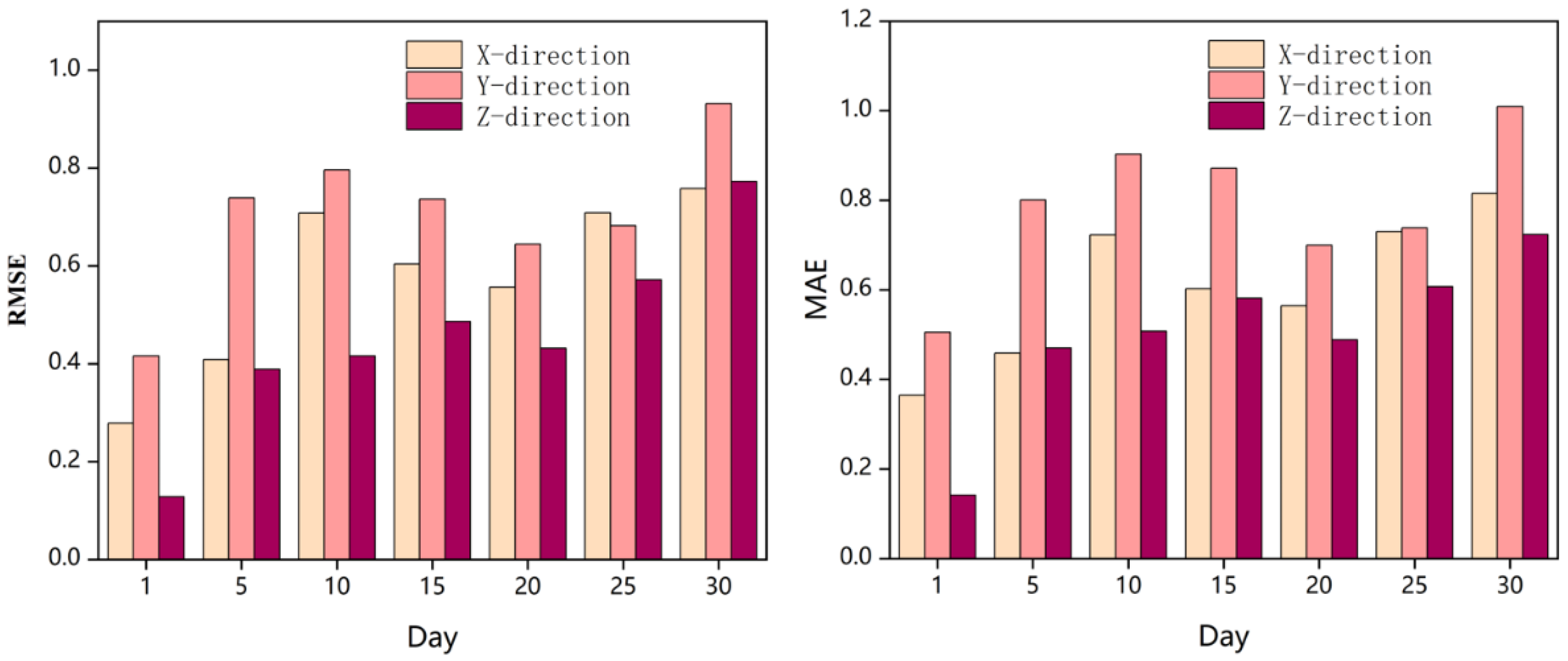
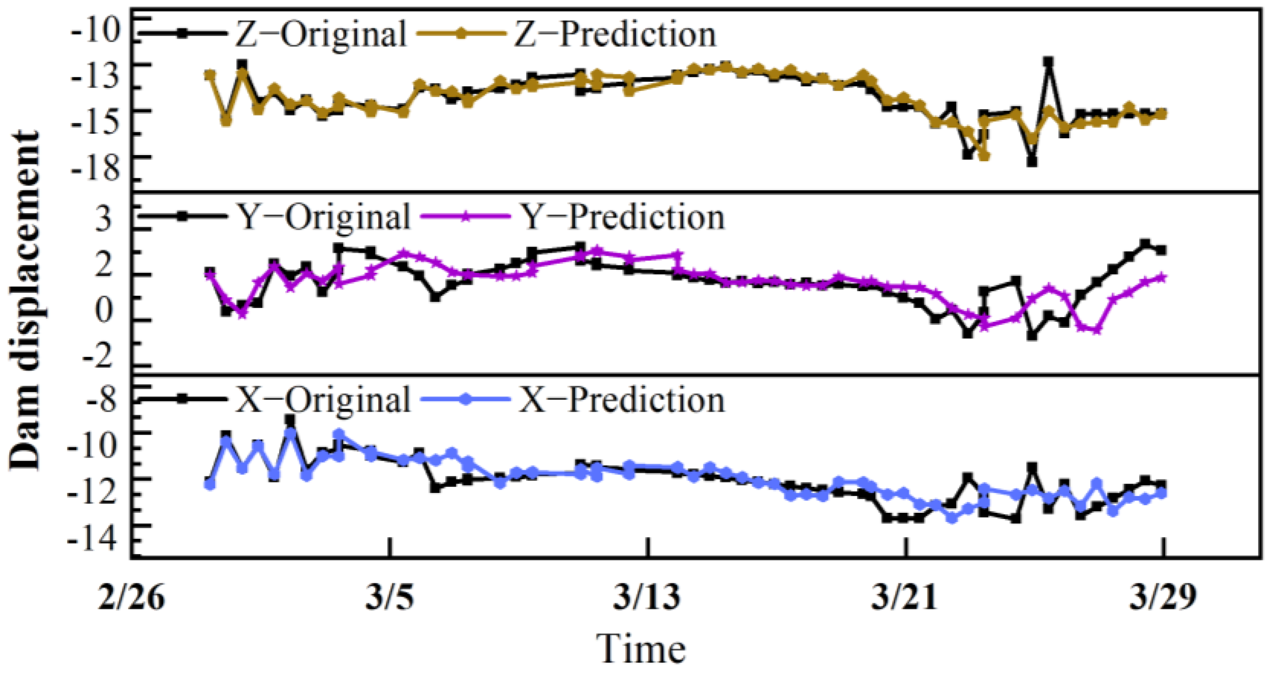
In this study, the EMD-attention-LSTM neural network model is proposed. Compared with the control models, this model achieves higher accuracy in the prediction of tailings dam deformation under the influence of rainfall and phreatic line, and also has good performance in multiple directions. The prediction effect reflects the universality of this model in the prediction of tailings dam deformation. This method is suitable for dam deformation prediction under the influence of rainfall and phreatic line and has engineering significance.

(2)

The LSTM model used in this study effectively avoids the problem of gradient disappearance and gradient explosion, while the model considers the lag to better reflect the delayed impact of external factors on the dam deformation in real situations.

(3)

Compared with a single LSTM model, the addition of the attention mechanism takes into account the characteristics of the input variables and the long-term dependence of the time series, which improves the prediction accuracy of the dam displacement.

(4)

The significance test reveals that atmospheric rainfall and the change of phreatic line in the tailings dam will accelerate the tailings dam deformation process, and the change of phreatic line has a more significant effect on tailings dam deformation.

Although the proposed model has improved the accuracy of tailings dam displacement prediction, there is still room for further refinements. Subsequent studies will focus on the following aspects: (1) the proposed model integrating statistics and machine learning and (2) reducing the requirements of a large amount of data to adjust the hyperparameters. In future research, we will collect more different types of tailings dam monitoring data to further expand the application scenarios of the model.

References

1. Burritt, R.L.; Christ, K.L. Water risk in mining: Analysis of the Samarco dam failure. J. Clean. Prod. 2018, 178, 196–205. [Google Scholar] [CrossRef]
2. Kossoff, D.; Dubbin, W.E.; Alfredsson, M.; Edwards, S.J.; Macklin, M.G.; Hudson-Edwards, K.A. Mine tailings dams: Characteristics, failure, environmental impacts, and remediation. Appl. Geochem. 2014, 51, 229–245. [Google Scholar] [CrossRef] [Green Version]
3. Xu, Z. Mineral processing technology (5th edition): B.A. Wills Pergamon Press, Oxford, UK, 1992, 855 pps. Price £29.95 (flexicover); £75 (hardback) ISBN 0 08041872 4 F (flexicover); 0 08041885 6 (hardback). Miner. Eng. 1994, 7, 427–428. [Google Scholar] [CrossRef]
4. Barrie, S.; Baker, E.; Howchin, J.; Matthews, A. Chapter XVI Investor Mining And Tailings Safety Initiative. In Towards Zero Harm: A Compendium of Papers Prepared for the Global Tailings; GRID-Arendal: Arendal, Norway, 2020; p. 216. [Google Scholar]
5. Hancock, G.R.; Loch, R.J.; Willgoose, G.R. The design of post-mining landscapes using geomorphic principles. Earth Surf. Process. Landf. 2003, 28, 1097–1110. [Google Scholar] [CrossRef]
6. Beauchemin, S.; Langley, S.; MacKinnon, T. Geochemical properties of 40-year old forested pyrrhotite tailings and impact of organic acids on metal cycling. Appl. Geochem. 2019, 110, 104437. [Google Scholar] [CrossRef]
7. Xuecheng, S.; Jianxu, W.; Xinbin, F. Distribution and Potential Environmental Risk of Mercury and Arsenic in Slag, Soil and Water of Danzhai Mercury Mining Area, Guizhou Province, China. Asian J. Ecotoxicol. 2014, 6, 1173–1180. [Google Scholar] [CrossRef]
8. Dong, L.; Deng, S.; Wang, F. Some developments and new insights for environmental sustainability and disaster control of tailings dam. J. Clean. Prod. 2020, 269, 122270. [Google Scholar] [CrossRef]
9. Lang, X.Z.; Xu, T.L.; Huang, X.J.; Du, H.C.; Song, H.Y. PCA and neural network are used to predict underground water level of tailings dam. Hydrogeol. Eng. Geol. 2014, 2, 13–17. [Google Scholar]
10. Li, Z.W.; Hu, Z.Q. Stability analysis of tailings dam based on seepage theory. J. Hydraul. Archit. Eng. 2010, 8, 56–59. [Google Scholar]
11. Godt, J.W.; Baum, R.L.; Lu, N. Landsliding in partially saturated materials. Geophys. Res. Lett. 2009, 36, L02403. [Google Scholar] [CrossRef]
12. Sun, H.; Pan, P.; Lu, Q.; Zhenlei, W.; Xie, W.; Zhan, W. A case study of a rainfall-induced landslide involving weak interlayer and its treatment using the siphon drainage method. Bull. Eng. Geol. Environ. 2018, 78, 4063–4074. [Google Scholar] [CrossRef]
13. Wei, Z.; Lü, Q.; Sun, H.; Shang, Y. Estimating the rainfall threshold of a deep-seated landslide by integrating models for predicting the groundwater level and stability analysis of the slope. Eng. Geol. 2019, 253, 14–26. [Google Scholar] [CrossRef]
14. Rosone, M.; Ziccarelli, M.; Ferrari, A.; Farulla, C. On the reactivation of a large landslide induced by rainfall in highly fissured clays. Eng. Geol. 2018, 235, 20–38. [Google Scholar] [CrossRef]
15. Belmokre, A.; Mihoubi, M.K.; Santillan, D. Seepage and dam deformation analyses with statistical models: Support vector regression machine and random forest. In Proceedings of the 3rd International Conference on Structural Integrity, ICSI 2019, Funchal, Portugal, 2–5 September 2019; Volume 17, pp. 698–703. [Google Scholar] [CrossRef]
16. Zhao, E.; Wu, C. Centroid deformation-based nonlinear safety monitoring model for arch dam performance evaluation. Eng. Struct. 2021, 243, 112652. [Google Scholar] [CrossRef]
17. Xu, C.; Yue, D.; Deng, C. Hybrid GA/SIMPLS as alternative regression model in dam deformation analysis. Eng. Appl. Artif. Intell. 2012, 25, 468–475. [Google Scholar] [CrossRef]
18. Jung, I.-S.; Berges, M.; Garrett, J.H.; Poczos, B. Exploration and evaluation of AR, MPCA and KL anomaly detection techniques to embankment dam piezometer data. Adv. Eng. Inform. 2015, 29, 902–917. [Google Scholar] [CrossRef] [Green Version]
19. Zhang, J.; Tang, H.; Tannant, D.D.; Lin, C.; Xia, D.; Liu, X.; Zhang, Y.; Ma, J. Combined forecasting model with CEEMD-LCSS reconstruction and the ABC-SVR method for landslide displacement prediction. J. Clean. Prod. 2021, 293, 126205. [Google Scholar] [CrossRef]
20. Liu, Y.; Feng, X. Prediction of dam horizontal displacement based on CNN-LSTM and attention mechanism. Acad. J. Archit. Geotech. Eng. 2021, 3, 6. [Google Scholar]
21. Le, X.-H.; Ho, H.V.; Lee, G.; Jung, S. Application of Long Short-Term Memory (LSTM) Neural Network for Flood Forecasting. Water 2019, 11, 1387. [Google Scholar] [CrossRef] [Green Version]
22. Han, Y.; Zhou, R.; Geng, Z.; Chen, K.; Wang, Y.; Wei, Q. Production prediction modeling of industrial processes based on Bi-LSTM. In Proceedings of the 2019 34rd Youth Academic Annual Conference of Chinese Association of Automation (YAC), Jinzhou, China, 6–8 June 2019; pp. 285–289. [Google Scholar] [CrossRef]
23. Huo, Y.; Yan, Y.; Du, D.; Wang, Z.; Zhang, Y.; Yang, Y. Long-Term Span Traffic Prediction Model Based on STL Decomposition and LSTM. In Proceedings of the 2019 20th Asia-Pacific Network Operations and Management Symposium (APNOMS), Matsue, Japan, 18–20 September 2019; pp. 1–4. [Google Scholar] [CrossRef]
24. Lin, H.-M.; Chang, S.-K.; Wu, J.-H.; Juang, C.H. Neural network-based model for assessing failure potential of highway slopes in the Alishan, Taiwan Area: Pre- and post-earthquake investigation. Eng. Geol. 2009, 104, 280–289. [Google Scholar] [CrossRef]
25. Chang, S.-K.; Lee, D.-H.; Wu, J.-H.; Juang, C.H. Rainfall-based criteria for assessing slump rate of mountainous highway slopes: A case study of slopes along Highway 18 in Alishan, Taiwan. Eng. Geol. 2011, 118, 63–74. [Google Scholar] [CrossRef]
26. Li, Q.; Geng, J.; Song, D.; Nie, W.; Saffari, P.; Liu, J. Automatic Recognition of Erosion Area on the Slope of Tailings Dam Using Region Growing Segmentation Algorithm. Arab. J. Geosci. 2022, 15, 438. [Google Scholar] [CrossRef]
27. Chen, W.-B.; Liu, W.-C.; Hsu, M.-H. Comparison of ANN approach with 2D and 3D hydrodynamic models for simulating estuary water stage. Adv. Eng. Softw. 2012, 45, 69–79. [Google Scholar] [CrossRef]
28. Chen, W.-B.; Liu, W.-C. Artificial neural network modeling of dissolved oxygen in reservoir. Environ. Monit. Assess. 2013, 186, 1203–1217. [Google Scholar] [CrossRef]
29. Chiang, S.; Chang, C.-H.; Chen, W.-B. Comparison of Rainfall-Runoff Simulation between Support Vector Regression and HEC-HMS for a Rural Watershed in Taiwan. Water 2022, 14, 191. [Google Scholar] [CrossRef]
30. Ren, Q.; Li, M.; Li, H.; Shen, Y. A novel deep learning prediction model for concrete dam displacements using interpretable mixed attention mechanism. Adv. Eng. Inform. 2021, 50, 101407. [Google Scholar] [CrossRef]
31. Yang, D.; Gu, C.; Zhu, Y.; Dai, B.; Zhang, K.; Zhang, Z.; Li, B. A Concrete Dam Deformation Prediction Method Based on LSTM With Attention Mechanism. IEEE Access 2020, 8, 185177–185186. [Google Scholar] [CrossRef]
32. Guo, H.Q.; Wu, Z.R.; Yang, J. Grey nonlinear time series combination model for rockfill dam deformation monitoring. J. Hohai Univ. 2001, 29, 51–55. [Google Scholar]
33. Yuan, R.; Su, C.; Cao, E.; Hu, S.; Zhang, H. Exploration of Multi-Scale Reconstruction Framework in Dam Deformation Prediction. Appl. Sci. 2021, 11, 7334. [Google Scholar] [CrossRef]
34. Xing, Y.; Yue, J.; Chen, C.; Cong, K.; Zhu, S.; Bian, Y. Dynamic Displacement Forecasting of Dashuitian Landslide in China Using Variational Mode Decomposition and Stack Long Short-Term Memory Network. Appl. Sci. 2019, 9, 2951. [Google Scholar] [CrossRef] [Green Version]
35. Xu, X.; Zhang, P.; Jiang, J. Dam Deformation Prediction Based on EMD-GAELM-ARIMA Algorithm. Comput. Mod. 2020, 0, 1–5. [Google Scholar] [CrossRef]
36. Li, M.; Wang, J. An Empirical Comparison of Multiple Linear Regression and Artificial Neural Network for Concrete Dam Deformation Modelling. Math. Probl. Eng. 2019, 2019, 7620948. [Google Scholar] [CrossRef] [Green Version]
37. Wu, Z.; Huang, N. Ensemble Empirical Mode Decomposition: A Noise-Assisted Data Analysis Method. Adv. Adapt. Data Anal. 2009, 1, 1–41. [Google Scholar] [CrossRef]
38. Yan, T.; Chen, B.; Cao, E.H.; Liu, Y.T. Prediction of Dam Deformation Using EEMD-ELM Model. J. Yangtze River Sci. Res. Inst. 2020, 37, 70. [Google Scholar] [CrossRef]
39. Nie, W.; Luo, M.; Wang, Y.; Li, R. 3D Visualization Monitoring and Early Warning System of a Tailings Dam—Gold Copper Mine Tailings Dam in Zijinshan, Fujian, China. Front. Earth Sci. 2022, 10, 800924. [Google Scholar] [CrossRef]
40. Nie, W.; Krautblatter, M.; Leith, K.; Thuro, K.; Festl, J. A modified tank model including snowmelt and infiltration time lags for deep-seated landslides in Alpine Environments (Aggenalm, Germany). Nat. Hazards Earth Syst. Sci. Discuss. 2016, 2016, 1. [Google Scholar] [CrossRef] [Green Version]
41. Hochreiter, S.; Schmidhuber, J. Long Short-Term Memory. Neural Comput. 1997, 9, 1735–1780. [Google Scholar] [CrossRef]
42. Graves, A. Supervised Sequence Labelling with Recurrent Neural Networks, Studies in Computational Intelligence; Springer: Berlin/Heidelberg, Germany, 2012. [Google Scholar] [CrossRef] [Green Version]
43. Su, Y.; Weng, K.; Lin, C.; Chen, Z. Dam Deformation Interpretation and Prediction Based on a Long Short-Term Memory Model Coupled with an Attention Mechanism. Appl. Sci. 2021, 11, 6625. [Google Scholar] [CrossRef]
44. Xue, K.; Ruan, S.K. Geological characteristics and genesis of the Luoboling copper (Molybdenum) deposit in Zijinshan orefield, Fujian. Resour. Environ. Eng. 2008, 22, 491–496. [Google Scholar]
45. Earl, T.A. A Hydrogeologic Study of an Unstable Open-Pit Slope, Miami, Gila County, Arizona; The University of Arizona: Tucson, AZ, USA, 2022. [Google Scholar]
46. Wu, P.; Liang, B.; Jin, J.; Zhou, K.; Guo, B.; Yang, Z. Solution and Stability Analysis of Sliding Surface of Tailings Pond under Rainstorm. Sustainability 2022, 14, 3081. [Google Scholar] [CrossRef]
47. Xu, Q.; Liu, H.; Ran, J.; Li, W.; Sun, X. Field monitoring of groundwater responses to heavy rainfalls and the early warning of the Kualiangzi landslide in Sichuan Basin, southwestern China. Landslides 2016, 13, 1555–1570. [Google Scholar] [CrossRef]
48. Chen, M.; Qi, S.; Lv, P.; Yang, X.; Zhou, J. Hydraulic response and stability of a reservoir slope with landslide potential under the combined effect of rainfall and water level fluctuation. Environ. Earth Sci. 2021, 80, 25. [Google Scholar] [CrossRef]
49. Probabilistic Stability Analysis of Bazimen Landslide with Monitored Rainfall Data and Water Level Fluctuations in Three Gorges Reservoir, China|SpringerLink [WWW Document]. Available online: https://link.springer.com/article/10.1007/s11709-020-0655-y (accessed on 31 March 2022).
50. Yang, H.; Jian, W.; Wang, F.; Meng, F.; Okeke, A.C. Numerical Simulation of Failure Process of the Qianjiangping Landslide Triggered by Water Level Rise and Rainfall in the Three Gorges Reservoir, China. In Progress of Geo-Disaster Mitigation Technology in Asia; Wang, F., Miyajima, M., Li, T., Shan, W., Fathani, T.F., Eds.; Springer: Berlin/Heidelberg, Germany, 2013; pp. 503–523. [Google Scholar] [CrossRef]
51. Zou, Z.; Yang, Y.; Fan, Z.; Tang, H.; Zou, M.; Hu, X.; Xiong, C.; Ma, J. Suitability of data preprocessing methods for landslide displacement forecasting. Stoch. Environ. Res. Risk Assess. 2020, 34, 1105–1119. [Google Scholar] [CrossRef]
52. Yu, Y.; Workman, A.; Grasmick, J.G.; Mooney, M.A.; Hering, A.S. Space-time outlier identification in a large ground deformation data set. J. Qual. Technol. 2018, 50, 431–445. [Google Scholar] [CrossRef]
53. Mahapatra, A.P.K.; Nanda, A.; Mohapatra, B.B.; Padhy, A.K.; Padhy, I. Concept of Outlier Study: The Management of Outlier Handling with Significance in Inclusive Education Setting. Asian Res. J. Math. 2020, 16, 7–25. [Google Scholar] [CrossRef]
54. Dastorani, M.T.; Moghadamnia, A.; Piri, J.; Rico-Ramirez, M. Application of ANN and ANFIS models for reconstructing missing flow data. Environ. Monit. Assess. 2010, 166, 421–434. [Google Scholar] [CrossRef]
55. Salazar, F.; Morán, R.; Toledo, M.Á.; Oñate, E. Data-Based Models for the Prediction of Dam Behaviour: A Review and Some Methodological Considerations. Arch. Computat. Methods Eng. 2017, 24, 1–21. [Google Scholar] [CrossRef] [Green Version]
56. Shu, X.; Bao, T.; Li, Y.; Gong, J.; Zhang, K. VAE-TALSTM: A temporal attention and variational autoencoder-based long short-term memory framework for dam displacement prediction. Eng. Comput. 2021, 37, 1–16. [Google Scholar] [CrossRef]
57. Büyükşahin, Ü.; Ertekin, Ş. Improving forecasting accuracy of time series data using a new ARIMA-ANN hybrid method and empirical mode decomposition. Neurocomputing 2019, 361, 151–163. [Google Scholar] [CrossRef] [Green Version]
58. Lu, L.J.; Liao, X.P. Tourist volume Prediction based on EMD-BP neural Network. Stat. Decis. 2019, 0, 85–89. [Google Scholar]
59. Wang, Z.Y. Analysis of groundwater recharge lag time by precipitation infiltration. Hydrological 2011, 31, 42–45. [Google Scholar]
60. Ruder, S. An overview of gradient descent optimization algorithms. arXiv 2017, arXiv:1609.04747. [Google Scholar]
61. Kingma, D.P.; Ba, J. Adam: A Method for Stochastic Optimization. arXiv 2017, arXiv:1412.6980. [Google Scholar]
62. Willmott, C.J.; Matsuura, K. Advantages of the mean absolute error (MAE) over the root mean square error (RMSE) in assessing average model performance. Clim. Res. 2005, 30, 79–82. [Google Scholar] [CrossRef]
63. Park, H.; Stefanski, L.A. Relative-error prediction. Stat. Probab. Lett. 1998, 40, 227–236. [Google Scholar] [CrossRef]
Figure 1. Flow chart of dam displacement prediction. ((a): decomposition of tailings dam displacement data using EMD and reorganization using statistical methods; (b): perform outlier and missing value processing and determine lag order, and input each component into the Attention-LSTM model for prediction; (c): accuracy evaluation using RMSE and MAE.).
Water 14 01229 g001
Figure 2. The internal structure of LSTM unit.
Water 14 01229 g002
Figure 3. The structure of the attention-LSTM-based tailings dam deformation prediction model.
Water 14 01229 g003
Figure 4. 3D model of the tailings dam of the Zijin Mountain gold-copper ore mine in Longyan City.
Water 14 01229 g004
Figure 5. Processing of outliers of phreatic line and displacement.
Water 14 01229 g005
Figure 6. Plot of rainfall, displacement and phreatic line after data preprocessing.
Water 14 01229 g006
Figure 7. EMD of tailings dam deformation.
Water 14 01229 g007
Figure 8. Lag order of input sequence.
Water 14 01229 g008
Figure 9. The effect of tailings dam deformation prediction.
Water 14 01229 g009
Figure 10. The accuracy of absolute deformation of tailings dam in Y- and Z-directions.
Water 14 01229 g010
Figure 11. The accuracy of absolute deformation of tailings dam in X-, Y- and Z-directions.
Water 14 01229 g011
Figure 12. The effect of tailings dam deformation prediction.
Water 14 01229 g012