Multi-Objective-Based Tuning of Economic Model Predictive Control of Drinking Water Transport Networks

Abstract

In this paper, the tuning of economic model predictive control (EMPC) applied to drinking water transport networks (DWTNs) is addressed using multi-objective optimization approaches. The tuning strategies are based on Pareto front calculations of the underlying multi-objective problem. This feature represents an improvement with respect to the standard EMPC approach for weight tuning based on trial and error. Different multi-objective optimization methods with corresponding normalization approaches of the controller objectives are first studied to explore the dynamic nature of the Pareto fronts. An automated decision-making strategy is proposed to select the preferred controller parameters as a function of different disturbance values. The tuning requires an offline training phase and an online application phase. During the offline phase, the controller parameters are selected for different disturbances using the decision-making strategy. During the online phase, two approaches are evaluated: (i) exploiting the controller parameters with the highest frequency in the resulting histogram or (ii) using a regression model between the controller parameters and the disturbances. The proposed tuning strategies are applied to a real-life simulation case study based on the Barcelona DWTN. The simulation results show that the proposed tuning strategies outperform the baseline results by exploiting the periodicity of the water demands profile.

1. Introduction

One of the main benefits and motivations for introducing advanced control systems is a more economic operation of plants and processes. The most widespread solution for achieving this goal is to use a two-layer hierarchy architecture for economic optimal process management [1]. The first layer, often referred to as real-time optimization (RTO), determines the economically optimal operation point by solving a steady-state economic optimization of the system variables. This operation point is typically updated on a time scale of hours or days. The RTO sends the results of its optimization as a set-point to the second layer, usually referred to as the (advanced) control layer. This control layer is designed to steer the plant’s state to the set-point while ensuring the satisfaction of the operation is suitable according to the management policies in the presence of model mismatches and disturbances. This process control layer often exploits Model Predictive Control (MPC) because of its flexibility, performance, robustness, and its ability to directly handle hard constraints on both inputs and states [2]. MPC has been extensively studied and successfully applied in many real-life industrial applications; nowadays, it is a widespread and established advanced control strategy [3,4]. The objective of the MPC-based advanced control layer is usually to achieve asymptotic tracking of set-point changes, minimizing the effect of the disturbances over the closed-loop system performance [5].

While this two-layer approach has been demonstrated as a successful control technique in many industrial applications, the hierarchical separation of economic analysis and control is either inefficient or inappropriate due to the slow reaction to disturbances and the mismatches between the models used in each layer. This fact has motivated the question of improving the economic performance of the controlled systems by integrating the economic optimization into the dynamic control layer [6], leading to what is known as Economic Model Predictive Control (EMPC). EMPC is a variant of MPC that directly optimizes an economic performance index instead of a tracking error [1]. This line of work is of particular interest for critical infrastructure systems because the operation of the system is guided by the cost of energy that varies along the day and the user demands that present periodic behavior. For example, in [7,8], an EMPC has been used to reduce the energy consumed in drinking water distribution networks, while in [9,10], the benefits of real-time optimization in the management of energy grids have been demonstrated. Theoretical analysis of EMPC with Lyapunov-based stability proofs can be found in, e.g., [1,11]. Other control approaches also seek to improve performance, taking into account the economic perspective but using alternative control strategies (see, e.g., [12]).

Different solutions have been proposed to enhance the economic performance of the system, e.g.,

(i)

by adding a steady-state target optimization layer between the RTO and the MPC [6],

(ii)

by considering the dynamics of the system in the real-time optimization stage by replacing the RTO by a Dynamic RTO (DRTO) [13], or

(iii)

by moving economic information into the control layer, where the control problem is posed as an optimization problem, similar to MPC [14,15].

As a result, the controller directly and dynamically optimizes the economic operating cost of the process without reference to any steady state. However, the resulting optimization problem typically involves multiple objectives that are typically combined in a weighted sum, without considering this multi-objective nature. However, the tuning of these controllers, i.e., selecting appropriate weights, is often non-trivial. This is especially the case when the different objectives are incommensurable or price information is only inaccurately known or fluctuates [16,17]. In the related literature, several MPC-tuning approaches have been proposed for linear (see, e.g., [18,19,20]) and non-linear model predictive controllers (see, e.g., [17,21,22]) in the case of standard tracking formulation. For the case of economic formulation, recently, some methods have started to appear, e.g., [23], that propose the use of evolutionary game theory in order to complement an MPC approach for finding a management region where the weights are determined by using fitness functions. In [24], it is proposed a formal procedure that tunes a tracking MPC scheme so that it is first-order equivalent to a scheme based on EMPC.

In the current paper, several tuning methods for EMPC based on multi-objective optimization tools are proposed and applied to a Drinking Water Transport Network (DWTN). The proposed EMPC formulation seeks for the complementarity among the proposed control objectives (terms into the multi-objective cost function) in such a way that the operation of the critical infrastructure was not exclusively handled by the cost of the electric energy but by other particular interests given by the managers of the related DWTN. The proposed tuning methods are based on an offline learning and an online operation phase. During the offline training phase, Pareto sets with trade-off solutions are computed and preferred solutions and the corresponding Weighted Sum weights are selected. In order to avoid the calculation of Pareto sets during the online operation phase of the controller, two approaches are evaluated. The first and simplest is based on a histogram that helps to find out the most selected weight combinations. The second is based on a regression model between the measured disturbances and the weight combination. The proposed methods are suitable for dealing with disturbances which are not only time-varying but also periodic. Consequently, they allow to obtain sequences of tuning factors according to measured disturbances. The first main objective is to explore the Pareto optimal solutions for the EMPC strategy with its multiple objectives, and to choose a solution in line with the management objectives of the control problem. The second main objective behind the Pareto front calculation is to look for a direct relation between the weights of the solution points and the measured disturbances of the control problem in order to derive an adaptive tuning strategy for the online EMPC implementation.

The main contributions of this work are twofold: (i) to highlight that the Pareto front is not static as disturbances change the EMPC problem constantly (hence, it is necessary to adjust the controller continuously) and (ii) to note that the tuning of the controller is explicitly related to the disturbances.

The remainder of this paper is organized as follows. In Section 2, the general problem statement of the EMPC for DWTN is presented and formulated. In Section 3, methods to calculate the Pareto front of an EMPC controller in view of its different objectives are presented. In Section 4, strategies to tune the EMPC’s weighting factors are discussed. In Section 5, the case study is described and the main simulation results are presented and discussed. Finally, in Section 6, the most relevant conclusions as well as further paths for future research are drawn.

2. Problem Formulation

2.1. EMPC Applied to DWTN

Several control-oriented modeling approaches for DWTNs have been proposed in the literature (see, e.g., [25,26]) depending on the layer (transport or distribution) considered. The water transport network is in charge of transporting the water from the sources (typically rivers) to the tanks that supply water to the water distribution network. On the other hand, the water distribution network distributes water to the consumers from the tanks. Since this paper is focused on water transport networks, a modeling approach that is based on a flow model is considered that follows the principles introduced by the authors of [7]. Following this approach, a DWTN can be represented as the interconnection of $n_x$ tanks, $n_u$ actuators (pumps and valves), $n_d$ water demands, and $n_q$ intersection nodes. Thus, this network can be generally described by the following discrete-time state-space form:

$$\begin{array}{c}\hfill x(k+1)=Ax\left(k\right)+Bu\left(k\right)+B_{p}d\left(k\right),\end{array}$$

(1a)

$$\begin{array}{c}\hfill Eu\left(k\right)+E_{d}d\left(k\right)=0,\end{array}$$

(1b)

where x∈${\mathbb{R}}^{n_x}$ is the state vector of water stock volumes in m${}^3$; u∈${\mathbb{R}}^{n_u}$ is the vector of manipulated flow rates in m${}^3$/s (control inputs); d∈${\mathbb{R}}^{n_d}$ is the vector of water-demand flow rates in m${}^3$/s acting as measured disturbances; A, B and $B_p$ are state-space system matrices; and E and $E_d$ are matrices of suitable dimensions describing the mass balances at network nodes. Volumes x and manipulated flows u through network pumps and valves are subject to physical constraints, where $x_{\min }\in {\mathbb{R}}^{n_x}$ and $x_{\max }\in {\mathbb{R}}^{n_x}$ denote the vectors of minimum and maximum volume capacities in tanks, respectively, given in m${}^3$, while $u_{\min }\in {\mathbb{R}}^{n_u}$ and $u_{\max }\in {\mathbb{R}}^{n_u}$ denote the vectors of minimum and maximum flow capacities through the network actuators, respectively, given in m${}^3$/s.

Thus, at every point in time, the DWTN (1b) is controlled by an EMPC law obtained as a solution of the following optimization problem:

$$\begin{array}{cc}\hfill & \underset{\tilde{x},\tilde{u}}{min}J(\tilde{x},\tilde{u}),\hfill \end{array}$$

(2a)

subject to

$$\begin{array}{c}x\left(i+1|k\right)=Ax\left(i|k\right)+Bu\left(i|k\right)+B_{p}d\left(i|k\right),i\in [0,N]\subset \mathbb{N},\hfill \end{array}$$

(2b)

$$\begin{array}{cc}\hfill & u\left(i|k\right)\in \mathcal{U},i\in [0,N-1]\subset \mathbb{N},\hfill \end{array}$$

(2c)

$$\begin{array}{cc}\hfill & x\left(i|k\right)\in \mathcal{X},i\in [0,N]\subset \mathbb{N},\hfill \end{array}$$

(2d)

where N denotes the prediction horizon used by the EMPC controller and

$$\begin{array}{cc}\hfill \tilde{x}& =\left(x_{0|k},x_{1|k},\dots ,x_{N|k}\right),\hfill \end{array}$$

(3a)

$$\begin{array}{cc}\hfill \tilde{u}& =\left(u_{0|k},u_{1|k},\dots ,u_{N-1|k}\right),\mathrm{and}\hfill \end{array}$$

(3b)

$$\begin{array}{cc}\hfill \tilde{d}& =\left(d_{0|k},d_{1|k},\dots ,d_{N-1|k}\right)\hfill \end{array}$$

(3c)

are the state, input and disturbance sequences over N, respectively.

The EMPC law belongs to the set $\mathcal{U}$ and it is obtained using the receding horizon philosophy [2,3]. This technique consists of solving the optimization problem (2) from the current time instant k to the future time instant $k+N$ using as an initial condition $x_{0|k}$ obtained from measurements (or state estimation) at time k and disturbance measurements also at time k. Then, only the first value $u_{0|k}$ from the control sequence $\tilde{u}$ is applied to the system. At time $k+1$, in order to compute $u_{0|k+1}$, the optimization problem (2) is solved again from $k+1$ to $k+1+N$ (i.e., with a shifted time window and updated initial states $x_{0|k+1}$ from measurements (or state estimation) at time $k+1$). Then, the same procedure is repeated for the next time instants.

2.2. Multi-Objective MPC of DWTN

According to [7], the objective function (2a) is defined through the following DWTN management objectives:

• To provide a reliable water supply in the most economic way, minimizing water production and transport costs, written as

  $$J_1\left(k\right)=({\alpha }_1+{\alpha }_2\left(k\right))u\left(k\right)\Delta t,$$

  (4)

  where $u\left(k\right)$ is the manipulated variables vector at time k, ${\alpha }_1$ is a known vector related to economic costs of water treatment and ${\alpha }_2\left(k\right)$ is a known time-varying vector associated with the economic cost of water flow rates related to pumping stations (the time dependence is given by the electric pumping cost, which varies along the day).
• To guarantee the availability of enough water in each reservoir to satisfy its underlying demand, keeping a safety stock in order to face uncertainties and avoid stock-outs. This objective is reached by minimizing

  $$J_2\left(k\right)=\epsilon {\left(k\right)}^{\top }\epsilon \left(k\right),$$

  (5)

  where $\epsilon \left(k\right)$ is the amount of the soft constraint violation, which has been defined such that when there is no violation, then $\epsilon =0$. When there is a violation, it is equal to the absolute amount of it in m${}^3$, therefore, $\epsilon \ge 0$.
• To operate the DWTN under smooth control actions. This is reached by minimizing

  $$J_3\left(k\right)=\Delta u{\left(k\right)}^{\top }\Delta u\left(k\right),$$

  (6)

  where $\Delta u\left(k\right)$ is the vector of control signal variations, defined as $\Delta u\left(k\right)\triangleq u\left(k\right)-u(k-1)$.

Control-objective functions (4)–(6) lead to define the multi-objective performance function

$$\underset{\tilde{x},\tilde{u}}{\min }\{J_1(\tilde{x},\tilde{u}),\dots ,J_{n_j}(\tilde{x},\tilde{u})\},$$

(7)

subject to the constraints (2b)–(2d) that define the feasible decision space $\mathcal{S}$ and leading to a multi-objective economic MPC (MOEMPC) problem.

One standard way to solve this multi-objective problem is to reformulate (7) as a weighted combination of several objectives $J_i$, i.e.,

$$J\left(k\right)=w_1\sum _{i=0}^{H_u-1}{J}_1\left(i\right)+w_2\sum _{i=1}^{H_p}{J}_2\left(i\right)+w_3\sum _{i=0}^{H_u-1}{J}_3\left(i\right),$$

(8)

where $H_p$ and $H_u$ are the prediction and control horizons, respectively. However, the selection of an appropriate set of weights, i.e., the tuning of the controller, is generally not a trivial task. Selecting different sets of weights allows trading off different terms and generates different, but mathematically equivalent, solutions. Multi-objective optimization aims at finding optimal solutions in view of multiple and conflicting objectives and representing Pareto optimal solutions. From such solutions, only one should be selected by the decision maker (e.g., the control engineer) according to their preferences and the selected set of weights is then implemented in the controller.

3. Pareto Front Calculation of Multi-Objective Optimization Problems

As mentioned, the EMPC described in the previous section can be regarded as a multi-objective optimization (MOO) problem of the form

$$\begin{array}{cc}\hfill \underset{y\in {\mathbb{R}}^n}{\mathrm{minimize}}& \left\{F_1\left(y\right),F_2\left(y\right),\dots ,F_{{\mathrm{n}}_{\mathrm{f}}}\left(y\right)\right\}\hfill \end{array}$$

(9a)

subject to

$$\begin{array}{c}g\left(y\right)\ge 0,\hfill \end{array}$$

(9b)

$$\begin{array}{c}\hfill h\left(y\right)=0.\end{array}$$

(9c)

Here, y represent the decision variables, which, for the MOEMPC, are the sequences $[\tilde{x},\tilde{u}]$. Each $F_i\left(y\right)$ denotes an individual objective function, which are all grouped into the cost vector$F\left(y\right)={[F_1\left(y\right),F_2\left(y\right),\dots ,F_{{\mathrm{n}}_{\mathrm{f}}}\left(y\right)]}^{\top }$. In the MOEMPC, these $F_i$ correspond to the functions $J_i(\tilde{x},\tilde{u})$. The vector $g={[g_1\left(y\right),g_2\left(y\right),\dots ,g_{n_{\mathrm{ineq}}}\left(y\right)]}^{\top }$ and vector $h=[h_1\left(y\right),h_2\left(y\right)$,…,$h_{n_{\mathrm{eq}}}{\left(y\right)]}^{\top }$ represent the inequality and equality constraints, respectively. In the MOEMPC setting, these relate to the constraints (2b)–(2d). The feasible decision space is $\mathcal{S}=\{y:g(y)\le 0\mathrm{and}h(y)=0\}$ and its mapping into the cost space yields the feasible cost space $\mathcal{F}=\left\{\mathcal{F}\right(†):†\in \mathcal{S}\}$. In MOO, typically no single optimal solution exists except a set of optimal solutions following the Pareto optimality concept [27].

Definition 1.

A point $y^{\ast }\in \mathit{S}$ is Pareto optimal if no other point exists $y\in \mathit{S}$, such that $F_i\left(y\right)\le F_i\left(y^{\ast }\right)$ for all i and $J_j\left(y\right)<J_j\left(y^{\ast }\right)$ for at least one objective function j.

Moreover, the following additional concepts are introduced considering a minimization framework: the minimizer $y^{i\ast }$ of the i-th cost function $F_i\left(y\right)$, the utopia point$F^{\ast }={[{F^{\ast }}_1,\dots ,{F^{\ast }}_{{\mathrm{n}}_{\mathrm{f}}}]}^{\top }$, which contains the minima of the individual objective functions $F_i\left(y^{i\ast }\right)$, and the individual minima cost vectors $F\left(y^{i\ast }\right)$, which is the cost evaluated for the individual minimizer $y^{i\ast }$. The approximated nadir point$F^N={[F_1^N,\dots ,{F^N}_{{\mathrm{n}}_{\mathrm{f}}}]}^{\top }$ contains the worst value for each objective obtained from the individual minima cost vectors $F_i^N=max\left\{F_i\left(y_j^{\ast }\right)\right\}$ with $j=1,\dots ,{\mathrm{n}}_{\mathrm{f}}$. Using the individual minimizers $F_{a,i}=F\left(y^{i\ast }\right)$ as anchor points, the pay-off matrix $\mathsf{\Phi }$ contains, in its i-th column, the vector $F_{a,i}-F^{\ast }$. Alternatively, when using the pseudo-anchor points $F_{pa,i}={[F_1^N,F_2^N,\dots ,F\left(y^{i\ast }\right),F_{{\mathrm{n}}_{\mathrm{f}}}^N]}^{\top }$, the pay-off matrix $\mathsf{\Phi }$ has, in its i-th column, the vector $F_{pa,i}-F^{\ast }$.

Finally, in order to obtain an approximation of the Pareto set, a scalarization approach can be used [27]. The original MOO problem (2) is converted into a parametric single optimization problem. By solving this problem for different values of the scalarization parameters, a part of the Pareto front is obtained. Several scalarization methods exist in the literature.

3.1. Normalization

The first step when scalarizing the MOO problem is to normalize the different objective functions in order to avoid scaling deficiencies. Then, the optimization is performed in the normalized space. Normalization can be achieved by first shifting the objectives such that the utopia point coincides with the origin and afterwards pre-multiplying them with a matrix $\mathbf{T}$, i.e.,

$$\begin{array}{ccc}& & \overline{F}\left(y\right)=\mathbf{T}(F\left(y\right)-F^{\ast }).\hfill \end{array}$$

(10)

When considering only the shifting and scaling of the individual objectives, the matrix $\mathbf{T}$ is diagonal with elements

$$\begin{array}{ccc}& & {\left[\mathbf{T}\right]}_{i,i}=\frac{1}{F_i^N-F_i^{\ast }},\hfill \end{array}$$

(11)

where $F^N$ and the $F^{\ast }$ are the approximated nadir point and the utopia point, respectively. Alternatively, the objectives can be mapped to the corners of a unit hypercube by using a matrix $\mathbf{T}$ as follows:

$$\begin{array}{ccc}& & \mathbf{T}=\mathbf{E}{\mathsf{\Phi }}^{-1},\hfill \end{array}$$

(12)

with $\mathbf{E}$ a matrix containing zeros on the diagonal and ones on the off-diagonal.

3.2. (Normalized) Weighted Sum (WS)

The most widely scalarization method is based on formulating a Weighted Sum of different terms as

$$\underset{y\in \mathcal{S}}{min}{F}_{\mathrm{ws}}\left(y\right)=\sum _{i=1}^{{\mathrm{n}}_{\mathrm{f}}}{w}_i{F}_i\left(y\right),$$

(13)

where w is the vector of scalarization parameters or often called weights with ${\sum }_{i=1}^{{\mathrm{n}}_{\mathrm{f}}}{w}_i=1$ and $w_i\ge 0$. In this paper, a Normalized Weighted Sum (NWS) approach is obtained when the weighted sum scalarization approach is applied to a normalized multi-objective optimization problem based on the pay-off matrix with pseudo-anchor points. To obtain an approximation of the Pareto set, the weight parameters can be varied.

3.3. (Enhanced) Normalized Normal Constraint ((E)NNC)

(E)NNC reformulates the MOO problem in an alternative way, as [28,29]

$$\begin{array}{cc}\hfill & \underset{y\in \mathcal{S}}{min}{\overline{F}}_k\left(y\right)\hfill \end{array}$$

(14a)

subject to

$$\begin{array}{c}{(\overline{F}\left(y^{nf\ast }\right)-\overline{F}\left(y^{i\ast }\right))}^{\top }(\overline{\mathsf{\Phi }}w-\overline{F}\left(y\right))\ge 0i=1,\dots ,n_f-1\end{array}$$

(14b)

with $w_i\ge 0$ and ${\sum }_{i=1}^m{w}_i=1$ as scalarization parameters. Here, indicate normalized variables. The rationale is to minimize the single most important objective $nf$ (14a), while reducing the feasible cost space by adding $n_f-1$ hyperplanes (14b) that are orthogonal to the plane through the (normalized) individual minima. The normalization can be achieved using (10), resulting in the traditional NNC, or using the linear transformation  (12) with either the individual minimizers or the pseudo anchor-points as anchors points, yielding Enhanced Normalized Normal Constraint (ENNC) and Enhanced Normalized Normal Constraint with Pseudo-Anchor points (ENNCP), respectively. Again varying the weights leads to an approximation of the Pareto set.

4. Tuning Strategies for Multi-Objective EMPC

4.1. Decision-Making Strategy for Multi-Objective Optimization

As said before, a desicion-making (DM) algorithm is necessary to point out a solution from the set of multiple solutions given by a Pareto front. The labor of the DM can be automated by using a decision-making algorithm.

4.1.1. DM Based on a Management Point

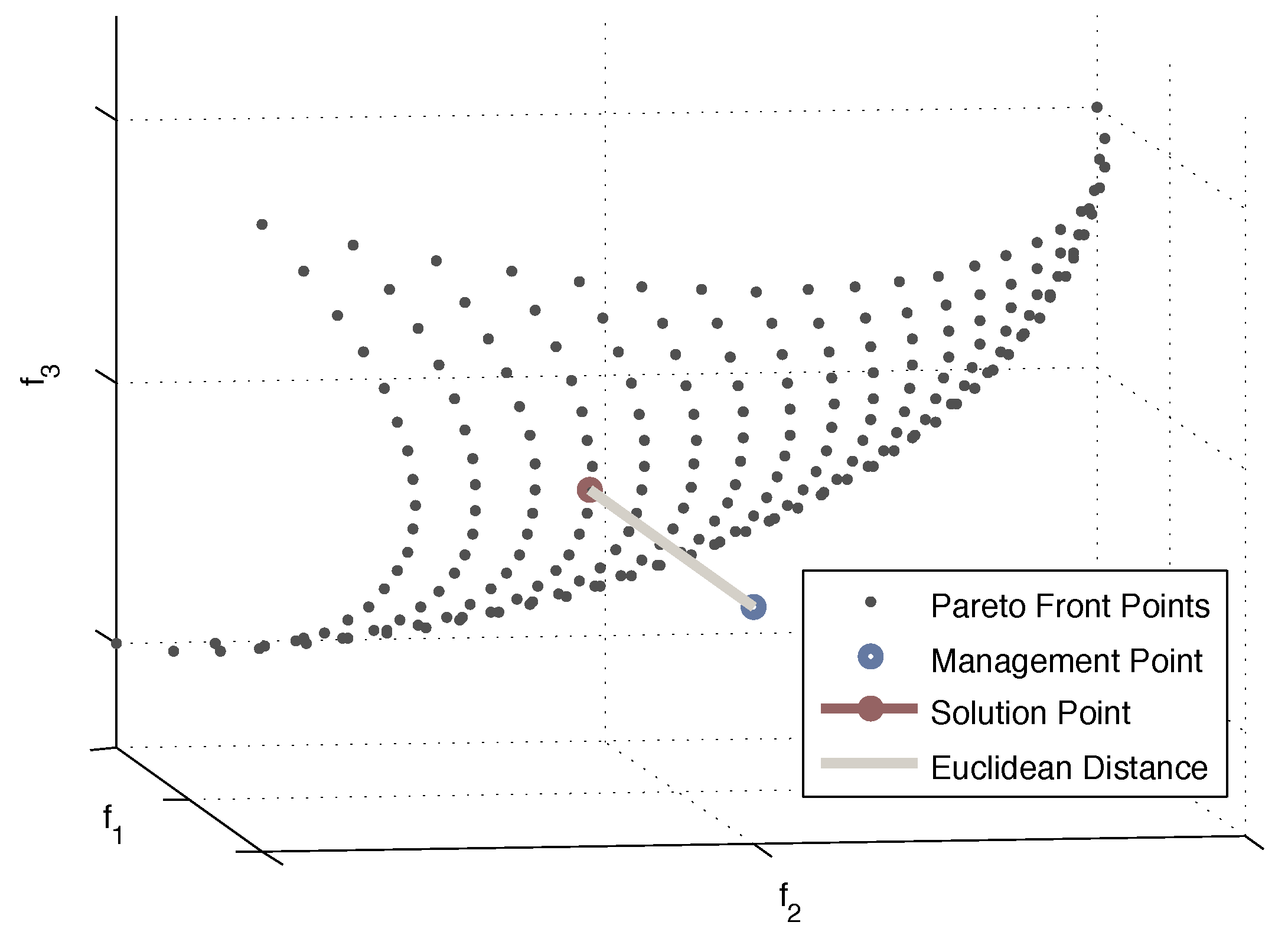
In this section, a DM strategy, based on the minimum distance to a point over the normalized design space, is proposed. The main idea is to define this management point (MP) and calculate the minimum Euclidean distance from the MP and the solutions of the Pareto front. The selected solution is calculated as

$$F_{MP}=\arg (\min \parallel {\overline{F}}^i-MP{\parallel }_2),i=1\dots n_f,$$

(15)

where ${\overline{F}}^i$ is the i-th point of the obtained Pareto front, and $MP$ is the Management Point.

4.1.2. DM Procedure and Prioritization

In order to establish a prioritization scheme, an MP based on prioritization percentages (PP) is defined as

$$MP={[M{P}_{1}M{P}_2\dots M{P}_{n_f}]}^{\top },$$

(16)

where $M{P}_i$ is the i-th coordinate of the MP, defined as:

$$\frac{(100-P{P}_i){\overline{F}}_i^N}{100},$$

(17)

being $P{P}_i$ the priority percentage of the objective function i (100 is the maximum priority percentage), defined by the user as $PP=[P{P}_{1}P{P}_2\dots P{P}_{nf}]$, and ${\overline{F}}_i^N$ is the i-th normalized nadir point. In Figure 1, a graphical explanation of the DM algorithm is presented. The applied control action corresponds to the solution point, which is the one who has the minimum distance to the management point defined previously.

Remark 1.

The introduced DM strategy uses a posteriori articulation of preferences since a solution point is selected after the calculation of Pareto-front points (see [30]).

Remark 2.

If this DM strategy is used in an online implementation, the calculation time must be taken into account because the computational burden of calculating the Pareto front at each sample time may be (too) high.

4.2. Tuning Strategy Proposals

In this section, two tuning strategies are presented. They are based on the previously derived decision-making procedure. The aim is to avoid the online computation of the Pareto front at each MPC iteration, while enabling that the selection of controller weights can still be performed based on an accurate representation of the Pareto set. Hence, the tuning is split up in an offline training phase and an online application phase. During the training phase, Pareto fronts are computed for a number of different scenarios with different disturbances (water demands). Each time, the preferred solution is also selected based on the decision-making procedure. Two approaches are evaluated for selecting the final weights for the online application: either the weights occurring most often in the corresponding histogram of preferred weight sets are selected (see Histogram-Based Weights Selection below), or a model is built to relate the preferred controller weights to the average water demands d (see Model-Based Weights Selection below).

4.2.1. Histogram-Based Weights Selection

The idea behind the histogram-based weighting is to select the set of weights which yields most often a desired solution as found by the decision-making procedure in the training phase. In general, such a procedure consists of the following steps:

• Step 1. Calculate the number of water-demand combinations for the Pareto front for the specified objective functions.
• Step 2. Select, for all Pareto fronts, the preferred solution according to the decision-making procedure described above.
• Step 3. Make a histogram of the occurrence of the different sets of selected weights for the Normalized Weighted Sum.
• Step 4. Select, in the histogram, the weights with the highest number of occurrences and use the weights for implementation in the MPC.
• Step 5. Evaluate the controller in an online setting (without computing the entire Pareto set in each iteration).

This strategy can be used as a starting point for an empirical tuning of MPC weights.

4.2.2. Model-Based Weights Selection

In this case, not a single set of weights is adopted but the weights for the MPC are calculated dynamically on the basis of the average water demands. To be able to do so, a regression model is needed. This leads to the following general procedure:

• Steps 1 to 3 are identical to the previous approach.
• Step 4. Calculate a regression model of the preferred set of weights as a function of the average of water demands.
• Step 5. Evaluate the controller in an online setting, i.e., in each MPC, use the regression model for the calculation of weights based on the water demand.

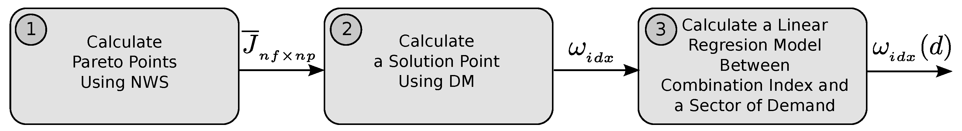
Figure 2 shows a flowchart of the proposed tuning strategy process. The output data of the second process are represented by ${\omega }_{idx}$, which is the weighting combination index, defined as the column of matrix W, that corresponds to the weighting combination used in the solution point, ${\overline{J}}^{\ast }$. It has been seen that there is a relation between ${\omega }_{idx}$ and the average demand, $\tilde{d}$, hence, a linear regression model can be calculated in order to modify the weighting factors in function of the variations of $\tilde{d}$, i.e.,

$${\omega }_{idx}=f\left(\tilde{d}\right),$$

(18)

where $f:\mathbb{R}\to \mathbb{Z}$ and $\tilde{d}\in \mathbb{R}$.

Remark 3.

The use of any of the Pareto front calculation methods and the proposed DM strategy constitutes an implicit MPC-tuning strategy.

5. Application Example

The case study considered in this paper has been previously presented in the literature of the predictive control of large-scale systems [7,31]. In these references, details concerning the control-oriented modelling and management criteria of the Barcelona DWTN are explained and discussed in detail. In this paper, and for completeness, the most important elements are highlighted.

5.1. Aggregate Model of the Barcelona DWTN

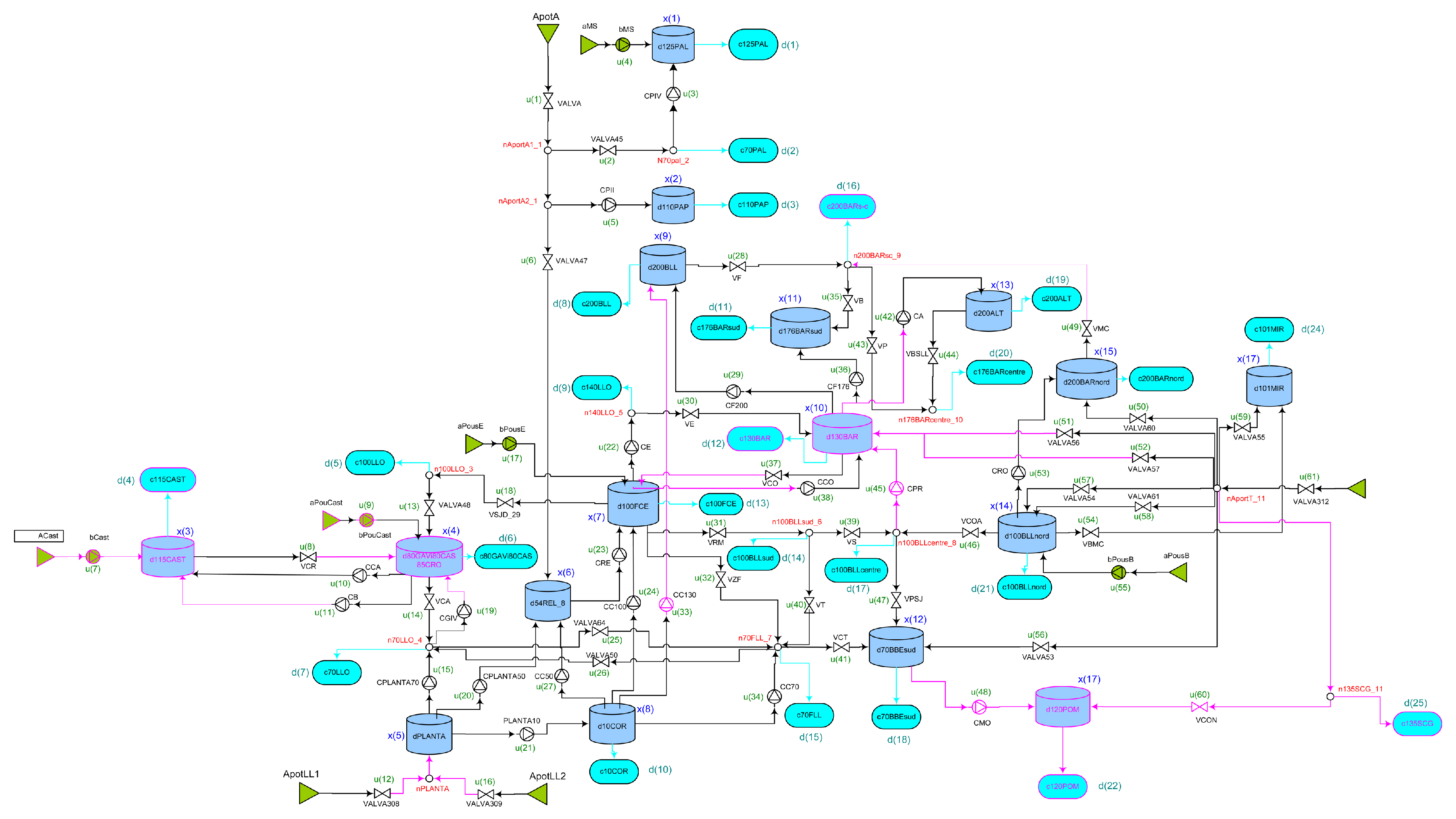
The Barcelona DWTN covers a territorial extension of 425 km${}^2$, with a total pipe length of 4470 km. Every year, it supplies 237.7 hm${}^3$ of drinking water to a population of over 2.8 millions of inhabitants. The main sources of water are the Ter and Llobregat rivers, which are regulated at their head by some dams with an overall capacity of 600 hm${}^3$. Currently, there are four drinking water treatment plants (WTP): the Abrera and Sant Joan Despí plants, which extract water from the Llobregat river; the Cardedeu plant, which extracts water from the Ter river; and the Besòs plant, which treats the underground flows from the aquifer of the Besòs river. There are also several underground sources (wells) that can provide water through pumping stations. Those different water sources currently provide a flow of around 7 m${}^3$/s. The most important sources in terms of capacity are the Sant Joan Despí and Cardedeu plants. The maximum flow that can be taken from the first is about 5 m${}^3$/s, while the maximum flow from the second is about 7 m${}^3$/s. The water price from each source is different depending on water treatments and legal extraction canons [7].

The network has a centralized telecontrol system, organized in a two-level architecture. At the upper level, a supervisory control system installed in the control center of AGBAR (AGBAR: Aguas de Barcelona, S.A. is the company that manages the DWTN of Barcelona city and its metropolitan area) is in charge of managing the whole network by taking into account operational constraints and consumer demands. This upper level provides the set-points for the lower-level control system. The lower level optimizes the pressure profile to minimize losses due to leakage and to provide sufficient water pressure, e.g., for high-rise buildings. This paper considers an aggregate version of the Barcelona DWTN, shown in Figure 3, which is a representative version of the entire network presented in [7]. In the aggregate model, some water demand sectors are grouped in a single one with the same total water demand. Similarly, some tanks are aggregated in a virtual single tank with the volume equal to the sum of the individual volumes and the respective actuators are considered as a single pumping station or valve. In

Table 1. Components of the aggregate model.

Type of Component	Quantity
Water storing tanks	17
Pumping stations	26
Valves	35
Nodes	11
Sectors of consume	25

, a brief summary of the aggregate model is presented. The global behavior of such a model is similar to the one of the complete network.

In the following section, simulation results are presented and discussed. The Pareto front calculation methods introduced in Section 3 have been used to generate the Pareto set of the MOO problems related to the case study and to illustrate its varying nature. The proposed decision-making strategy has been evaluated using two Pareto front calculation methods and key performance indicators (KPIs) that were introduced in order to compare the obtained results. At the end of the section, a regression model obtained to test the proposed tuning strategy is presented. Finally, a comparison between the results obtained by using the tuning strategies is presented in Section 4.2, and two MPC implementations with fixed weighting factors are discussed.

5.2. Pareto Front Generation for the DWTN Problem

The interesting feature about obtaining the Pareto front in this MPC problem is that, at each iteration, the front changes as a function of the disturbances.

In order to calculate the Pareto front points, two solvers have been used. For the methods involved with normal constraints (NNC and ENNC), anchor points have been calculated using the TOMLAB/CPLEX solver, and, for the calculation front points (the case of ENNCP), the TOMLAB/SNOPT solver has been deployed. As has been exposed previously, the NWS optimization problems are convex, hence, in order to calculate Pareto front points with this method, only the TOMLAB/CPLEX solver has been used.

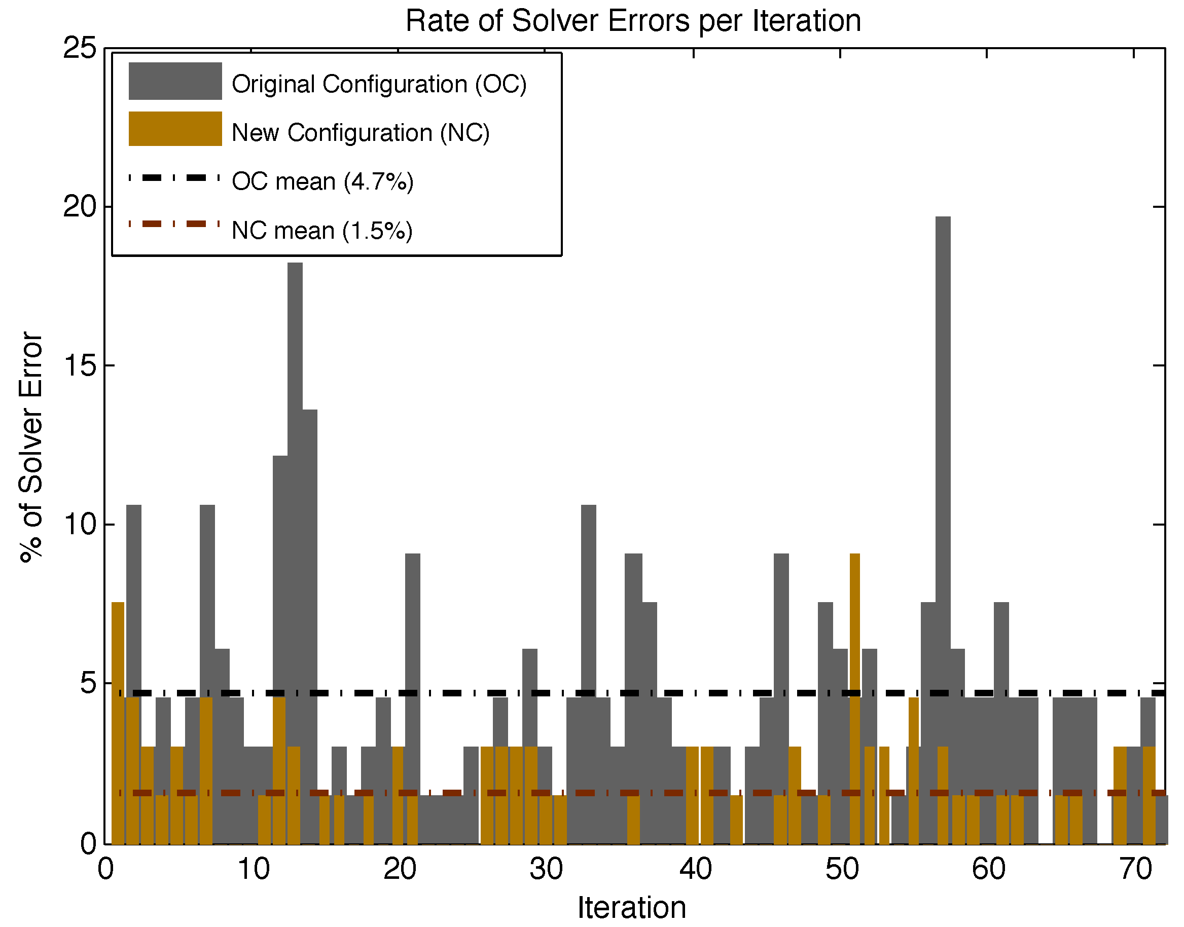
5.3. Solver Errors

Mainly, due to the non-linear characteristic of the (E)NNC sub-problems, three types of optimization errors have been observed

• Infeasibility problem errors;
• Resource limit errors, related to the maximum number of iterations; and
• Numerical errors, related to ill-conditioning issues.

The error rate, defined as $100(n_e/n_p)$ (where $n_e$ is the number of solver errors and $n_p$ is the number of Pareto-front points), has been collected in the simulation in order to check it and define some corrective configurations, such as, increase the maximum iteration number, choose a knowledge-based starting point and activate the problem-scaling option. In Figure 4, the error-rate evolution over time is presented, and a comparison between the solver error rate before and after the corrective configurations.

Remark 4.

For the non-linear solver, each corrective configuration implies a longer calculation time.

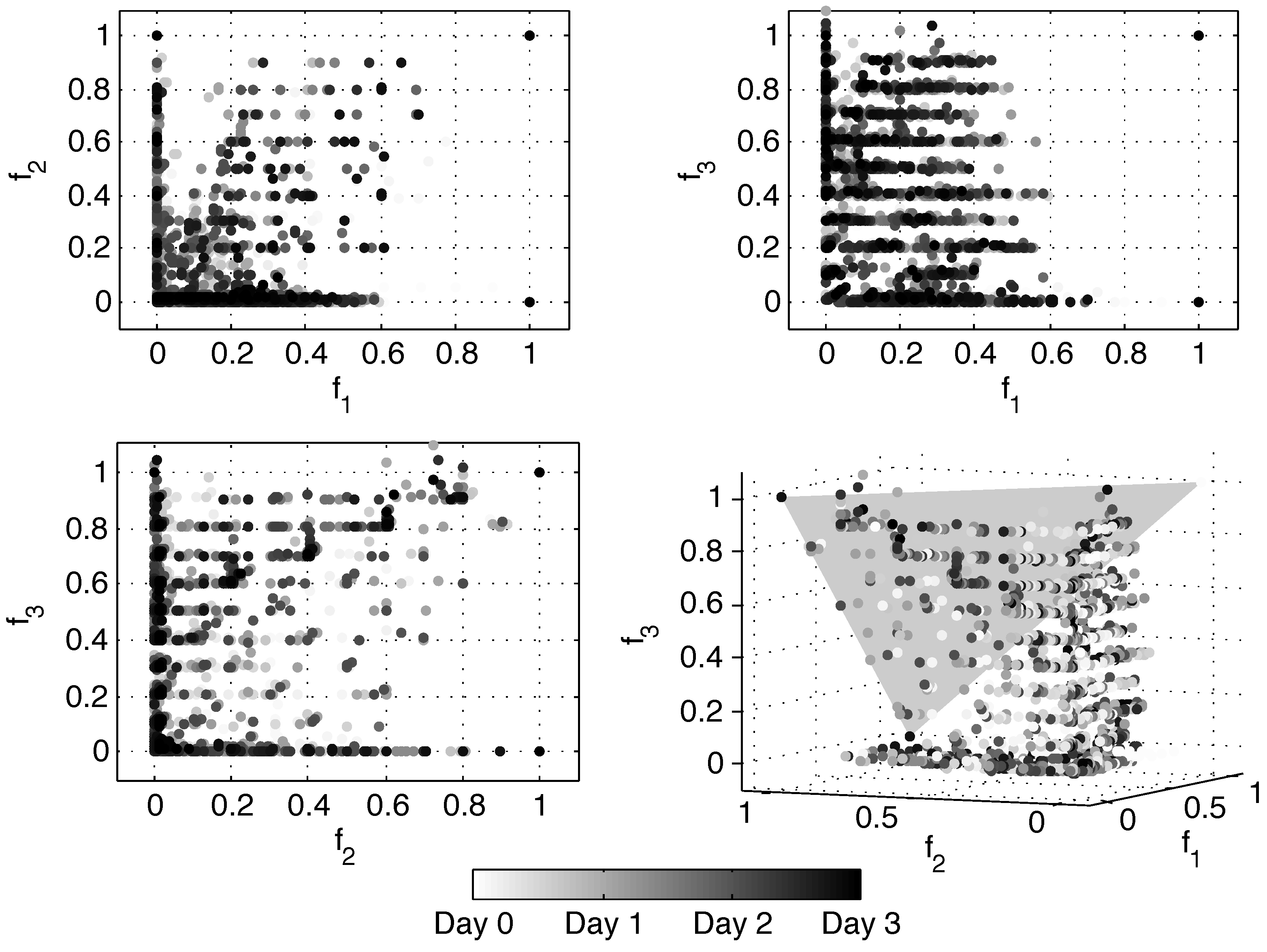
Regarding the Pareto-front calculation with ENNCP and to illustrate the evolution of the Pareto front over time, Figure 5 shows the obtained points, with different perspectives, for a 72 h simulation. The utopia plane has been drawn in light-gray color along with the 3D plots in order to show the whole design space. It is also clear that the Pareto set is compatible with the proposed DM algorithm.

5.4. Key Performance Indicators

To compare the results obtained from the different tuning strategies, the KPIs presented next have been defined based on the DWTN objective functions introduced in Section 2.2.

Economic KPI: This performance indicator is related to the water production and transport costs (4), and is defined as

$$KP{I}_{\mathrm{cost}}=\frac{\Delta t}{N}\sum _{k=1}^N({\alpha }_1+{\alpha }_2\left(k\right))u\left(k\right),$$

(19)

where N is the number of samples considered in the evaluation (length of the simulation scenario).

Safety KPI: This performance indicator is related to the volume-regulation strategy of the tanks. It has been defined as

$$KP{I}_{\mathrm{safety}}=\frac{1}{N}\sum _{k=1}^N\epsilon \left(k\right),$$

(20)

where $\epsilon \left(k\right)$ denotes the amount of the safety volume constraint violation at time k.

Smoothness KPI: This performance indicator is related to the smoothness of the control movements, and is defined as

$$KP{I}_{\mathrm{smoothness}}=\frac{1}{(N-1)}\sum _{k=2}^N{(\Delta u\left(k\right))}^2,$$

(21)

where $\Delta u\left(k\right)$ is the incremental control movement applied at time k.

Remark 5.

A reduction in the KPI values implies a better performance of the designed closed-loop control scheme based on an EMP controller tuned by using the proposed approaches.

5.5. DM Strategy Simulations

Using the DM strategy stated in Section 4.1, six simulations have been performed considering different Pareto front calculation methods and management point definitions using the normalization with pseudo-anchor points. The results are presented, taking into account that the nominal performance is achieved from the second day of simulation. The selected baseline performance is the one with the best trade-off between the objectives, i.e., MP = [0, 0, 0]${}^{\top }$ (obtained from PP = [100, 100, 100]${}^{\top }$).

5.5.1. DM Exploiting ENNCP

The obtained results are presented in

Table 2. KPIs for the DM Strategy using the ENNCP Method.

Priority Percentages	Economic KPI		Safety KPI		Smoothness KPI
	Day 2	Day 3	Day 2	Day 3	Day 2	Day 3
[100 100 100]	34.3553	33.7995	3873.5	3888.2	0.0040	0.0042
[100 75 50]	34.0348	33.5804	3900.5	3878.1	0.1699	0.1549
[50 100 75]	39.6096	38.9024	4195.9	3931.9	0.0495	0.0538
[75 50 100]	38.1425	36.4246	3716.1	3678.3	0.0019	0.0006

. The idea behind the definition of priority percentages is to establish a tuning approach from the DM algorithm point of view, more specifically, a prioritization procedure. Results obtained with PP = [100, 75, 50]${}^{\top }$ show that the prioritization of the economic objective $J_1$ over the rest has been achieved, and is reflected by the reduction in the economic KPI with respect to the baseline. In the results obtained with PP = [50, 100, 75]${}^{\top }$, where $J_2$ was mainly prioritized, the defined MP carried out the control problem to a zone where the management criteria was affected negatively, leading to a notable increase in the KPIs in comparison with the baseline. Finally, results obtained with PP = [75, 50, 100]${}^{\top }$ show a clear reduction in the variability of control actions, hence, an increase in the other two KPIs.

Taking advantage of the DM scheme, results adding the constraint

$$\sum _{i=1}^{n_f}P{P}_i=100$$

(22)

are also presented. The idea of the equality constraint (22) is to establish a clearly prioritized selection of the solution point.

The obtained results are presented in

Table 3. KPIs for the DM Strategy (with condition (22)) using the ENNCP Method.

Priority Percentages	Economic KPI		Safety KPI		Smoothness KPI
	Day 2	Day 3	Day 2	Day 3	Day 2	Day 3
[100 100 100]	34.3553	33.7995	3873.5	3888.2	0.0040	0.0042
[50 30 20]	34.4205	33.7557	4853.6	4541.7	0.2184	0.2632
[20 50 30]	49.6496	48.7163	3360.7	3359.5	0.0186	0.0034
[30 20 50]	46.9891	43.6090	3658.0	2537.8	0.0003	0.0002

. Note that the use of condition (22) clearly establishes the prioritization of the objective with the larger PP—in some cases, it has even been seen that the prioritization was extreme and the selected solution was one of the anchor points, in which the prioritized objective had its minimum cost but the others, sometimes, had their worst value.

5.5.2. DM Exploiting NWS

In order to compare different approaches, the DM strategy has also been tested using the NWS method. Results are presented in

Table 4. KPIs for the DM Strategy using the NWS Method.

Priority Percentages	Economic KPI		Safety KPI		Smoothness KPI
	Day 2	Day 3	Day 2	Day 3	Day 2	Day 3
[100 100 100]	34.3305	33.6452	3809.5	3822.2	0.0039	0.0035
[100 75 50]	34.0022	33.4155	3501.8	3371.0	0.0086	0.0092
[50 100 75]	42.7737	42.1820	4068.1	4000.4	0.0024	0.0018
[75 50 100]	35.0110	34.2817	3578.0	3827.3	0.0028	0.0026

and

Table 5. KPIs for the DM Strategy (with condition (22)) using the NWS Method.

Priority Percentages	Economic KPI		Safety KPI		Smoothness KPI
	Day 2	Day 3	Day 2	Day 3	Day 2	Day 3
[100 100 100]	34.3305	33.6452	3809.5	3822.2	0.0039	0.0035
[50 30 20]	33.8902	33.1499	4704.4	4886.1	0.2069	0.2217
[20 50 30]	50.0738	48.7135	3309.9	3353.7	0.0032	0.0034
[30 20 50]	48.3035	49.6586	3402.5	2178.9	0.0002	0.0001

. Note that the baseline value is slightly different in this case, compared to the baseline obtained with the ENNCP method. This is among others due to the use of different solvers. As said before, in the ENNCP method, only the anchor points are calculated with CPLEX because they are convex optimization problems. The rest of the points (63 of them) are solved with SNOPT. In the case of simulations with the NWS method, all the Pareto front points have been calculated with CPLEX because all the optimization problems are convex. Again, similar results are observed.

In Table 5, results have been calculated using the condition (22). Concerning the obtained results, note that the KPIs show the same tendency as those calculated in the ENNCP simulations.

5.6. Weight Variations and Measured Disturbances

In this section, the results from the method simulations for choosing MPC weighting factors, as proposed in Section 4.2.1, are presented.

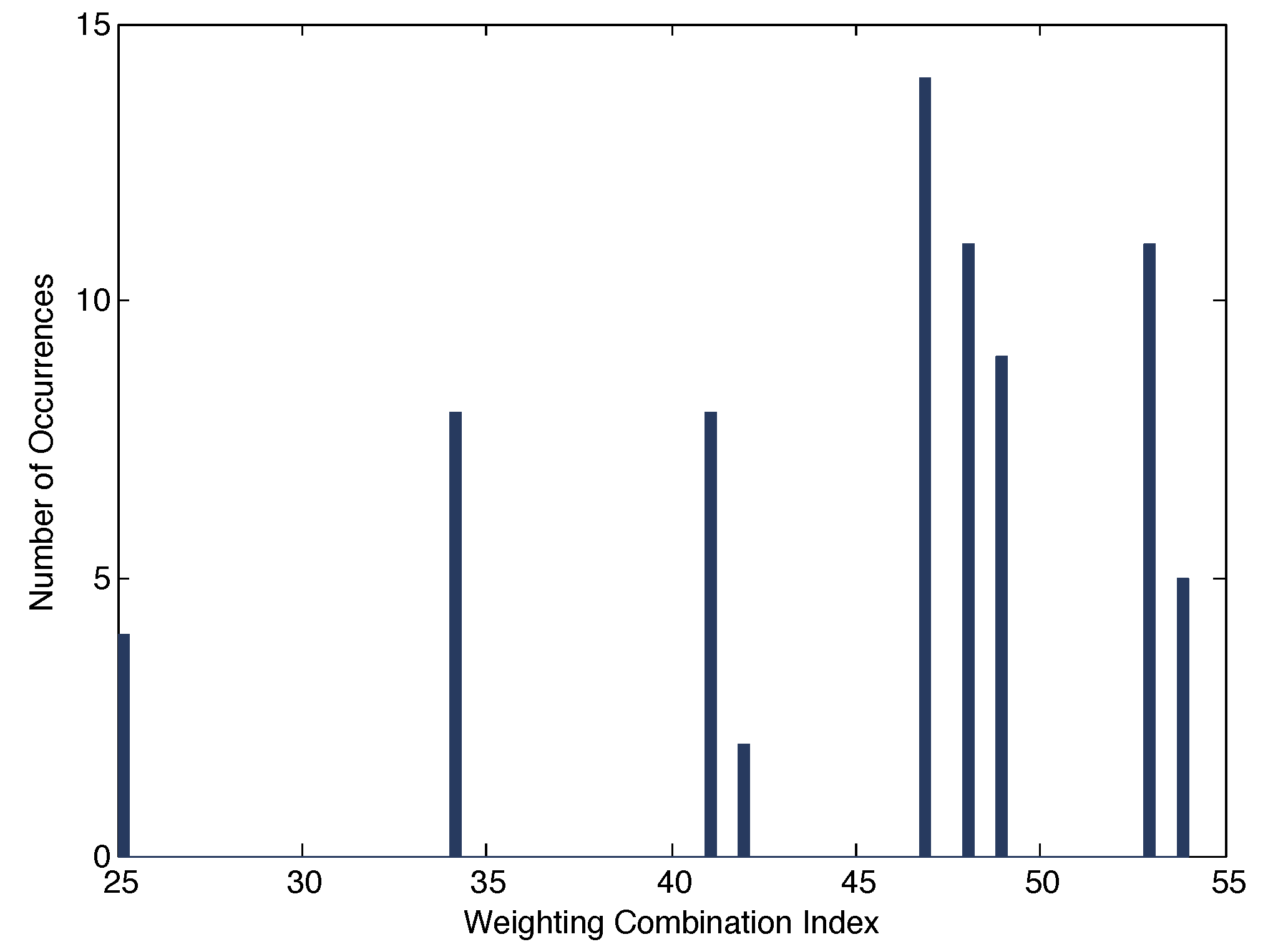
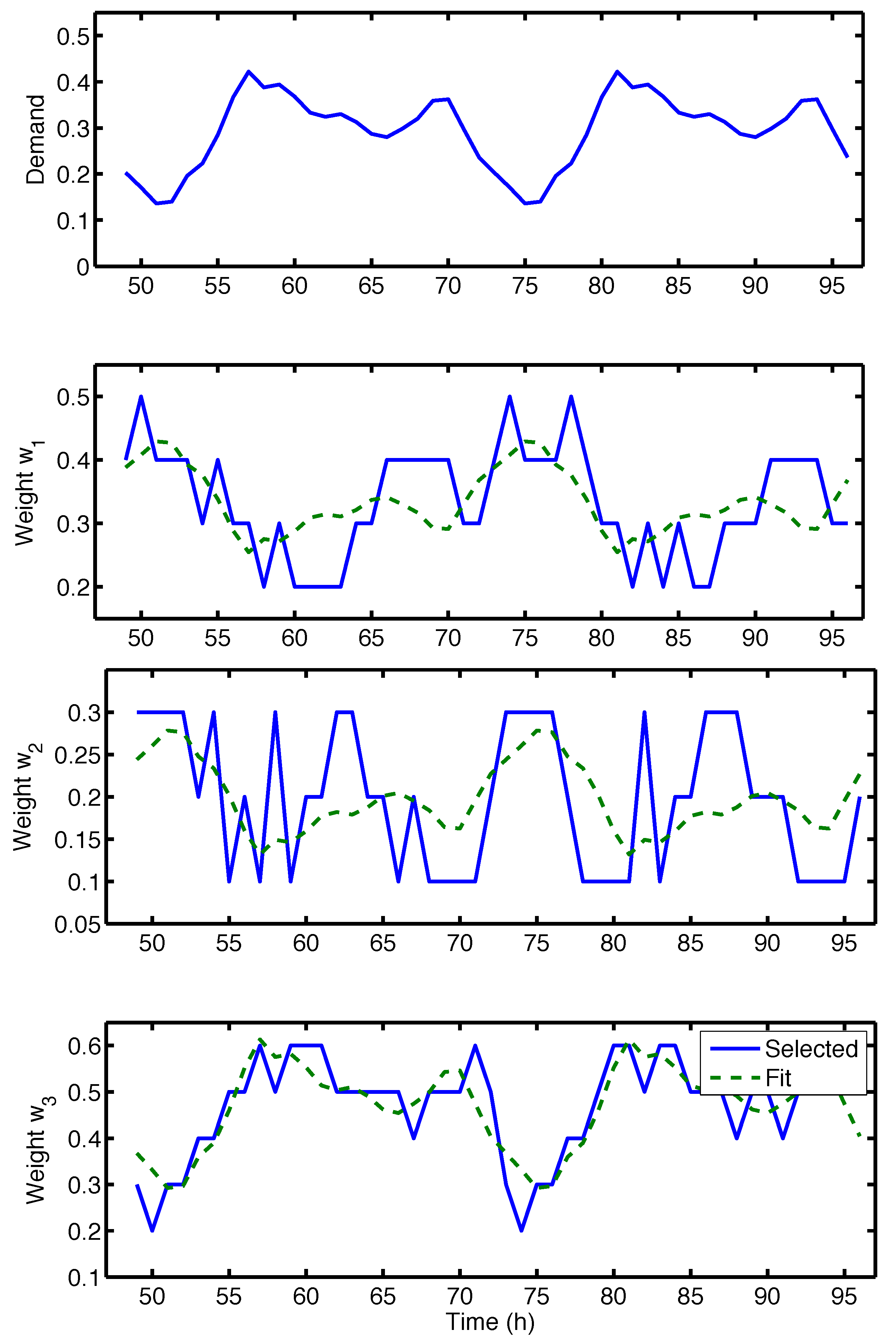
The histogram of the weight sets along a four day simulation scenario is presented in Figure 6. The most used weight combination has been ${[w_1,w_2,w_3]}^{\top }={[0.4,0.1,0.5]}^{\top }$. It has been seen that there is a relation between the adopted weight values and the average demand, $\tilde{d}$, hence, a regression model can be calculated in order to modify the weighting factors in function of the variations of $\tilde{d}$. Figure 7 shows the temporal responses of the weights, and the average demand, $\tilde{d}$, as well as a regression between the variables. The correlation index is 0.83, meaning that there is a correlation between the variables, hence, a representatively enough regression model can be calculated.

5.7. Tuning Strategy

Four tuning strategies have been compared for a centralized predictive control scheme over the aggregate model of the Barcelona DWTN. First of all, the original EMPC implementation, without normalization, is simulated. Then, an EMPC implementation with normalization of the objective functions is introduced. Finally, the tuning strategies proposed in Section 4.2 are applied. The KPIs calculated with the simulation of the first EMPC implementation have been selected as the baseline performance. The weighting factors of the first two EMPCs are ${[w_1,w_2,w_3]}^{\top }={[1/3,1/3,1/3]}^{\top }$.

5.8. Results Discussion

Table 6. Tuning Strategies Comparison.

Tuning Strategy	Economic KPI		Safety KPI		Smoothness KPI
	Day 2	Day 3	Day 2	Day 3	Day 2	Day 3
Original MPC	34.4477	34.5007	3921.7	3912.3	0.0105	0.0103
Normalised MPC	34.5643	34.6338	3837.6	3838.3	0.0026	0.0025
Histogram-Based Weighting	34.1424	34.2004	3324.7	3337.2	0.0017	0.0017
Adaptive Weighting	33.4410	33.0017	3135.9	3023.0	0.0007	0.0006

shows the obtained results for a three-day simulation, where only the key performance indicators of days 2 and 3 have been considered in order to avoid transient responses. Regarding the results, note that the two proposed EMPC-tuning strategies outperform the performance of the equally weighted EMPCs. Moreover, the EMPC with adaptive weighting combinations has shown the best performance, giving the lowest KPIs. On the other hand, although the proposed tuning approaches are here applied to a DWTN, the methodology is quite transversal and can be extrapolated to other large-scale flow-based networks with multiple control objectives. For other case studies, several details and procedures should be slightly modified but, in essence, the methodology remains quite similar (e.g., more control objectives to be tuned, more complex models of the DWTNs, among others).

Regarding the social dimension issue, the proposed approaches applied to the particular critical infrastructure considered here (the DWTN) positively affect aspects related to the reduction in economic costs from the system’s managing company, which can be reflected in lower fees for the customers since a better and closely optimal operation of the system elements (from the energy efficiency viewpoint) would rise in lower electricity consumption related to the treatment and transport of water. Aside of that, a suitable control policy would improve several resilience indicators, such as those reported by [32] (particularly related to the case study) and others reported in [33,34].

6. Conclusions and Further Work

In this paper, economic model predictive controllers have been tuned using scalarization-based multi-objective approaches. First, the dynamic nature of the underlying Pareto front has been highlighted. Second, a strategy has been proposed which enables that the preferred controller parameters reflecting the decision maker’s preferences are always adopted. The strategy involves an offline training phase and an online application phase. During the offline training phase, the controller parameters are selected for different disturbances based on the decision maker’s preferences. During the online phase, two approaches are evaluated: (i) exploiting the controller parameters with the highest frequency in the histogram with selected parameter combinations or (ii) using a regression model between the controller parameters and the disturbances. Afterwards, both approaches have been tested for a real-life simulation case study related to the model predictive control of the Barcelona drinking water network. For this case study, it has been observed that the proposed tuning strategies give rise to an improved performance compared to the baseline results. As future research, the proposed approach will be extended to the case of model uncertainty (both in network model and demands). In addition, the aim is to look for faster implicit MPC-tuning strategies by the use of goal programming techniques or by the statement of only one ENNCP sub-problem as a function of the management point. Those ideas could be investigated in order to avoid the calculation of the entire Pareto front, ensuring that the applied control actions are in line with the management criteria.

References

- Ellis, M.; Durand, H.; Christofides, P.D. A tutorial review of economic model predictive control methods. J. Process Control 2014, 24, 1156–1178. [Google Scholar] [CrossRef]
- Maciejowski, J.M. Predictive Control with Constraints; Prentice Hall: London, UK, 2002. [Google Scholar]
- Rawlings, J.; Mayne, D.; Diehl, M.M. Model Predictive Control: Theory, Computation, and Design, 2nd ed.; Nob Hill Publishing: Madison, WI, USA, 2020. [Google Scholar]
- Qin, J.; Badgwell, A. A survey of industrial model predictive control. Control Eng. Pract. 2003, 11, 733–764. [Google Scholar] [CrossRef]
- Limon, D.; Alamo, T. Tracking Model Predictive Control. In Encyclopedia of Systems and Control; Springer: London, UK, 2015; pp. 1475–1484. [Google Scholar] [CrossRef]
- Albalawi, F.; Alanqar, A.; Durand, H.; Christofides, P.D. A feedback control framework for safe and economically-optimal operation of nonlinear processes. AIChE J. 2016, 62, 2391–2409. [Google Scholar] [CrossRef]
- Ocampo-Martinez, C.; Puig, V.; Cembrano, G.; Quevedo, J. Application of Predictive Control Strategies to the Management of Complex Networks in the Urban Water Cycle [Applications of Control]. IEEE Control Syst. Mag. 2013, 33, 15–41. [Google Scholar]
- Tedesco, F.; Ocampo-Martinez, C.; Cassavola, A.; Puig, V. Centralised and Distributed Command Governor Approaches for the Operational Control of Drinking Water Networks. IEEE Trans. Syst. Man Cybern. Syst. 2018, 48, 586–595. [Google Scholar] [CrossRef] [Green Version]
- Nassourou, M.; Blesa, J.; Puig, V. Robust Economic Model Predictive Control Based on a Zonotope and Local Feedback Controller for Energy Dispatch in Smart-Grids Considering Demand Uncertainty. Energies 2020, 13, 696. [Google Scholar] [CrossRef] [Green Version]
- Sebghati, A.; Shamaghdari, S. Tube-based robust economic model predictive control with practical and relaxed stability guarantees and its application to smart grid. Int. J. Robust Nonlinear Control 2020, 30, 7533–7559. [Google Scholar] [CrossRef]
- Angeli, D.; Müller, M.A. Economic Model Predictive Control: Some Design Tools and Analysis Techniques. In Handbook of Model Predictive Control; Springer International Publishing: Berlin/Heidelberg, Germany, 2019; pp. 145–167. [Google Scholar]
- Maestre, J.; Lopez-Rodriguez, F.; Muros, F.; Ocampo-Martinez, C. A Modular Feedback for the Control of Networked Systems by Clustering: A Drinking Water Network Case Study. Processes 2021, 9, 389. [Google Scholar] [CrossRef]
- Kadam, J.V.; Marquardt, W. Integration of Economical Optimization and Control for Intentionally Transient Process Operation; Springer: Berlin/Heidelberg, Germany, 2007. [Google Scholar]
- Souza, G.D.; Odloak, D.; Zanin, A.C. Real time optimization (RTO) with model predictive control (MPC). Comput. Chem. Eng. 2010, 34, 1999–2006. [Google Scholar] [CrossRef]
- Ferramosca, A.; Rawlings, J.; Limon, D.; Camacho, E. Economic MPC for a changing economic criterion. In Proceedings of the 49th IEEE Conference on Decision and Control, Atlanta, GA, USA, 15–17 December 2010. [Google Scholar]
- Garriga, J.L.; Soroush, M. Model predictive control tuning methods: A review. Ind. Eng. Chem. Res. 2010, 49, 3505–3515. [Google Scholar] [CrossRef]
- Vallerio, M.; Van Impe, J.; Logist, F. Tuning of NMPC controllers via multi-objective optimisation. Comput. Chem. Eng. 2014, 61, 38–50. [Google Scholar] [CrossRef] [Green Version]
- Wojszniz, W.; Mehta, A.; Wojszniz, P.; Thiele, D.; Blevins, T. Multi-objective optimization for model predictive control. ISA Trans. 2007, 46, 351–361. [Google Scholar] [CrossRef] [PubMed]
- Van der Lee, J.H.; Svrcek, W.; Young, B. A tuning algorithm for model predictive controllers based on genetic algorithms and fuzzy decision making. ISA Trans. 2008, 47, 53–59. [Google Scholar] [CrossRef] [PubMed]
- Alhajeri, M.; Soroush, M. Tuning Guidelines for Model-Predictive Control. Ind. Eng. Chem. Res. 2020, 59, 4177–4191. [Google Scholar] [CrossRef]
- Zavala, V.; Flores-Tlacuahuac, A. Stability of multi objective predictive control: A utopia-tracking approach. Automatica 2012, 48, 2627–2632. [Google Scholar] [CrossRef]
- Floures-Tlacuahuac, A.; Morales, P.; Rivera-Toledo, M. Multiobjective Non linear Model Preductive Ccontrol of a Class of Chemical Reactors. Ind. Eng. Chem. Res. 2012, 51, 5891–5899. [Google Scholar] [CrossRef]
- Barreiro-Gomez, J.; Ocampo-Martinez, C.; Quijano, N. Dynamical Tuning for Multi-objective Model Predictive Control based on Population Games. ISA Trans. 2017, 69, 175–186. [Google Scholar] [CrossRef] [Green Version]
- De Schutter, J.; Zanon, M.; Diehl, M. TuneMPC—A Tool for Economic Tuning of Tracking (N)MPC Problems. IEEE Control Syst. Lett. 2020, 4, 910–915. [Google Scholar] [CrossRef]
- Brdys, M.; Ulanicki, B. Operational Control of Water Systems: Structures, Algorithms and Applications. Automatica 1996, 32, 1619–1620. [Google Scholar]
- Puig, V.; Ocampo-Martinez, C.; Pérez, R.; Cembrano, G.; Quevedo, J.; Escobet, T. Real-Time Monitoring and Operational Control of Drinking-Water Systems; Springer: Berlin/Heidelberg, Germany, 2017. [Google Scholar]
- Miettinen, K.M. Nonlinear multiobjective optimization. In International Series in Operations Research & Management Science; Kluwer Academic Publishers: Boston, MA, USA, 1999; Volume 12. [Google Scholar]
- Sanchis, J.; Martinez, M.; Blasco, X.; Salcedo, J.V. A new perspective on multiobjective optimization by enhanced normalized normal constraint method. Struct. Multidiscip. Optim. 2008, 36, 537–546. [Google Scholar] [CrossRef]
- Logist, F.; Van Impe, J. Novel insights for multi-objective optimisation in engineering using Normal Boundary Intersection and (Enhanced) Normalised Normal Constraint. Struct. Multidiscip. Optim. 2012, 45, 417–431. [Google Scholar] [CrossRef]
- Marler, R.T.; Arora, J.S. The weighted sum method for multi-objective optimization: New insights. Struct. Multidiscip. Optim. 2010, 41, 853–862. [Google Scholar] [CrossRef]
- Ocampo-Martinez, C.; Puig, V.; Cembrano, G.; Creus, R.; Minoves, M. Improving water management efficiency by using optimization-based control strategies: The Barcelona case study. Water Sci. Technol. Water Supply 2009, 9, 565–575. [Google Scholar] [CrossRef]
- Robles, D.; Puig, V.; Ocampo-Martinez, C.; Garza, L. Reliable Fault-Tolerant Model Predictive Control of Drinking Water Transport Networks. Control Eng. Pract. 2016, 55, 197–211. [Google Scholar] [CrossRef] [Green Version]
- Hosseini, S.; Barker, K.; Ramirez-Marquez, J.E. A review of definitions and measures of system resilience. Reliab. Eng. Syst. Saf. 2016, 145, 47–61. [Google Scholar] [CrossRef]
- Pietrucha-Urbanik, K.; Studziński, A. Qualitative analysis of the failure risk of water pipes in terms of water supply safety. Eng. Fail. Anal. 2019, 95, 371–378. [Google Scholar] [CrossRef]
Figure 1.
DM strategy graphically explained.
Figure 2.
Tuning Strategy Flowchart.
Figure 3.
Aggregate case of the Barcelona Drinking Water Network.
Figure 4.
Rate of Solver Errors for the ENNC.
Figure 5.
Pareto front over the normalized design space calculated with the ENNCP method.
Figure 6.
Histogram of solution index.
Figure 7.
Disturbances, selected weights and regression models.