Is It Possible to Reduce Agricultural Carbon Emissions through More Efficient Irrigation: Empirical Evidence from China

Abstract

Although irrigation systems are critical to the long-term viability of agriculture, they also contribute a significant amount of carbon dioxide emissions. This creates a conflict between reducing greenhouse gas emissions and promoting agricultural growth. Researchers may be able to gain a better understanding of the subject by looking at the connection between irrigation water efficiency (IWE) and agricultural carbon emissions (ACE). With data from 30 Chinese provinces collected between 2002 and 2019, this study examines the dynamic effect of IWE on ACE. According to the results, IWE has the potential to significantly raise ACE. The positive effects of IWE become more pronounced as ACE increases, according to the heterogeneity analysis. ACE in northern China is also more vulnerable to IWE than other ACE regions. Irrigation scales appear to be a significant channel through which IWE positively affects ACE, according to an investigation of possible mechanisms. However, the increased IWE causes the planting structure adjustments, which aids in the reduction of ACE. The results of this study have significant ramifications for public policy.

1. Introduction

It has been decades since China’s economy has achieved such great and exceptional milestones thanks to its reform and opening-up program, which began in 1978. Over the last four decades (i.e., 1978–2020), China’s total GDP has grown 276 times, from 367.9 billion yuan to 101,598.6 billion yuan, with an average annual growth rate of 13.96 percent, according to the China Statistical Yearbook. Environmental concerns, most notably CO₂ emissions, have become increasingly crucial as China’s economy booms. [1,2]. China released about 1418.5 million tonnes (Mt) of CO₂ in 1978 and 9825.8 Mt in 2019, an almost sevenfold increase [1]. President Xi Jinping declared in September 2020 that China’s goal is to peak carbon emissions by 2030 and achieve carbon neutrality by 2060. This brilliant aim, which has the potential to considerably decrease global warming, raises concerns about the goals’ practicality. Agriculture accounts for 17 percent of total greenhouse gas emissions in China, but just 7 percent in the United States and 11 percent globally. [3]. As a result, China will benefit more from lowering agricultural carbon emissions (ACE) than other nations.

As a big country with a large population and an even larger economy, guaranteeing food security and sustainable agricultural development is critical for China’s stability and prosperity. Irrigation is critical for agricultural output to be successful. China’s water scarcity significantly jeopardizes agricultural productivity and is a significant constraint on the country’s development. As climate change progresses and droughts worsen, guaranteeing irrigation is a critical component of climate change mitigation [4,5]. Therefore, increasing agricultural water efficiency is a critical national strategy and a subject of continuing research by a large number of experts [6,7]. Improving water efficiency means using less water to achieve the same goal, which means less water is wasted, which helps combat water scarcity. Improving irrigation water efficiency (IWE) necessitates irrigation infrastructure, and agricultural irrigation is also an energy-intensive activity that generates significant volumes of greenhouse gases [8,9,10]. Because China’s agriculture relies so heavily on groundwater pumping irrigation, this problem is particularly acute in China. Groundwater pumping in irrigation systems alone accounts for 40% of overall agricultural carbon emissions in China [11]. This creates a paradox: irrigation is important for agricultural sustainability and adaptation to climate-change-related events such as drought, while agricultural carbon emissions from irrigation contradict China’s carbon reduction ambitions.

Some scholars believe that the importance of improving irrigation water efficiency is not only to ensure the use and supply of water, but also to reduce unnecessary waste and energy input for irrigation, thus reducing greenhouse gas emissions from irrigation systems [10,12]. However, it has been maintained that there is an irrigation paradox [13]. Increased irrigation efficiency results in increased water consumption. Increased irrigation efficiency allows for the cultivation of more water-intensive crops, the expansion of irrigated areas, and the expansion of irrigation facilities. If this is the case, increasing irrigation efficiency will not result in water and energy savings, but will instead result in an increase in carbon emissions. It remains unknown, then, how improving irrigation water use efficiency actually affects agricultural carbon emissions, a research question that has important implications but has received little attention and lacks direct evidence to investigate the relationship.

Numerous research on irrigation energy consumption and carbon emissions have been conducted, it is mainly examined from the perspective of a single energy input dimension [14,15,16,17,18,19]. As a result, it is difficult to draw any conclusions on the connection between IWE and ACE from this research. In addition, actual agricultural production is situated in a specific social context, for example, the national context of agricultural production in China is still dominated by decentralized smallholder farmers [20]. Because agricultural production inputs are frequently substitutable, selecting a comprehensive IWE indicator is critical for a better understanding of the IWE–ACE link. These issues are not addressed and considered in existing studies. In other words, researching the effect of IWE on ACE in China—the world’s largest developing country—is more typical and can serve as a model for other countries facing water scarcity and a strong desire to reduce carbon emissions.

In light of the aforementioned knowledge shortages, this study first quantifies the IWE indicators using data envelopment analysis (DEA), and then examines the dynamic impact of IWE on ACE in China using panel data from 30 Chinese provinces from 2002 to 2019. Additionally, this study examines the mediation impact of IWE on ACE. Thus, our work contributes to the present body of knowledge in three ways. To begin, this study examined the IWE–ACE nexus by measuring IWE using the DEA method and obtaining ACE data from the China Emission Accounts and Datasets (CAEDs) [21,22,23,24]. This not only clarifies how IWE affects ACE, but also assists the government in developing specific and reasonable carbon mitigation policies from an IWE perspective. Second, this work focuses on the IWE–ACE relationship’s asymmetric and heterogeneous analysis. This is critical for effectively reducing China’s CO₂ emissions by taking regional variances into account. Third, this research also explores the mediating role of numerous crucial variables (such as irrigation sizes and planting structure adjustments) in altering the IWE–ACE nexus, which can benefit local governments in understanding the specific pathways by which IWE influences ACE.

2. Materials and Methods

2.1. Data Sources

The research period is limited to 2002–2019 because of data availability. The data utilized in this study are totally collected from public database, which includes the China Statistical Yearbook, the China Rural Statistical Yearbook, the China Agriculture Yearbook, the China Agricultural Machinery Industry Yearbook.

2.2. Agricultural Carbon Emissions

Nowadays, agricultural activities are defined by a variety of carbon-based procedures and inputs. The ACE in China is calculated by taking into account a wide range of carbon emissions from a variety of sources. Mechanized agricultural operations such as tilling, planting, and harvesting are among the many uses for diesel oil. [25] Tillage alters the soil structure by removing carbon and releasing it into the atmosphere as carbon dioxide. Other sources, such as fertilizers, chemical pesticides, and agricultural film, also contribute significantly to carbon emissions due to their use as critical inputs in agricultural output. The process of manufacturing, processing, and storing these ingredients requires the combustion of fossil fuels. Carbon emissions from various agricultural operations and inputs are typically assessed in kilograms of carbon equivalent. The units of carbon emissions in this study are expressed in Mt, i.e., million tons.

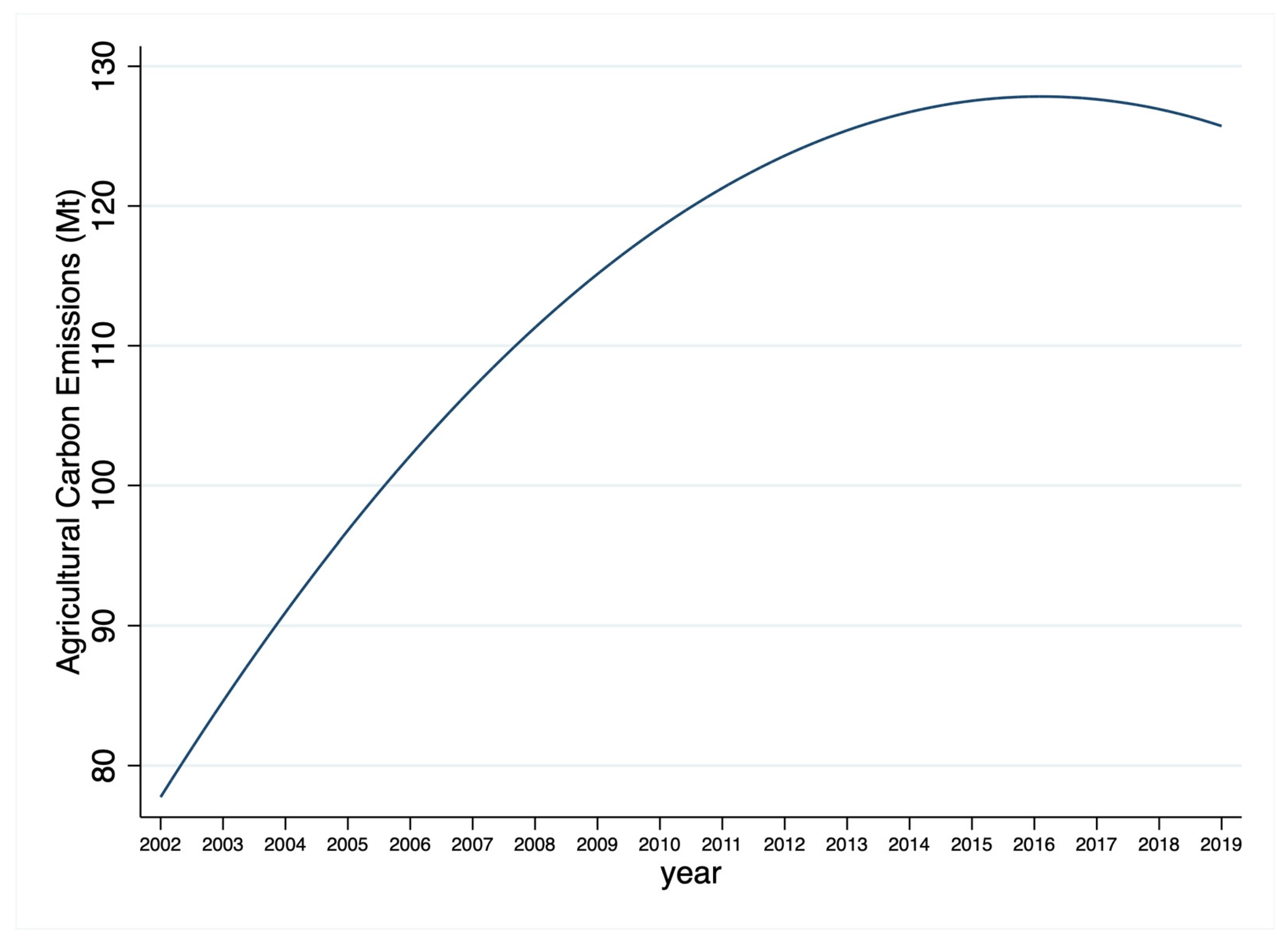
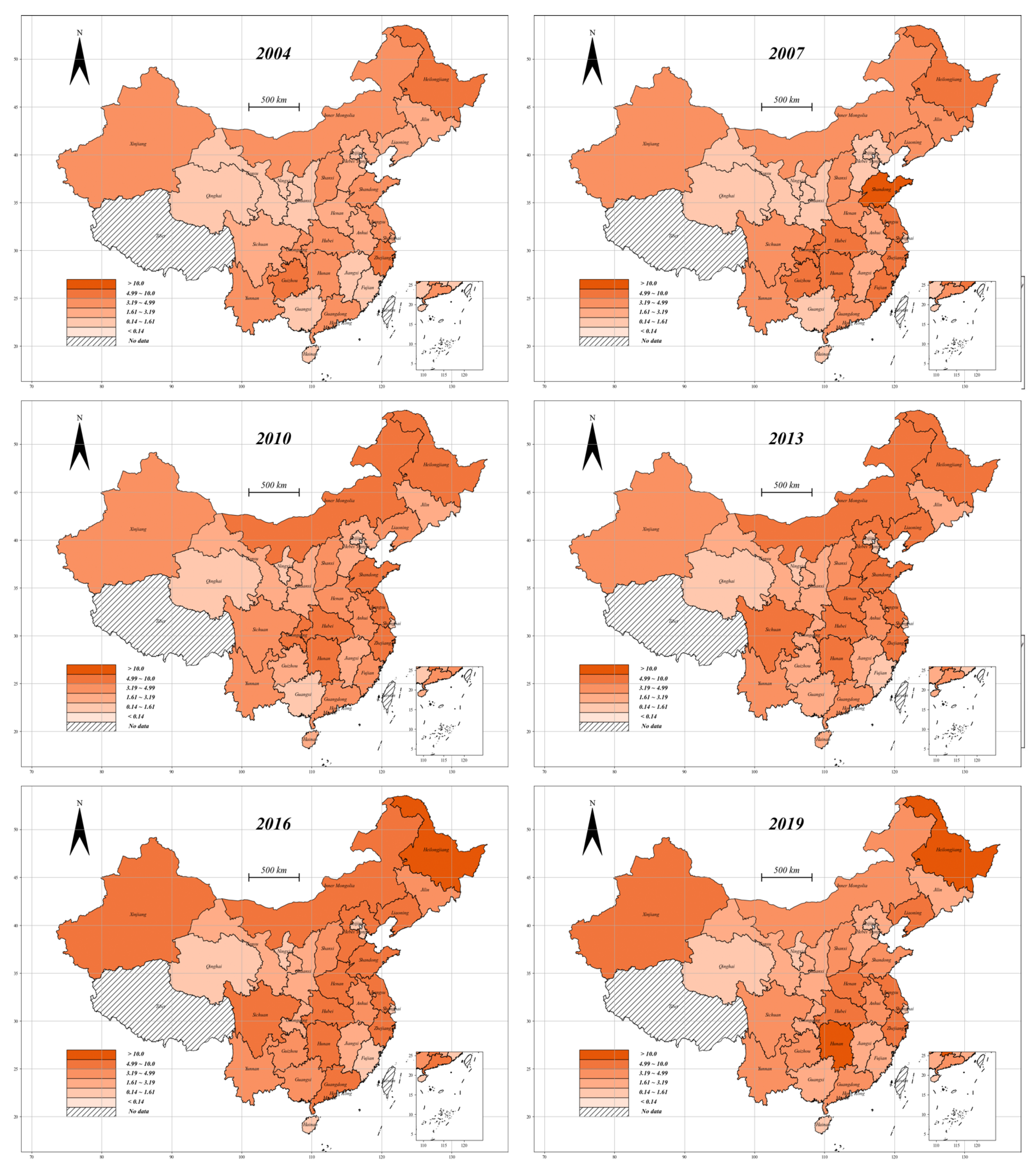
The Carbon Emission Accounts and Datasets (CEADs) contains statistics on agricultural carbon emissions in China. CEADs provide updated CO₂ emission inventories for China and its 30 provinces and municipalities on a regular basis, utilizing the IPCC’s methodology for sub-sectoral emission accounting (45 production sectors and 2 residential sectors). The IPCC Sectoral Approach calculates CO₂ emissions based on energy consumption and emission coefficients. [21,22,23,24]. In addition to the annual time series chart of ACE (Figure 1), this study also shows a map of the spatial distribution of ACE in 2004, 2009, 2014, and 2019 (see Figure 2).

2.3. Irrigation Water Efficiency Measure

Irrigation water efficiency (IWE) is a term that refers to an individual’s ability to achieve a defined level of output while using the fewest irrigation water inputs feasible [26]. At the moment, efficiency assessment is often performed using stochastic frontier analysis (SFA) and data envelopment analysis (DEA) [7]. With a specific production function, SFA maximize agricultural production efficiency. The essential model forms of DEA are CCR and BCC [27]. CCR assumes constant scale returns and is capable of measuring total efficiency, including scale efficiency. Under a variable pay-for-scale situation, the BCC model is used to estimate the pure technical and scale efficiency of the decision-making unit. Comprehensive efficiency is a concept that relates to a decision-making unit’s technological capabilities in terms of inputs and outputs. The IWE that is being quantified in this research is premised on low input costs; hence, the input-oriented CCR model is adopted.

To prevent mistakes due to the assumed production function, we utilized DEA to determine IWE. It is challenging to enhance parameter accuracy using standard DEA approaches since many decision-making units will be most efficient concurrently (efficiency is equal to 1). As a result, the super efficiency DEA model was used to calculate IWE, which is ideal for analyzing that the decision-making unit is 1 while simultaneously disregarding the decision-making unit. Agricultural irrigation water efficiency (IWE) is defined as the ratio of the ideal irrigation water input to the actual irrigation water input, using the following formula:

$$IW{E}_{i,t}=\frac{TW{C}_{i,t}}{IW{R}_{i,t}}$$

(1)

where $IW{E}_{i,t}$ denotes province i at time t in terms of irrigation water efficiency.

$TW{C}_{i,t}$ is the actual agricultural water input of province i at time t, $IW{R}_{i,t}$ is the optimal actual agricultural water input of province i at time t.

The DEA model is described as follows:

$$\begin{gathered} \min \left(\theta -\epsilon \left(S^{-}+S^{+}\right)\right) \\ \mathrm{s}.\mathrm{t}.\{\begin{array}{c}\begin{array}{c}{\displaystyle {\displaystyle \sum }_{\begin{array}{c}k=1\\ k\ne j\end{array}}^n}{X}_k{\lambda }_k+S^{-}=\theta X_j\\ {\displaystyle {\displaystyle \sum }_{\begin{array}{c}k=1\\ k\ne j\end{array}}^n}{Y}_k{\lambda }_k-S^{+}=Y_j\\ {\lambda }_k\ge 0, k=1, \dots , n \end{array}\\ S^{+}\ge 0, S^{-}\ge 0\end{array} \end{gathered}$$

(2)

For the k th DMU, $X_k$ is a set of inputs indicators vector, the $Y_k$ is output indicator, and $S^{-}$ and $S^{+}$ are the vector of input and output slack variables, respectively. ${\lambda }_k$ is the weight coefficient.

Equation (2) achieves the optimal solution, and when the following occur.

(1)

If $\theta =1$, $S^{-}=S^{+}=0$, then DMU achieves strong DEA efficiency;

(2)

If $\theta =1$, $S^{-}\ne 0$ or $S^{+}\ne 0$, then DMU is weak DEA efficiency;

(3)

If $\theta <1$, and $S^{-}\ne 0$, $S^{+}\ne 0$, then DMU is DEA invalid, which means that the DMU does not reach a proper ration. A higher θ value indicates higher DEA efficiency.

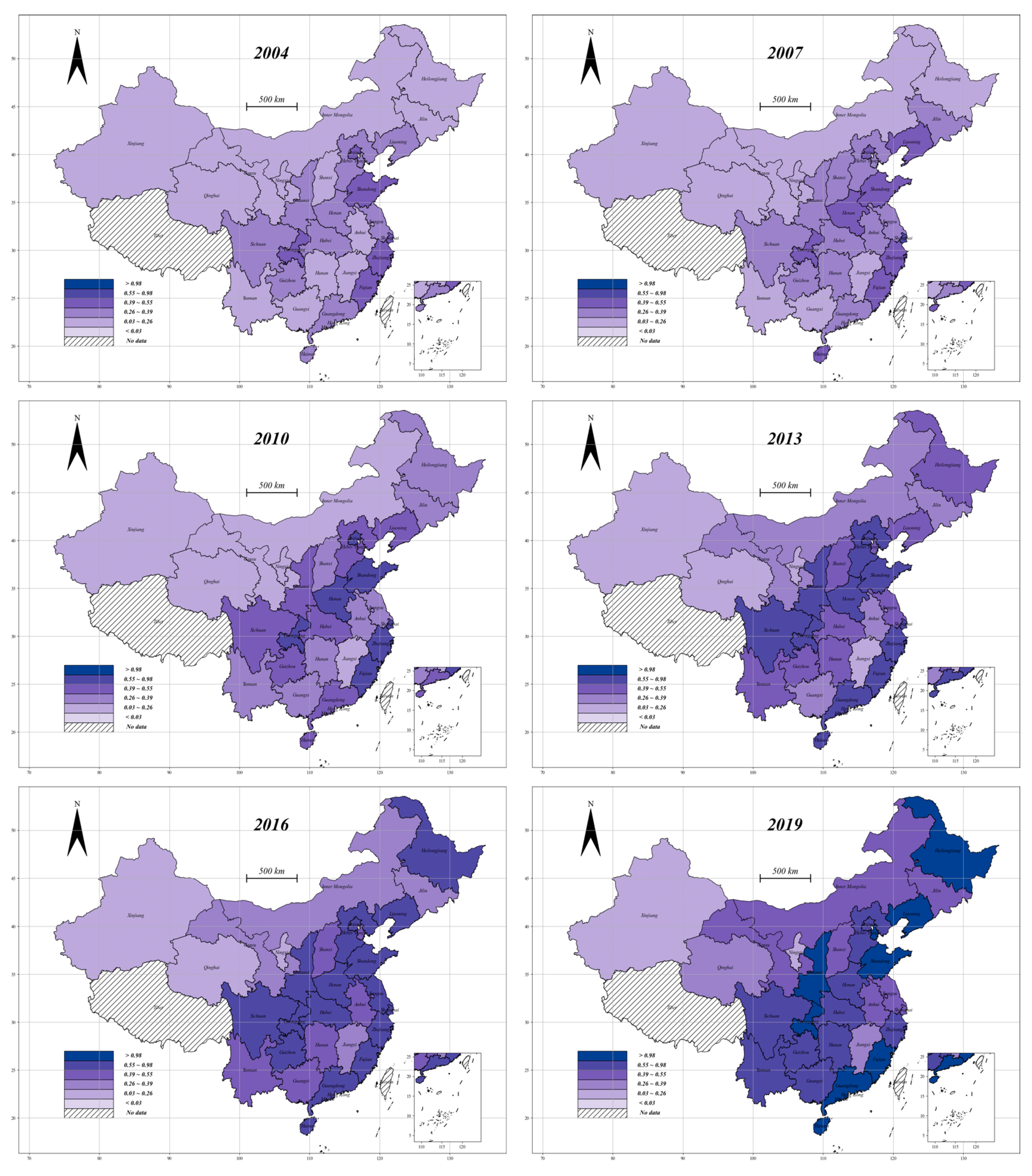
In addition, the variables that enter the DEA model are listed below. Fertilizer input is calculated using the quantity of nitrogen and phosphate fertilizer applied to agricultural produce. Pesticide input is measured in terms of the amount of pesticide used in agricultural output. The use of diesel in agricultural output acts as an index for energy input. Water input is proxied by total agricultural water usage. The total sown area acts as a proxy for land input. The agricultural planting industry is the focus of this research, and the yield value of the agriculture sector is employed as an indication of output value. In addition, to avoid the influence of inflation, the output value is deflated using 2002 as the base year.

Table 1. Summary statistics of agricultural production input and output.

Var Name	Unit	Mean	SD
Pesticide input	10 thousand ton	5.165	4.264
Fertilizer input	10 thousand ton	173.443	140.696
Energy input	10 thousand ton	63.562	65.914
Water input	100 million m3	119.801	101.188
Land input	1 thousand hectares	4201.223	3038.830
Output Value	100 million CNY	899.265	787.222

lists the variables that were used in the DEA model. Figure 3 depicts the regional distribution of IWE in China.

2.4. Econometric Model

This research investigates the impact of China’s IWE on ACE. As a consequence, ACE is the dependent variable, whereas IWE is the key independent variable. Because of the likely lag impact of ACE, this study empirically examines dynamic panel data; the econometric model is developed as follows:

$$LnAC{E}_{it}=\alpha +{\beta }_{0}LnAC{E}_{i,t-1}+{\beta }_{1}IW{E}_{it}+{\beta }_2{X}_{it}+{\epsilon }_{it}$$

(3)

where i denotes the cross-sectional individual and t denotes the number of time periods. _${\epsilon }_{it}$ is the random disturbance term that is independently and identically distributed, and α stands for the intercept term. ${\beta }_i$ (i ≥ 1) indicates the estimated coefficients. ACE denotes agricultural carbon emissions in the 30 Chinese provinces, IWE denotes irrigation water efficiency, and X represents a vector containing a number of controls, primarily level of urbanization (URB), industrial structure (IS), agricultural industrial structure (AIS), degree of water-saving irrigation (SAVE), and traffic development level (TDL).

Specifically, IWE is calculated according to Section 2.3, and ACE is measured according to Section 2.2. In addition, IS was measured by the ratio of the output value of tertiary industry to secondary industry. AIS is measured by the output of agro-processing industries over agricultural output. SAVE is measured as the ratio of irrigated area to total arable land. TDL is measured by dividing area road miles by arable land (km³/thousand hectare).

Table A2. Variable descriptive statistics.

VarName	Obs	Mean	SD	Min	Max
lnACE	540	0.992	0.954	−1.940	2.577
lnIWE	540	−1.031	0.690	−3.665	0.133
lnURB	540	−0.637	0.259	−1.314	0.258
lnIS	540	−0.035	0.370	−0.699	1.495
lnAIS	540	−1.270	0.907	−3.519	0.929
lnSAVE	540	−1.653	0.799	−3.333	0.304
lnTDL	540	0.993	0.869	−8.359	2.960
lnWSM	540	9.859	1.589	4.605	13.194
lnPSA	540	−2.155	0.770	−5.310	0.711

shows summary statistics (logarithmic) about these variables.

3. Results

The bulk of the empirical estimating methodologies used in this study are divided into three stages: (1) the Breusch–Pagan Lagrange multiplier (LM) and Pesaran cross-sectional dependence (CD) tests are used in this study to determine the presence of cross-sectional dependence within the panel data (Section 3.1); (2) a panel stationarity test using second-generation panel unit root test methods is used to determine the stationary of each variable (Section 3.2); and (3) the SYS-GMM is used as the reference approach for analyzing the effect of energy (Section 3.3).

3.1. Cross-Sectional Dependency Check

Before doing successful econometric analysis, it is required to evaluate the cross-sectional dependency within the panel data. Failure to do the cross-sectional dependency check may result in lack of consistency and poor dependability of the empirical data [28]. To execute the cross-sectional dependency check, this study used the Breusch–Pagan LM test [29], the Frees test [30], and the Pesaran CD test [31].

The results of the four cross-sectional dependence tests are shown in

Table 2. Cross-sectional dependency checks.

Test	Statistics	Prob.
Breusch–Pagan LM test	2891.89 ***	0.0000
Pesaran CD test	2.915 ***	0.0036
Frees test	2.817 ***	0.0000

Note: *** denotes significance at the 1% level.

. (i.e., the Breusch–Pagan LM test, the Frees test, and the Pesaran CD test). According to this table, all cross-sectional dependency checks’ p-value in this research are significant at a level of 1 percent, firmly rejecting the null hypothesis (i.e., no cross-sectional dependency occurs within the panel data). This means that the data units employed in this study’s cross-sectional sample are not independent. As a consequence, while conducting the following econometric empirical analysis, it is required to consider cross-sectional dependency inside the panel data.

3.2. Panel Stationarity Tsets

In order to avoid false regressions, it is required to check the panel data’s stationarity qualities after performing cross-sectional dependence tests on it. Importantly, when cross-sectional dependency occurs in panel data, the reliability of the first panel-unit-root-test (e.g., Levin-Lin-Chu (LLC), Im, Pesaran, and Shin (IPS), augmented Dickey–Fuller (ADF), and Phillips–Perron (PP) panel unit root tests) is considerably diminished [32]. As a result, Pesaran presents second-generation panel unit root test approaches that account for cross-sectional dependency, most notably the cross-sectional ADF (CADF) and cross-sectional IPS (CIPS) checks [32];

Table 3. Panel stationarity checks.

Variable	Level		1st Difference		Order of Integration
	Intercept	Intercept and Trend	Intercept	Intercept and Trend
Pesaran CADF test
LnACE	−1.797	−1.943	−3.821 ***	−3.940 ***	I (1)
LnIWE	−2.114 **	−2.270	−3.714 ***	−3.849 ***	I (1)
LnURB	−4.001 ***	−4.389 ***	−4.357 ***	−4.614 ***	I (1)
LnIS	−1.244	−2.541 *	−3.143 ***	−3.183 ***	I (1)
LnAIS	−2.040 *	−2.234	−3.684 ***	−3.960 ***	I (1)
LnSAVE	−1.784	−2.514	−3.947 ***	−3.942 ***	I (1)
LnTDL	−1.832	−2.139	−3.554 ***	−3.883 ***	I (1)
Pesaran CIPS test
LnACE	−1.938	−2.199	−3.775 ***	−3.940 ***	I (1)
LnIWE	−2.263 **	−2.602 *	−3.884 ***	−4.020 ***	I (1)
LnURB	−3.876 ***	−4.220 ***	−4.290 ***	−4.477 ***	I (1)
LnIS	−1.294	−2.614 *	−3.143 ***	−3.183 ***	I (1)
LnAIS	−2.030	−2.282 **	−3.766 ***	−3.860 ***	I (1)
LnSAVE	−1.784	−2.592 *	−3.947 ***	−3.942 ***	I (1)
LnTDL	−1.832	−2.139	−3.554 ***	−3.970 ***	I (1)

Notes: ***, **, and * denote statistical significance at the 1%, 5%, and 10% levels, respectively.

shows the findings for each variable.

Two types of root testing are highlighted by the panel unit root tests (i.e., intercept and intercept and trend). Table 3 shows that the initial sequence of the variables is not stationary, regardless of the trend term. The null hypothesis is rejected when the original data is subjected to first-order difference, and the p-values for the first-order sequence are significant at the 10% level (i.e., the panel data are not stationary). As a result, all variables are arranged in the same order (i.e., I (1)).

3.3. The Impact of IWE on ACE

This study is mainly concerned with identifying the influence of IWE on ACE, and since endogeneity difficulties may occur during the estimation procedure, correct econometric approaches must be used. The instrumental variable (IV) methodology is the most common and commonly utilized method for dealing with endogeneity. Furthermore, instrumental variables must be related to independent endogenous factors rather than the dependent variable’s disturbance term. Because these two goals often clash, it may be difficult to find important instrumental factors in practice. At the same time, lagging variables are often used as instrumental variables, thus the IV technique must generally match the spherical disturbance term assumption [33]. As a result, this study extensively uses the generalized method of moments (GMM), namely the difference GMM (DIF-GMM) developed by Arellano and Bond [34], as well as the SYS-GMM developed by Arellano and Bover [35] and Blundell and Bond [36]. In contrast to the DIF-GMM technique, the SYS-GMM method can effectively manage potential endogeneity and weak instrumentality issues by integrating the difference and level equations into a system equation for estimation [33]. As a result, this study estimates Equation (2) utilizing SYS-GMM as the benchmark approach, and the results are shown in the final column of

Table 4. Estimation of IWE–ACE nexus.

Variables	Static Panel Estimation			Dynamic Panel Estimation
	OLS	FE	RE	DIF-GMM	SYS-GMM
L.lnACE				0.579 ***	0.788 ***
				(0.0401)	(0.0391)
lnIWE	0.728 ***	0.608 ***	0.631 ***	0.366 ***	0.194 ***
	(0.0616)	(0.0691)	(0.0661)	(0.0483)	(0.0443)
lnURB	−0.148	−0.0628	−0.0859	−0.275 ***	−0.272 ***
	(0.188)	(0.129)	(0.127)	(0.0684)	(0.0876)
lnIS	−0.779 ***	−0.560 ***	−0.569 ***	−0.218 ***	−0.183 ***
	(0.105)	(0.0742)	(0.0734)	(0.0758)	(0.0467)
lnAIS	0.115 **	−0.0234	−0.0176	−0.0322 *	−0.0498 **
	(0.0544)	(0.0382)	(0.0376)	(0.0174)	(0.0204)
lnSAVE	−0.0185	0.0937	0.0533	−0.0858	−0.00274
	(0.0503)	(0.0829)	(0.0763)	(0.0873)	(0.0450)
lnTDL	−0.336 ***	−0.0202	−0.0292	0.00328	0.00266
	(0.0484)	(0.0323)	(0.0320)	(0.00696)	(0.00406)
Constant	2.070 ***	1.704 ***	1.663 ***	0.454 ***	0.173 *
	(0.162)	(0.139)	(0.193)	(0.160)	(0.0905)
AR (1)				0.0002	0.0004
AR (2)				0.5103	0.4088
Sargan test				0.999	0.999
Observations	540	540	540	480	510
R2	0.362	0.301	0.3

Notes: The symbols ***, **, and * reflect statistical significance at the 1%, 5%, and 10% levels, respectively; the values in parentheses represent standard error.

. Table 4 also contains the estimate results for the pooled ordinary least squares (OLS), fixed effect (FE), random effect (RE), and DIF-GMM techniques, which support the robustness of the empirical findings. The empirical results in this study are trustworthy and resilient since the sign and statistical significance of the variables are largely consistent throughout the five estimating strategies.

The Arellano–Bond (A–B) and Sargan tests are critical for analyzing dynamic panel data [37]. The former is primarily concerned with the autocorrelation properties of the difference term in the random disturbance term, while the latter is concerned with the efficacy of all instrumental variables employed in this research. In particular, the p-values for first-order (i.e., AR (1)) and second-order (i.e., AR (2)) differences in the last two columns of Table 4 are less than or equal to 0.1. This indicates that the SYS-GMM method is suitable for this inquiry. In addition, the Sargan test of the two-step GMM estimates produces non-significant p-values, suggesting that all instrumental variables utilized in this work are trustworthy. [38].

Following the establishment of IWE’s effects on ACE, this research examines the directional causality between IWE and ACE, providing more evidence for the IWE–ACE link. When cross-sectional dependence develops, the most often used causality test, the Granger causality test, is inapplicable [39]. Section 3.1, in particular, confirms the presence of cross-sectional dependency in the panel data; hence, this research applies Dumitrescu and Hurlin’s D-H panel causality test to evaluate the causative relationship of the IWE–ACE nexus [40]. The results showed that there was only a unidirectional causal relationship between IWE and ACE, IWE caused the increase in ACE (IWE→ACE: Z-bar = 1.8041, p-value = 0.0712; ACE→IWE: Z-bar = 1.2837, p-value = 0.1992).

For the control variables, URB has a negative effect on ACE, but only if the effect is statistically significant in the dynamic panel model. The Chinese government has been aggressively promoting urbanization in recent years, increasing carbon emissions from infrastructure construction, but the effect on agricultural carbon emissions remains unknown. The precise impact of urbanization on regional agricultural production, and thus on agricultural carbon emissions, is an intriguing subject worth investigating. The more advanced the region’s IS, the lower the ACE; the more advanced the IS, the lower the share of agriculture, and thus lower the emissions. The more advanced the agricultural industry structure, the lower the carbon emissions produced by agriculture. Advanced AIS implies high value added and low pollution, which contributes to the reduction of agricultural carbon emissions. Advanced AIS, on the other hand, will undoubtedly increase the efficiency of input factors and eliminate unnecessary waste. The coefficient of SAVE’s effect on ACE fails the significance test. Only in OLS is the coefficient of the effect of TDL on ACE significant. This indicates that the effects of SAVE and TDL on ACE are not robust, that their mechanisms of action may be complex, and that their mechanisms of action should be further elucidated.

4. Further Discussion

4.1. An Asymmetric Examination of the Influence of IWE on ACE

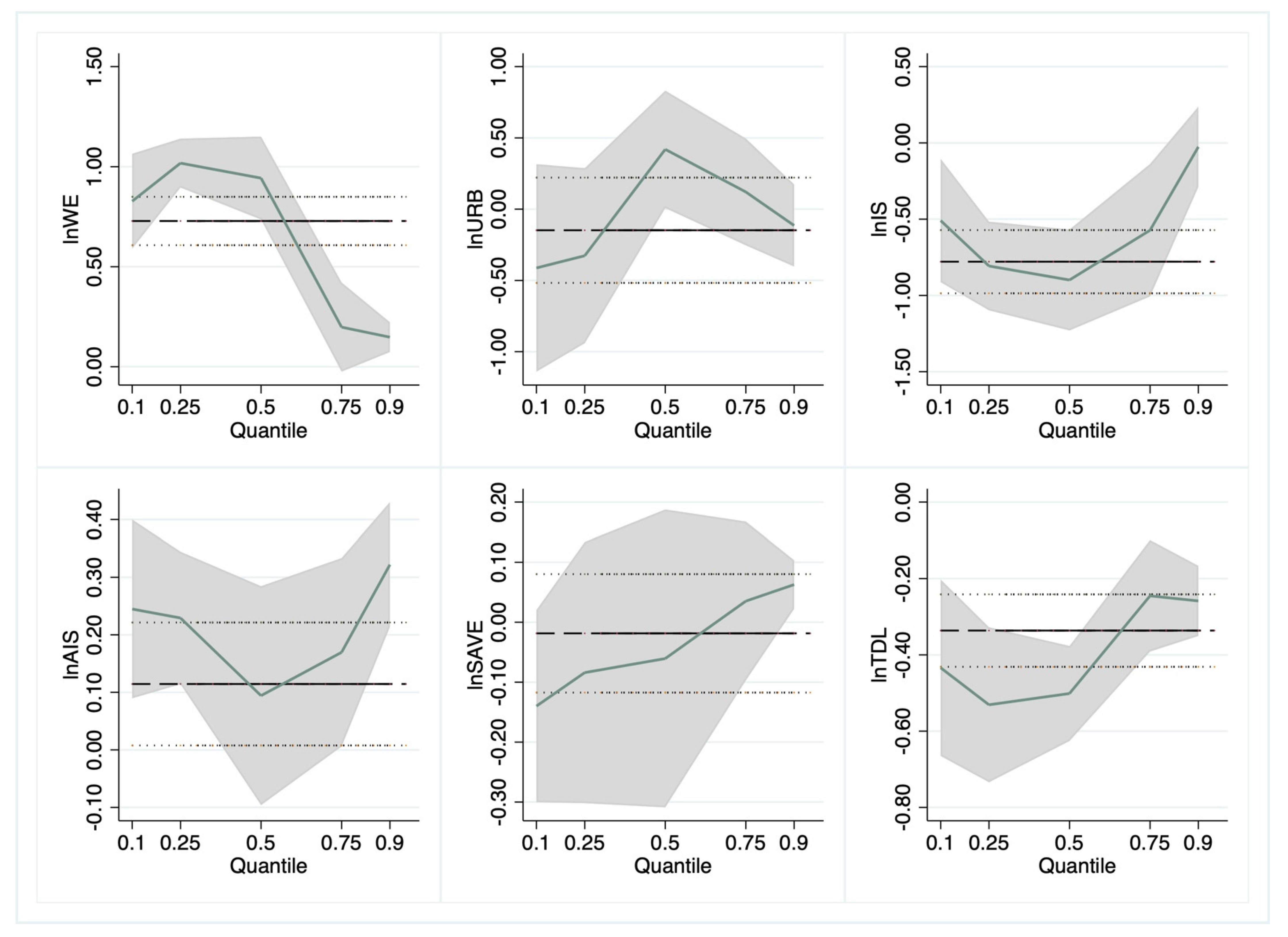
This paper estimates Equation (2) based on the two-step panel quantile regression for the 10th, 25th, 50th, 75th, and 90th percentiles of the conditional ACE to perform a quantitative evaluation of the asymmetric structure of the influence of IWE on ACE. Canay proposed a two-step panel quantile technique to overcome unobserved individual heterogeneity [41]. The estimation results are summarized in

Table 5. Estimation of two-step panel quantile regression.

Dependent Variable: lnACE
Variables	Quantiles
	q10	q25	q50	q75	q90
lnIWE	0.537 ***	0.526 ***	0.580 ***	0.631 ***	0.708 ***
	(0.0570)	(0.0257)	(0.0196)	(0.0321)	(0.0406)
lnURB	−0.0261	−0.284 ***	−0.146	0.101	−0.0310
	(0.196)	(0.0688)	(0.0897)	(0.138)	(0.135)
lnIS	−0.665 ***	−0.442 ***	−0.443 ***	−0.479 ***	−0.630 ***
	(0.141)	(0.0628)	(0.0583)	(0.0668)	(0.136)
lnAIS	0.00442	0.0555 *	0.0150	−0.0646 *	−0.0878 **
	(0.0489)	(0.0325)	(0.0270)	(0.0390)	(0.0417)
lnSAVE	0.0823 *	0.0733 ***	0.0887 ***	0.0692 ***	0.139 ***
	(0.0438)	(0.0278)	(0.0174)	(0.0268)	(0.0470)
lnTDL	−0.00134	0.0153	−0.00428	−0.0316	−0.0795
	(0.0405)	(0.0196)	(0.0142)	(0.0235)	(0.0497)
Constant	1.281 ***	1.367 ***	1.649 ***	1.917 ***	2.255 ***
	(0.131)	(0.0549)	(0.0496)	(0.102)	(0.184)
R-squared	0.4424	0.4454	0.4310	0.3918	0.3669

Notes: ***, **, and * denote statistical significance at the 1%, 5%, and 10% levels, respectively; values in parentheses represent standard errors.

. Furthermore, Figure 4 depicts the distinct patterns of change in the coefficients of influencing factors at different quantile levels.

IWE had a positive effect on ACE that passed the significance test, and the effect of IWE became increasingly significant as ACE increased. This demonstrates that in high-carbon agricultural regions, increasing irrigation efficiency is a significant driver of GHG emissions. In the region with higher agricultural carbon emissions, energy consumption invested in improving irrigation efficiency has a diminishing marginal effect, implying that more energy is required to improve irrigation efficiency, resulting in increased ACE. The agricultural industry’s structure demonstrates the effect of ACE reduction only during the high ACE stage. This partially confirms the environmental Kuznets curve, namely that as emissions increase, the economic level continues to develop until it reaches an inflection point, at which point economic development can contribute to emission reduction.

4.2. Heterogeneous Analysis of the Impact of IWE on ACE

This research divides 30 provinces in China into southern and northern regions based on geographic location to further investigate the regional heterogeneity influence of IWE on ACE; the relevant subpanels are presented in

Table A1. The specific provinces across different regions.

Region	Provinces
North (15 provinces)	Beijing, Hebei, Tianjin, Inner Mongolia, Shanxi, Jilin, Liaoning, Heilongjiang, Henan, Shandong, Gansu, Shaanxi, Ningxia, Qinghai, Xinjiang
South (15 provinces)	Shanghai, Jiangsu, Hainan, Fujian, Hubei, Jiangxi, Guangxi, Hunan, Guangdong, Sichuan, Guizhou, Chongqing, Zhejiang, Anhui, Yunnan

.

Table 6. Results of the region’s heterogeneous analysis.

Variables	North	South
lnIWE	0.953 ***	0.726 ***
	(0.0816)	(0.0797)
lnURB	−0.177	−0.00917
	(0.187)	(0.170)
lnIS	−0.660 ***	−1.037 ***
	(0.106)	(0.124)
lnAIS	0.118 **	0.0904
	(0.0543)	(0.0565)
lnSAVE	0.138 **	−0.308 ***
	(0.0624)	(0.0437)
lnTDL	−0.568 ***	−0.114 *
	(0.0650)	(0.0665)
Constant	2.644 ***	1.444 ***
	(0.204)	(0.200)
Modified Wald Statistic	21,649.70 ***	3881.87 ***

Notes: ***, **, and * indicate statistical significance at the 1%, 5%, and 10% levels, respectively; the values in parentheses represent standard errors.

shows the estimate results based on the FGLS approach.

One of the main reasons why IWE leads to more ACE in the north is that irrigation in the north relies more on groundwater irrigation, which requires more energy to pump. The abatement effect of IS advances is more pronounced in the south, possibly because the South is more economically developed and better able to leverage the abatement effect of enhanced IS. Interestingly, the impact of SAVE on ACE is quite different due to regional differences. China requires irrigation for 70% of grain, 80% of cotton, and 90% of vegetable production. Northern China has 19% of the water resources, 65% of arable land, and produces 50% of food [6]. Moreover, northern China is facing severe groundwater overdraft, the groundwater level is decreasing, and the extraction of groundwater consumes a lot of energy, which leads to a large amount of greenhouse gas emissions [11]. Therefore, expanding irrigated areas in the north is undoubtedly exacerbating greenhouse gas emissions. Increasing irrigated areas in the south is not as costly in terms of energy consumption as in the north, and the increased water input helps to reduce the substitution of other energy-consuming factors of production to some extent, thus reducing ACE instead.

4.3. Mediation Impact Mechanism

Increased irrigation efficiency may lower the cost of agricultural production, but it may also increase the scale of irrigation [13,18], resulting in more intensive irrigation activities, and thus not achieving a reduction in ACE by reducing total water use. As an outcome, increased irrigation efficiency may result in increased ACE levels as a result of increased irrigation scale. Second, increased irrigation efficiency facilitates farmer irrigation activities and increases farmer irrigation capacity, which may induce farmers to shift to cash crops and reduce food crop cultivation, for example, by increasing vegetable cultivation, which can be more profitable than food crop cultivation. Food crop cultivation generates a significant amount of greenhouse gases [9,15], and reducing food crop cultivation can help reduce ACE. Simultaneously, vegetable cultivation requires meticulous management, which promotes energy efficiency in agricultural production and thus reduces greenhouse gas emissions. On the other hand, food crop cultivation is more primitive in terms of production methods and input factors, which is not as refined as vegetable cultivation.

The number of agricultural water-saving irrigation facilities machinery (WSM) as an indicator of the scale of irrigation, the proportion of vegetable planting area as an indicator of planting structure adjustment (PSA). Descriptive statistics of the variables are shown in Table A2. The mediating effect model used to analyze the mechanism is established as follows:

$$LnAC{E}_{it}={\delta }_{1}LnIW{E}_{it}+{\beta }_1{X}_{it}+{\varphi }_{it}$$

(4)

$$Ln{M}_{it}={\delta }_{2}LnIW{E}_{it}+{\beta }_2{X}_{it}+{\mu }_{it}$$

(5)

$$LnAC{E}_{it}={\delta }_{3}LnIW{E}_{it}+{\delta }_{4}Ln{M}_{it}+{\beta }_3{X}_{it}+{\gamma }_{it}$$

(6)

where i denotes the cross-sectional unit of analysis (province) and t denotes the number of time periods (year). where $ACE$ represent province-level agricultural carbon emissions. $IWE$ denotes irrigation water efficiency, $X$ indicates a series of control factors. $M$ represent mediators, including WSM and PSA. ${\delta }_1$ is the total effects of IWE on ACE. ${\delta }_3$ denote the direct effect of IWE on ACE. Furthermore, ${\delta }_2·{\delta }_4$ are the indirect effect.

Table 7. Results of the mechanism analysis.

Variables	(1)	(2)	(3)	(4)
	lnWSM	lnPSA	lnACE	lnACE
lnWSM			0.195 ***
			(0.0165)
lnPSA				−0.339 ***
				(0.0386)
lnIWE	0.470 ***	0.520 ***	0.727 ***	0.971 ***
	(0.0760)	(0.0350)	(0.0531)	(0.0518)
lnURB	−0.603 **	−0.483 ***	0.329 ***	−0.0161
	(0.234)	(0.107)	(0.111)	(0.116)
lnIS	−0.797 ***	0.115 **	−0.792 ***	−0.845 ***
	(0.0907)	(0.0479)	(0.0692)	(0.0665)
lnAIS	0.796 ***	−0.132 ***	−0.111 ***	0.0273
	(0.0588)	(0.0287)	(0.0359)	(0.0344)
lnSAVE	0.0662	0.0546 **	−0.117 ***	−0.0505
	(0.0598)	(0.0250)	(0.0330)	(0.0390)
lnTDL	−0.233 ***	0.420 ***	−0.250 ***	−0.196 ***
	(0.0578)	(0.0365)	(0.0405)	(0.0475)
Constant	11.37 ***	−2.362 ***	−0.117	1.334 ***
	(0.180)	(0.107)	(0.216)	(0.178)
Modified Wald Statistic	43,036.12 ***	5120.82 ***	14,671.02 ***	6111.77 ***
Observations	540	540	540	540
Province	30	30	30	30

Notes: ***, and **, indicate statistical significance at the 1%, 5%, and 10% levels, respectively; the values in parentheses represent standard errors.

reports the estimated results of the mediating effect analysis, which indicate that the effect of IWE on ACE is mediated partially by PSA and WSM, and their coefficients pass the significance test. IWE increases ACE by increasing WSM, which partially responds to the irrigation paradox; consequently, increasing IWE cannot be a highly effective tool for reducing ACE. IWE contributes to the reduction of ACE by promoting PSA, which has significant policy implications. PSA is critical in reducing ACE as a result of the IWE drive. As a consequence, the government should mitigate IWE’s positive effect on ACE by encouraging crop restructuring and limiting the expansion of ineffective and crude irrigation scales.

5. Conclusions and Policy Implications

This research used empirical analysis on a balanced panel dataset encompassing China’s 30 provinces from 2002 to 2019 to evaluate the dynamic links between IWE and ACE in a systematic manner. Given the panel’s possible cross-sectional dependency and stationarity, the IWE–ACE nexus is determined using SYS-GMM as the benchmark approach. Additionally, the asymmetry of IWE’s effect on ACE is examined for the whole panel, as well as the heterogeneity among regions and possible mechanisms. The followings are the study’s key findings:

• China’s agricultural carbon emissions have generally increased, though at a slower rate in recent years. China’s agricultural carbon emissions vary significantly by region, with relatively high levels in northern regions and eastern coastal provinces. Irrigation efficiency in China also varies by region, being particularly low in the north;
• Due to the growing economic integration of provinces, there is a high degree of interdependence between them. Additionally, the study’s major finding indicates that IWE has a positive effect on ACE. More precisely, a rise of 1% in IWE results in an increase of 0.194% in ACE;
• The results of asymmetric analysis demonstrate that as ACE increases, the impact of IWE becomes more significant. The analysis of regional differences reveals that IWE has a greater influence on ACE in the north;
• Mechanism analysis demonstrates that IWE can reduce ACE by promoting planting structure adjustment. IWE can increase ACE by boosting irrigation scales. PSA and WSM play a partially mediating role in the IWE–ACE relationship.

The empirical findings discussed above have policy implications. To begin, empirical evidence suggests that IWE has a generally positive effect on ACE. Thus, considering the positive effect of IWE on ACE and taking appropriate measures is critical for ensuring irrigation efficiency and emission reduction. To be more precise, the government should avoid excessive energy input in order to maximize irrigation efficiency, develop low-energy irrigation equipment, and implement more advanced water-saving equipment and management practices.

Second, the impact of IWE increases as ACE levels rise. In the north, ACE is more susceptible to IWE. With less water and more arable land, the north produces half of the country’s food. The resulting problems must be considered; for example, excessive groundwater extraction can result in a drop in the water table, forcing the use of more energy to pump water. The north is experiencing more droughts as a result of climate change, and the response to droughts is to increase the frequency and amount of irrigation, necessitating higher irrigation efficiency to conserve water. Combating drought requires increased irrigation, which undoubtedly results in an increase in agricultural carbon emissions. Therefore, northern China should establish irrigation quotas and restrict total water use to avoid increased irrigation efficiency resulting in increased water resource exploitation, thereby avoiding increased agricultural carbon emissions. Other more water-efficient strategies for combating climate change should be considered as well. For example, enhance irrigation management and set irrigation limits to avoid excessive waste of water. Promote drought-resistant and water-saving crop varieties.

Finally, an examination of possible impact mechanisms reveals two critical mediating variables: irrigation scale and crop structure. Increased irrigation efficiency expands irrigation scale, resulting in more intensive irrigation activities, which results in increased agricultural carbon emissions. Increased water efficiency, on the other hand, promotes crop restructuring by reducing the cultivation of food crops that generate significant amounts of greenhouse gases and increasing the cultivation of cash crops. Cash crops might improve energy efficiency and reduce agricultural carbon emissions as a result of more prudent management. As a consequence, the government should restrict the expansion of inefficient and crude irrigation systems and encourage the cultivation of water-efficient and low-carbon-emitting crops.

References

- Zhao, J.; Jiang, Q.; Dong, X.; Dong, K.; Jiang, H. How Does Industrial Structure Adjustment Reduce CO2 Emissions? Spatial and Mediation Effects Analysis for China. Energy Econ. 2022, 105, 105704. [Google Scholar] [CrossRef]
- Zhao, J.; Jiang, Q.; Dong, X.; Dong, K. Assessing Energy Poverty and Its Effect on CO2 Emissions: The Case of China. Energy Econ. 2021, 97, 105191. [Google Scholar] [CrossRef]
- Yang, H.; Wang, X.; Bin, P. Agriculture Carbon-Emission Reduction and Changing Factors behind Agricultural Eco-Efficiency Growth in China. J. Clean. Prod. 2022, 334, 130193. [Google Scholar] [CrossRef]
- Huang, Q.; Wang, J.; Li, Y. Do Water Saving Technologies Save Water? Empirical Evidence from North China. J. Environ. Econ. Manag. 2017, 82, 1–16. [Google Scholar] [CrossRef]
- Zhang, T.; Wang, J.; Teng, Y. Adaptive Effectiveness of Irrigated Area Expansion in Mitigating the Impacts of Climate Change on Crop Yields in Northern China. Sustainability 2017, 9, 851. [Google Scholar] [CrossRef] [Green Version]
- Wang, J.; Zhu, Y.; Sun, T.; Huang, J.; Zhang, L.; Guan, B.; Huang, Q. Forty Years of Irrigation Development and Reform in China. Aust. J. Agric. Resour. Econ. 2020, 64, 126–149. [Google Scholar] [CrossRef]
- Shi, H. Performance of Community-Based Water-Saving Technology under Land Fragmentation: Evidence from Groundwater Overexploitation in the North China Plain. Water Policy 2021, 23, 1542–1555. [Google Scholar] [CrossRef]
- Pardo, M.Á.; Riquelme, A.J.; Jodar-Abellan, A.; Melgarejo, J. Water and Energy Demand Management in Pressurized Irrigation Networks. Water 2020, 12, 1878. [Google Scholar] [CrossRef]
- Feng, Z.Y.; Qin, T.; Du, X.Z.; Sheng, F.; Li, C.F. Effects of Irrigation Regime and Rice Variety on Greenhouse Gas Emissions and Grain Yields from Paddy Fields in Central China. Agric. Water Manag. 2021, 250, 106830. [Google Scholar] [CrossRef]
- Siyal, A.W.; Gerbens-Leenes, P.W.; Nonhebel, S. Energy and Carbon Footprints for Irrigation Water in the Lower Indus Basin in Pakistan, Comparing Water Supply by Gravity Fed Canal Networks and Groundwater Pumping. J. Clean. Prod. 2021, 286, 125489. [Google Scholar] [CrossRef]
- Qiu, G.Y.; Zhang, X.; Yu, X.; Zou, Z. The Increasing Effects in Energy and GHG Emission Caused by Groundwater Level Declines in North China’s Main Food Production Plain. Agric. Water Manag. 2018, 203, 138–150. [Google Scholar] [CrossRef]
- Zou, X.; Li, Y.; Li, K.; Cremades, R.; Gao, Q.; Wan, Y.; Qin, X. Greenhouse Gas Emissions from Agricultural Irrigation in China. Mitig. Adapt. Strateg. Glob. Change 2015, 20, 295–315. [Google Scholar] [CrossRef] [Green Version]
- Borsato, E.; Martello, M.; Marinello, F.; Bortolini, L. Environmental and Economic Sustainability Assessment for Two Different Sprinkler and A Drip Irrigation Systems: A Case Study on Maize Cropping. Agriculture 2019, 9, 187. [Google Scholar] [CrossRef] [Green Version]
- Melián-Navarro, A.; Ruiz-Canales, A. Evaluation in Carbon Dioxide Equivalent and CHG Emissions for Water and Energy Management in Water Users Associations. A Case Study in the Southeast of Spain. Water 2020, 12, 3536. [Google Scholar] [CrossRef]
- Nasseri, A. Energy Use and Economic Analysis for Wheat Production by Conservation Tillage along with Sprinkler Irrigation. Sci. Total Environ. 2019, 648, 450–459. [Google Scholar] [CrossRef]
- Belaud, G.; Mateos, L.; Aliod, R.; Buisson, M.-C.; Faci, E.; Gendre, S.; Ghinassi, G.; Gonzales Perea, R.; Lejars, C.; Maruejols, F.; et al. IRRIGATION AND ENERGY: ISSUES AND CHALLENGES. Irrig. Drain. 2020, 69, 177–185. [Google Scholar] [CrossRef]
- Handa, D.; Frazier, R.; Taghvaeian, S.; Warren, J. The Efficiencies, Environmental Impacts and Economics of Energy Consumption for Groundwater-Based Irrigation in Oklahoma. Agriculture 2019, 9, 27. [Google Scholar] [CrossRef] [Green Version]
- McCarthy, B.; Anex, R.; Wang, Y.; Kendall, A.D.; Anctil, A.; Haacker, E.M.K.; Hyndman, D.W. Trends in Water Use, Energy Consumption, and Carbon Emissions from Irrigation: Role of Shifting Technologies and Energy Sources. Environ. Sci. Technol. 2020, 54, 15329–15337. [Google Scholar] [CrossRef]
- Wang, H.; Zhang, Y.; Zhang, Y.; McDaniel, M.D.; Sun, L.; Su, W.; Fan, X.; Liu, S.; Xiao, X. Water-Saving Irrigation Is a ‘Win-Win’ Management Strategy in Rice Paddies—With Both Reduced Greenhouse Gas Emissions and Enhanced Water Use Efficiency. Agric. Water Manag. 2020, 228, 105889. [Google Scholar] [CrossRef]
- Minli, Y.; Minzan, L.; Xiwen, L. 50 Years of Agricultural Mechanization in China. AMA Agric. Mech. Asia Afr. Lat. Am. 2020, 51, 86–92. [Google Scholar]
- Guan, Y.; Shan, Y.; Huang, Q.; Chen, H.; Wang, D.; Hubacek, K. Assessment to China’s Recent Emission Pattern Shifts. Earth’s Future 2021, 9, e2021EF002241. [Google Scholar] [CrossRef]
- Shan, Y.; Huang, Q.; Guan, D.; Hubacek, K. China CO2 Emission Accounts 2016–2017. Sci. Data 2020, 7, 54. [Google Scholar] [CrossRef] [PubMed] [Green Version]
- Shan, Y.; Guan, D.; Zheng, H.; Ou, J.; Li, Y.; Meng, J.; Mi, Z.; Liu, Z.; Zhang, Q. China CO2 Emission Accounts 1997–2015. Sci. Data 2018, 5, 170201. [Google Scholar] [CrossRef] [PubMed] [Green Version]
- Shan, Y.; Liu, J.; Liu, Z.; Xu, X.; Shao, S.; Wang, P.; Guan, D. New Provincial CO2 Emission Inventories in China Based on Apparent Energy Consumption Data and Updated Emission Factors. Appl. Energy 2016, 184, 742–750. [Google Scholar] [CrossRef] [Green Version]
- IPCC. IPCC Climate Change 2007: Mitigation: Contribution of Working Group III to the Fourth Assessment Report of the Intergovernmental Panel on Climate Change: Summary for Policymakers and Technical Summary; Cambridge University Press: Cambridge, UK, 2007. [Google Scholar]
- Tang, J.; Folmer, H.; Xue, J. Technical and Allocative Efficiency of Irrigation Water Use in the Guanzhong Plain, China. Food Policy 2015, 50, 43–52. [Google Scholar] [CrossRef]
- Chang, M.; Liu, J.; Shi, H.; Guo, T. The Effect of Off-Farm Employment on Agricultural Production Efficiency: Micro Evidence in China. Sustainability 2022, 14, 3385. [Google Scholar] [CrossRef]
- Grossman, G.M.; Krueger, A.B. Economic Growth and the Environment. Q. J. Econ. 1995, 110, 353–377. [Google Scholar] [CrossRef] [Green Version]
- Breusch, T.S.; Pagan, A.R. The Lagrange Multiplier Test and Its Applications to Model Specification in Econometrics. Rev. Econ. Stud. 1980, 47, 239. [Google Scholar] [CrossRef]
- Frees, E.W. Longitudinal and Panel Data: Analysis and Applications in the Social Sciences; Cambridge University Press: Cambridge, UK, 2004. [Google Scholar]
- Pesaran, M.H. General Diagnostic Tests for Cross Section Dependence in Panels; Cambridge University Press: Cambridge, UK, 2004. [Google Scholar] [CrossRef]
- Pesaran, M.H. A Simple Panel Unit Root Test in the Presence of Cross-Section Dependence. J. Appl. Econ. 2007, 22, 265–312. [Google Scholar] [CrossRef] [Green Version]
- Bun, M.J.G.; Windmeijer, F. The Weak Instrument Problem of the System GMM Estimator in Dynamic Panel Data Models. Econom. J. 2010, 13, 95–126. [Google Scholar] [CrossRef] [Green Version]
- Arellano, M.; Bond, S. Some Tests of Specification for Panel Data: Monte Carlo Evidence and an Application to Employment Equations. Rev. Econ. Stud. 1991, 58, 277. [Google Scholar] [CrossRef] [Green Version]
- Arellano, M.; Bover, O. Another Look at the Instrumental Variable Estimation of Error-Components Models. J. Econom. 1995, 68, 29–51. [Google Scholar] [CrossRef] [Green Version]
- Blundell, R.; Bond, S. Initial Conditions and Moment Restrictions in Dynamic Panel Data Models. J. Econom. 1998, 87, 115–143. [Google Scholar] [CrossRef] [Green Version]
- Che, Y.; Lu, Y.; Tao, Z.; Wang, P. The Impact of Income on Democracy Revisited. J. Comp. Econ. 2013, 41, 159–169. [Google Scholar] [CrossRef] [Green Version]
- Roodman, D. How to Do Xtabond2: An Introduction to Difference and System GMM in Stata. Stata J. 2009, 9, 86–136. [Google Scholar] [CrossRef] [Green Version]
- Granger, C.W.J. Investigating Causal Relations by Econometric Models and Cross-Spectral Methods. Econometrica 1969, 37, 424. [Google Scholar] [CrossRef]
- Dumitrescu, E.-I.; Hurlin, C. Testing for Granger Non-Causality in Heterogeneous Panels. Econ. Model. 2012, 29, 1450–1460. [Google Scholar] [CrossRef] [Green Version]
- Canay, I.A. A Simple Approach to Quantile Regression for Panel Data. Econom. J. 2011, 14, 368–386. [Google Scholar] [CrossRef]
Figure 1.
China’s agricultural carbon emissions over time (unit: Mt).
Figure 2.
Spatial distribution of agricultural carbon emissions in China (unit: Mt).
Figure 3.
Spatial distribution of irrigation water efficiency in China.
Figure 4.
Change in panel quantile regression coefficients. Notes: the x-axis represents the conditional quantiles of ACE and y-axis denotes the coefficient values of various variables. The black line indicates the coefficient values of panel data model with fixed effect.