
Modern Techniques to Modeling Reference Evapotranspiration in a Semiarid Area Based on ANN and GEP Models

 ,
,  ,
,  ,
,  ,
,  ,
, 
Abstract
:1. Introduction
2. Materials and Methods
2.1. Study Area and Meteorological Data Acquisition
2.2. Description of Data
2.3. Evapotranspiration Estimation Method
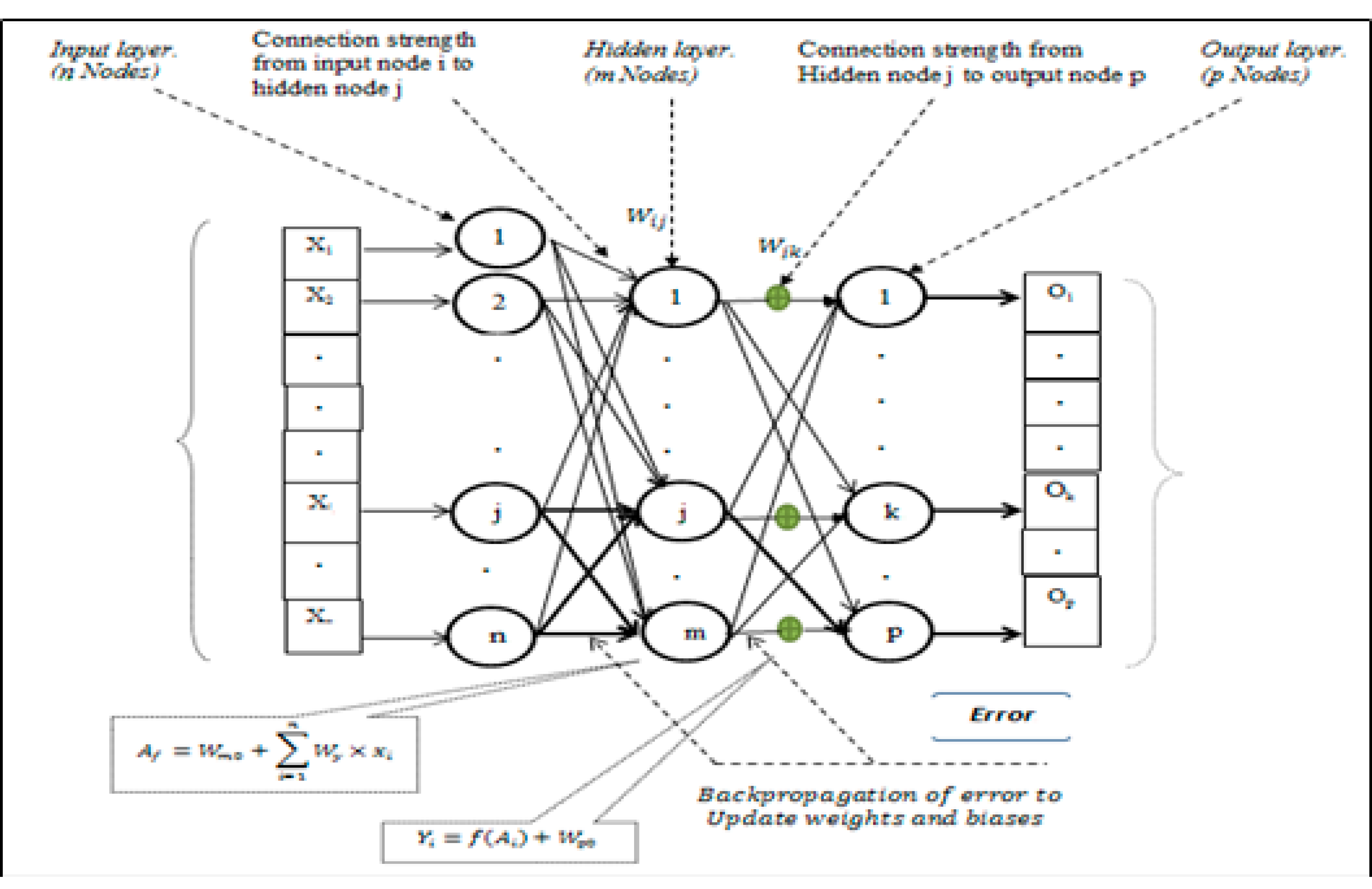
2.4. Multilayer Perceptron Artificial Neural Network
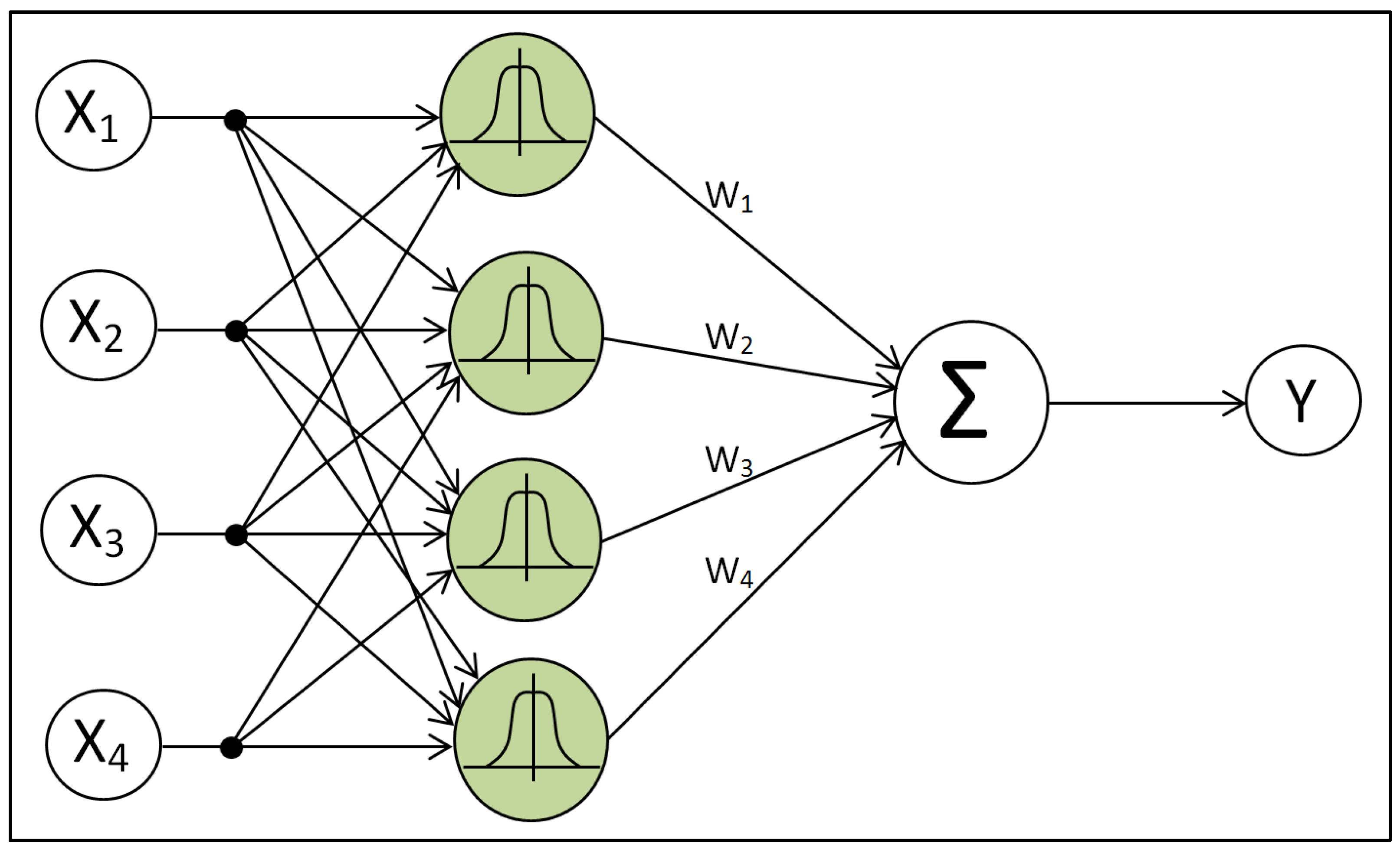
2.5. Radial Basis Function
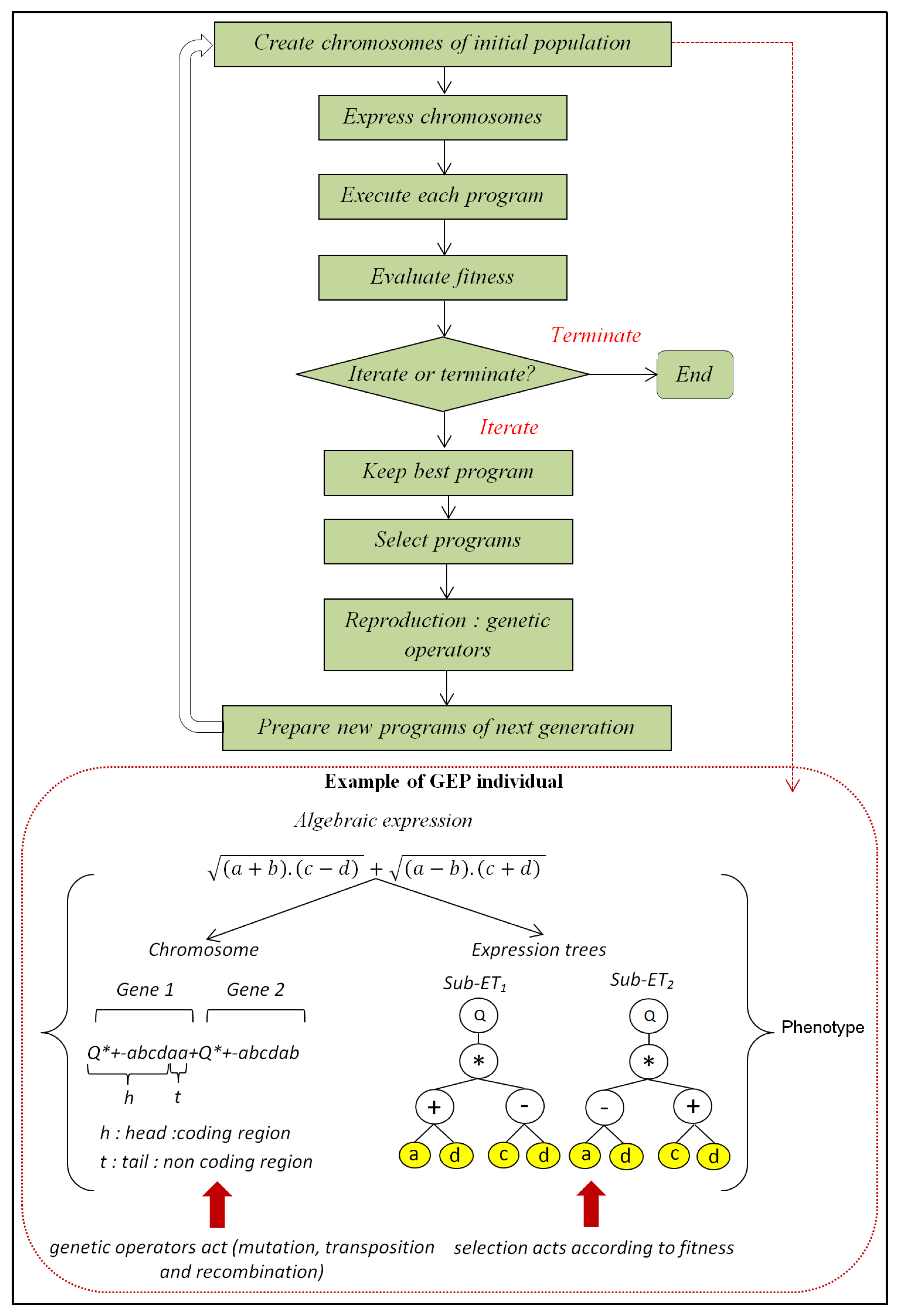
2.6. Gene Expression Programming
2.7. Evaluation Criteria
3. Results and Discussion
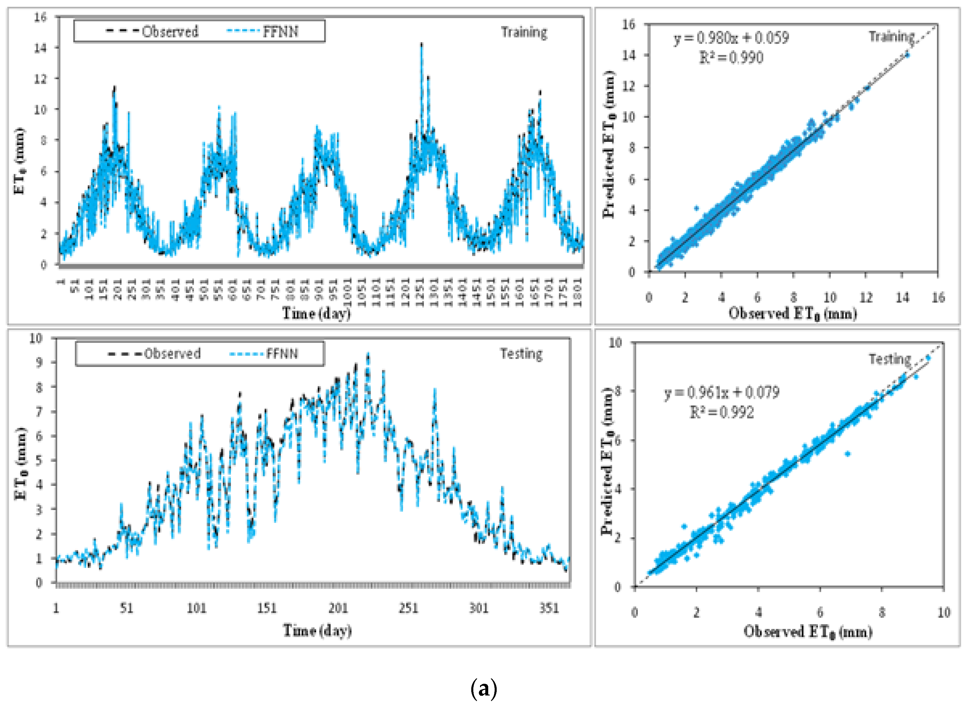
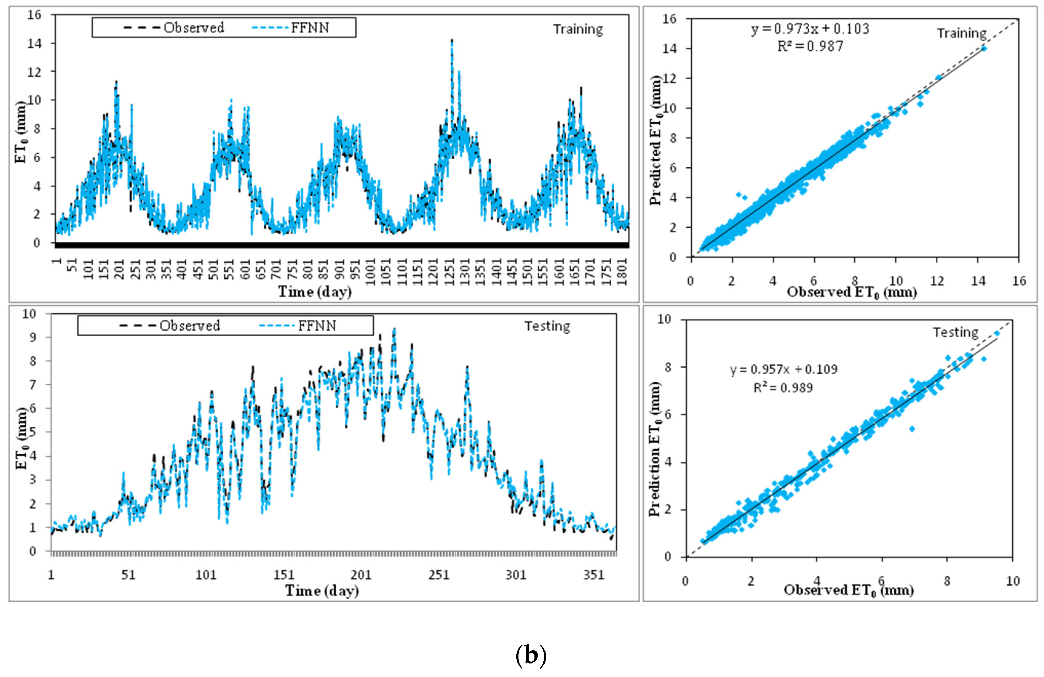
3.1. Application of MLP
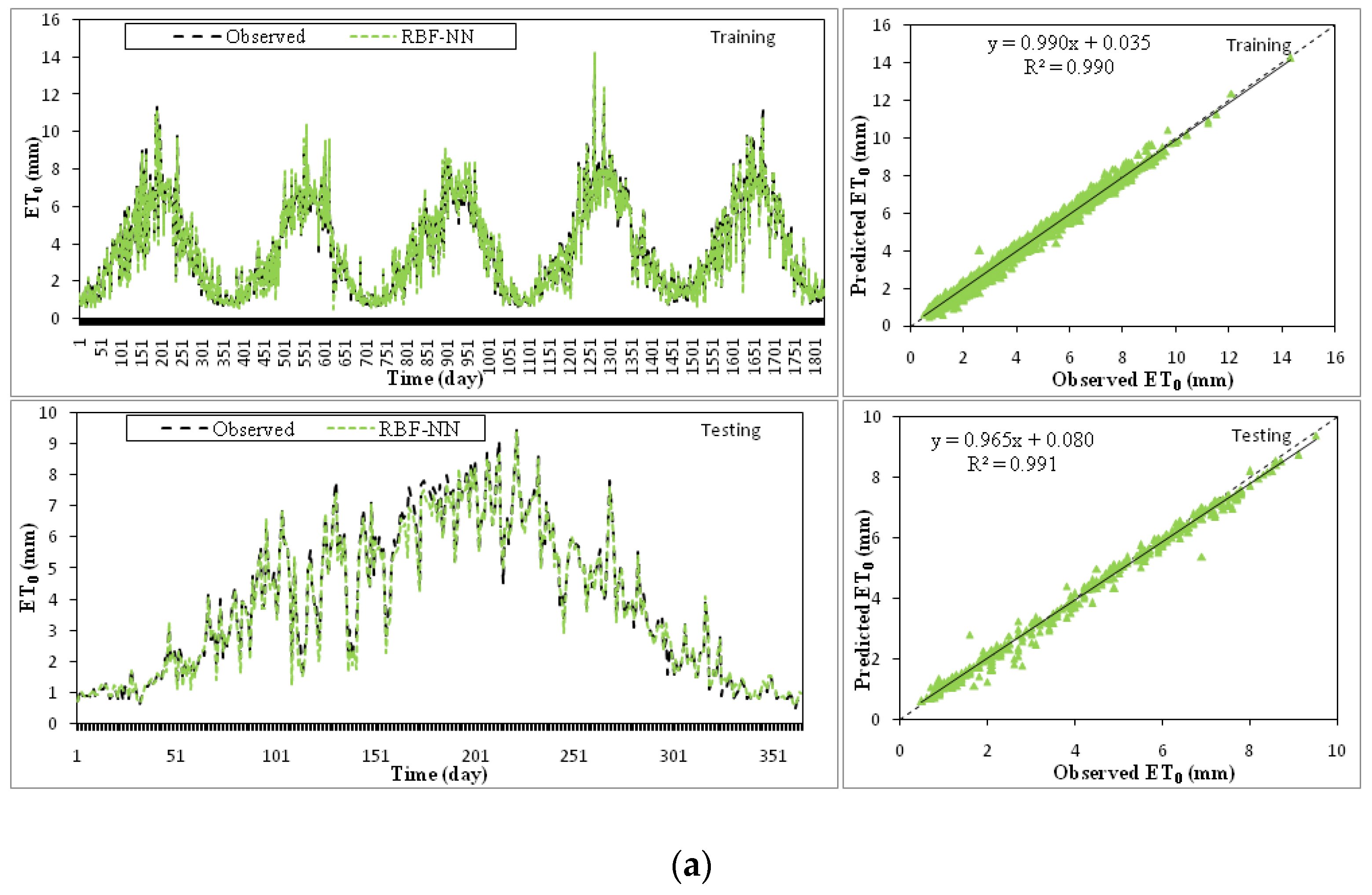
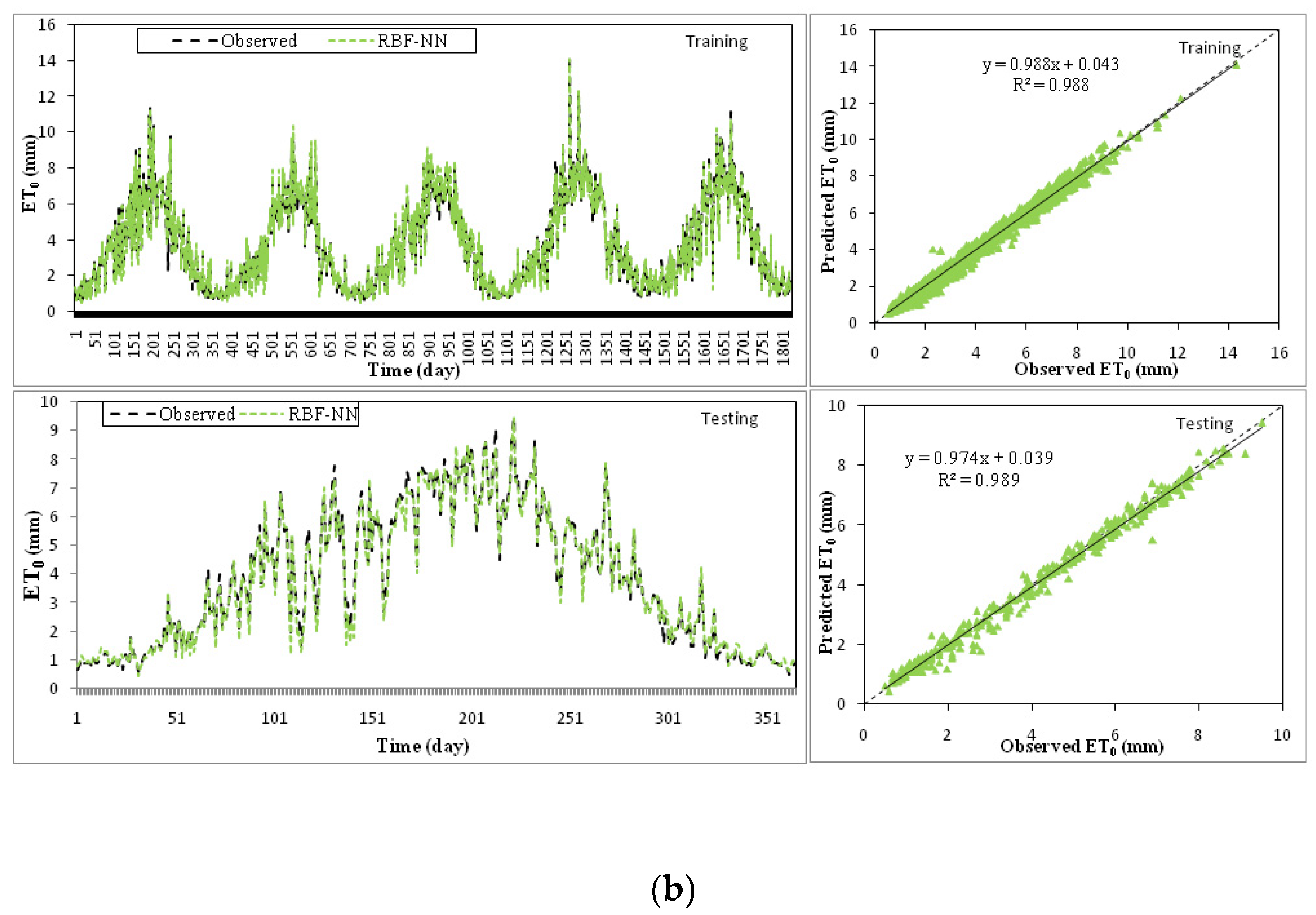
3.2. Application of RBF
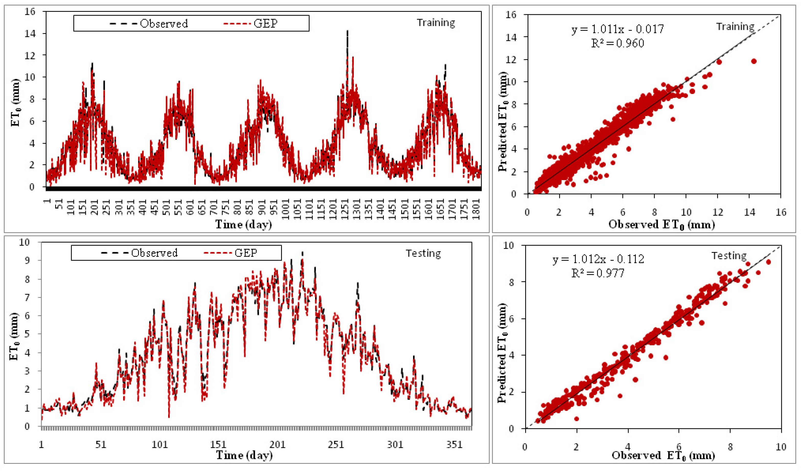
3.3. Application of GEP
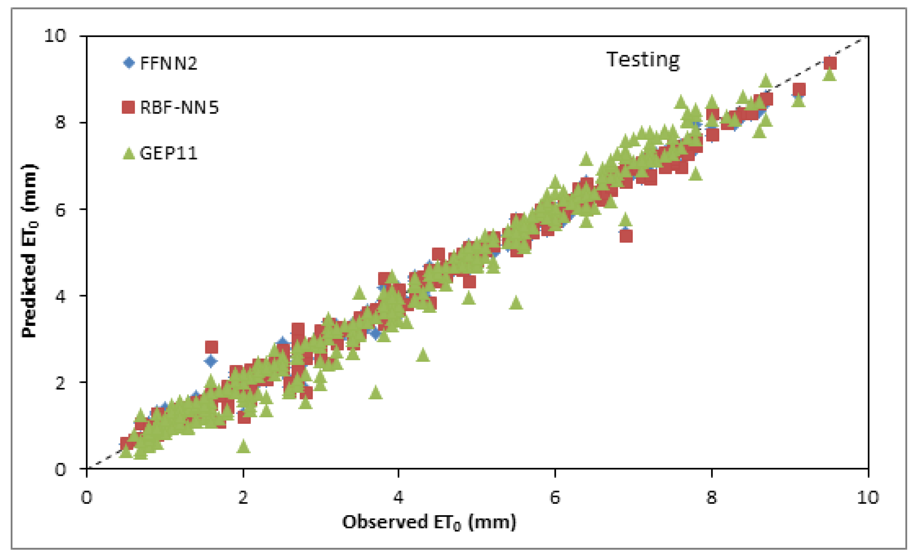
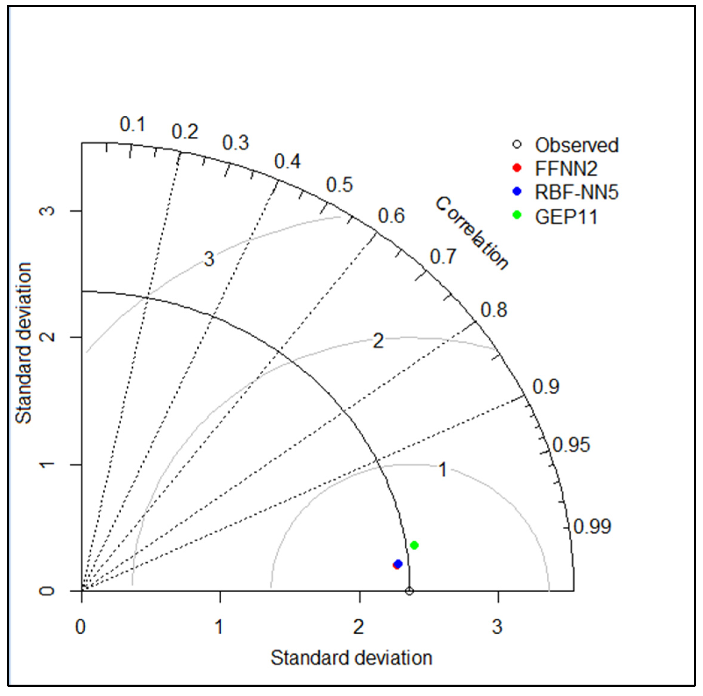
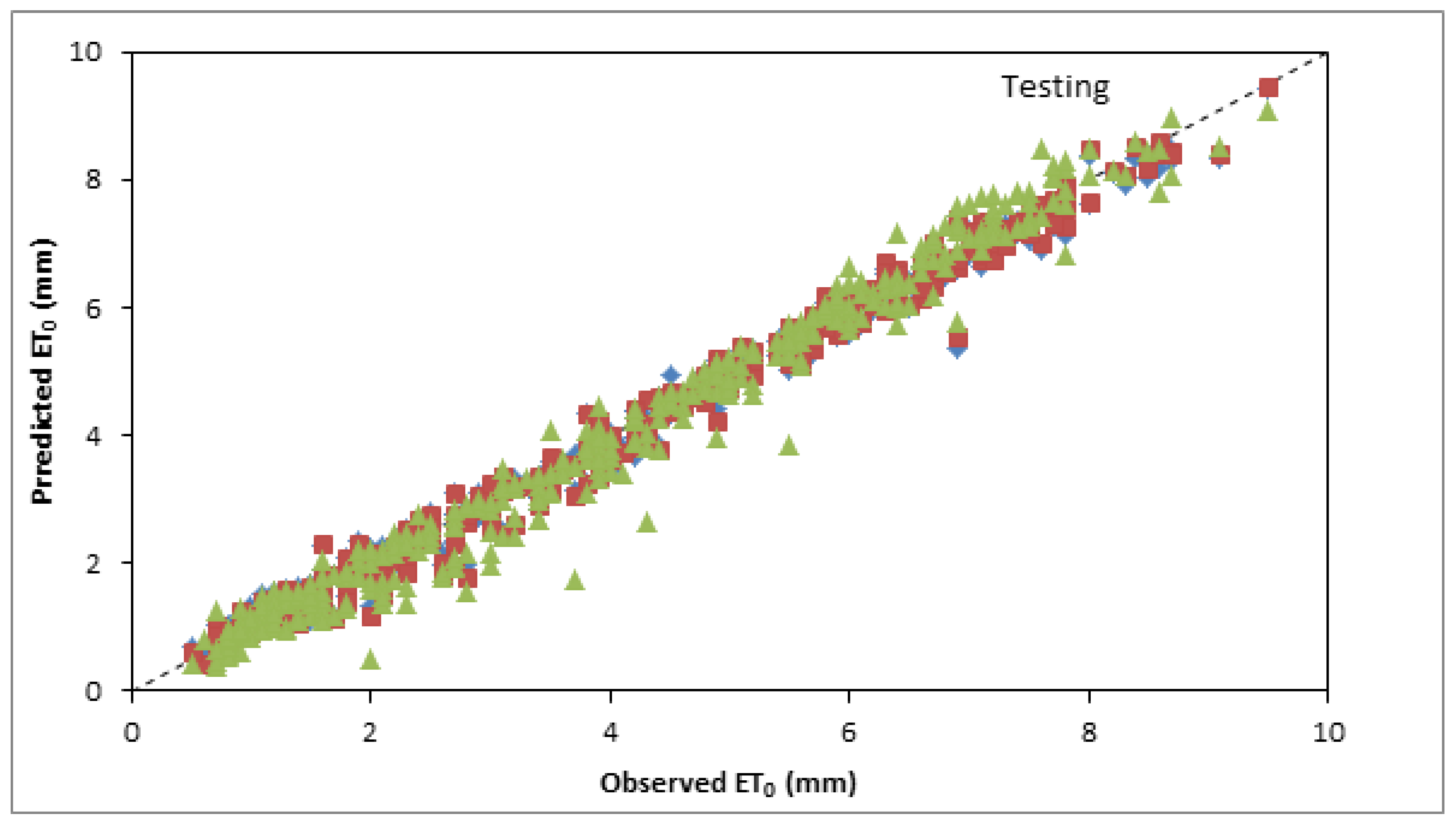
3.4. Inter Comparison among Best and Optimum Input Combination Based Models
4. Conclusions
Author Contributions
Funding
Data Availability Statement
Acknowledgments
Conflicts of Interest
References
- Gilbert, M.E.; Hernandez, M.I. How should crop water-use efficiency be analyzed? A warning about spurious correlations. Field Crops Res. 2019, 235, 59–67. [Google Scholar] [CrossRef]
- Ghiat, I.; Mackey, H.R.; Al-Ansari, T. A review of evapotranspiration measurement models, techniques and methods for open and closed agricultural field applications. Water 2021, 13, 2523. [Google Scholar] [CrossRef]
- Allen, R.; Peirera, L.S.; Raes, D.; Smith, M. Crop Evapotranspiration—Guidelines for Computing Crop Water Requirements; FAO—Food and Agriculture Organization of the United Nations: Rome, Italy, 1998; ISBN 92-5-104219-5. [Google Scholar]
- Sun, G.; Alstad, K.; Chen, J.; Chen, S.; Ford, C.R.; Lin, G.; Zhang, Z. A general predictive model for estimating monthly ecosystem evapotranspiration. Ecohydrology 2011, 4, 245–255. [Google Scholar] [CrossRef]
- Amatya, D.M.; Muwamba, A.; Panda, S.; Callahan, T.J.; Harder, S.; Pellett, C.A. Assessment of spatial and temporal variation of potential evapotranspiration estimated by four methods for South Carolina, USA. JSCWR 2018, 5, 3–24. [Google Scholar] [CrossRef] [Green Version]
- Yu, H.; Cao, C.; Zhang, Q.; Bao, Y. Construction of an evapotranspiration model and analysis of spatiotemporal variation in Xilin River Basin, China. PLoS ONE 2021, 16, e0256981. [Google Scholar] [CrossRef]
- Thornthwaite, C.W. An approach toward a national classification of climate. Geogr. Rev. 1948, 38, 55–94. [Google Scholar] [CrossRef]
- Blaney, H.F.; Criddle, W.D. Determining Water Requirements in Irrigated Areas from Climatological and Irrigation Data; US Soil Conservation Service: Washington, DC, USA, 1950.
- Makkink, G.F. Testing the Penman formula by means of lysimeters. J. Inst. Water Eng. 1957, 11, 277–288. [Google Scholar]
- Priestley, C.H.B.; Taylor, R.J. On the assessment of surface heat flux and evaporation using large-scale parameters. Mon. Weather Rev. 1972, 100, 81–92. [Google Scholar] [CrossRef]
- Hargreaves, G.H.; Samani, Z.A. Reference crop evapotranspiration from temperature. Appl. Eng. Agric. 1985, 1, 96–99. [Google Scholar] [CrossRef]
- Kumar, M.; Bandyopadhyay, A.; Raghuwanshi, N.S.; Singh, R. Comparative study of conventional and artificial neural network-based ET0 estimation models. Irrig. Sci. 2008, 26, 531–545. [Google Scholar] [CrossRef]
- Mohawesh, O.E. Artificial neural network for estimating monthly reference evapotranspiration under arid and semi-arid environments. Arch. Agron. Soil Sci. 2011, 59, 105–117. [Google Scholar] [CrossRef]
- Eslamian, S.S.; Gohari, S.A.; Zareian, M.J.; Firoozfar, A. Estimating Penman–Monteith reference evapotranspiration using artificial neural networks and genetic algorithm: A case study. Arab. J. Sci. Eng. 2012, 37, 935–944. [Google Scholar] [CrossRef]
- Citakoglu, H.; Cobaner, M.; Haktanir, T.; Kisi, O. Estimation of monthly mean reference evapotranspiration in Turkey. Water Resour. Manag. 2014, 28, 99–113. [Google Scholar] [CrossRef]
- Sattari, M.T.; Apaydin, H.; Shamshirband, S. Performance evaluation of deep learning-based gated recurrent units (GRUs) and tree-based models for estimating ET0 by using limited meteorological variables. Mathematics 2020, 8, 972. [Google Scholar] [CrossRef]
- Sattari, M.T.; Mirabbasi, R.; Sushab, R.S.; Abraham, J. Prediction of level in Ardebil plain using support vector regression and M5 tree model. Groundwater 2018, 56, 636–646. [Google Scholar] [CrossRef] [PubMed]
- Rouzegari, N.; Hassanzadeh, Y.; Sattari, M.T. Using the hybrid simulated annealing-M5 tree algorithms to extract the If-Then operation rules in a single reservoir. Water Resour. Manag. 2019, 33, 3655–3672. [Google Scholar] [CrossRef]
- Apaydin, H.; Feizi, H.; Sattari, M.T.; Colak, M.S.; Shamshirband, S.; Chau, K.-W. Comparative analysis of recurrent neural network architectures for reservoir inflow forecasting. Water 2020, 12, 1500. [Google Scholar] [CrossRef]
- Shabani, S.; Samadianfard, S.; Sattari, M.T.; Mosavi, A.; Shamshirband, S.; Kmet, T.; Várkonyi-Kóczy, A.R. Modeling pan evaporation using Gaussian process regression K-nearest neighbors random forest and support vector machines; Comparative analysis. Atmosphere 2020, 11, 66. [Google Scholar] [CrossRef] [Green Version]
- de Oliveira Ferreira Silva, C.; de Castro Teixeira, A.H.; Manzione, R.L. Agriwater: An R package for spatial modelling of energy balance and actual evapotranspiration using satellite images and agrometeorological data. Environ. Model. Softw. 2019, 120, 104497. [Google Scholar] [CrossRef]
- Thorp, K.R.; Marek, G.W.; DeJonge, K.C.; Evett, S.R.; Lascano, R.J. Novel methodology to evaluate and compare evapotranspiration algorithms in an agroecosystem model. Environ. Model. Softw. 2019, 119, 214–227. [Google Scholar] [CrossRef]
- Guven, A.; Aytek, A.; Yuce, M.I.; Aksoy, H. Genetic programming-based empirical model for daily reference evapotranspiration estimation. Clean Soil Air Water 2008, 36, 905–912. [Google Scholar] [CrossRef]
- Rahimikhoob, A. Estimation of evapotranspiration based on only air temperature data using artificial neural networks for a subtropical climate in Iran. Theor. Appl. Climatol. 2010, 101, 83–91. [Google Scholar] [CrossRef]
- Ozkan, C.; Kisi, O.; Akay, B. Neural networks with artificial bee colony algorithm for modeling daily reference evapotranspiration. Irrig. Sci. 2011, 29, 431–441. [Google Scholar] [CrossRef]
- Cobaner, M. Reference evapotranspiration based on Class A pan evaporation via wavelet regression technique. Irrig. Sci. 2013, 31, 119–134. [Google Scholar] [CrossRef]
- Ladlani, I.; Houichi, L.; Djemili, L.; Heddam, S.; Belouz, K. Estimation of daily reference evapotranspiration (ET0) in the North of Algeria using adaptive neuro-fuzzy inference system (ANFIS) and multiple linear regression (MLR) models: A comparative study. Arab. J. Sci. Eng. 2014, 39, 5959–5969. [Google Scholar] [CrossRef]
- Wen, X.; Si, J.; He, Z.; Wu, J.; Shao, H.; Yu, H. Support-vector-machine-based models for modeling daily reference evapotranspiration with limited climatic data in extreme arid regions. Water Resour. Manag. 2015, 29, 3195–3209. [Google Scholar] [CrossRef]
- Gocić, M.; Motamedi, S.; Shamshirband, S.; Petković, D.; Ch, S.; Hashim, R.; Arif, M. Soft computing approaches for forecasting reference evapotranspiration. Comput. Electron. Agric. 2015, 113, 164–173. [Google Scholar] [CrossRef]
- Petković, D.; Gocic, M.; Shamshirband, S.; Qasem, S.N.; Trajkovic, S. Particle swarm optimization-based radial basis function network for estimation of reference evapotranspiration. Theor. Appl. Climatol. 2016, 125, 555–563. [Google Scholar] [CrossRef]
- Pandey, P.K.; Nyori, T.; Pandey, V. Estimation of reference evapotranspiration using data driven techniques under limited data conditions. Model. Earth Syst. Environ. 2017, 3, 1449–1461. [Google Scholar] [CrossRef]
- Fan, J.; Yue, W.; Wu, L.; Zhang, F.; Cai, H.; Wang, X.; Lu, X.; Xiang, Y. Evaluation of SVM, ELM and four tree-based ensemble models for predicting daily reference evapotranspiration using limited meteorological data in different climates of China. Agric. For. Meteorol. 2018, 263, 225–241. [Google Scholar] [CrossRef]
- Wu, L.; Peng, Y.; Fan, J.; Wang, Y. Machine learning models for the estimation of monthly mean daily reference evapotranspiration based on cross-station and synthetic data. Hydrol. Res. 2019, 50, 1730–1750. [Google Scholar] [CrossRef]
- Douaoui, A.E.K.; Nicolas, H.; Walter, C. Detecting salinity hazards with in a semiarid context by means of combining soil and remote-sensing data. Geoderma 2006, 134, 217–230. [Google Scholar] [CrossRef]
- Shiri, J.; Kisi, Ö.; Anderas, G.; López, J.J.; Nazemi, A.H.; Stuyt, L.C.P.M. Daily reference evapotranspiration modeling by using genetic programming approach in the Basque Country (Northern Spain). J. Hydrol. 2012, 414, 302–316. [Google Scholar] [CrossRef]
- Leahy, P.; Kiely, G.; Corcoran, G. Structural optimization and input selection of an artificial neural network for river level prediction. J. Hydrol. 2008, 355, 192–201. [Google Scholar] [CrossRef]
- Ioannou, K.; Myronidis, D.; Lefakis, P.; Stathis, D. The use of artificial neural networks (ANNs) for the forecast of precipitation levels of Lake Doirani (N. Greece). Fresenius Environ. Bull. 2010, 19, 1921–1927. [Google Scholar]
- Haciismailoglu, M.C.; Kucuk, I.; Derebasi, N. Prediction of dynamic hysteresis loops of nano-crystalline cores. Expert Syst. Appl. 2009, 36, 2225–2227. [Google Scholar] [CrossRef]
- Lin, F.; Chen, L.H. A non-linear rainfall-runoff model using radial basis function network. J. Hydrol. 2004, 289, 1–8. [Google Scholar] [CrossRef]
- Wang, S.; Fu, Z.; Chen, H.; Nie, Y.; Wang, K. Modeling daily reference ET in the karst area of northwest Guangxi (China) using gene expression programming (GEP) and artificial neural network (ANN). Theor. Appl. Climatol. 2015, 126, 493–504. [Google Scholar] [CrossRef]
- Dubovský, V.; Dlouhá, D.; Pospíšil, L. The calibration of evaporation models against the Penman–Monteith equation on Lake Most. Sustainability 2020, 13, 313. [Google Scholar] [CrossRef]
- Myronidis, D.; Ivanova, E. Generating regional models for estimating the peak flows and environmental flows magnitude for the Bulgarian-Greek Rhodope mountain range torrential watersheds. Water 2020, 12, 784. [Google Scholar] [CrossRef] [Green Version]
- Han, X.; Wei, Z.; Zhang, B.; Li, Y.; Du, T.; Chen, H. Crop evapotranspiration prediction by considering dynamic change of crop coefficient and the precipitation effect in back-propagation neural network model. J. Hydrol. 2021, 596, 126104. [Google Scholar] [CrossRef]


| Name of Sensor | Measuring Unit |
|---|---|
| Psychrometer | % |
| Heliograph | Minute |
| Anemometer | 0.3 to 50 m/s |
| Wind direction | 0° to 360° |
| Pyranometer | 0…1400 W/m2 (Max 2000) |
| Albedometer | −2000 to 2000 W/m2 |
| Air temperature | −30 °C to 70 °C |
| Soil temperature | −50 °C to 50 °C |
| Evaporation pan | Mm of water |
| Rain gauge | Mm of water (resolution 0.1 mm) |
| Data Set | Unit | Xmin | Xmax | Xmean | Sx | CV (Sx/Xmean) |
|---|---|---|---|---|---|---|
| Tmin | °C | −4.30 | 26.29 | 11.68 | 6.87 | 0.59 |
| Tmax | °C | 6.98 | 48.16 | 27.28 | 8.89 | 0.33 |
| Tmean | °C | 3.87 | 37.23 | 19.48 | 7.53 | 0.39 |
| RH | % | 21.50 | 95.66 | 59.69 | 14.39 | 0.24 |
| WS | m/s | 0.00 | 28.94 | 6.66 | 3.81 | 0.57 |
| SD | h | 0.00 | 14.10 | 7.21 | 4.14 | 0.57 |
| GR | mm | 9.72 | 1791.04 | 969.52 | 446.08 | 0.46 |
| Parameter | Value |
|---|---|
| Hidden layer transfer Function | Tangent sigmoid transfer function (tansig) |
| Output layer transfer Function | Linear transfer function (purelin) |
| Training function | Levenberg-Marquardt |
| Maximum number of epochs to train | 1000 |
| Maximum validation failures | 6 |
| Minimum performance gradient | 1 × 10⁻⁷ |
| Initial mu | 0.001 |
| mu decrease factor | 0.1 |
| mu increase factor | 10 |
| Maximum mu | 1 × 10¹⁰ |
| Maximum time to train in seconds | Inf |
| Model | Input | Neurons | Training Phase | Testing Phase | ||||
|---|---|---|---|---|---|---|---|---|
| R2 | RMSE | EF | R2 | RMSE | EF | |||
| FFNN1 | Tmin, Tmax, Tmean, (Tmax − Tmin), RH, I, WS, GR | 18 | 0.9903 | 0.2338 | 0.9901 | 0.9918 | 0.2389 | 0.9898 |
| FFNN2 | Tmax, Tmean, (Tmax − Tmin), RH, I, WS, GR | 19 | 0.9903 | 0.2332 | 0.9902 | 0.9921 | 0.2342 | 0.9902 |
| FFNN3 | Tmin, Tmean, (Tmax − Tmin), RH, I, WS, GR | 13 | 0.9905 | 0.2308 | 0.9904 | 0.9917 | 0.2368 | 0.9900 |
| FFNN4 | Tmin, Tmax, (Tmax − Tmin), RH, I, WS, GR | 19 | 0.9903 | 0.2336 | 0.9901 | 0.9920 | 0.2378 | 0.9899 |
| FFNN5 | Tmin, Tmax, Tmean, RH, I, WS, GR | 11 | 0.9899 | 0.2376 | 0.9898 | 0.9916 | 0.2393 | 0.9897 |
| FFNN6 | Tmin, Tmax, Tmean, (Tmax − Tmin), I, WS, GR | 12 | 0.9782 | 0.3481 | 0.9781 | 0.9859 | 0.3102 | 0.9828 |
| FFNN7 | Tmin, Tmax, Tmean, (Tmax − Tmin), RH, WS, GR | 19 | 0.9883 | 0.2566 | 0.9881 | 0.9900 | 0.2536 | 0.9885 |
| FFNN8 | Tmin, Tmax, Tmean, (Tmax − Tmin), RH, I, GR | 14 | 0.9399 | 0.5799 | 0.9393 | 0.9603 | 0.5046 | 0.9544 |
| FFNN9 | Tmin, Tmax, Tmean, (Tmax − Tmin), RH, I, WS | 14 | 0.9676 | 0.4245 | 0.9675 | 0.9748 | 0.4032 | 0.9709 |
| FFNN10 | Tmean, RH, I, WS, GR | 16 | 0.9895 | 0.2435 | 0.9893 | 0.9907 | 0.2513 | 0.9887 |
| FFNN11 | Tmean, RH, WS, GR | 19 | 0.9875 | 0.2656 | 0.9873 | 0.9892 | 0.2623 | 0.9877 |
| FFNN12 | Tmean, RH, I, WS | 11 | 0.9672 | 0.4265 | 0.9671 | 0.9716 | 0.4124 | 0.9695 |
| FFNN13 | RH, I, WS, GR | 8 | 0.9217 | 0.6593 | 0.9215 | 0.9465 | 0.5533 | 0.9452 |
| FFNN14 | Tmean, RH, WS | 19 | 0.9172 | 0.6770 | 0.9172 | 0.9165 | 0.6845 | 0.9161 |
| FFNN15 | Tmean, RH | 14 | 0.8528 | 0.9047 | 0.8522 | 0.8966 | 0.7745 | 0.8926 |
| FFNN16 | Tmean, WS | 7 | 0.8326 | 0.9633 | 0.8324 | 0.8520 | 0.9224 | 0.8477 |
| FFNN17 | RH, WS | 20 | 0.7771 | 1.1120 | 0.7767 | 0.8439 | 0.9488 | 0.8388 |
| Model | Input Combination | Training Phase | Testing Phase | |||||
|---|---|---|---|---|---|---|---|---|
| Spread | R2 | RMSE | EF | R2 | RMSE | EF | ||
| RBF1 | Tmin, Tmax, Tmean, (Tmax − Tmin), RH, I, WS, GR | 1187.55 | 0.9911 | 0.2215 | 0.9911 | 0.9909 | 0.2406 | 0.9896 |
| RBF2 | Tmax, Tmean, (Tmax − Tmin), RH, I, WS, GR | 1187.55 | 0.9910 | 0.2238 | 0.9910 | 0.9910 | 0.2382 | 0.9898 |
| RBF3 | Tmin, Tmean, (Tmax − Tmin), RH, I, WS, GR | 1385.47 | 0.9906 | 0.2279 | 0.9906 | 0.9910 | 0.2377 | 0.9899 |
| RBF4 | Tmin, Tmax, (Tmax − Tmin), RH, I, WS, GR | 1385.47 | 0.9907 | 0.2265 | 0.9907 | 0.9910 | 0.2378 | 0.9899 |
| RBF5 | Tmin, Tmax, Tmean, RH, I, WS, GR | 1385.47 | 0.9907 | 0.2270 | 0.9907 | 0.9911 | 0.2374 | 0.9899 |
| RBF6 | Tmin, Tmax, Tmean, (Tmax − Tmin), I, WS, GR | 791.70 | 0.9805 | 0.3284 | 0.9805 | 0.9842 | 0.3216 | 0.9815 |
| RBF7 | Tmin, Tmax, Tmean, (Tmax − Tmin), RH, WS, GR | 1187.55 | 0.9890 | 0.2466 | 0.9890 | 0.9901 | 0.2445 | 0.9893 |
| RBF8 | Tmin, Tmax, Tmean, (Tmax − Tmin), RH, I, GR | 593.77 | 0.9456 | 0.5489 | 0.9456 | 0.9549 | 0.5076 | 0.9539 |
| RBF9 | Tmin, Tmax, Tmean, (Tmax − Tmin), RH, I, WS | 1781.32 | 0.9753 | 0.3696 | 0.9753 | 0.9616 | 0.4729 | 0.9600 |
| RBF10 | Tmean, RH, I, WS, GR | 791.70 | 0.9907 | 0.2267 | 0.9907 | 0.9901 | 0.2530 | 0.9885 |
| RBF11 | Tmean, RH, WS, GR | 593.77 | 0.9886 | 0.2514 | 0.9886 | 0.9892 | 0.2551 | 0.9884 |
| RBF12 | Tmean, RH, I, WS | 1583.40 | 0.9704 | 0.4047 | 0.9704 | 0.9699 | 0.4298 | 0.9669 |
| RBF13 | RH, I, WS, GR | 593.77 | 0.9300 | 0.6224 | 0.9300 | 0.9400 | 0.5873 | 0.9382 |
| RBF14 | Tmean, RH, WS | 1385.47 | 0.9214 | 0.6599 | 0.9214 | 0.9140 | 0.6941 | 0.9137 |
| RBF15 | Tmean, RH | 791.70 | 0.8569 | 0.8902 | 0.8569 | 0.8915 | 0.7834 | 0.8901 |
| RBF16 | Tmean, WS | 791.70 | 0.8400 | 0.9413 | 0.8400 | 0.8480 | 0.9279 | 0.8458 |
| RBF17 | RH, WS | 791.70 | 0.7779 | 1.1089 | 0.7779 | 0.8434 | 0.9441 | 0.8404 |
| Parameter | Value |
|---|---|
| Number of chromosomes | 30 |
| Head size | 8 |
| Number of genes | 3 |
| Linking function | Addition |
| Fitness function error type | RMSE |
| Mutation rate | 0.044 |
| Inversion rate | 0.1 |
| IS transposition | 0.1 |
| RIS transposition | 0.1 |
| One-point recombination rate | 0.3 |
| wo-point recombination rate | 0.3 |
| Gene recombination rate | 0.1 |
| Gene transposition rate | 0.1 |
| Model | Input Combination | Training Phase | Testing Phase | ||||
|---|---|---|---|---|---|---|---|
| R2 | RMSE | EF | R2 | RMSE | EF | ||
| GEP1 | Tmin, Tmax, Tmean, (Tmax − Tmin), RH, I, WS, GR | 0.8959 | 0.7732 | 0.8920 | 0.9190 | 0.6945 | 0.9136 |
| GEP2 | Tmax, Tmean, (Tmax − Tmin), RH, I, WS, GR | 0.9075 | 0.7227 | 0.9057 | 0.9323 | 0.6251 | 0.9300 |
| GEP3 | Tmin, Tmean, (Tmax − Tmin), RH, I, WS, GR | 0.9026 | 0.7361 | 0.9021 | 0.9300 | 0.6652 | 0.9208 |
| GEP4 | Tmin, Tmax, (Tmax − Tmin), RH, I, WS, GR | 0.8355 | 0.9692 | 0.8303 | 0.8627 | 0.9407 | 0.8416 |
| GEP5 | Tmin, Tmax, Tmean, RH, I, WS, GR | 0.8415 | 0.9721 | 0.8294 | 0.9033 | 0.8151 | 0.8810 |
| GEP6 | Tmin, Tmax, Tmean, (Tmax − Tmin), I, WS, GR | 0.9393 | 0.5804 | 0.9392 | 0.9629 | 0.4687 | 0.9607 |
| GEP7 | Tmin, Tmax, Tmean, (Tmax − Tmin), RH, WS, GR | 0.9664 | 0.4323 | 0.9663 | 0.9762 | 0.3795 | 0.9742 |
| GEP8 | Tmin, Tmax, Tmean, (Tmax − Tmin), RH, I, GR | 0.8636 | 0.8695 | 0.8635 | 0.9194 | 0.6925 | 0.9141 |
| GEP9 | Tmin, Tmax, Tmean, (Tmax − Tmin), RH, I, WS | 0.9353 | 0.6081 | 0.9332 | 0.9537 | 0.5604 | 0.9438 |
| GEP10 | Tmean, RH, I, WS, GR | 0.9085 | 0.7138 | 0.9080 | 0.9275 | 0.6435 | 0.9258 |
| GEP11 | Tmean, RH, WS, GR | 0.9606 | 0.4830 | 0.9579 | 0.9775 | 0.3701 | 0.9755 |
| GEP12 | Tmean, RH, I, WS | 0.9420 | 0.5885 | 0.9374 | 0.9597 | 0.5045 | 0.9544 |
| GEP13 | RH, I, WS, GR | 0.8560 | 0.9004 | 0.8536 | 0.9236 | 0.7069 | 0.9105 |
| GEP14 | Tmean, RH, WS | 0.8388 | 0.9563 | 0.8349 | 0.8797 | 0.8406 | 0.8735 |
| GEP15 | Tmean, RH | 0.8136 | 1.0598 | 0.7972 | 0.8635 | 0.9331 | 0.8441 |
| GEP16 | Tmean, WS | 0.7769 | 1.1312 | 0.7689 | 0.8057 | 1.0588 | 0.7993 |
| GEP17 | RH, WS | 0.6973 | 1.3112 | 0.6895 | 0.8062 | 1.1224 | 0.7744 |
| Model | Training Phase | Testing Phase | ||||
|---|---|---|---|---|---|---|
| R2 | RMSE | E | R2 | RMSE | E | |
| FFNN2 | 0.9903 | 0.2332 | 0.9902 | 0.9921 | 0.2342 | 0.9902 |
| RBFNN5 | 0.9907 | 0.2270 | 0.9907 | 0.9911 | 0.2374 | 0.9899 |
| GEP11 | 0.9606 | 0.4830 | 0.9579 | 0.9775 | 0.3701 | 0.9755 |
| Source of Variation | F | p-Value | Fcrit | Variation among Groups |
|---|---|---|---|---|
| Actual-FFNN2 | 0.171751 | 0.678682 | 3.854264 | Insignificant |
| Actual-RBFNN5 | 0.101036 | 0.750681 | 3.854264 | Insignificant |
| Actual-GEP11 | 0.126406 | 0.72229 | 3.854264 | Insignificant |
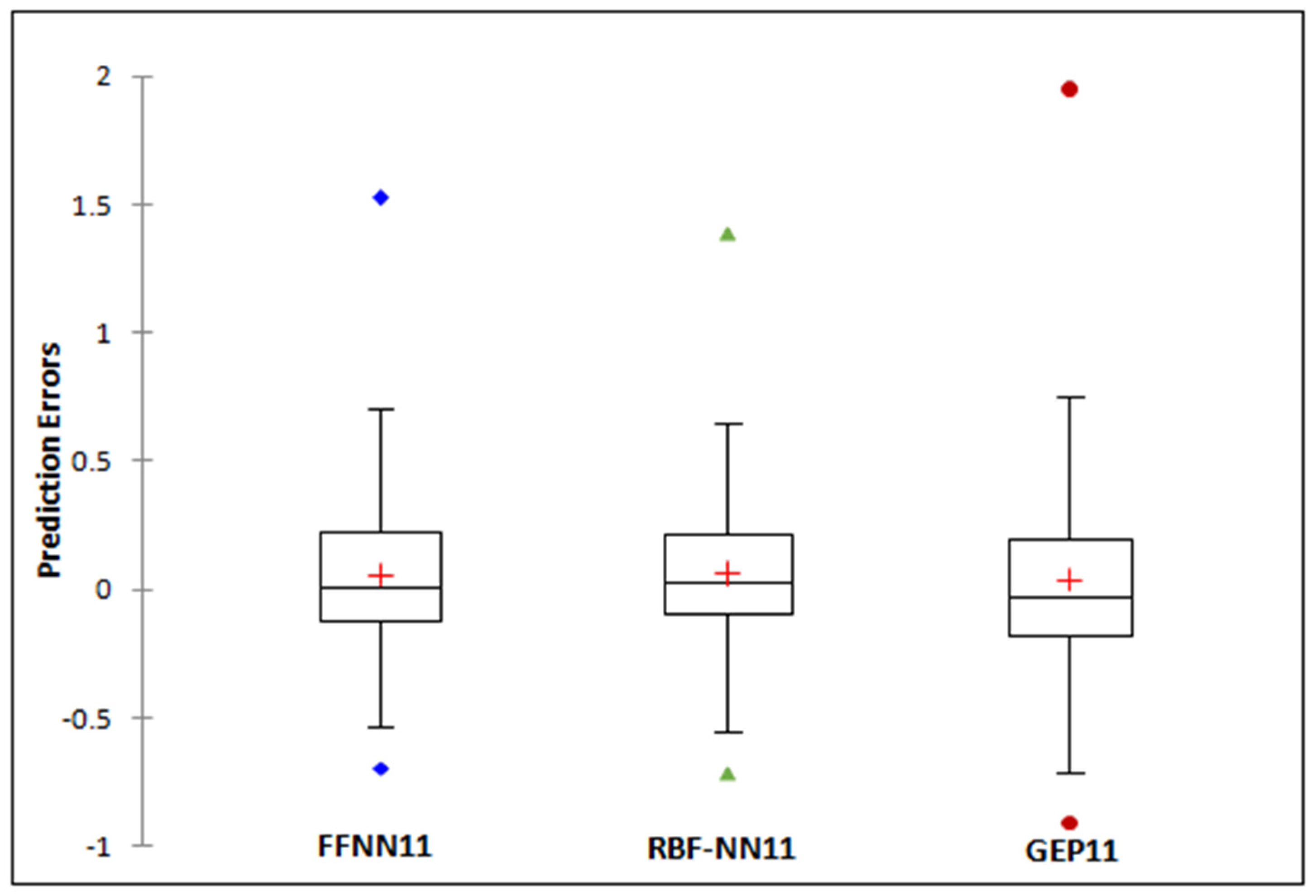
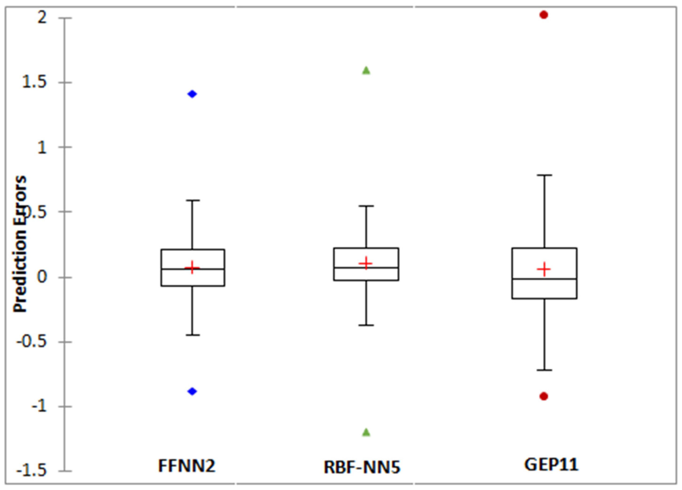
| Statistic | FFNN2 | RBFNN5 | GEP11 |
|---|---|---|---|
| Minimum | −0.8840 | −1.2231 | −0.8671 |
| Maximum | 1.4199 | 1.5204 | 1.9343 |
| 1st quartile | −0.0681 | −0.0726 | −0.1503 |
| Median | 0.0606 | 0.0250 | −0.0055 |
| 3rd quartile | 0.2091 | 0.1742 | 0.2176 |
| Mean | 0.0713 | 0.0548 | 0.0630 |
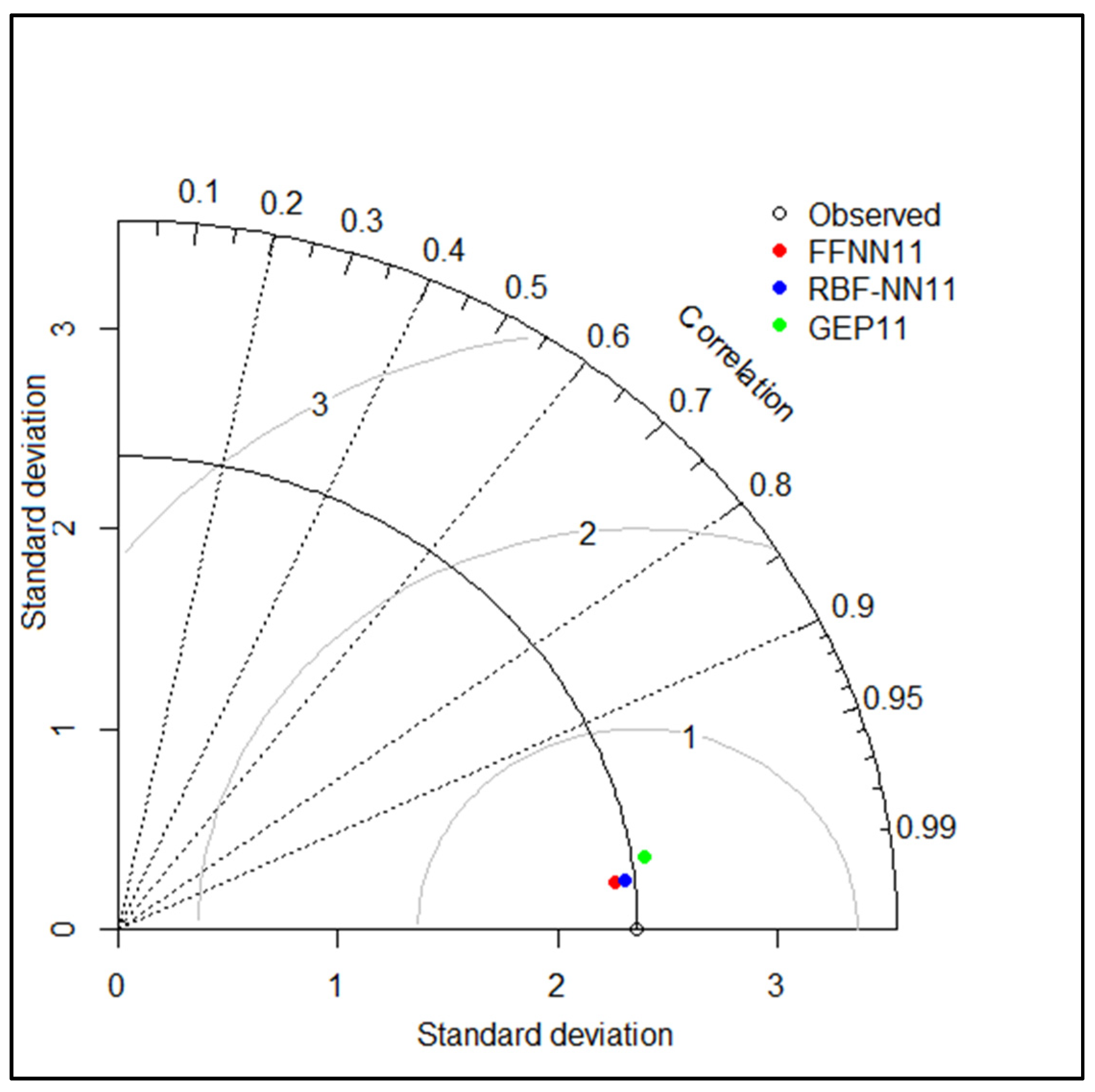
| Model | Training Phase | Testing Phase | ||||
|---|---|---|---|---|---|---|
| R2 | RMSE | E | R2 | RMSE | E | |
| FFNN | 0.9875 | 0.2656 | 0.9873 | 0.9892 | 0.2623 | 0.9877 |
| RBF | 0.9886 | 0.2514 | 0.9886 | 0.9892 | 0.2551 | 0.9884 |
| GEP | 0.9606 | 0.4830 | 0.9579 | 0.9775 | 0.3701 | 0.9755 |
| Source of Variation | F | p-Value | Fcrit | Variation among Groups |
|---|---|---|---|---|
| Observed-FFNN11 | 0.101466 | 0.750169 | 3.854264 | Insignificant |
| Observed-RBFNN11 | 0.119424 | 0.72976 | 3.854264 | Insignificant |
| Observed-GEP11 | 0.126406 | 0.72229 | 3.854264 | Insignificant |
| Statistic | FFNN11 | RBFNN11 | GEP11 |
|---|---|---|---|
| Minimum | −0.6918 | −0.7073 | −0.8671 |
| Maximum | 1.5230 | 1.3700 | 1.9343 |
| 1st Quartile | −0.1227 | −0.0952 | −0.1503 |
| Median | 0.0119 | 0.0221 | −0.0055 |
| 3rd Quartile | 0.2228 | 0.2111 | 0.2176 |
| Mean | 0.0548 | 0.0599 | 0.0630 |
Publisher’s Note: MDPI stays neutral with regard to jurisdictional claims in published maps and institutional affiliations. |
© 2022 by the authors. Licensee MDPI, Basel, Switzerland. This article is an open access article distributed under the terms and conditions of the Creative Commons Attribution (CC BY) license (https://creativecommons.org/licenses/by/4.0/).
Share and Cite
Achite, M.; Jehanzaib, M.; Sattari, M.T.; Toubal, A.K.; Elshaboury, N.; Wałęga, A.; Krakauer, N.; Yoo, J.-Y.; Kim, T.-W. Modern Techniques to Modeling Reference Evapotranspiration in a Semiarid Area Based on ANN and GEP Models. Water 2022, 14, 1210. https://doi.org/10.3390/w14081210
Achite M, Jehanzaib M, Sattari MT, Toubal AK, Elshaboury N, Wałęga A, Krakauer N, Yoo J-Y, Kim T-W. Modern Techniques to Modeling Reference Evapotranspiration in a Semiarid Area Based on ANN and GEP Models. Water. 2022; 14(8):1210. https://doi.org/10.3390/w14081210
Chicago/Turabian StyleAchite, Mohammed, Muhammad Jehanzaib, Mohammad Taghi Sattari, Abderrezak Kamel Toubal, Nehal Elshaboury, Andrzej Wałęga, Nir Krakauer, Ji-Young Yoo, and Tae-Woong Kim. 2022. "Modern Techniques to Modeling Reference Evapotranspiration in a Semiarid Area Based on ANN and GEP Models" Water 14, no. 8: 1210. https://doi.org/10.3390/w14081210