
Design of Groundwater Level Monitoring Networks for Maximum Data Acquisition at Minimum Travel Cost


 , , and
Abstract
:1. Introduction
2. Materials and Methods
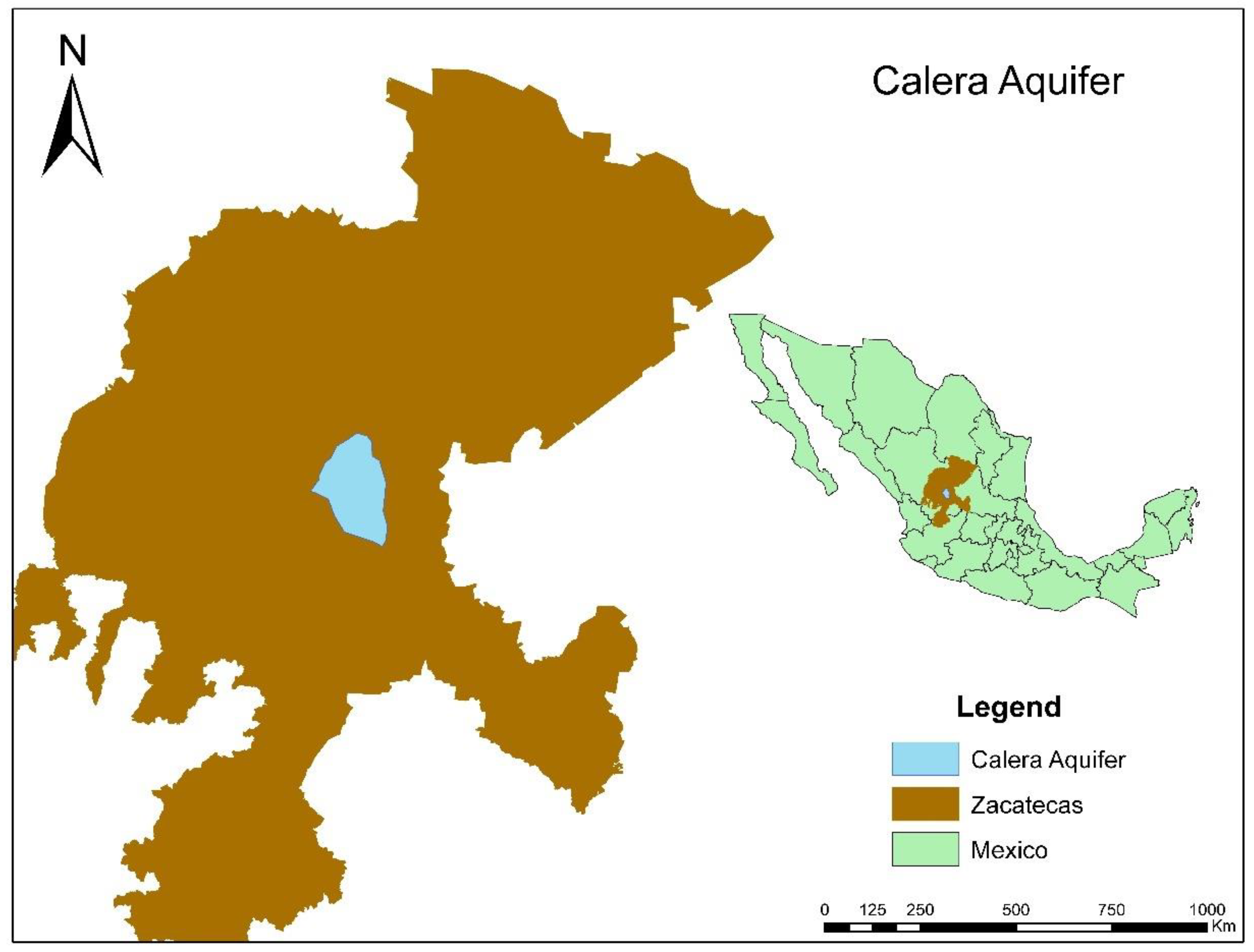
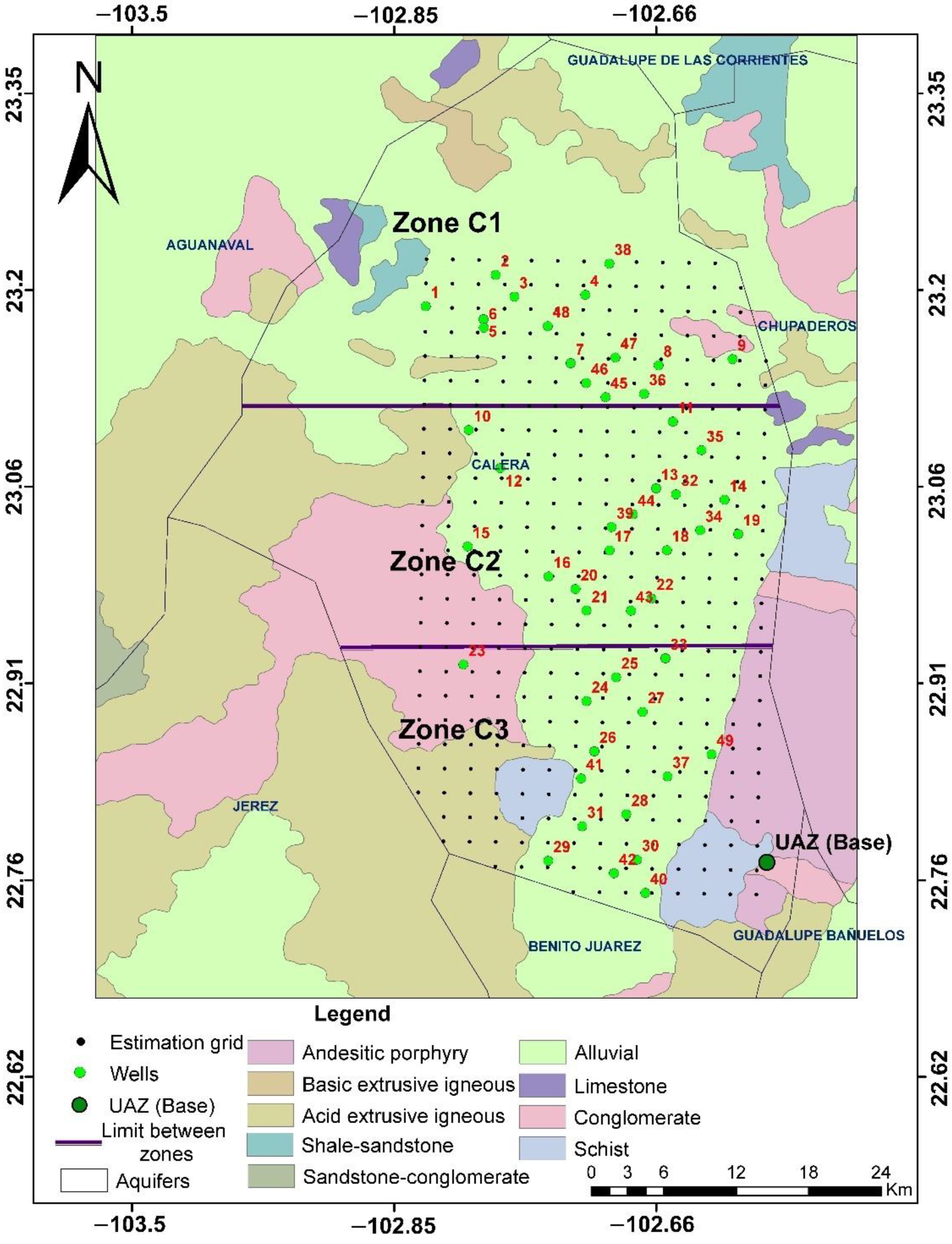
2.1. Location of the Study Area
2.1.1. Existing Groundwater-Level Monitoring Network
2.1.2. Estimation Grid and Monitoring Zones
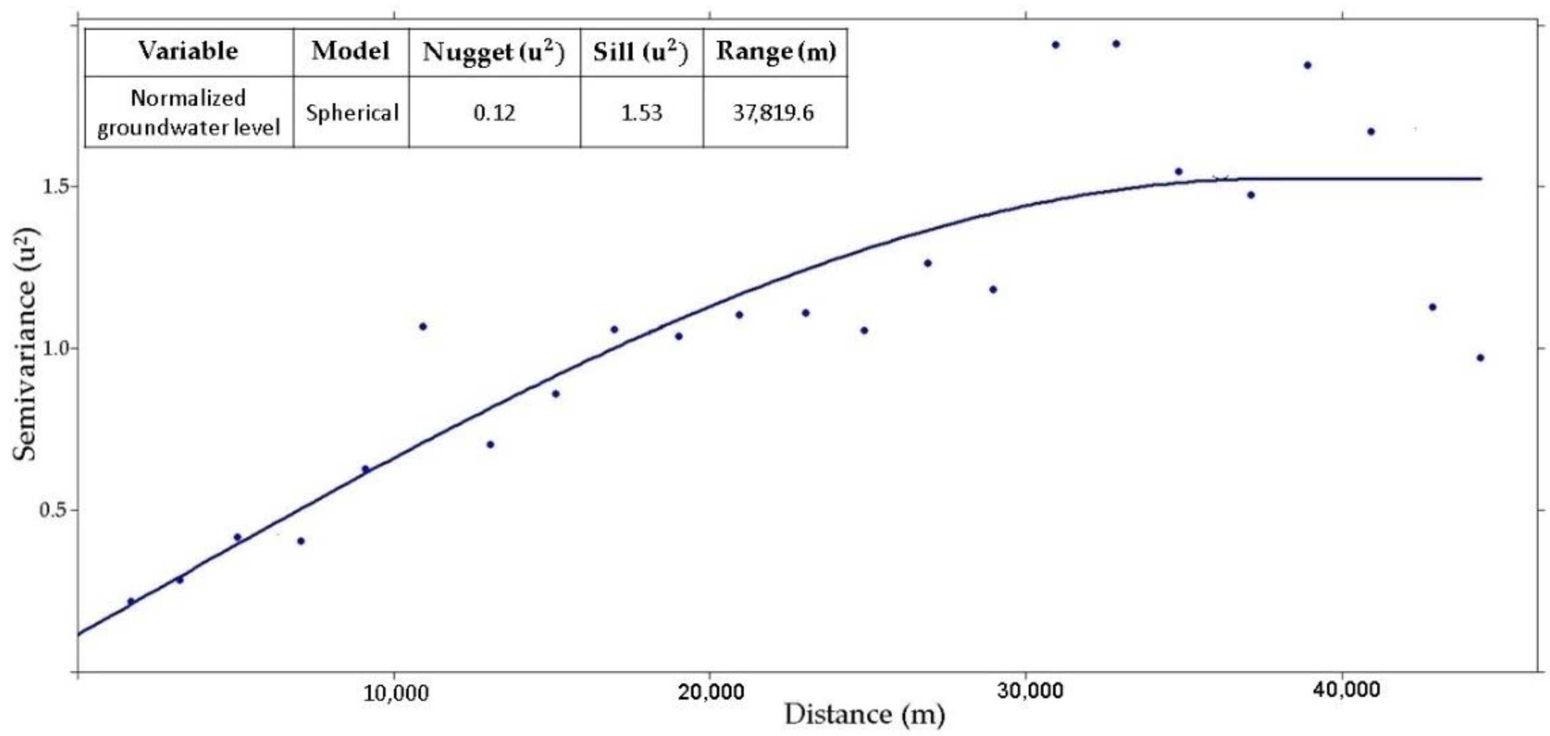
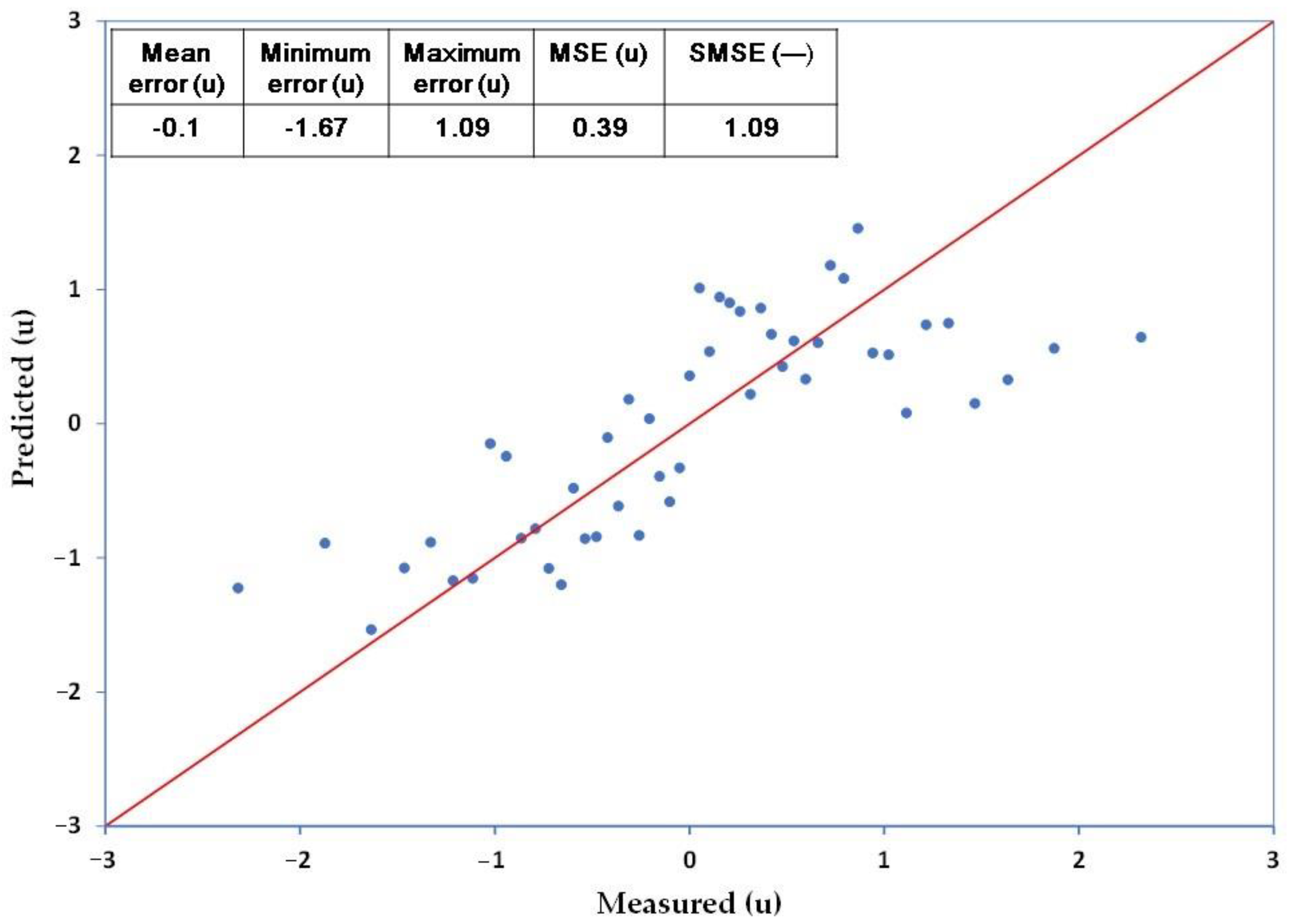
2.2. Geostatistical Analysis
2.3. Kalman Filter
2.4. Traveling Salesman Problem (TSP)
Branch and Bound
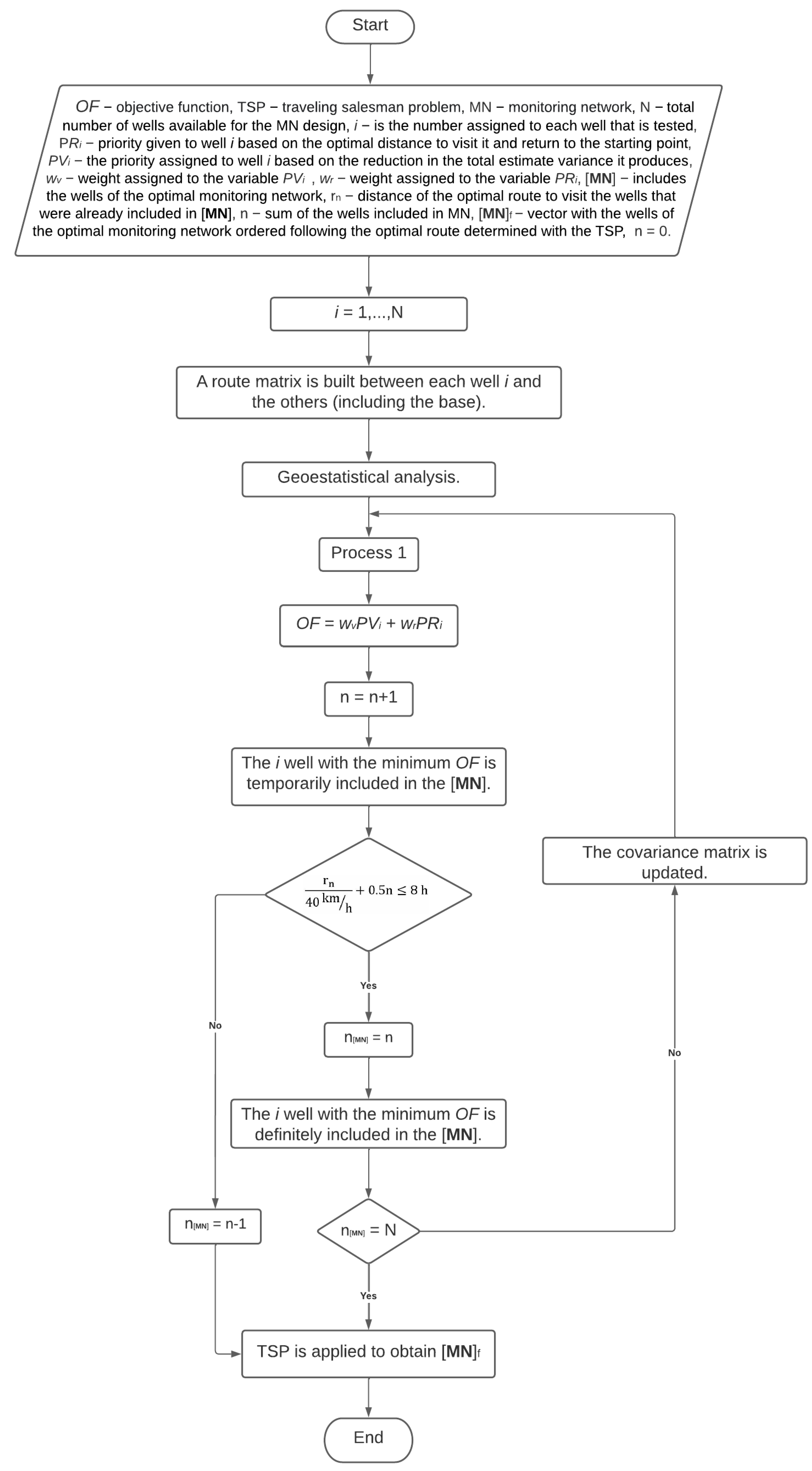
2.5. Objective Function for the Design of the Monitoring Network
- For each well that is not yet part of the [MN], the TSP is applied (including the previously selected wells) to compute the optimal route (ri) from the starting point and back.
- A is assigned to each well that is not part of the [MN], for the well with minimum ri, for the i well with maximum ri.
- A is assigned to each well that is not part of the [MN] following the Júnez-Ferreira method [31]; for the well that produces the largest reduction in the total estimate error variance, and for the well that was last selected.
3. Results and Discussions
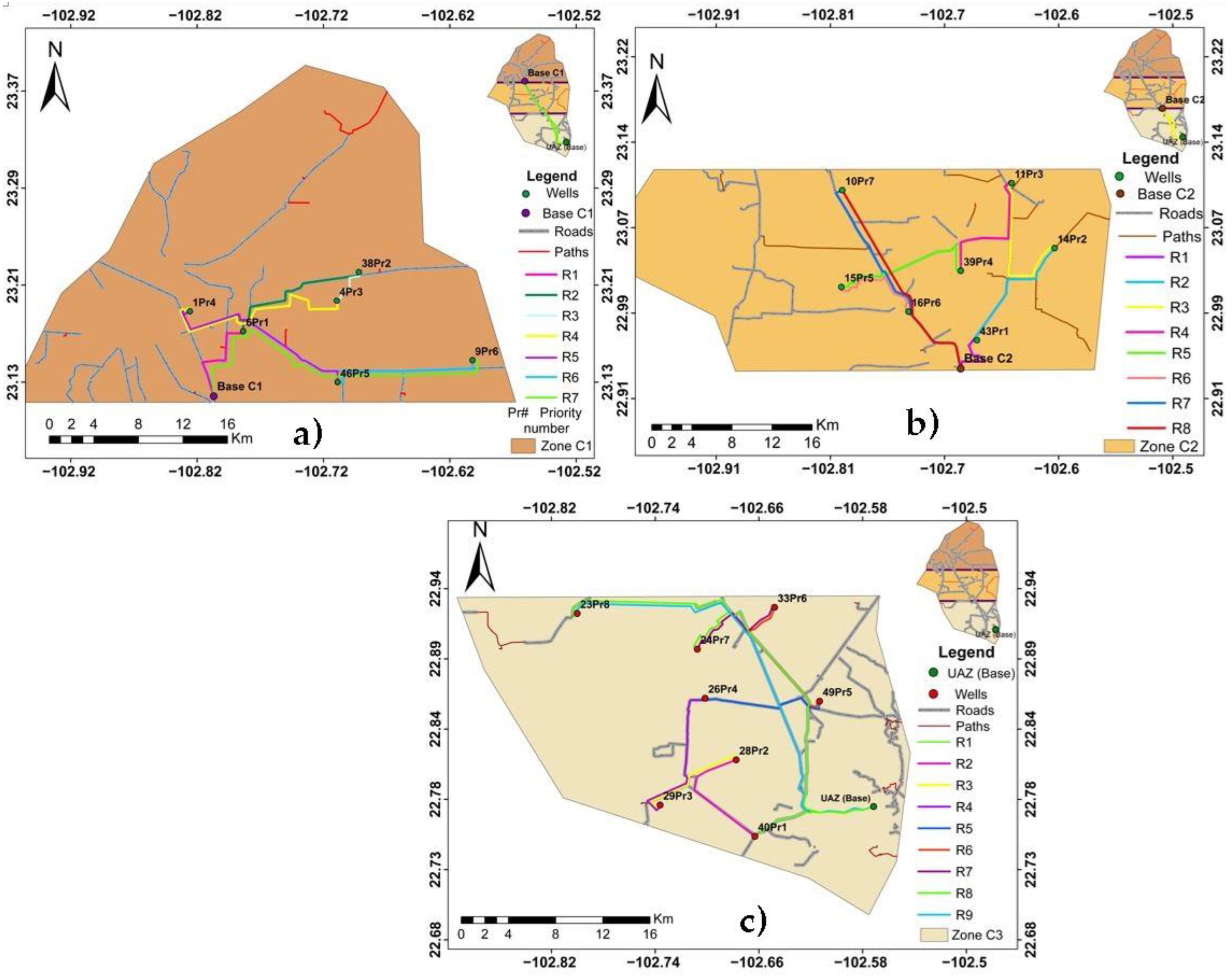
3.1. Monitoring Network Optimization
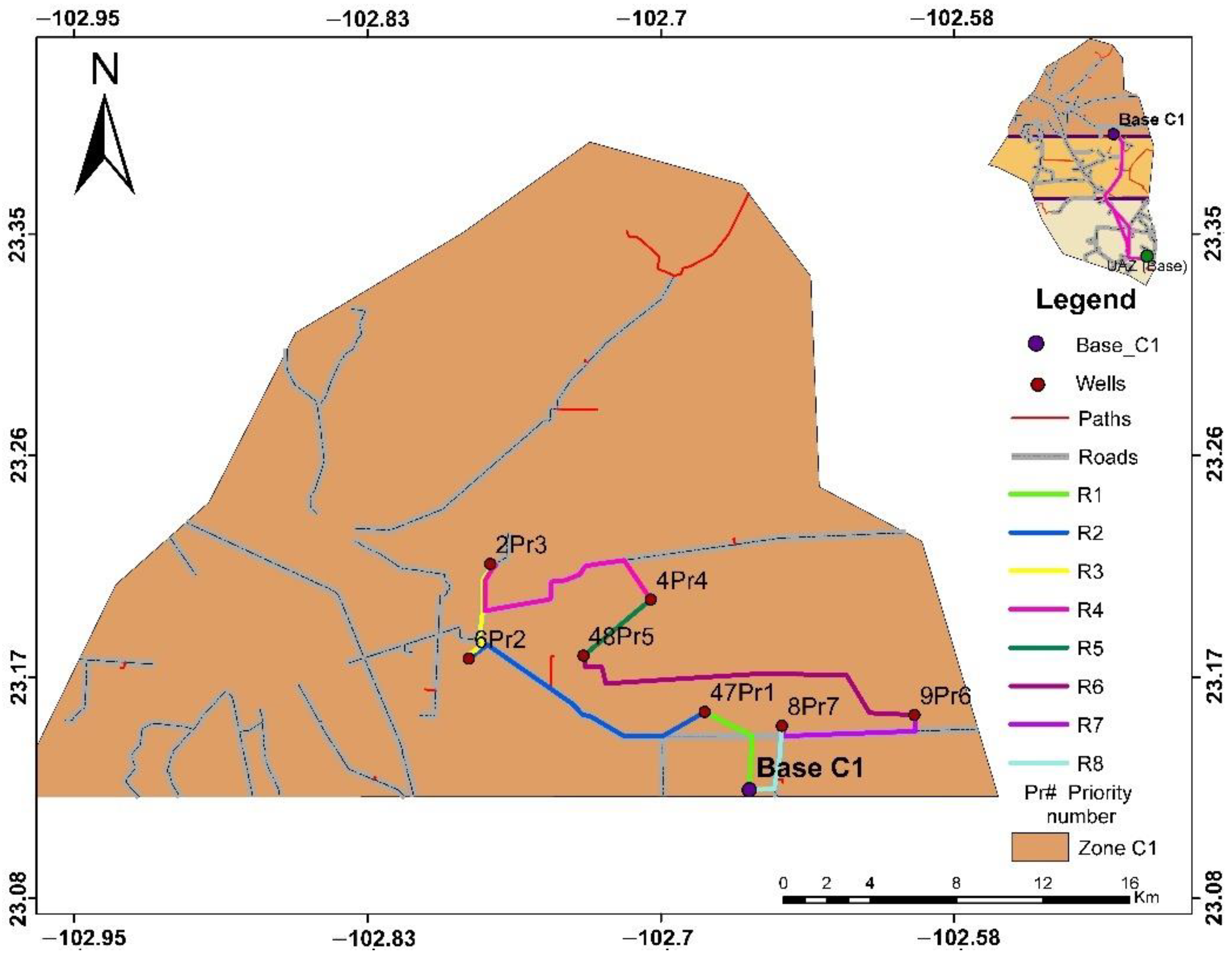
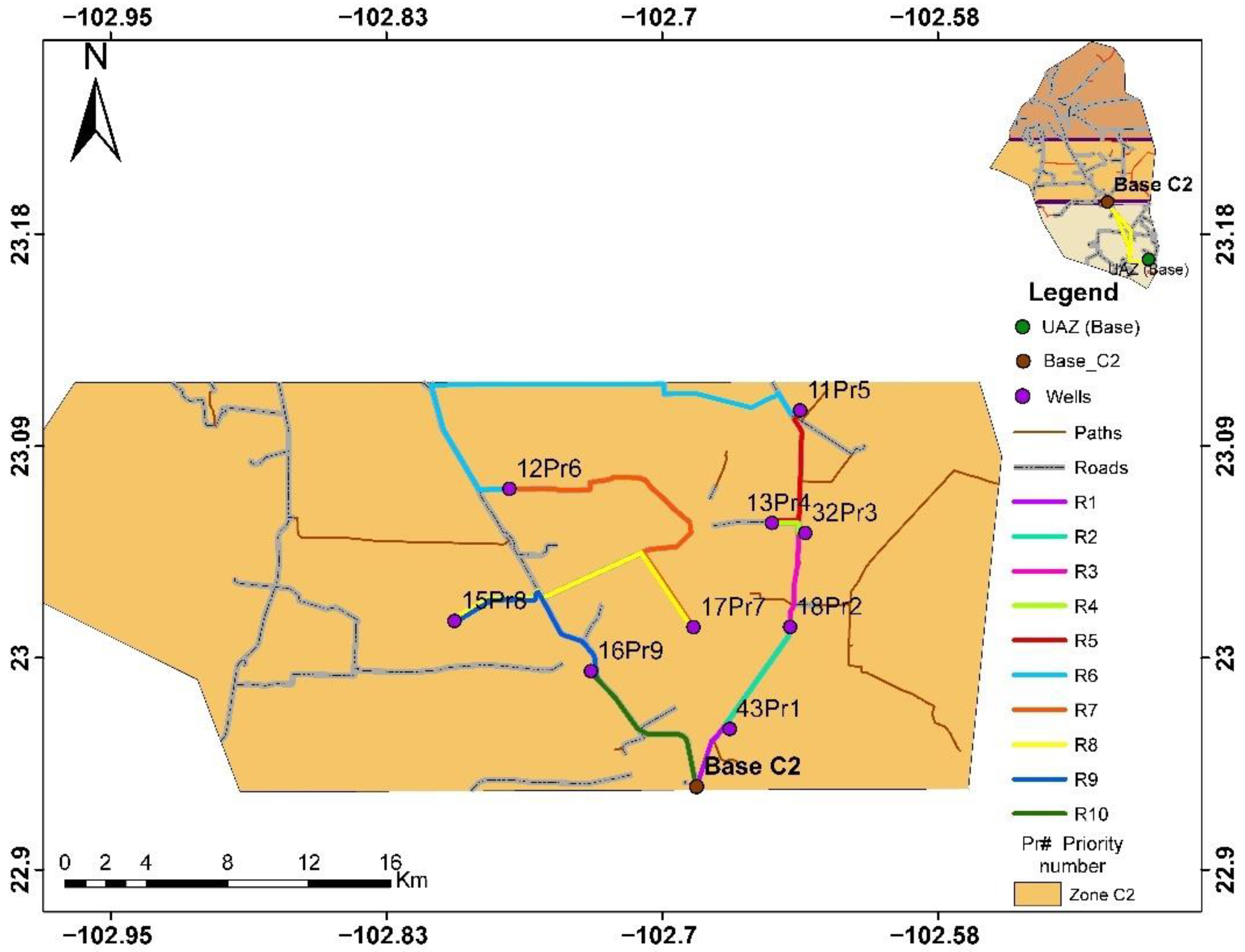
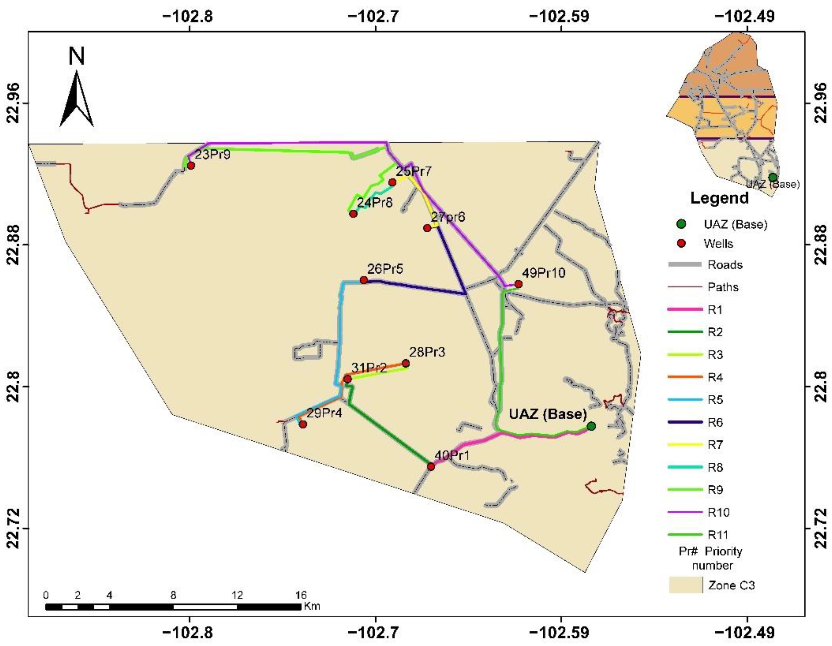
Monitoring Schemes for Zones C1, C2 and C3
4. Conclusions
Author Contributions
Funding
Data Availability Statement
Acknowledgments
Conflicts of Interest
Appendix A

| Well Number | Well Name | UTM X | UTM Y | Water Level (masl) |
|---|---|---|---|---|
| 1 | N-5 | 722,350.43 | 2,566,447.24 | 2193.86 |
| 2 | N-6 | 727,635.07 | 2,569,112.14 | 2071.40 |
| 3 | N-6′ | 729,084.62 | 2,567,334.11 | 2049.09 |
| 4 | S/N | 734,491.45 | 2,567,581.45 | 2046.78 |
| 5 | N-9 | 726,766.72 | 2,565,433.71 | 2082.56 |
| 6 | N-11 | 726,794.37 | 2,564,738.64 | 2179.70 |
| 7 | N-12 | 733,473.68 | 2,561,912.06 | 2015.18 |
| 8 | N-13 | 740,173.85 | 2,561,855.34 | 2042.99 |
| 9 | N-14 | 745,805.00 | 2,562,445.68 | 2061.46 |
| 10 | N-16 | 725,781.34 | 2,556,285.20 | 2045.21 |
| 11 | N-19 | 741,341.57 | 2,557,223.85 | 2033.42 |
| 12 | N-22 | 728,225.67 | 2,553,180.33 | 2021.23 |
| 13 | N-23 | 740,152.13 | 2,551,689.60 | 2018.38 |
| 14 | N-24 | 745,389.30 | 2,550,835.77 | 2014.00 |
| 15 | N-25 | 725,838.04 | 2,546,666.41 | 2150.80 |
| 16 | N-26 | 732,058.87 | 2,544,305.51 | 2146.40 |
| 17 | N-27 | 736,679.40 | 2546,528.74 | 2046.46 |
| 18 | N-28 | 741,053.95 | 2,546,610.64 | 2058.50 |
| 19 | N-30 A | 746,475.09 | 2,548,025.16 | 2034.61 |
| 20 | N-30 C | 734,125.96 | 2,543,297.39 | 2120.39 |
| 21 | N-31 | 734,994.10 | 2,541,532.17 | 2103.91 |
| 22 | N-33 | 739,935.57 | 2,542,607.28 | 2089.70 |
| 23 | SUST. | 725,659.20 | 2,536,936.50 | 2088.52 |
| 24 | N-35′ | 735,102.00 | 2,534,064.90 | 2100.25 |
| 25 | N-37 | 737,337.29 | 2,536,060.23 | 2103.44 |
| 26 | S/N | 735,770.90 | 2,529,933.11 | 2183.58 |
| 27 | S/N | 739,406.11 | 2,533,240.06 | 2099.34 |
| 28 | N-41 | 738,287.73 | 2,524,768.56 | 2155.56 |
| 29 | N-42 | 732,387.85 | 2,520,864.15 | 2141.80 |
| 30 | S/N | 739,167.82 | 2,521,061.75 | 2135.57 |
| 31 | C.P 4 | 734,931.70 | 2,523,728.33 | 2088.81 |
| 32 | SN RAFAEL | 741,669.08 | 2,551,221.58 | 2010.96 |
| 33 | S/N | 741,082.87 | 2,537,692.27 | 2080.30 |
| 34 | S/N | 743,570.81 | 2,548,288.58 | 2039.11 |
| 35 | S/N | 743,557.28 | 2,554,902.28 | 2037.05 |
| 36 | TALANCON | 739,107.71 | 2,559,477.68 | 2037.95 |
| 37 | N-15 | 741,398.13 | 2,527,950.69 | 2138.17 |
| 38 | VIVERO | 736,282.30 | 2,570,173.41 | 2030.83 |
| 39 | S/N | 736,794.51 | 2,548,441.69 | 2070.49 |
| 40 | S/N | 739,850.11 | 2,518,333.57 | 2128.86 |
| 41 | S/N | 734,796.27 | 2,527,680.68 | 2073.10 |
| 42 | S/N | 737,430.66 | 2,519,920.46 | 2160.77 |
| 43 | S/N | 738,393.26 | 2,541,570.25 | 2113.20 |
| 44 | S/N | 738,409.40 | 2,549,529.02 | 2046.07 |
| 45 | S/N | 736,172.37 | 2,559,163.21 | 1988.44 |
| 46 | S/N | 734,674.42 | 2,560,296.74 | 2011.40 |
| 47 | S/N | 736,874.70 | 2,562,436.55 | 2011.59 |
| 48 | S/N | 731,673.45 | 2,564,949.14 | 2038.76 |
| 49 | JESUS LOPEZ | 744,739.46 | 2,529,823.22 | 2272.53 |
References
- CONAGUA-AAM. Available online: http://sina.conagua.gob.mx/publicaciones/AAM_2018.pdf (accessed on 24 August 2021).
- Food and Agriculture Organization (FAO). Available online: https://www.fao.org/aquastat/es/overview/methodology/water-use (accessed on 8 September 2021).
- CONAGUA-EAM. Available online: http://sina.conagua.gob.mx/publicaciones/EAM_2018.pdf (accessed on 23 August 2021).
- Bhat, S.; Motz, L.H.; Pathak, C.; Kuebler, L. Geostatistics-based groundwater-level monitoring network design and its application to the Upper Floridan aquifer, USA. Environ. Monit. Assess. 2015, 187, 4183. [Google Scholar] [CrossRef] [PubMed]
- Molinari, A.; Guadagnini, L.; Marcaccio, M.; Guadagnini, A. Geostatistical multimodel approach for the assessment of the spatial distribution of natural background concentrations in large-scale groundwater bodies. Water Res. 2019, 149, 522–532. [Google Scholar] [CrossRef] [PubMed] [Green Version]
- Ahmadi, S.H.; Sedghamiz, A. Geostatistical Analysis of Spatial and Temporal Variations of Groundwater Level. Environ. Monit. Assess. 2007, 129, 277–294. [Google Scholar] [CrossRef] [PubMed]
- International Groundwater Resources Assessment Centre (IGRAC). Available online: https://www.un-igrac.org/sites/default/files/resources/files/GGMN%20Brochure%202016.pdf (accessed on 3 November 2021).
- Briseño-Ruiz, J.-V.; Júnez-Ferreira, H.-E.; Herrera-Zamarrón, G.-S. Method for the optimal design of networks to monitor groundwater levels. Water Technol. Sci. 2011, 2, 77–96. [Google Scholar]
- Kumari, K.; Jain, S.; Dhar, A. Computationally efficient approach for identification of fuzzy dynamic groundwater sampling network. Environ. Monit. Assess. 2019, 191, 310. [Google Scholar] [CrossRef]
- Mirzaie-Nodoushan, F.; Bozorg-Haddad, O.; Loáiciga, H.A. Optimal design of groundwater-level monitoring networks. J. Hydroinform. 2017, 19, 920–929. [Google Scholar] [CrossRef]
- Soltani, S.; Kordestani, M.; Karim Aghaee, P. New estimation methodologies for well logging problems via a combination of fuzzy Kalman filter and different smoothers. J. Pet. Sci. Eng. 2016, 145, 704–710. [Google Scholar] [CrossRef]
- Bierkens, M.F.; Knotters, M.; Hoogland, T. Space-time modeling of water table depth using a regionalized time series model and the Kalman filter. Water Res. 2001, 37, 1277–1290. [Google Scholar] [CrossRef]
- Luo, Q.; Wu, J.; Yang, Y.; Qian, J.; Wu, J. Multi-objective optimization of long-term groundwater monitoring network design using a probabilistic Pareto genetic algorithm under uncertainty. J. Hydrol. 2016, 534, 352–363. [Google Scholar] [CrossRef]
- Farlin, J.; Gallé, T.; Pittois, D.; Bayerle, M.; Schaul, T. Groundwater quality monitoring network design and optimisation based on measured contaminant concentration and taking solute transit time into account. J. Hydrol. 2019, 573, 516–523. [Google Scholar] [CrossRef]
- Song, J.; Yang, Y.; Chen, G.; Sun, X.; Lin, J.; Wu, J.; Wu, J. Surrogate assisted multi-objective robust optimization for groundwater monitoring network design. J. Hydrol. 2019, 577, 123994. [Google Scholar] [CrossRef]
- Azadi, S.; Amiri, H.; Ataei, P.; Javadpour, S. Optimal design of groundwater monitoring networks using gamma test theory. Hydrogeol. J. 2020, 28, 1389–1402. [Google Scholar] [CrossRef]
- Elshall, A.S.; Ye, M.; Finkel, M. Evaluating two multi-model simulation–optimization approaches for managing groundwater contaminant plumes. J. Hydrol. 2020, 590, 125427. [Google Scholar] [CrossRef]
- Ondrasek, G.; Bakić Begić, H.; Romić, D.; Brkić, Ž.; Husnjak, S.; Bubalo Kovačić, M. A novel LUMNAqSoP approach for prioritising groundwater monitoring stations for implementation of the Nitrates Directive. Environ. Sci. Eur. 2021, 33, 23. [Google Scholar] [CrossRef]
- Nourani, V.; Ejlali, R.G.; Alami, M.T. Spatiotemporal Groundwater Level Forecasting in Coastal Aquifers by Hybrid Artificial Neural Network-Geostatistics Model: A Case Study. Environ. Eng. Sci. 2011, 28, 217–228. [Google Scholar] [CrossRef]
- Uddameri, V.; Kakarlapudi, C.; Hernandez, E.A. A GIS enabled nested simulation-optimization model for routing groundwater to overcome spatio-temporal water supply and demand disconnects in South Texas. Environ. Earth Sci. 2014, 71, 2573–2587. [Google Scholar] [CrossRef]
- Manzione, R.L.; Wendland, E.; Tanikawa, D.H. Stochastic simulation of time-series models combined with geostatistics to predict water-table scenarios in a Guarani Aquifer System outcrop area, Brazil. Hydrogeol. J. 2012, 20, 1239–1249. [Google Scholar] [CrossRef]
- Varouchakis, Ε.A.; Hristopulos, D.T. Comparison of stochastic and deterministic methods for mapping groundwater level spatial variability in sparsely monitored basins. Environ. Monit. Assess. 2013, 185, 1–19. [Google Scholar] [CrossRef]
- Zhou, Y.; Dong, D.; Liu, J.; Li, W. Upgrading a regional groundwater level monitoring network for Beijing Plain, China. Geosci. Front. 2013, 4, 127–138. [Google Scholar] [CrossRef] [Green Version]
- Ran, Y.; Li, X.; Ge, Y.; Lu, X.; Lian, Y. Optimal selection of groundwater-level monitoring sites in the Zhangye Basin, Northwest China. J. Hydrol. 2015, 525, 209–215. [Google Scholar] [CrossRef]
- Ouaarab, A.; Ahiod, B.; Yang, X.-S. Random-key cuckoo search for the travelling salesman problem. Soft Comput. 2015, 19, 1099–1106. [Google Scholar] [CrossRef] [Green Version]
- Cardenas-Montes, M. Creating hard-to-solve instances of travelling salesman problem. Appl. Soft Comput. 2018, 71, 268–276. [Google Scholar] [CrossRef]
- Hatamlou, A. Solving travelling salesman problem using black hole algorithm. Soft Comput. 2018, 22, 8167–8175. [Google Scholar] [CrossRef]
- Miranda, P.-A.; Blazquez, C.A.; Obreque, C.; Maturana-Ross, J.; Gutierrez-Jarpa, G. The bi-objective insular traveling salesman problem with maritime and ground transportation costs. Eur. J. Oper. Res. 2018, 271, 1014–1036. [Google Scholar] [CrossRef]
- Hu, Y.; Yao, Y.; Lee, W.-S. A reinforcement learning approach for optimizing multiple traveling salesman problems over graphs. Knowl. Based Syst. 2020, 204, 106244. [Google Scholar] [CrossRef]
- Nunes, L.M.; Cunha, M.C.; Ribeiro, L. Optimal Space-time Coverage and Exploration Costs in Groundwater Monitoring Networks. Environ. Monit. Assess. 2004, 93, 103–124. [Google Scholar] [CrossRef] [Green Version]
- Júnez-Ferreira, H.-E. Diseño de una Red de Monitoreo de la Calidad del Agua Para el Acuífero Irapuato-Valle, Guanajuato. Master’s Thesis, Universidad Nacional Autónoma de México, Ciudad de México, Mexico, 2005. [Google Scholar]
- CONAGUA. Disponibilidad Media Annual de Agua En El Acuífero de Calera Estado de Zacatecas. Available online: https://sigagis.conagua.gob.mx/gas1/Edos_Acuiferos_18/zacatecas/DR_3225.pdf (accessed on 11 September 2021).
- INEGI. Available online: http://cuentame.inegi.org.mx/monografias/informacion/zac/territorio/div_municipal.aspx?tema=me&e=32 (accessed on 10 January 2022).
- Flores-Rodarte, A.; Cristobal-Acevedo, D.; Pascual-Ramírez, F.; León-Mojarro, B.; Prado-Hernández, J.-V. Agricultural water productivity in the central zone of the Calera aquifer, Zacatecas. Agric. Eng. Biosyst. 2019, 11, 181–199. [Google Scholar] [CrossRef]
- INEGI 2022. Digital Map of Mexico V6. Available online: http://gaia.inegi.org.mx/mdm6/ (accessed on 15 February 2022).
- Georgakakos, A.-P.; Kitanidis, P.-K.; Loaiciga, H.-A.; Olea, R.-A.; Yates, S.-R.; Rouhani, S. Review of geostatistics in geohidrology I: Basic concepts. J. Hydraul. Eng. 1990, 116, 612–632. [Google Scholar]
- RStudio, Inc. Version 1.1.463–© 2009–2018. Available online: https://www.rstudio.com/products/rstudio/older-versions/ (accessed on 2 March 2022).
- Oliver, M.-A.; Webster, R. A tutorial guide to geostatistics: Computing and modelling variograms and kriging. Catena 2014, 113, 56–69. [Google Scholar] [CrossRef]
- Narendra, P.M.; Fukunaga, K. A branch and bound algorithm for feature subset selection. IEEE Trans. Comput. 1977, 26, 917–922. [Google Scholar] [CrossRef]
- Lawler, E.-L.; Wood, D.-E. Branch-and-bound methods: A survey. Oper. Res. 1966, 14, 699–719. [Google Scholar] [CrossRef]
- WinQSB 2.0. Network Modeling Version 1. Available online: https://winqsb.uptodown.com/windows (accessed on 12 February 2022).
- VirtualBox 6.1, Version 6.1.14 r140239 (Qt5.6.2). Available online: https://www.virtualbox.org/ (accessed on 21 January 2022).
- Microsoft Corporation. Microsoft Excel Version 2021. 2022. Available online: https://office.microsoft.com/excel (accessed on 23 February 2022).
- Júnez-Ferreira, H.-E.; Herrera, G.-S.; Saucedo, E.; Pacheco-Guerrero, A. Influence of available data on the geostatistical-based design of optimal spatiotemporal groundwater-level-monitoring networks. Hydrogeol. J. 2019, 27, 1207–1227. [Google Scholar] [CrossRef]


| Statistics | Groundwater-Level | Standardized Groundwater-Level |
|---|---|---|
| Number of data | 49 | 49 |
| Minimum (m) | 1988.44 | −2.32 |
| Maximum (m) | 2272.53 | 2.32 |
| Mean (m) | 2081.9 | 0 |
| Median (m) | 2071.4 | 0 |
| Standard deviation (m) | 59.452 | 0.9974 |
| Skewness | 0.8647 | 0 |
| Kurtosis | 3.5552 | 2.7255 |
| Concept | Zone C1 | Zone C2 | Zone C3 | |||
|---|---|---|---|---|---|---|
| Methods | Proposed Method | Júnez-Ferreira Method | Proposed Method | Júnez-Ferreira Method | Proposed Method | Júnez-Ferreira Method |
| Monitoring route | UAZ (Base)-Base C1-47-6-2-4-48-9-8-Base C1-UAZ (Base) | UAZ (Base)-Base C1-6-38-4-1-46-9-Base C1-UAZ (Base) | UAZ (Base)-Base C2-43-18-32-13-11-12-17-15-16-Base C2-UAZ (Base) | UAZ (Base)-Base-43-14-11-39-15-16-10-Base C2-UAZ (Base) | UAZ (Base)-40-31-28-29-26-27-25-24-23-49-UAZ (Base) | UAZ (Base)-40-28-29-26-49-33-24-23-UAZ (Base) |
| Travel distance (km) | 171.27 | 200.22 | 131.1 | 165.08 | 122.81 | 141.77 |
| Total time (h) | 7.78 | 8.01 | 7.77 | 7.63 | 8.07 | 7.54 |
| Number of wells visited per working day | 7 | 6 | 9 | 7 | 10 | 8 |
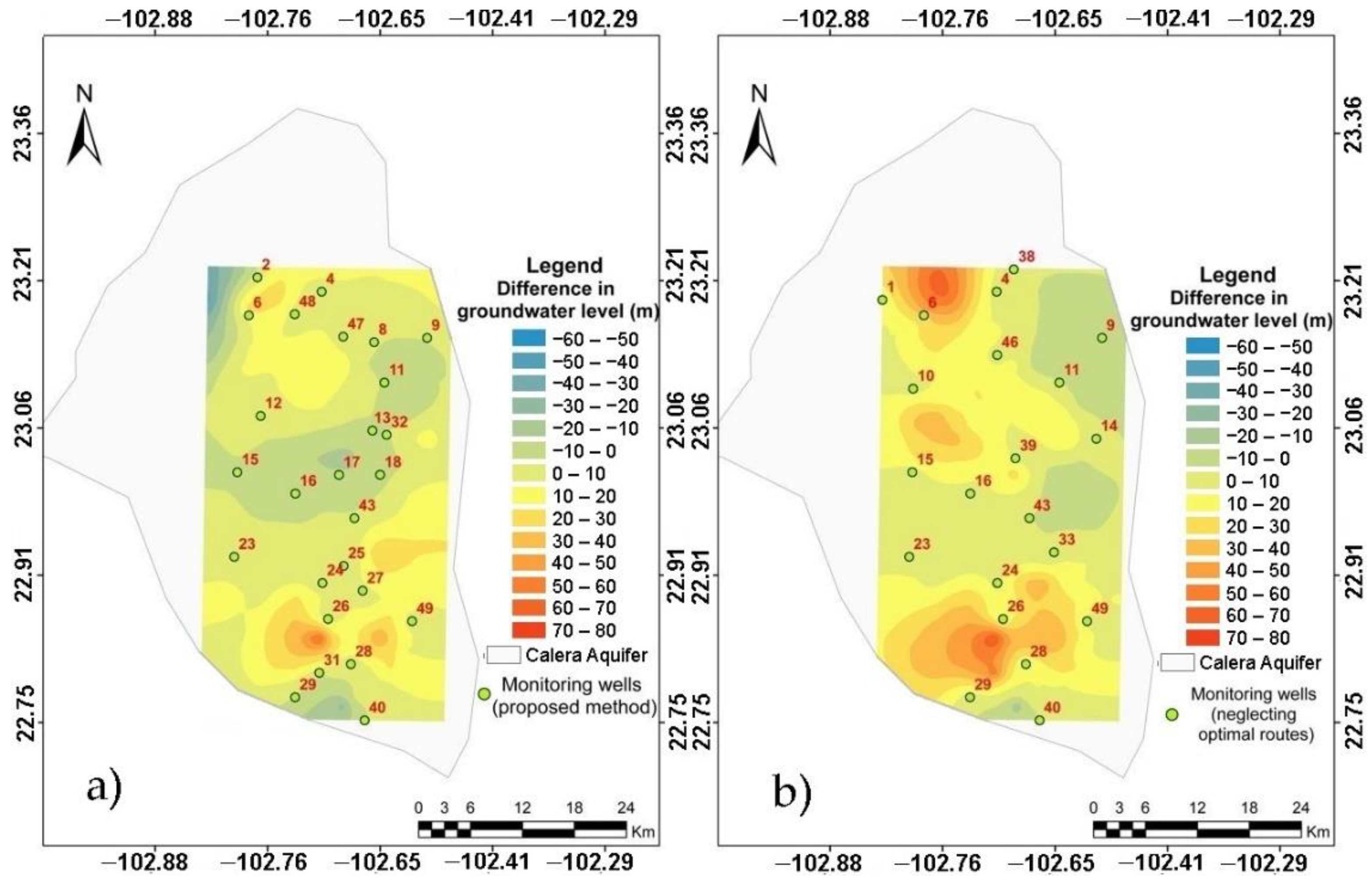
| Statistics | Complete Monitoring Network (49 Wells) | Selected Monitoring Network with the Proposed Method (26 Wells) | Selected Monitoring Network with the Júnez-Ferreira Method (21 Wells) |
|---|---|---|---|
| Average standard error (m) | 35.01 | 38.36 | 38.35 |
| Mean difference (m) | ------- | 5.76 | 12.46 |
| Mean Square difference (m2) | ------ | 179.76 | 394.68 |
| Root of the Mean Square Difference (m) | ------ | 13.41 | 19.87 |
| Maximum difference (m) | ------ | 74.92 | 86.63 |
| Minimum difference (m) | ------ | −57.38 | −19.83 |
Publisher’s Note: MDPI stays neutral with regard to jurisdictional claims in published maps and institutional affiliations. |
© 2022 by the authors. Licensee MDPI, Basel, Switzerland. This article is an open access article distributed under the terms and conditions of the Creative Commons Attribution (CC BY) license (https://creativecommons.org/licenses/by/4.0/).
Share and Cite
Cázares Escareño, J.; Júnez-Ferreira, H.E.; González-Trinidad, J.; Bautista-Capetillo, C.; Robles Rovelo, C.O. Design of Groundwater Level Monitoring Networks for Maximum Data Acquisition at Minimum Travel Cost. Water 2022, 14, 1209. https://doi.org/10.3390/w14081209
Cázares Escareño J, Júnez-Ferreira HE, González-Trinidad J, Bautista-Capetillo C, Robles Rovelo CO. Design of Groundwater Level Monitoring Networks for Maximum Data Acquisition at Minimum Travel Cost. Water. 2022; 14(8):1209. https://doi.org/10.3390/w14081209
Chicago/Turabian StyleCázares Escareño, Juana, Hugo Enrique Júnez-Ferreira, Julián González-Trinidad, Carlos Bautista-Capetillo, and Cruz Octavio Robles Rovelo. 2022. "Design of Groundwater Level Monitoring Networks for Maximum Data Acquisition at Minimum Travel Cost" Water 14, no. 8: 1209. https://doi.org/10.3390/w14081209