Linking Micropollutants to Trait Syndromes across Freshwater Diatom, Macroinvertebrate, and Fish Assemblages

Abstract

The ecological quality of freshwater ecosystems is endangered by various micropollutants released into the environment by human activities. The cumulative effects of these micropollutants can affect the fitness of organisms and populations and the functional diversity of stream ecosystems. In this study, we investigated the relationships between the joint toxicity of micropollutants and trait syndromes. A trait syndrome corresponds to a combination of traits that could occur together in communities due to the trait selection driven by exposure to these micropollutants. Our objectives were to (i) identify trait syndromes specific to diatom, macroinvertebrate, and fish assemblages and their responses to exposure, taking into account four micropollutant types (mineral micropollutants, pesticides, PAHs, and other organic micropollutants) and nine modes of action (only for pesticides), (ii) explore how these syndromes vary within and among the three biological compartments, (iii) investigate the trait categories driving the responses of syndromes to micropollutant exposure, and (iv) identify specific taxa, so-called paragons, which are highly representative of these syndromes. To achieve these objectives, we analyzed a dataset including the biological and physico-chemical results of 2007 sampling events from a large-scale monitoring survey routinely performed in French wadeable streams. We have identified five (diatoms), eight (macroinvertebrates), and eight (fishes) trait syndromes, either positively or negatively related to an increasing toxicity gradient of different clusters of micropollutant types or modes of action. Our analyses identified several key trait categories and sets of paragons, exhibiting good potential for highlighting exposure by specific micropollutant types and modes of action. Overall, trait syndromes might represent a novel and integrative bioassessment tool, driven by the diversity of trait-based responses to increasing gradients of micropollutant toxic cocktails.

1. Introduction

Aquatic ecosystems have been increasingly impaired by the worldwide intensification of human activities [1,2,3,4]. In this rapidly changing environment, the persistence of local populations greatly depends on their ability to cope with the interactive effects of the different stressors by selecting species over multiple spatial and temporal scales [5,6]. With thousands of chemical compounds and millions of tons released every year into aquatic ecosystems [7,8], understanding and assessing the cumulative effects of micropollutants (e.g., pesticides, polycyclic aromatic hydrocarbon (PAH), organic and mineral micropollutants) on aquatic species represents a daunting challenge, and even more so when considering their joint effects [9]. Thus, routine ecotoxicological studies perform a countless number of bioassays on organisms, including—but not limited to—fish (e.g., Oncorhynchus mykiss), macroinvertebrates (e.g., Daphnia magna), and microalgae (e.g., Pseudokirchneriella subcapitata) to assess their sensitivity to micropollutants. With the recent rise of the conceptual adverse outcome pathways (AOPs; [10,11]) framework, modes of action of chemical compounds are increasingly being investigated to identify the relationship between a compound and its molecular target and the cascade of effects at higher biological scales [12]. However, important knowledge gaps remain regarding the potential causal relationships across high biological levels of organization (i.e., populations, communities; [13,14,15]). Moreover, such relationships have been mainly investigated under controlled conditions, but much more rarely for the assessment of the ecological quality of environments in natura [16,17].

Meanwhile, recent advances in environmental risk assessment studies have demonstrated that community-wide changes can be mechanistically related to a given stressor and can be determined with ecological diagnostic tools [18,19,20,21]. Several of these tools are based upon the foundational concept that combinations of morphological, physiological, and behavioral characteristics, as well as ecological preferences of species (i.e., species traits) in a given biological assemblage, can indicate how species interact with their environment and inform on various habitat characteristics, including anthropogenic pressures [22,23,24]. This conceptual framework is based on the assumption that, because habitat is a flexible templet for the selection of species traits [25,26], combinations of biological traits and ecological strategies in natural communities result from evolutionary trade-offs between costs and benefits in the processes of adapting populations and communities to spatial and temporal variability in their environment [25,27]. Habitat filtering [28] and competition [29] are two major processes driving trait selection in local species assemblages. The former combines various natural environmental filters acting at different nested spatial and temporal scales [30] to anthropogenic pressures that are able to modify natural environmental filtering and dispersal-based processes of community assembly. The latter can exacerbate the effects of habitat conditions on trait selection via its effect on the fitness of individual organisms. Both selective processes lead to combinations of traits (i.e., the so-called “trait syndromes” [31,32]) that could be (i) specific to a given pressure category, (ii) specific to a given biological compartment, and (iii) used in turn to inform on the major causes of community impairment.

However, the effects of pressures on trait selection in communities are often difficult to predict [33], and a broad generalization about how environmental constraints structure community attributes is difficult to achieve [34,35,36]. Observed trends in species traits indeed often do not correspond to the details of the habitat templet predictions [27,37]. A given habitat does not act as a uniform templet for all the traits of all the species due to the complex combination of (i) direct sublethal effects of pressures on organisms and (ii) indirect functional effects that variously percolate through food webs [4]. Phylogenetic history and/or adaptive constraints can also lead to unexpected trade-offs of traits in this habitat [35,38,39]. An especially effective adaptation might indeed ensure the success of an organism in a given habitat without the need to achieve further traits. Different trait combinations can have the same adaptive advantage and then occur together in species assemblages with various proportions. Similar selective pressures can also result in different traits in different taxonomic lineages because adaptations are not equally achievable by distantly related organisms [30]. In addition, trait-based responses to natural and anthropogenic pressure gradients can differ among biological compartments. For example, in streams, benthic diatoms, macroinvertebrates, and fishes respond diversely to micropollutant exposure, hydrological regime alteration, or the hydromorphological degradation of reaches [21,40,41]. Moreover, benthic diatoms and macroinvertebrates, exhibiting lower dispersal capacities and shorter life cycles than fishes, should react more rapidly to lower levels of water quality degradation (i.e., be better early warning indicators of degradation [41]). In contrast, fishes, with higher migratory capacities and longer generation times might respond earlier to habitat restoration (i.e., be better late warning indicators [42]). This variety of response patterns justifies working on “trait syndromes” and adopting a “multi-biological compartment” approach (e.g., focusing simultaneously on diatoms, macroinvertebrates, and fishes) to optimally diagnose stream impairment.

In this study, we, therefore, surmised that integrating information on the toxicity, exposure, and modes of action (MoAs) of multiple micropollutants along with the trait syndromes of three major biological compartments in lotic ecosystems (diatoms, macroinvertebrates, and fishes) would improve the overall environmental risk assessment of micropollutants. We thus asked the four following questions:

(i) Are there particular trait syndromes associated with broad categories of micropollutants (e.g., mineral, organic, PAH) or to main pesticide MoAs (e.g., pesticides that target the biosynthesis of amino acids and proteins, cell membrane integrity, or lipid metabolism)?

(ii) Do diatom, macroinvertebrate, and fish assemblages differ in their trait-based responses to micropollutant types or modes of action?

(iii) Are specific traits mainly driving the responses of trait syndromes according to the modes of action of micropollutants?

(iv) Are there particular diatom, macroinvertebrate, and fish taxa that could be considered paragons of trait syndromes (i.e., efficient representatives of trait syndromes and indirectly of effects of micropollutants or pesticide MoAs), and potentially used as sentinel taxa in the survey of micropollutant exposure?

2. Material and Methods

2.1. Benthic Diatom, Macroinvertebrate, and Fish Data

To investigate the link between micropollutants and trait syndromes, we used data extracted from a national database (http://www.naiades.eaufrance.fr, accessed on 1 June 2020) maintained as part of the monitoring programs implemented in France following the European Water Framework Directive (WFD; [43]). This database gathers the abundances of three biological compartments, namely benthic diatoms, benthic macroinvertebrates, and fishes. The three biological compartments were sampled following standardized protocols, namely the normalized Biological Diatom Index sampling protocol [44], the multi-habitat sampling protocol for macroinvertebrates [45], and the standardized electrofishing protocol [46]. Here, we only kept the sampling events (i.e., “site x year” couples), during which the three biological compartments were sampled within a period of three months. Our work dataset was thus composed of three tables compiling the abundances of diatoms (1279 taxa), macroinvertebrates (344 taxa), and fishes (63 taxa) for 2007 sampling events, which exhibited a complete description of the chemical (a maximum of one pressure type without information) and hydromorphological pressures (no missing information). For further details on the pressure descriptions, see [47]. These sampling events were performed at 947 sites over the period of 2005–2015 (with an average of 2.1 sampling events per site).

The three abundance datasets were combined with three trait datasets, describing various biological attributes and ecological preferences of the taxa identified in each of the three abundance datasets. Qualitative traits have been described by a suite of nominal categories; for example, “aerial, passive”, “aerial, active”, “aquatic, passive”, and “aquatic, active” for the trait “Dispersal” applied to macroinvertebrates. Quantitative traits have been expressed by ordinal categories describing a gradient; for example, a gradient of maximal potential size via the categories “<0.5 cm”, “≥0.5–1 cm”, “≥1–2 cm”, “≥2–4 cm”, and “>4 cm” for macroinvertebrates. Thirteen traits have been taken into account for diatoms (58 categories), 25 traits for macroinvertebrates (114 categories), and 46 traits for fishes (178 categories). Additional information on the traits and trait categories is provided in [23] for diatoms, [22,48,49] for macroinvertebrates, and [24] for fishes. Traits were coded using either (i) a fuzzy-coding approach (i.e., by assigning to a given taxon an affinity score ranging from “0” (=no affinity) to “5” (=high affinity) to each category of the trait [50]); (ii) a disjunctive approach (i.e., the category is used (=1) or not used (=0) by the taxon). Before further calculations, all the affinity scores of a given taxon for a given trait were expressed as relative frequencies by dividing each affinity score by the sum of the scores of the taxon over all the categories of this trait. The trait descriptions are available in the Supplementary Materials (Tables S1–S3, for diatom, macroinvertebrate, and fish traits, respectively).

For each sampling event and biological compartment, the mean relative frequency of each trait category in each assemblage (i.e., the community-weighted mean; CWM) was calculated using the corresponding abundance and trait datasets and the following formula:

$${CWM}_m=\frac{{{\displaystyle \sum }}_i\left(R{A}_{mi}\times log\left(A_i+1\right)\right)}{{{\displaystyle \sum }}_{i}log\left(A_i+1\right)}$$

(1)

where CWM_m is the community-weighted mean of the trait category m for a given sampling event, RA_mi is the relative affinity of taxon i for the trait category m, and A_i is the abundance of the taxon i in the sampling event.

2.2. Calculation of Micropollutant Toxicity in Water

Environmental data were associated with the 2007 sampling events feeding the abundance datasets. If information on 174 micropollutants was available in our raw dataset, only 120 compounds or compound families were kept for the calculation of the joint toxicity of mixtures in the water of each sampling event (Table S4). Only the micropollutants with available (i) water concentration in the sampled sites (measured during routine stream monitoring in France; http://www.naiades.eaufrance.fr, accessed on 1 March 2021), (ii) toxicity value (expressed as the median effective concentration, EC₅₀) for the model species of the three biological compartments, and (iii) known mode of action (for pesticides) were selected for the calculation of their joint toxicity in water. These micropollutants belonged to five types—“mineral micropollutants”, “pesticides”, “polycyclic aromatic hydrocarbons (PAHs)”, “polychlorinated biphenyls (PCBs)”, and “(other) organic micropollutants”. The toxicity values were retrieved from three open databases—the Pesticide Properties DataBase (PPDB; http://sitem.herts.ac.uk/aeru/ppdb/, accessed on 1 March 2021), Malaj et al. (2014, [51]), and the INERIS database (https://substances.ineris.fr/fr/search, accessed on 1 March 2021). The modes of action were also retrieved for the 120 micropollutants using the R4P database [52]. Each pesticide has been allocated to a single mode of action among thirteen different MoAs (

Table 1. Main functions targeted by pesticides when referring to the R4P database. When the mode of action has not been identified (i.e., for the other micropollutant types), only the name of the pollutant type is given. For each, the total number of compounds (or compound families) involved and their codes for downstream analyses are provided. In the right column, a star (*) indicates the types of functions (or micropollutants) that were not kept in the following analyses (see the end of Section 2.2 for more details about the selection step).

Main Target Function or System (or Name of Pollutants)	Number of Compounds Involved	Code
Pesticides
Biosynthesis of amino acids and proteins	5	BAAPR
Biosynthesis of nucleic acids and precursors	1	*
Biosynthesis of pigments	3	PIGMT
Cell division or cytoskeleton	3	CYTO
Cell membrane integrity	2	CMEM
Cell signaling	3	*
Hormonal regulation	4	*
Lipid metabolism	4	LIPID
Multi-sites, multi-targets	4	MULTI
Nervous system, sensory system or muscles	18	NSSSM
Photosynthesis	15	PHOTO
Plant defense stimulation	1	*
Sterol metabolism	6	STERO
Other micropollutants
(other) Organic micropollutants	47	ORGA
PAH	8	PAH
PCB	1	*
Mineral micropollutants	5	MINER

). It was indeed not possible to allocate a precise mode of action for the four remaining micropollutant types. As a result, the MoA label provided in Table 1 corresponds to the function targeted by the compound according to the R4P database for pesticides, or simply the name of the micropollutant type for the other types. Afterwards, and for readability, all the MoAs (for pesticides) and the five other types of micropollutants have all been labeled as MoAs.

From this dataset compiling environmental concentrations and $E{C}_{50}$ values for each micropollutant, the toxicity of each MoA was expressed for each sampling event and each biological compartment as a “sum of toxic units” with the following formula:

$${TU}_{\mathrm{MoA}}={\displaystyle \sum }_i{\left[MP\right]}_i/E{C}_{50i}$$

(2)

where $T{U}_{\mathrm{MoA}}$ is the sum of the toxic units of all the micropollutants exhibiting the same MoA, ${\left[MP\right]}_i$ is the water column concentration of a micropollutant i exhibiting this MoA for a given sampling event, and EC_50i is the 50% effective concentration of the micropollutant i for a given biological compartment (diatoms, macroinvertebrates, or fishes). The water concentration of each micropollutant was calculated as the average of the available measurements over the year preceding the sampling date for a given biological compartment. All the values of EC₅₀ used in this study and their sources are available in the Supplementary Materials (Table S4). A toxic unit of “1” for a given biological compartment and a given micropollutant type means that the environmental concentration is equal to the EC₅₀. In other words, it is susceptible to inducing strong and acute toxicity. When it was not possible to calculate a sum of toxic units for a given sampling event and a given MoA due to the absence of information on micropollutant concentrations, we arbitrarily fixed the sum of toxic units as equal to zero. Given that the sums of toxic units were always lower than 1 across all the sampling events and biological compartments for four MoAs and PCBs, we have chosen to exclude these MoAs and PCBs from the following analyses (i.e., those identified by a star in Table 1). For the 12 remaining MoAs (9) and micropollutant types (3), the missing sums of toxic units, fixed to zero, were found in an average of 0.5 ± 0.7 MoA per sampling event.

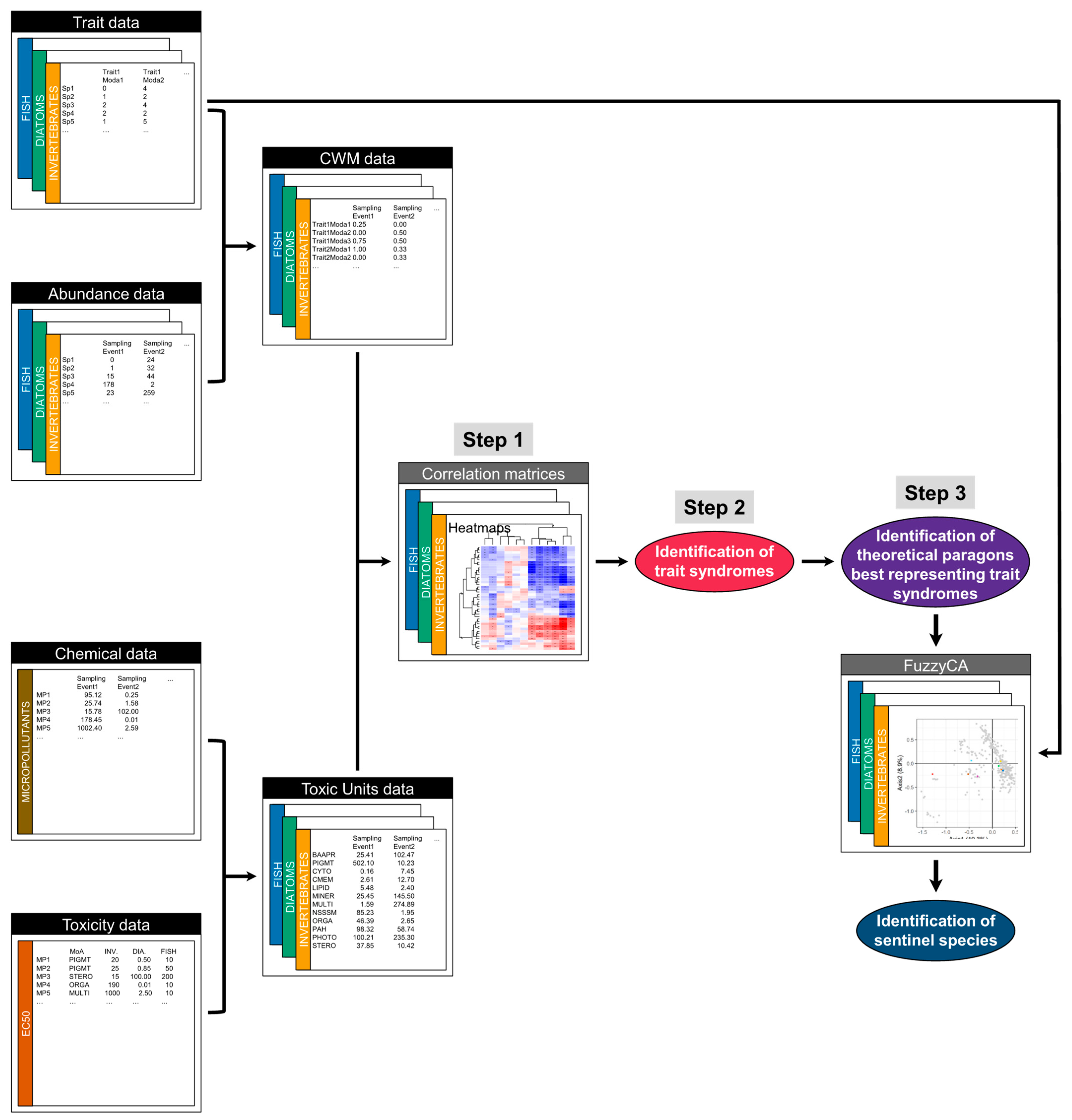
2.3. Statistical Analyses

In order to identify trait syndromes responding in a similar way to specific MoAs or groups of MoAs, we calculated the non-parametric correlation coefficients (Spearman’s rho; [53]) between each pair of trait category (from the CWM_m calculation) × MoA (expressed as the sum of toxic units). The calculations were done independently for each biological compartment from the database of the 2007 sampling events (Figure 1, step 1). The sums of the toxic units (x) were log(x + 1)-transformed before calculations. The strength and direction of the relationships between the trait categories and MoAs are illustrated by a heatmap drawn for each biological compartment. Only trait categories that correlated with at least three of the twelve MoAs selected for the analyses (Spearman’s test; p < 0.05 after Bonferroni’s correction) were selected for the heatmaps. This threshold of three significant correlations was chosen in order to limit the size of the heatmaps while still keeping its basic structure intact (i.e., the highlighted syndromes and groups of MoAs). The trait categories (rows) and the MoAs (columns) of the heatmaps were sorted using a hierarchical cluster analysis based on (i) a matrix of Euclidean distances directly calculated by the trait category/MoA correlations and (ii) Ward’s sum-of-squares linkage algorithm [54] to cluster either the trait categories or MoAs. According to the shapes of the corresponding dendrograms, we have defined the trait syndromes (i.e., clusters of trait categories) after the selection of a given partitioning level (i.e., a given Euclidean distance; Figure 1, step 2). We applied the commonly used “Phenon line” method [55], which requires the drawing of a line across the dendrogram at a certain similarity level. The selection of the partitioning level depends mainly on the specific shape of the dendrogram. We have marginally adapted this partitioning level to maximize the evenness of the trait categories among the trait syndromes and avoid having some trait syndromes with a too low or high number of trait categories.

If trait syndromes are key factors in explaining the relationships among communities and MoAs, individual trait categories within trait syndromes may differentially contribute to these relationships. To test this assumption, we analyzed the ability of individual trait categories to predict the toxic effect of micropollutants (considering their MoAs) compared to the trait syndrome. Therefore, the log(x + 1)-transformed sum of the toxic units of each MoA was modeled as a function of an individual trait category (expressed as CWM) significantly correlated with the considered MoA by using generalized additive models (GAM; [56]). Then, for a given MoA, the former models were compared (by using the generalized likelihood ratio test) to a global model, in which the values of log(x + 1)-transformed sums of the toxic units of this MoA were modeled as a function of all the trait categories of the corresponding trait syndrome. We used the results of these generalized likelihood ratio tests to identify the key trait categories for which models would not exhibit significant differences from the global model for a given MoA.

Last, we identified the model taxa, which could be considered as the best theoretical representatives (=the best paragons) of the trait syndromes within each biological compartment (Figure 1, step 3). For each trait syndrome identified by cluster analysis, we defined the trait profile of a theoretical taxon by assigning a value of “1” to all the trait categories involved in the trait syndrome and “0” to all the other trait categories. When several categories of the same trait were involved in the composition of a given trait syndrome, different paragons were defined corresponding to different combinations of scores for the categories of this trait. When a trait coded disjunctively had two categories involved in a given syndrome, two paragons were defined. The first one was coded “1” and “0” and the second one “0” and “1” for the first and second trait categories, respectively. When a trait was fuzzy-coded, we considered several combinations of the scores for the trait categories belonging to the syndrome so that the sum of each combination remained equal to 1. If two trait categories were involved in a given trait syndrome, the selected combinations of the scores were 0–1, 1–0, and 0.5–0.5 for the pairs of trait categories. If three trait categories were involved in the syndrome, the selected combinations of scores were 1–0–0, 0–1–0, 0–0–1, 0.66–0.33–0, 0.66–0–0.33, 0.33–0.66–0, 0.33–0–0.66, 0–0.66–0.33, 0–0.33–0.66, and 0.33–0.33–0.33 for the triplets of trait categories. No more than three categories of a given trait belonged to a given trait syndrome over the three biological compartments. All the paragons were projected as supplementary individuals on the factorial space defined by the first three axes of the fuzzy correspondence analysis (FCA) applied to the trait dataset. When several paragons were defined for a given trait syndrome, the location of an “average paragon” was also calculated as the centroid of the group of paragons based on their respective coordinates on the FCA factorial space, considering a number of successive FCA axes sufficient for taking into account at least 50% of the total variance in the dataset of the corresponding biological compartment. Finally, we identified the taxa (among diatoms, macroinvertebrates, and fishes, respectively) best representing each trait syndrome, by selecting the taxa that were closest to the location of the average paragon of each trait syndrome in the FCA factorial space, based on the Euclidean distance. To be representative of the trait syndromes, the selection of taxa was made using two successive criteria—(i) exhibiting the lowest distance to the average paragon of this trait syndrome (across all the trait syndromes), and (ii) being among the ten taxa with the shortest distance to this average paragon.

All statistical analyses were done using R software version 4.0.3 [57]. The correlation coefficients (Spearman’s rho) between each pair of trait category × MoA were calculated by using the cor.test() function. The heatmaps were drawn using the function heatmap2() from the package gplots [58]. The hierarchical cluster analyses allowed us to identify which trait syndromes were performed by using the hclust() function, with ward.D2 as the algorithm. Generalized additive models were done with the gam() function, and the models were compared using the anova.gam() function (package mgcv; [59]). Finally, the FCA was performed using the dudi.fca() function of the package ade4 [60], and the Euclidean distance among the FCA scores of each pair of “mean paragon × taxon” was estimated by using the dist() function.

3. Results

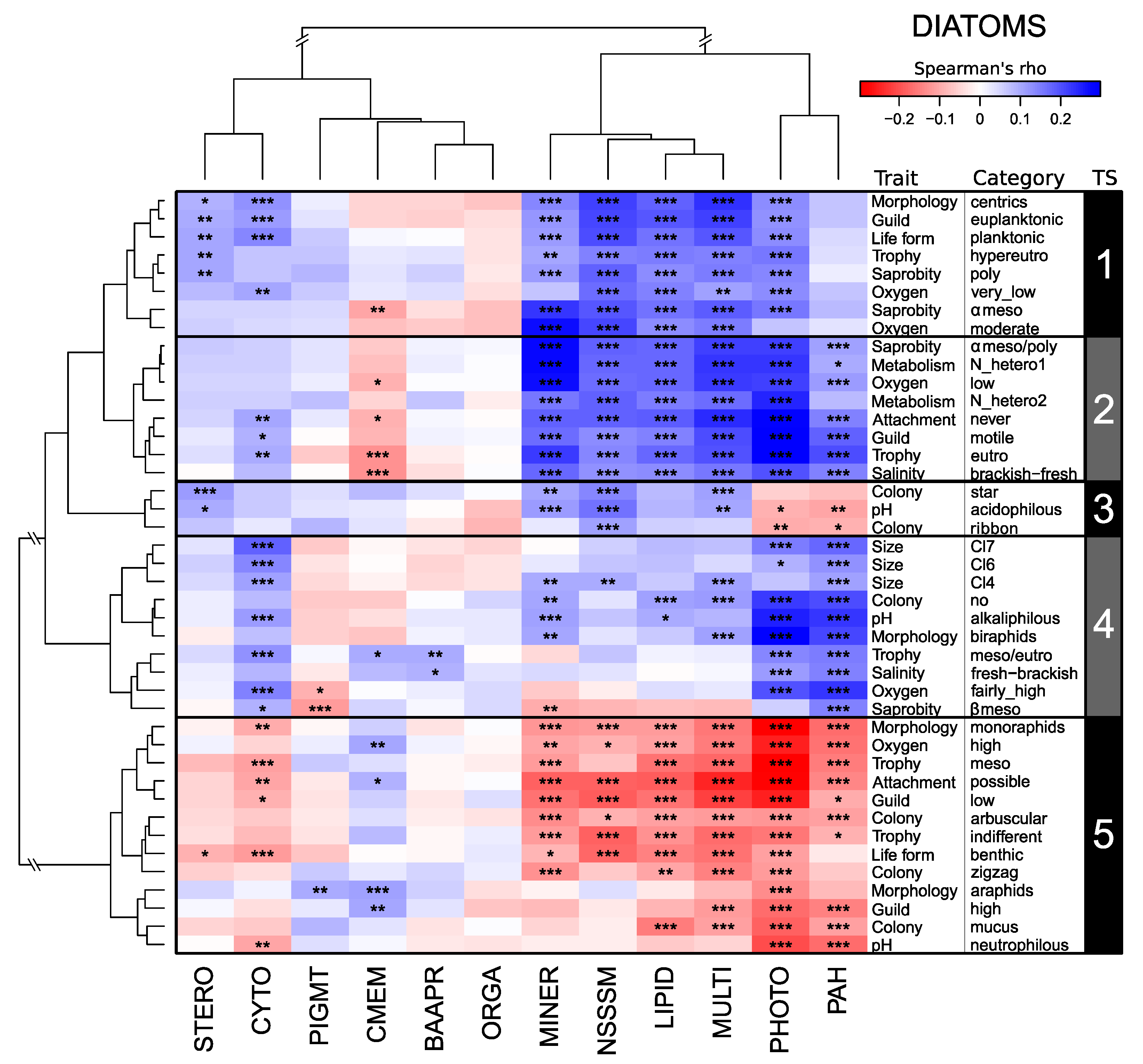
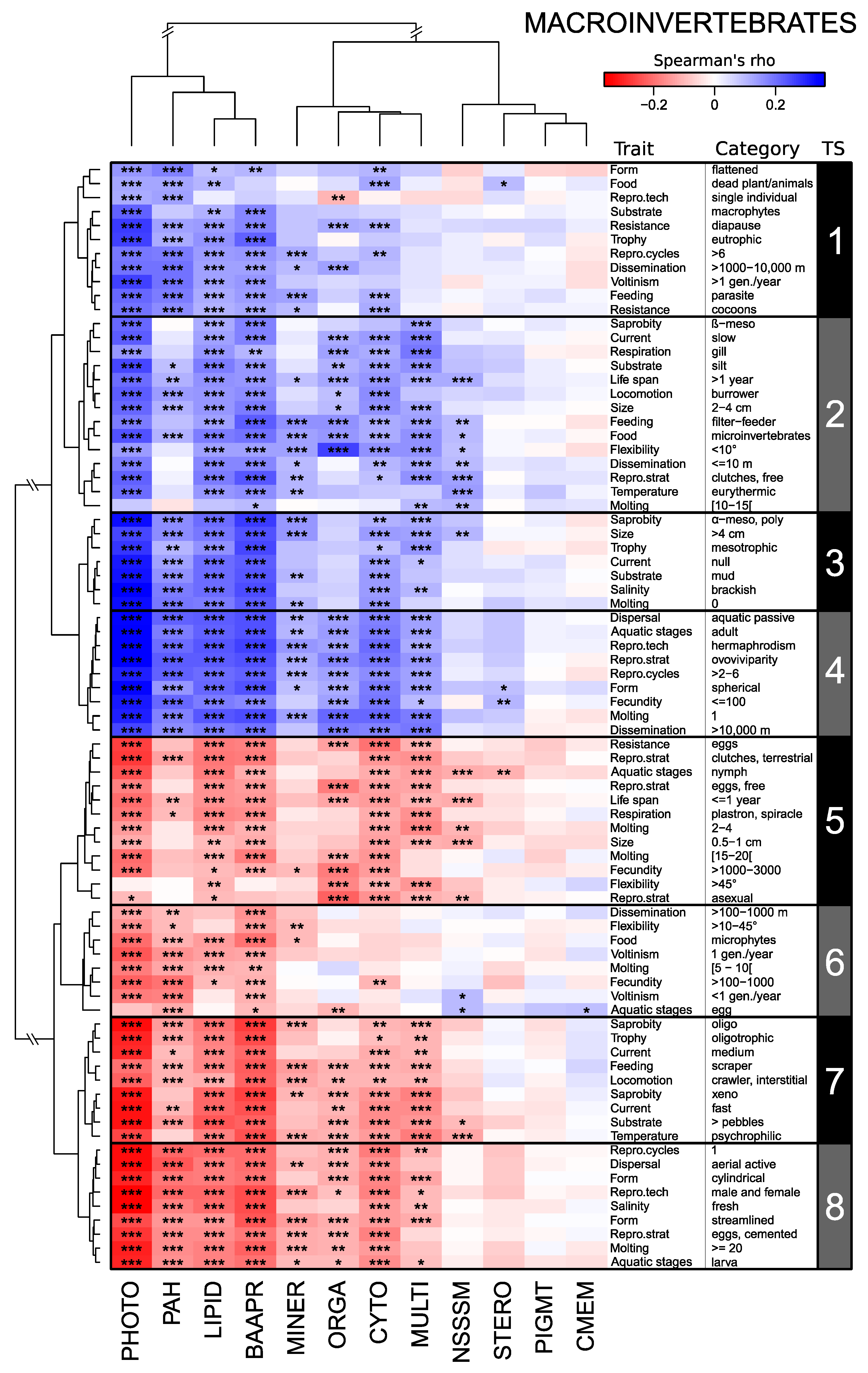
3.1. Links between Trait Syndromes and Modes of Action of Micropollutants

The clustering analysis based on correlations between exposure level (i.e., sums of toxic units) and trait category utilization by diatom assemblages identified two main clusters of MoAs and five trait syndromes (Figure 2). The first group was composed of six MoAs (MINER, NSSSM, LIPID, MULTI, PHOTO, and PAH) highly correlated with a large number of trait categories, whereas the second group gathered six MoAs (STERO, CYTO, PIGMT, CMEM, BAAPR, and ORGA) more weakly correlated to a smaller number of categories involved in trait syndromes. The MoAs of the first group showed quite similar correlation patterns, illustrated by mainly high positive correlations with the trait categories of TS1 to TS4 (except PHOTO and PAH with TS3) and high negative correlations with the trait categories of TS5. No significant relationships were observed between PAH and all the trait categories of TS1. Two contrasting correlation patterns were highlighted in the second group of MoAs. STERO and CYTO exhibited correlation patterns similar to those observed in the first group of MoAs with, in particular, positive correlations between CYTO and many trait categories of TS4. In contrast, PIGMT, CMEM, BAAPR, and ORGA had a rather idiosyncratic response pattern. For example, PIGMT exhibited an original pattern negatively correlated to all the trait categories of TS4.

At the trait category level, TS1 and TS2 gathered trait categories related to organic matter (“α-meso-” and “polysaprobic”, “very low”, and “moderate” oxygen requirements in TS1; “α-meso-polysaprobic” and “low oxygen” in TS2) and nutrient contamination tolerance (“hypereutrophy” in TS1; “eutrophy” in TS2). These two trait syndromes were distinguished by the presence in the second (TS2) of a trait category related to moderate salinity (“brackish–fresh” water). TS3 only included two colonial life forms (stars and ribbons) and one category related to low pH tolerance (acidophilous). TS4 gathered trait categories linked to life form (solitary, biraphids), size (the biggest size classes), and moderate tolerance to trophy (meso-eutrophy) and saprobity (β-mesosaprobity), albeit one category indicating taxa living in environments with fairly high oxygen levels. TS5 included trait categories exhibited by taxa sensitive to micropollutant exposure (i.e., mainly negatively correlated to increasing exposure), with trait categories related to diatom morphology and life forms (benthic, monoraphids/araphids, forming zigzag, mucous and arbuscular colonies, low and high guilds), but also to habitats characterized by high oxygen levels and mesotrophic conditions.

The clustering analysis based on the correlations between the exposure level and trait category utilization by macroinvertebrate assemblages identified three main clusters of MoAs and eight trait syndromes (Figure 3). PHOTO, PAH, LIPID, and BAAPR, included in the first group, were significantly correlated to all the trait syndromes, either positively (with TS1 to TS4) or negatively (with TS5 to TS8). PAH exhibited a specific pattern of correlations, with low levels of correlation to TS2 and TS5. The second group of MoAs (MINER, ORGA, CYTO, and MULTI) showed correlation patterns similar to those of the first group but with a lower proportion (or absence for MULTI) of strong, significant correlations with trait syndromes, in particular TS1 and TS6. ORGA was not correlated significantly to trait categories of TS3, and MINER only weakly correlated to TS5 (only one significant, negative correlation). In the third group of MoAs, STERO, PIGMT, and CMEM showed very few significant correlations with the trait categories of all the trait syndromes, whereas NSSSM displayed a higher number of significant correlations with the trait categories of TS2 (positive) and TS5 (negative).

The trait syndromes included mainly trait categories related to ecological preferences (e.g., >70% of trait categories in TS3 and TS7). The involved trait categories described affinities for high organic (α-meso- and polysaprobity) or moderate nutrient content (mesotrophy), depositional habitats (no current, mud), and brackish waters in TS3. In contrast, the trait categories in TS7 were related to low organic (xeno- and oligosaprobity) and nutrient content (oligotrophy), cold (psychrophilic), and coarse (flags/boulders/cobbles/pebbles), rheophilic habitats (medium to fast current velocity). Conversely, TS5 was only composed of biological trait categories linked to life history (presence of a nymphal instar, short life span, high number of molting events) and to reproduction (via eggs laid in terrestrial habitats or free in the water column, high fecundity, eggs as resistance forms). Two trait categories of TS5 (high body flexibility and asexual reproduction) slightly diverged from the first ones, with poorer correlation levels with PHOTO, PAH, and BAAPR. TS1 distinguished taxa with a flattened body, high voltinism, potential parthenogenesis, high number of reproductive cycles per individual, detritus as food, tolerance to high nutrient content (eutrophic), and preferences for macrophytic substrates. TS4 corresponded to taxa with a spherical form, hermaphroditic and/or ovoviviparous reproduction, moderate number of reproductive cycles per individual with a rather passive dispersion, and strong dispersal potential. TS8 gathered monovoltine species with a cylindrical or streamlined body, sexual reproduction, isolated and cemented eggs, active aerial dispersal, and preferences for freshwater habitats. TS2 included eurythermic and limnophilic filter-feeders with low body flexibility, poor dispersal potential, and preferences for β-mesosaprobic waters. In contrast, TS6 corresponded to monovoltine and semivoltine species with high body flexibility, aquatic eggs, biofilm feeding, and moderate dispersal potential and fecundity.

The clustering analysis based on the correlations between the sums of toxic units and trait category utilization by fish assemblages has provided two main groups of MoAs and eight trait syndromes (Figure 4). The first group, composed of BAAPR, MULTI, PHOTO, and LIPID, was positively correlated to most trait categories of TS1 to TS5 (except BAAPR, with five trait categories of TS1 and three trait categories of TS2) and negatively correlated with the trait categories of TS6 to TS8 (except BAAPR, with few trait categories of TS6). The second group of eight MoAs exhibited two contrasting correlation patterns. PAH, STERO, and CYTO had correlation patterns rather similar to those observed in the first group of MoAs, exhibiting either significant positive correlations with the trait categories of TS1, TS2 (except PAH), and TS5 and significant negative correlations with the trait categories of TS6 and TS8, but in far smaller numbers. MINER was the only MoA of this group correlated with several trait categories of TS2, TS3, TS5, TS7, and TS8. CMEM exhibited an original pattern, with negative (sometimes significant) correlations with trait categories of TS1 related to a long reproductive period duration (≥5 months), moderate tolerance to oxygen depletion, and preference for pelagic habitats.

TS1, TS3, TS7, and TS8 gathered mainly trait categories related to reproduction. Spawning starting in winter and ending in spring within a short period of phytophilic reproduction (2 months), medium egg diameter (1.5–2 mm), parental care, and tolerance to high temperatures were the trait categories of TS1. TS3 consisted of trait categories such as a spring spawning period, multiple spawning events (>6 cycles), moderate length of reproductive period (3 months), small egg diameter (<1.1 mm), high fecundity (>350,000 oocytes per spawning event), and short incubation period (≤7 days). TS7 included a long incubation period (>14 days), single spawning event, nest building, and low fecundity (<200 oocytes per spawning event). Finally, TS8 gathered trait categories such as spawning in the mineral habitats of running waters and spawning starting and ending in fall during a rather long reproductive period (4 months). These four trait syndromes may be also distinguished based on other traits. For example, TS7 and TS8 included trait categories related to dispersal—low ability to move against the current (TS7), minimum water height needed to swim and jump higher than 15 cm, and moderate distance traveled with the current (TS8). TS3 included a series of morphological trait categories related to larval length (4.2–6.3 cm), relative eye size (intermediate eye/head size ratio), caudal propulsion efficiency (low caudal peduncle throttling), relative maxillary length (low), and oral gap position (high oral gap position/body depth ratio). TS2 and TS4 gathered mainly trait categories related to morphology and feeding habits, for example, small and lateral eyes, low body mass (<22 g), and preferences for fine detritus and biofilm (TS2), or large body size (22.8–91.2 cm) and food preferences for coarse organic detritus, plants, or fish (TS4). TS2 also included trait categories linked to migration (catadromous/anadromous), whereas TS4 gathered trait categories describing tolerance to low oxygen levels and preference for lentic habitats. TS5 and TS6 gathered mainly trait categories linked to morphology and growth; for example, intermediate body mass (202–5100 g), high caudal propulsion efficiency, intermediate growth rate (TS5), or fusiform or streamlined body, high body mass (>5100 g), large size (>91.2 cm), high growth rate (>0.48–0.96 time⁻¹), and several ranges of organ/body ratios (TS6). TS5 also included moderate to high fecundity (45,000–350,000 oocytes), and stagnant water spawning (limnopar) on submerged plants, logs, gravel, and rocks (phyto.litho). TS6 also gathered several swimming attributes—a subcarangiform swimming mode, a high maximum swimming speed (>4–7 m·s⁻¹), and moderate obstacle crossing capacity (<3 m).

3.2. Trait Syndromes vs. Trait Categories in Explaining the Community–MoA Relationships

The comparison of individual and global models (with the generalized likelihood ratio test) revealed three patterns of relationships between the trait syndromes or trait categories and micropollutant MoAs (Table S5; also see Tables S6–S8). First, some trait syndromes always performed better than their individual trait categories for predicting the toxicity of MoAs. For example, TS1 has significantly greater predictive power for LIPID effects than individual trait categories, regardless of the biological compartment. Second, some individual models were not significantly different from their global models, suggesting that the corresponding individual trait categories have predictive power for the toxicity of MoAs similar to their trait syndrome. This pattern was actually observed in two contrasting situations, either when a given TS was poorly or highly correlated to a MoA. In the first case, for example, three out of eight trait categories in diatom assemblages (i.e., “Morphology_centrics”, “Life form_planktonic”, and “Trophy_hypereutro” in Table S5) were not significantly different from TS1 in predicting STERO but explained only a low proportion of variance (≤1.12%; Table S6). Similar results were observed for four out of eight categories (i.e., “Oxygen_low”, “Attachment_never”, “Trophy_eutro”, and “Salinity_brackish-fresh”) constituting TS2 of diatoms related to the prediction of CMEM effects. In the second case, for example, the proportions of macroinvertebrate species with one reproductive cycle per year (monovoltine; TS6) or tolerant to organic matter (α-meso- or polysaprobic; TS3) were highly correlated to LIPID, explaining a higher proportion of variance (3.94%–4.04%; Table S7). Similar response patterns occurred in diatoms and fishes (Table S2). For example, for fishes, a reproductive period length of four months was the main trait category of TS8 related to PHOTO, even though all the trait categories in this TS were highly correlated to this MoA (see Figure 4). Sometimes, the trait categories of a given syndrome highlighted by generalized likelihood ratio tests differed according to the MoA. For example, for macroinvertebrates, TS3 was well correlated to several MoAs, the different generalized likelihood ratio tests highlighting as key trait categories (i) α-meso- or polysaprobic taxa for LIPID, (ii) slow-flowing habitat preferences for BAAPR, and affinity for brackish waters for both PAH and CYTO (Table S5). Third, in some cases, the predictive power of MoA effects by one trait syndrome was not significantly different from those of the majority, or sometimes even all, of the constituent trait categories. For example, for macroinvertebrates, all the trait syndromes (except for TS2) had a lower predictive power of BAAPR effects than their constitutive trait categories (Table S5).

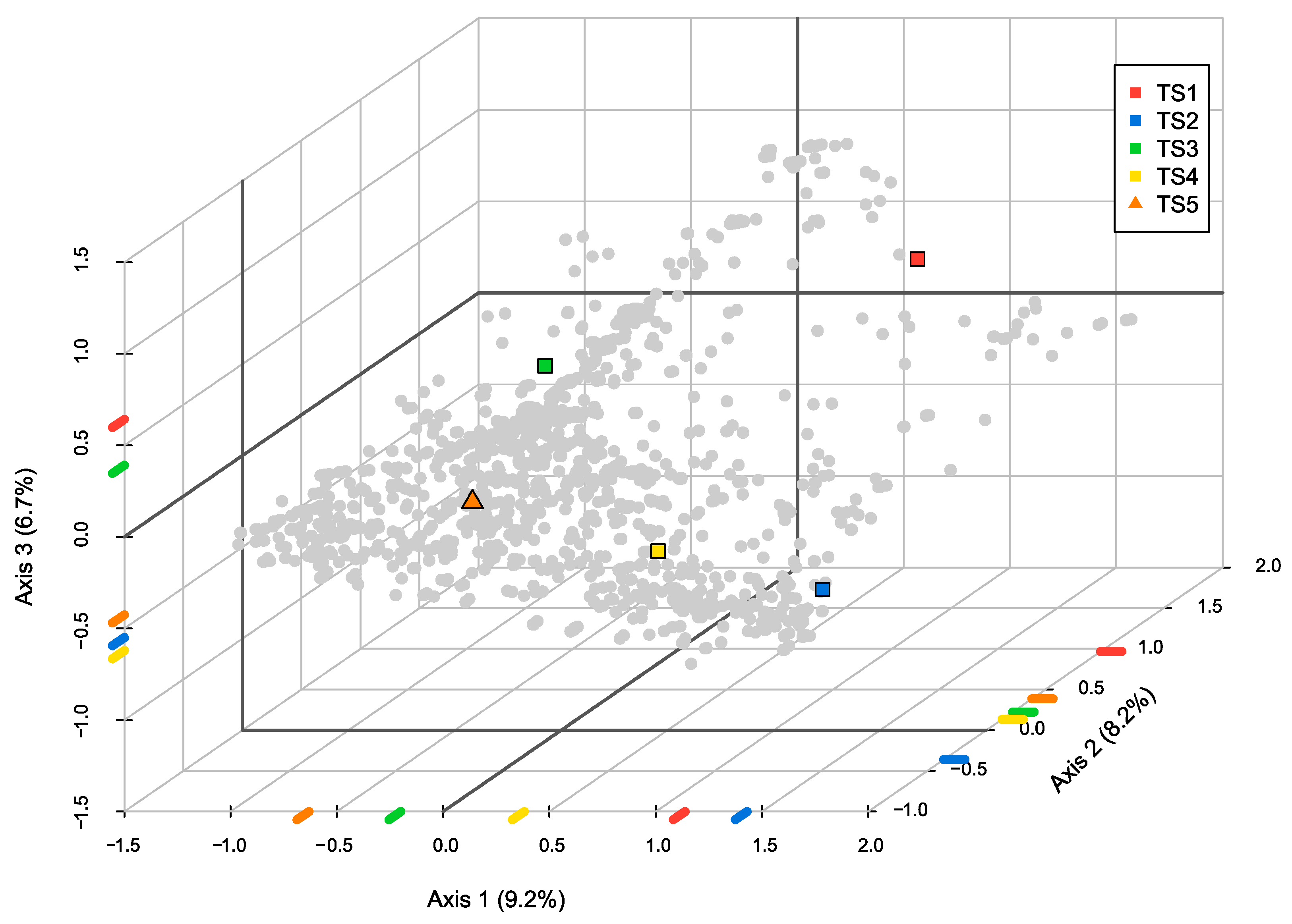
3.3. Paragons as Model Taxa Best Representing Trait Syndromes

Paragons were projected into a trait-based space explaining at least 50% of the total variance in the FCA, described by the first nine (diatoms), eight (macroinvertebrates), and eleven (fishes) axes defined by the FCA applied to each trait dataset. Then, using the Euclidean distance (ED) between each pair of “average paragon × taxon”, we identified taxa with trait combinations most similar to that of the paragon of a given trait syndrome. This procedure was repeated for the three biological compartments.

First, the average paragons of diatoms were widely dispersed in the FCA factorial space (Figure 5). TS1 and TS5 exhibited the paragons farthest from each other (ED = 4.59), in coherence with the results of the clustering analysis (Figure 2). The best representatives of TS5 were a homogeneous group of Achnanthidium (four species) and Achnanthes (six species) of the Achnanthaceae family (Table S9). In contrast, TS4 was best represented by species from five genera—Cavinula, Nitzschia (five species), Pinnularia, Stauroneis, and Surirella (two species) belonging to five families. TS1 was best represented by nine species of the Nitzschia genus and Stephanodiscus parvus. TS2 was typically represented by Navicula (five species), Luticola (four species), and Eolimna from two families. Finally, TS3 was best represented by eight species of the genus Eunotia (Eunotiaceae) and two species of the genus Grammatophora (Striatellaceae). Information at the species level is presented in Table S9.

Second, the average paragons of macroinvertebrate trait syndromes were gathered into two groups mainly along axis 1 (Figure 6). The first group was composed of the paragons of TS1 to TS4, gathering trait categories positively correlated to the sums of toxic units (Figure 3). The second group consisted of the average paragons of TS5 to TS8, including trait categories negatively correlated to the sums of toxic units. The Euclidean distances calculated between each pair of paragons attested a greater average inter-group distance (ED = 2.41) than the average intra-group distance (ED = 1.04). However, trait syndromes in the first group (TS1 to TS4) were more dispersed (ED = 1.39) in the factorial space than those of the second group (TS5 to TS8; ED = 0.68). The average paragons of TS5 and TS8 were closely located in the factorial space defined by the first three axes in the FCA even if these trait syndromes were rather distant in the clustering analysis, when considering the correlations among all trait categories (Figure 3). This spatial proximity in the FCA could be related to the common importance of mayflies—especially from the Baetidae and Leptophlebiidae families—in the ten best paragons of each trait syndrome (six genera in TS5 and eight genera in TS8) (Table S10). Another striking pattern was the remoteness of the location of TS4 along the first FCA axis. TS4 was exclusively represented by bivalves and crustaceans (both groups represented by five taxa). The best paragons of TS2 included a homogeneous group of nine Odonata genera (Aeshna, Anax, Calopteryx, Chalcolestes, Epitheca, Hemianax, Lestes, Platycnemis, and Sympecma) and one family (Coenagrionidae). TS6 and TS7 were best represented mostly by caddisflies (five and six genera or subfamilies, respectively). If the other best paragons of TS7 included stoneflies (Siphonoperla, Isoperla), beetles (Eubria), and dipterans (Blephariceridae); those of TS6 were more diverse taxonomically (Emmericia, Isonychia, Brachythemis, Capnia, and Stratiomyidae). The best paragons of TS1 included bivalves (Unio, Anodonta, and Potomida), leeches (Glossiphoniidae and Piscicolidae), and disparate taxa of crustaceans, bryozoans, planarians, and Nemathelminthes. Finally, TS3 was represented by gastropods (genera from six families), beetles (Spercheus and Hydrophilinae), oligochaetes, and Prostoma.

Third, the results of the FCA showed that the average paragons of fish trait syndromes were gathered into groups depending on the sign of the correlation between the sum of toxic units corresponding to a given MoA and trait category utilization by fish assemblages (Figure 7). The first group was composed of average paragons whose trait categories (from TS1 to TS5) were positively correlated with the gradient of exposure. The second group was composed of paragons whose trait categories (from TS6 to TS8) were negatively correlated with the gradient of exposure. Globally, the average inter-group distance (ED = 2.34) was greater than the average intra-group distance (ED = 1.00). However, TS1 to TS5 were more dispersed (ED = 1.07) than TS6 to TS8 (ED = 0.76). The average paragons of TS3, TS4, and TS5 were closely located along the first three factorial axes of the FCA (Figure 7). These paragons were represented exclusively (TS3) or mostly (TS4 and TS5) by Cyprinidae species (Table S11). The best representatives of TS2 were rather isolated at the positive side of the third FCA axis and mainly represented by two families of diadromous species (Petromyzontidae and Anguillidae). The average paragons of TS1 and TS7 had rather close positions along the first three FCA axes (Figure 7) despite belonging to clearly different clusters (Figure 4). They were mainly represented by species from four common families (Centrarchidae, Cyprinidae, Gobiidae, Percidae). Last, TS6 and TS8 were the only trait syndromes with paragons best represented by Salmonidae species.

4. Discussion

4.1. Trait Syndromes in Diatom, Macroinvertebrate, and Fish Assemblages

Due to the selected statistical approach, the trait syndromes identified for each biological compartment (between five and eight) were mainly composed of trait categories generally either all positively or all negatively related to the toxicity of the studied micropollutant types and MoAs. Coherently, trait syndromes displaying positive responses to increasing toxicity were mostly represented by trait categories usually observed in ubiquist species and/or r-strategists (e.g., eurytopes, generalists). In contrast, trait syndromes with negative responses to increasing toxicity gathered attributes of stenoecic, sensitive species and/or K-strategists (e.g., stenotopes, specialists). These responses were consistent with what has been observed in other studies in a similar geographical context (for diatoms: [23]; for macroinvertebrates: [22,47,61]; for fishes: [24]; also see [62] for the three biological compartments).

The trait syndromes of diatoms were mainly dominated by the trait categories linked to ecological preferences, for example, trophy, pH, or oxygen levels. Such an observation may easily be explained by the smaller number of biological traits in the diatom trait dataset compared to the macroinvertebrate and fish trait datasets, which included both a larger number of traits and many more numerous life-history and morphological traits. Trait syndromes positively related to high toxicity levels included mostly characteristics of diatoms found in nutrient and/or organic matter-contaminated media [63], with biological traits enabling the cells to cope with the lack of light or even to move in the biofilm matrix. In contrast, trait syndromes negatively related to high toxicity levels were rather characteristic of media less polluted, with various traits related to colonies, morphology, and guilds. The response patterns of diatom trait syndromes were also in line with previous studies regarding pesticide contamination. For example, the motile feature of diatoms was already taken as a parameter to identify a species “not at risk” in the diatom SPEAR index specific to herbicides [64]. The opposition in life form and morphology was also consistent with previous findings, with motile and biraphids species rather linked to a lower sensitivity to herbicides [65] and high profile species rather linked to less herbicide-contaminated sites [66]. Moreover, TS4 exhibiting strong positive correlations between the largest size classes and PAH exposure was in line with a previous observation stating that exposure to such compounds led to an increase in diatom cell biovolume [67].

Macroinvertebrate trait syndromes positively related to high toxicity levels frequently included adaptations allowing for pollution avoidance or tolerance (high dispersal ability, ovoviviparity, several forms of resistance), generally observed in non-insects living in slow-flowing waters. In contrast, trait syndromes negatively related to high toxicity levels were typical of pollution-sensitive taxa, more frequently found in some insect orders (preference for fast-flowing, oligotrophic habitats, high number of molting events, aquatic larval instars, and pupae). This typical opposition between insects and non-insects, usually observed between the upstream section of streams often less polluted and the downstream section often more severely impacted [68], was further confirmed by the identified paragons. The trait syndromes identified in this study did exhibit some similarities with those previously identified in North America [35]. For example, Poff et al. [35] identified two trait syndromes, one grouping rheophilic, flying, semivoltine taxa, and another one gathering eurythermic, polyvoltine, and filter-feeding taxa. Although both trait syndromes of Poff et al. [35] did not correspond exactly to those identified in this study, the corresponding trait categories at least occurred on the same major branch of the dendrogram in the macroinvertebrate-based heatmap (Figure 3).

Similarly, the trait syndromes of fishes highlighted an opposition between the traits found in the taxa of headwaters (sensitive to a low level of exposure to micropollutants and, therefore, negatively linked to an increasing sum of toxic units for MoAs) and traits typical of taxa from downstream sections of rivers. Trait syndromes negatively linked to high micropollutant exposure levels were indicative of long-lived K-strategists (high weight, large length, late maturity), intolerant to low oxygen levels, and living in fast-flowing water (albeit with a low dispersal potential). Trait syndromes positively linked to high micropollutant exposure levels were indicative of taxa found in slow-flowing waters, able to live in a large range of temperature, current velocity, and oxygen level, and feeding on detritus and plants, potentially r-strategists (e.g., exhibiting a high number of oocytes). The diversity of trait categories found in all the fish trait syndromes was quite high compared to that of diatoms and macroinvertebrates, but it was actually indicative of the high number and diversity of traits taken into account in the fish dataset. Winemiller et al. [69] did observe that due to a high number of traits linked to body shape in their dataset, such traits frequently drove trait-based species ordination. In our dataset, such traits were also quite frequent (32% of the trait categories), but it seems that they did not significantly drive the composition of fish trait syndromes. Only TS6 appeared to gather a lot of trait categories linked to body shape (8/19). Interestingly, TS2, which contains the trait category cata-/ana-dromous, was the only fish trait syndrome well correlated with NSSSM. In addition, potamodromous species and the absence of parental care were grouped in the same trait syndrome (TS6), similarly to the observation of Comte and Olden [70].

The trait syndromes we identified seemed to globally correspond to trait links observed in other studies (e.g., for diatoms: [63,67]; for macroinvertebrates: [35]; for fishes: [69,70]). The novelty of our approach lies in the fact that we used the link between the trait categories and the exposure/toxicity of MoAs to define the trait syndromes. We may even hypothesize that the observed similarities between our MoA-based trait syndromes and other trait syndromes already published would reinforce the hypothesis of micropollutant exposure as a driver of trait selection.

4.2. Relevance and Complementarity of Trait Syndromes for Bioassessment

Our analyses have shown that clusters of MoAs did change depending on the studied biological compartment. The trait syndromes were usually well related to half of the studied MoAs, whatever the biological compartment. Therefore, the majority of the trait syndromes seemed to be more linked to the global degradation state of the studied streams rather than to degradation linked to a specific MoA, probably due to the cocktail effect of exposure to micropollutants, when streams are multi-contaminated by micropollutants (especially pesticides) exhibiting various MoAs. Nevertheless, a small subset of trait syndromes did exhibit either (i) a limited number of significant relationships with MoAs, such as TS4 for diatoms or TS6 for macroinvertebrates (Figure 2 and Figure 3), or (ii) some opposite relationships with different MoAs, for example, positively related to the majority of the MoAs, but negatively related to a few others, such as TS2, TS3, and TS5 for diatoms (Figure 2). The latter type of trait syndromes was more frequently observed for diatoms.

Some MoAs were well correlated with the majority of the trait syndromes across all biological compartments. PHOTO and LIPID were indeed always grouped together, whatever the biological compartment. This common pattern may indicate a similar, indirect response of consumers to, for example, herbicides or fungicides, due to the direct effect of such pesticides on the nutritional quality/quantity of primary resources (biofilms, macrophytes) [71], or even to bioaccumulation at higher trophic levels [72].

CMEM and PIGMT were poorly correlated to all the trait syndromes, whatever the biological compartment. For CMEM, this absence of a significant relationship with trait syndromes may be explained by (i) a low number of molecules taken into account (n = 3; Table 1), and/or (ii) rather low toxicity levels of corresponding micropollutants for the three biological compartments, maybe due to a low number of significantly impacted sampling events (see Figure S1 in the Supplementary Materials). PIGMT also corresponded to a low number of molecules (n = 2; Table 1). However, their level of toxicity was quite high for diatoms (see Figure S1). Nevertheless, no trait syndrome was significantly linked with PIGMT, even for diatom assemblages. We may hypothesize that we did not investigate the relevant trait-based metrics for such MoAs. For example, PIGMT toxicity could be rather linked to metrics related to diatom pigment composition (e.g., carotenoids vs. chlorophyll). We may also hypothesize the potential antagonistic effects leading to the absence of a significant trait syndrome response.

Overall, our results have highlighted the complementarity of the studied biological compartments for potentially indicating similarities among multi-target MoAs. Moreover, streams may be at greater risk if mixtures of micropollutants exhibit synergistic effects, even if their concentrations are rather low or moderate [73,74]. The trait syndromes based on their patterns of responses to MoAs may therefore be pertinent to indicate exposure to mixtures of micropollutants with synergistic effects or with effects varying according to the biological compartment.

4.3. Key Trait Categories Driving Trait Syndrome Responses

We have tested the assumption that trait syndromes performed better than individual trait categories when predicting the level of exposure to micropollutants with various MoAs. Our analyses neither denied nor confirmed this assumption but have rather well highlighted three patterns of relationships.

The first pattern (i.e., trait syndrome-based GAM performance > all the individual trait category-based GAM performances) suggests that all the complementary information brought by individual trait categories is necessary to accurately evaluate the impairment level of micropollutant exposure in the environment. This first pattern was actually observed in the majority of the “trait syndrome × MoA” couples (i.e., 75%, 81%, and 91% of the pairs, respectively, for diatom, macroinvertebrate, and fish assemblages), underlining again the pertinence of trait syndromes to predict the biological effect of exposure to micropollutants.

The second pattern (i.e., performance of few specific trait category-based GAM = trait syndrome-based GAM performance) may arise when a given micropollutant (or a cocktail of micropollutants) has a strong impact on organisms and is selecting (for or against) specific trait categories. This pattern was sometimes observed for MoAs that were poorly correlated to most of the trait categories describing a given biological compartment over all the trait syndromes. For example, the link between the vertical position of fish eyes and cell membrane integrity alteration (CMEM) was positive with the trait category “Ratio.eye.vertical.posit_0.47–0.55” and negative with the trait category “Ratio.eye.vertical.posit_0.55–0.65”, which potentially provide information on the position of fish and/or its prey in the water column [75]. In this situation, the corresponding trait categories could be considered as categories of key traits to further study when trying to relate exposure to micropollutants with a given MoA (here, CMEM), even maybe as potential metrics for stream bioassessment. Moreover, we have sometimes observed that key trait categories of a given syndrome may change depending on the MoA (e.g., TS3 for macroinvertebrates). One plausible explanation would be simply that trait syndromes have been aggregated based on the correlations calculated over all the MoAs. A given trait syndrome could, therefore, gather trait categories exhibiting few contrasting links with some of the studied MoAs.

The third pattern (i.e., performance of many individual trait category-based GAM performances = trait syndrome-based GAM performance) was mainly observed for MoAs that were usually poorly correlated to most of the trait syndromes (e.g., CMEM and MULTI for diatoms, BAAPR for macroinvertebrates). This pattern may arise if high exposure levels to micropollutants with such MoAs were observed in a very limited number of sampling events or sites in the dataset. Nevertheless, this pattern may also contribute to the identification of key trait syndromes. For example, TS2 was a key trait syndrome for macroinvertebrates (see Tables S5 and S7), as it was the only one exhibiting a GAM always better than all the GAM based on each of the trait categories belonging to this syndrome (i.e., the first pattern), whereas all the other trait syndromes did not exhibit GAM better than their own trait categories (i.e., this third pattern).

Overall, all these results have highlighted the importance of including diverse and complementary biological and ecological information when evaluating the environmental risk induced by cocktails of pollutants.

4.4. Paragons as Model Taxa Best Representing Trait Syndromes

We furthered our analysis of trait syndromes with the identification of paragons, that is, taxa highly specific to the combination of trait categories highlighted by the syndromes. These paragons are of interest because they could be used as sentinel species, by (i) using their abundance, or even presence/absence, to develop new metrics or indices indicating the level of exposure of biotic assemblages to particular clusters of micropollutants/MoAs, as identified with the heatmaps, or by (ii) using them as new model species for ecotoxicological bioassays.

The best representatives of the five diatom trait syndromes have not been commonly used as model species in bioassays. The genus Nitzschia has been commonly used in laboratory studies, but mainly via the species N. palea (e.g., [76]), which is of interest but does not belong to the paragons. The same comment is also valid for other genera such as Achnanthidium or Eolimna (e.g., [77]). Our study has suggested new taxa that could be of interest for general micropollutant contamination, such as Nitzschia capitellata or Stephanodiscus parvus. The last one was recently highlighted as an indicator of stress induced by anthropogenic contamination in lakes [78]. In contrast, several species of the Achnanthes genus were identified as representatives of the trait syndrome strongly related to low levels of toxicity. That genus has been also identified as one of the main sensitive genera to different compounds such as pesticides and lead [79]. However, the cryptic diversity of benthic diatoms also has to be considered. Intra-species variation in sensitivity can indeed be non-marginal depending on the taxon [80] and could interfere with such signals based on in situ studies. One diatom trait syndrome (TS3) comprised only three trait categories, with two categories describing the form of the colony (either a ribbon or a star) and the third a preference for acidic waters. Moreover, this syndrome exhibited a positive link with MINER, NSSSM, and maybe STERO, and a negative link with PHOTO and PAH. The main paragon of TS3 was the genus Eunotia. This genus is known to tolerate acidic water [81]. The presence and/or abundance of this taxon could, therefore, be used to define a specific and pertinent bioindicator of the exposure level to a mixture of MoAs positively linked to TS3.

Macroinvertebrates identified as paragons of the trait syndromes positively linked with increasing exposure to MoAs frequently included taxa already and frequently used as model species in bioassays, for example, Lymnaea spp. in TS3 [82], and Gammaridae [83,84], Dreissena spp. ([85,86], and Corbicula spp. [87] in TS4. In contrast, the paragons of TS6 and TS7, both negatively linked with increasing MoAs exposure, included caddisflies and stoneflies. Both taxonomic groups have been frequently used as bioindicators of low anthropogenic pressures and good ecological quality [88], but rarely used as model species given the great difficulty in controlling the entire biological cycle of these species in laboratory conditions [89].

Similar to other biological compartments, paragons of fishes displayed either positive or negative correlations with exposure to micropollutants with various MoAs. For instance, Cyprinus carpio (representative of TS3), a common species found in European streams, was positively related to pesticide exposure with LIPID, BAAPR, and PHOTO MoAs. In contrast, Salmo trutta (representative of TS8) was negatively related to the same pesticide MoAs. Although the sensitivity of C. carpio and S. trutta to environmental chemical exposure is relatively well known [90,91], important ecotoxicological knowledge gaps remain for many other fish species identified as representative taxa using our approach (e.g., species of the Petromyzontidae family—Lampetra planeri, L. fluviatilis, Petromyzon marinus from TS2). In that sense, our approach could help identify these important knowledge gaps.

One limitation of our approach is that direct effects of micropollutants on representative taxa or sentinel species and indirect effects via biological interactions can hardly be disentangled. For instance, chemical stressors can indirectly impair sentinel species through their prey such as mayflies or stoneflies [92]. However, the identification of pertinent sentinel species highly specific to a given MoA could be further driven by the key trait categories we identified (see the previous section). For example, for MULTI, the best paragon of diatom assemblages could be a biraphid species (Table S5). Coupling the identification of key trait categories and sentinel species could, therefore, prove to be a powerful tool for improving the diagnosis of complex micropollutant exposures.

5. Conclusions and Perspectives

In summary, our study has demonstrated that large-scale empirical data allow for highlighting strong relationships among many micropollutant types or modes of action and diverse combinations of trait-based attributes (=trait syndromes) from freshwater benthic diatom, benthic macroinvertebrate, and fish communities. Trait syndromes exhibited both consistent and specific responses to combinations of main micropollutants and pesticides’ modes of action across the three biological compartments over a large-scale set of various environmental situations. Individual trait categories contributed to varying extents to those responses. Further evaluating which trait(s) contributed most to the observed responses will allow for inferring more precisely potential ecological mechanisms at play. Last, we have been able to summarize trait–micropollutant relationships into a handful of representative taxa that could be used as sentinel species when assessing in situ ecotoxicological risks.

Evaluating the response of thousands of aquatic organisms to thousands of chemical compounds, which can have synergistic or antagonistic effects when present in combination, is a daunting challenge. Our community-level approach using functional attributes of species offers a complementary method to those developed from cellular to individual levels (e.g., adverse outcome pathways, in vitro and in vivo toxicity extrapolations, high-throughput testing methods). For example, our approach can pinpoint specific combinations of micropollutants particularly widespread in streams and on which ecotoxicological studies could be focused. On a more applied side, sentinel species might be used by environmental managers to help in undertaking appropriate mitigation measures. Regarding the overwhelming number of long-time used and new micropollutants released every year into aquatic ecosystems, it is of utmost importance for ecosystem health to find approaches allowing for an acute understanding of multi-species biological responses to cocktails of chemical stressors.

References

1. Matthaei, C.D.; Piggott, J.J.; Townsend, C.R. Multiple stressors in agricultural streams: Interactions among sediment addition, nutrient enrichment and water abstraction. J. Appl. Ecol. 2010, 47, 639–649. [Google Scholar] [CrossRef]
2. Luo, K.; Hu, X.; He, Q.; Wu, Z.; Cheng, H.; Hu, Z.; Mazumder, A. Impacts of rapid urbanization on the water quality and macroinvertebrate communities of streams: A case study in Liangjiang New Area, China. Sci. Total Environ. 2018, 621, 1601–1614. [Google Scholar] [CrossRef]
3. Embke, H.S.; Rypel, A.L.; Carpenter, S.R.; Sass, G.G.; Ogle, D.; Cichosz, T.; Hennessy, J.; Essington, T.E.; Vander Zanden, M.J. Production dynamics reveal hidden overharvest of inland recreational fisheries. Proc. Natl. Acad. Sci. USA 2019, 116, 24676–24681. [Google Scholar] [CrossRef]
4. Haase, P.; Pilotto, F.; Li, F.; Sundermann, A.; Lorenz, A.W.; Tonkin, J.D.; Stoll, S. Moderate warming over the past 25 years has already reorganized stream invertebrate communities. Sci. Total Environ. 2019, 658, 1531–1538. [Google Scholar] [CrossRef] [PubMed]
5. Feld, C.K.; Hering, D. Community structure or function: Effects of environmental stress on benthic macroinvertebrates at different spatial scales. Freshw. Biol. 2007, 52, 1380–1399. [Google Scholar] [CrossRef]
6. Tóth, R.; Czeglédi, I.; Kern, B.; Erős, T. Land use effects in riverscapes: Diversity and environmental drivers of stream fish communities in protected, agricultural and urban landscapes. Ecol. Indic. 2019, 101, 742–748. [Google Scholar] [CrossRef] [Green Version]
7. Schwarzenbach, R.P.; Escher, B.I.; Fenner, K.; Hofstetter, T.B.; Johnson, C.A.; von Gunten, U.; Wehrli, B. The Challenge of Micropollutants in Aquatic Systems. Science 2006, 313, 1072–1077. [Google Scholar] [CrossRef]
8. Persson, L.; Carney Almroth, B.M.; Collins, C.D.; Cornell, S.; de Wit, C.A.; Diamond, M.L.; Fantke, P.; Hassellöv, M.; MacLeod, M.; Ryberg, M.W.; et al. Outside the Safe Operating Space of the Planetary Boundary for Novel Entities. Environ. Sci. Technol. 2022, 56, 1510–1521. [Google Scholar] [CrossRef]
9. Tang, J.Y.M.; McCarty, S.; Glenn, E.; Neale, P.A.; Warne, M.S.J.; Escher, B.I. Mixture effects of organic micropollutants present in water: Towards the development of effect-based water quality trigger values for baseline toxicity. Water Res. 2013, 47, 3300–3314. [Google Scholar] [CrossRef]
10. Ankley, G.T.; Bennett, R.S.; Erickson, R.J.; Hoff, D.J.; Hornung, M.W.; Johnson, R.D.; Mount, D.R.; Nichols, J.W.; Russom, C.L.; Schmieder, P.K.; et al. Adverse outcome pathways: A conceptual framework to support ecotoxicology research and risk assessment. Environ. Toxicol. Chem. 2010, 29, 730–741. [Google Scholar] [CrossRef]
11. Ankley, G.T.; Edwards, S.W. The adverse outcome pathway: A multifaceted framework supporting 21st century toxicology. Curr. Opin. Toxicol. 2018, 9, 1–7. [Google Scholar] [CrossRef] [PubMed]
12. Müller, M.E.; Vikstrom, S.; König, M.; Schlichting, R.; Zarfl, C.; Zwiener, C.; Escher, B.I. Mitochondrial Toxicity of Selected Micropollutants, Their Mixtures, and Surface Water Samples Measured by the Oxygen Consumption Rate in Cells. Environ. Toxicol. Chem. 2019, 38, 1000–1011. [Google Scholar] [CrossRef]
13. Schäfer, R.B.; Gerner, N.; Kefford, B.J.; Rasmussen, J.J.; Beketov, M.A.; de Zwart, D.; Liess, M.; von der Ohe, P.C. How to characterize chemical exposure to predict ecologic effects on aquatic communities? Environ. Sci. Technol. 2013, 47, 7996–8004. [Google Scholar] [CrossRef] [PubMed]
14. Neale, P.A.; Altenburger, R.; Aït-Aïssa, S.; Brion, F.; Busch, W.; de Aragão Umbuzeiro, G.; Denison, M.S.; Du Pasquier, D.; Hilscherová, K.; Hollert, H.; et al. Development of a bioanalytical test battery for water quality monitoring: Fingerprinting identified micropollutants and their contribution to effects in surface water. Water Res. 2017, 123, 734–750. [Google Scholar] [CrossRef] [PubMed] [Green Version]
15. Rodrigues, N.P.; Scott-Fordsmand, J.J.; Amorim, M.J.B. Novel understanding of toxicity in a life cycle perspective–The mechanisms that lead to population effect–The case of Ag (nano)materials. Environ. Pollut. 2020, 262, 114277. [Google Scholar] [CrossRef]
16. Busch, W.; Schmidt, S.; Kühne, R.; Schulze, T.; Krauss, M.; Altenburger, R. Micropollutants in European rivers: A mode of action survey to support the development of effect-based tools for water monitoring. Environ. Toxicol. Chem. 2016, 35, 1887–1899. [Google Scholar] [CrossRef] [Green Version]
17. Shao, Y.; Chen, Z.; Hollert, H.; Zhou, S.; Deutschmann, B.; Seiler, T.-B. Toxicity of 10 organic micropollutants and their mixture: Implications for aquatic risk assessment. Sci. Total Environ. 2019, 666, 1273–1282. [Google Scholar] [CrossRef]
18. Baattrup-Pedersen, A.; Göthe, E.; Riis, T.; O’Hare, M.T. Functional trait composition of aquatic plants can serve to disentangle multiple interacting stressors in lowland streams. Sci. Total Environ. 2016, 543, 230–238. [Google Scholar] [CrossRef]
19. Mondy, C.P.; Muñoz, I.; Dolédec, S. Life-history strategies constrain invertebrate community tolerance to multiple stressors: A case study in the Ebro basin. Sci. Total Environ. 2016, 572, 196–206. [Google Scholar] [CrossRef]
20. Waite, I.R.; Munn, M.D.; Moran, P.W.; Konrad, C.P.; Nowell, L.H.; Meador, M.R.; Van Metre, P.C.; Carlisle, D.M. Effects of urban multi-stressors on three stream biotic assemblages. Sci. Total Environ. 2019, 660, 1472–1485. [Google Scholar] [CrossRef]
21. Alric, B.; Dézerald, O.; Meyer, A.; Billoir, E.; Coulaud, R.; Larras, F.; Mondy, C.P.; Usseglio-Polatera, P. How diatom-, invertebrate- and fish-based diagnostic tools can support the ecological assessment of rivers in a multi-pressure context: Temporal trends over the past two decades in France. Sci. Total Environ. 2021, 762, 143915. [Google Scholar] [CrossRef] [PubMed]
22. Mondy, C.P.; Usseglio-Polatera, P. Using conditional tree forests and life history traits to assess specific risks of stream degradation under multiple pressure scenario. Sci. Total Environ. 2013, 461–462, 750–760. [Google Scholar] [CrossRef] [PubMed]
23. Larras, F.; Coulaud, R.; Gautreau, E.; Billoir, E.; Rosebery, J.; Usseglio-Polatera, P. Assessing anthropogenic pressures on streams: A random forest approach based on benthic diatom communities. Sci. Total Environ. 2017, 586, 1101–1112. [Google Scholar] [CrossRef]
24. Dézerald, O.; Mondy, C.P.; Dembski, S.; Kreutzenberger, K.; Reyjol, Y.; Chandesris, A.; Valette, L.; Brosse, S.; Toussaint, A.; Belliard, J.; et al. A diagnosis-based approach to assess specific risks of river degradation in a multiple pressure context: Insights from fish communities. Sci. Total Environ. 2020, 734, 139467. [Google Scholar] [CrossRef] [PubMed]
25. Southwood, T.R.E. Habitat, the Templet for Ecological Strategies? J. Anim. Ecol. 1977, 46, 336. [Google Scholar] [CrossRef]
26. Southwood, T.R.E. Tactics, Strategies and Templets. Oikos 1988, 52, 3–18. [Google Scholar] [CrossRef]
27. Townsend, C.R.; Hildrew, A.G. Species traits in relation to a habitat templet for river systems. Freshw. Biol. 1994, 31, 265–275. [Google Scholar] [CrossRef]
28. Keddy, P.A. Assembly and response rules: Two goals for predictive community ecology. J. Veg. Sci. 1992, 3, 157–164. [Google Scholar] [CrossRef] [Green Version]
29. Diamond, J.M. Assembly of species communities. In Ecology and Evolution of Communities; Cody, M.L., Diamond, J.M., Eds.; Harvard University Press: Cambridge, MA, USA, 1975; pp. 342–444. [Google Scholar]
30. Resh, V.H.; Hildrew, A.G.; Statzner, B.; Townsend, C.R. Theoretical habitat templets, species traits, and species richness: A synthesis of long-term ecological research on the Upper Rhône River in the context of concurrently developed ecological theory. Freshw. Biol. 1994, 31, 539–554. [Google Scholar] [CrossRef]
31. Statzner, B.; Bêche, L.A. Can biological invertebrate traits resolve effects of multiple stressors on running water ecosystems? Freshw. Biol. 2010, 55, 80–119. [Google Scholar]
32. Verberk, W.C.E.P.; van Noordwijk, C.G.E.; Hildrew, A.G. Delivering on a promise: Integrating species traits to transform descriptive community ecology into a predictive science. Freshw. Sci. 2013, 32, 531–547. [Google Scholar] [CrossRef] [Green Version]
33. Arce, E.; Archaimbault, V.; Mondy, C.P.; Usseglio-Polatera, P. Recovery dynamics in invertebrate communities following water-quality improvement: Taxonomy-vs trait-based assessment. Freshw. Sci. 2014, 33, 1060–1073. [Google Scholar] [CrossRef] [Green Version]
34. Usseglio-Polatera, P.; Bournaud, M.; Richoux, P.; Tachet, H. Biological and ecological traits of benthic freshwater macroinvertebrates: Relationships and definition of groups with similar traits. Freshw. Biol. 2000, 43, 175–205. [Google Scholar] [CrossRef]
35. Poff, N.L.; Olden, J.D.; Vieira, N.K.M.; Finn, D.S.; Simmons, M.P.; Kondratieff, B.C. Functional trait niches of North American lotic insects: Traits-based ecological applications in light of phylogenetic relationships. J. N. Am. Benthol. Soc. 2006, 25, 730–755. [Google Scholar] [CrossRef] [Green Version]
36. Menezes, S.; Baird, D.J.; Soares, A.M.V.M. Beyond taxonomy: A review of macroinvertebrate trait-based community descriptors as tools for freshwater biomonitoring: Trait-based community descriptors. J. Appl. Ecol. 2010, 47, 711–719. [Google Scholar] [CrossRef]
37. Statzner, B.; Hoppenhaus, K.; Arens, M.; Richoux, P. Reproductive traits, habitat use and templet theory: A synthesis of world-wide data on aquatic insects. Freshw. Biol. 1997, 38, 109–135. [Google Scholar] [CrossRef]
38. Stearns, S.C. The Evolution of Life Histories; Oxford University Press: Oxford, UK, 1992. [Google Scholar]
39. Usseglio-Polatera, P.; Richoux, P.; Bournaud, M.; Tachet, H. A functional classification of benthic macroinvertebrates based on biological and ecological traits: Application to river condition assessment and stream management. Arch. Hydrobiol. 2001, 139, 53–83. [Google Scholar]
40. Hering, D.; Johnson, R.K.; Kramm, S.; Schmutz, S.; Szoszkiewicz, K.; Verdonschot, P.F.M. Assessment of European streams with diatoms, macrophytes, macroinvertebrates and fish: A comparative metric-based analysis of organism response to stress. Freshw. Biol. 2006, 51, 1757–1785. [Google Scholar] [CrossRef]
41. Johnson, R.K.; Hering, D.; Furse, M.T.; Clarke, R.T. Detection of ecological change using multiple organism groups: Metrics and uncertainty. Hydrobiologia 2006, 566, 115–137. [Google Scholar] [CrossRef]
42. Hering, D.; Johnson, R.K.; Buffagni, A. Linking organism groups–major results and conclusions from the STAR project. Hydrobiologia 2006, 566, 109–113. [Google Scholar] [CrossRef]
43. European Council. Directive 2000/60/EC. Establishing a Framework for Community Action in the Field of Water Policy; European Commission PE-CONS 3639/1/100Rev 1; European Council: Bruxelles, Belgium, 2000. [Google Scholar]
44. AFNOR. Qualité de L’eau–Détermination de L’indice Biologique Diatomées (IBD); NF T90-354; AFNOR: Paris, France, 2000. [Google Scholar]
45. AFNOR. Qualité de L’eau–Prélèvement des Macro-Invertébrés Aquatiques en Rivières peu Profondes; XP T90-333; AFNOR: Paris, France, 2009. [Google Scholar]
46. AFNOR. Qualité de L’eau–Échantillonnage des Poissons à L’électricité; NF EN 14011; AFNOR: Paris, France, 2003. [Google Scholar]
47. Mondy, C.P.; Villeneuve, B.; Archaimbault, V.; Usseglio-Polatera, P. A new macroinvertebrate-based multimetric index (I2M2) to evaluate ecological quality of French wadeable streams fulfilling the WFD demands: A taxonomical and trait approach. Ecol. Indic. 2012, 18, 452–467. [Google Scholar] [CrossRef]
48. Tachet, H.; Richoux, P.; Bournaud, M.; Usseglio-Polatera, P. Invertébrés d’eau Douce: Systématique, Biologie, Ecologie, 2nd ed.; CNRS Éditions: Paris, France, 2010. [Google Scholar]
49. Beck, M.; Mondy, C.P.; Danger, M.; Billoir, E.; Usseglio-Polatera, P. Extending the growth rate hypothesis to species development: Can stoichiometric traits help to explain the composition of macroinvertebrate communities? Oikos 2021, 130, 879–892. [Google Scholar] [CrossRef]
50. Chevenet, F.; Dolédec, S.; Chessel, D. A fuzzy coding approach for the analysis of long-term ecological data. Freshw. Biol. 1994, 31, 295–309. [Google Scholar] [CrossRef]
51. Malaj, E.; von der Ohe, P.C.; Grote, M.; Kühne, R.; Mondy, C.P.; Usseglio-Polatera, P.; Brack, W.; Schäfer, R.B. Organic chemicals jeopardize the health of freshwater ecosystems on the continental scale. Proc. Natl. Acad. Sci. USA 2014, 111, 9549–9554. [Google Scholar] [CrossRef] [Green Version]
52. R4P. Universal Classification of PPPs/Classification Universelle des PPP. 2019. Available online: https://www.r4p-inra.fr/fr/r4p-propose-une-classification-universelle/ (accessed on 1 March 2021).
53. Puth, M.-T.; Neuhäuser, M.; Ruxton, G.D. Effective use of Spearman’s and Kendall’s correlation coefficients for association between two measured traits. Anim. Behav. 2015, 102, 77–84. [Google Scholar] [CrossRef] [Green Version]
54. Ward, J.H. Hierarchical Grouping to Optimize an Objective Function. J. Am. Stat. Assoc. 1963, 58, 236–244. [Google Scholar] [CrossRef]
55. Sneath, P.H.A.; Sokal, R.R. Numerical Taxonomy: The Principles and Practice of Numerical Classification; W.H. Freeman Co.: London, UK, 1973. [Google Scholar]
56. Hastie, T.; Tibshirani, R. Generalized Additive Models; Chapman and Hall: London, UK, 1990. [Google Scholar]
57. R Core Team. R: A Language and Environment for Statistical Computing; R Foundation for Statistical Computing: Vienna, Austria, 2020. [Google Scholar]
58. Warnes, G.R.; Bolker, B.; Bonebakker, L.; Gentleman, R.; Huber, W.; Liaw, A.; Lumley, T.; Maechler, M.; Magnusson, A.; Moeller, S.; et al. gplots. Various R Programming Tools for Plotting Data. 2020. Available online: https://CRAN.R-project.org/package=gplots (accessed on 1 March 2021).
59. Wood, S.N. Generalized Additive Models: An Introduction with R, 2nd ed.; Chapman & Hall/CRC Press: London, UK, 2017. [Google Scholar]
60. Dray, S.; Dufour, A.-B. The ade4 Package: Implementing the Duality Diagram for Ecologists. J. Stat. Softw. 2007, 22, 1–20. [Google Scholar] [CrossRef] [Green Version]
61. Berger, E.; Haase, P.; Schäfer, R.B.; Sundermann, A. Towards stressor-specific macroinvertebrate indices: Which traits and taxonomic groups are associated with vulnerable and tolerant taxa? Sci. Total Environ. 2018, 619–620, 144–154. [Google Scholar] [CrossRef]
62. Tison-Rosebery, J.; Leboucher, T.; Archaimbault, V.; Belliard, J.; Carayon, D.; Ferréol, M.; Floury, M.; Jeliazkov, A.; Tales, E.; Villeneuve, B.; et al. Decadal biodiversity trends in rivers reveal recent community rearrangements. Sci. Total Environ. 2022, 823, 153431. [Google Scholar]
63. Marcel, R.; Berthon, V.; Castets, V.; Rimet, F.; Thiers, A.; Labat, F.; Fontan, B. Modelling diatom life forms and ecological guilds for river biomonitoring. Knowl. Manag. Aquat. Ecosyst. 2017, 418, 1. [Google Scholar] [CrossRef] [Green Version]
64. Wood, R.J.; Mitrovic, S.M.; Lim, R.P.; Warne, M.S.J.; Dunlop, J.; Kefford, B.J. Benthic diatoms as indicators of herbicide toxicity in rivers–A new SPEcies at Risk (SPEARherbicides) index. Ecol. Indic. 2019, 99, 203–213. [Google Scholar] [CrossRef]
65. Larras, F.; Keck, F.; Montuelle, B.; Rimet, F.; Bouchez, A. Linking Diatom Sensitivity to Herbicides to Phylogeny: A Step Forward for Biomonitoring? Environ. Sci. Technol. 2014, 48, 1921–1930. [Google Scholar] [CrossRef] [PubMed]
66. Marcel, R.; Bouchez, A.; Rimet, F. Influence of Herbicide Contamination on Diversity and Ecological Guilds of River Diatoms. Cryptogam. Algol. 2013, 34, 169–183. [Google Scholar] [CrossRef]
67. Garali, S.M.B.; Sahraoui, I.; Othman, H.B.; Kouki, A.; de la Iglesia, P.; Diogène, J.; Lafabrie, C.; Andree, K.B.; Fernández-Tejedor, M.; Mejri, K.; et al. Capacity of the potentially toxic diatoms Pseudo-nitzschia mannii and Pseudo-nitzschia hasleana to tolerate polycyclic aromatic hydrocarbons. Ecotoxicol. Environ. Saf. 2021, 214, 112082. [Google Scholar] [CrossRef] [PubMed]
68. Usseglio-Polatera, P.; Beisel, J.-N. Longitudinal changes in macroinvertebrate assemblages in the Meuse River: Anthropogenic effects versus natural change. River Res. Appl. 2002, 18, 197–211. [Google Scholar] [CrossRef]
69. Winemiller, K.O.; Fitzgerald, D.B.; Bower, L.M.; Pianka, E.R. Functional traits, convergent evolution, and periodic tables of niches. Ecol. Lett. 2015, 18, 737–751. [Google Scholar] [CrossRef]
70. Comte, L.; Olden, J.D. Evidence for dispersal syndromes in freshwater fishes. Proc. R. Soc. B Biol. Sci. 2018, 285, 20172214. [Google Scholar] [CrossRef] [Green Version]
71. Schäfer, R.B.; van den Brink, P.J.; Liess, M. Impacts of pesticides on freshwater ecosystems. In Ecological Impacts of Toxic Chemicals; Sánchez-Bayo, F., van den Brink, P.J., Mann, R.M., Eds.; Bentham Science Publishers: Charjah, United Arab Emirates, 2011; pp. 111–137. [Google Scholar]
72. Shahid, N.; Becker, J.M.; Krauss, M.; Brack, W.; Liess, M. Pesticide Body Burden of the Crustacean Gammarus pulex as a Measure of Toxic Pressure in Agricultural Streams. Environ. Sci. Technol. 2018, 52, 7823–7832. [Google Scholar] [CrossRef]
73. Liess, M.; Henz, S.; Knillmann, S. Predicting low-concentration effects of pesticides. Sci. Rep. 2019, 9, 15248. [Google Scholar] [CrossRef] [Green Version]
74. Liess, M.; Henz, S.; Shahid, N. Modeling the synergistic effects of toxicant mixtures. Environ. Sci. Eur. 2020, 32, 119. [Google Scholar] [CrossRef]
75. Toussaint, A.; Charpin, N.; Brosse, S.; Villéger, S. Global functional diversity of freshwater fish is concentrated in the Neotropics while functional vulnerability is widespread. Sci. Rep. 2016, 6, 22125. [Google Scholar] [CrossRef] [PubMed] [Green Version]
76. Chamsi, O.; Pinelli, E.; Faucon, B.; Perrault, A.; Lacroix, L.; Sánchez-Pérez, J.-M.; Charcosset, J.-Y. Effects of herbicide mixtures on freshwater microalgae with the potential effect of a safener. Int. J. Limnol. 2019, 55, 3. [Google Scholar] [CrossRef] [Green Version]
77. Larras, F.; Bouchez, A.; Rimet, F.; Montuelle, B. Using bioassays and species sensitivity distributions to assess herbicide toxicity towards benthic diatoms. PLoS ONE 2012, 7, e44458. [Google Scholar] [CrossRef] [PubMed] [Green Version]
78. Reavie, E.D.; Cai, M. Consideration of species-specific diatom indicators of anthropogenic stress in the Great Lakes. PLoS ONE 2019, 14, e0210927. [Google Scholar] [CrossRef] [Green Version]
79. Vidal, T.; Santos, M.; Santos, J.I.; Luís, T.; Pereira, M.J.; Abrantes, N.; Gonçalves, F.J.M.; Pereira, J.L. Testing the response of benthic diatom assemblages to common riverine contaminants. Sci. Total Environ. 2021, 755, 142534. [Google Scholar] [CrossRef]
80. Esteves, S.M.; Keck, F.; Almeida, S.F.P.; Figueira, E.; Bouchez, A.; Rimet, F. Can we predict diatoms herbicide sensitivities with phylogeny? Influence of intraspecific and interspecific variability. Ecotoxicology 2017, 26, 1065–1077. [Google Scholar] [CrossRef]
81. Cantonati, M.; Lange-Bertalot, H. Diatom monitors of close-to-pristine, very-low alkalinity habitats: Three new Eunotia species from springs in Nature Parks of the south-eastern Alps. J. Limnol. 2011, 70, 209–221. [Google Scholar] [CrossRef]
82. Amorim, J.; Abreu, I.; Rodrigues, P.; Peixoto, D.; Pinheiro, C.; Saraiva, A.; Carvalho, A.P.; Guimarães, L.; Oliva-Teles, L. Lymnaea stagnalis as a freshwater model invertebrate for ecotoxicological studies. Sci. Total Environ. 2019, 669, 11–28. [Google Scholar] [CrossRef]
83. Kunz, P.Y.; Kienle, C.; Gerhardt, A. Gammarus spp. in Aquatic Ecotoxicology and Water Quality Assessment: Toward Integrated Multilevel Tests. In Reviews of Environmental Contamination and Toxicology; Whitacre, D.M., Ed.; Springer: New York, NY, USA, 2010; Volume 205, pp. 1–76. [Google Scholar]
84. Chaumot, A.; Geffard, O.; Armengaud, J.; Maltby, L. Gammarids as Reference Species for Freshwater Monitoring. In Aquatic Ecotoxicology; Elsevier: Amsterdam, The Netherlands, 2015; pp. 253–280. [Google Scholar]
85. Binelli, A.; Della Torre, C.; Magni, S.; Parolini, M. Does zebra mussel (Dreissena polymorpha) represent the freshwater counterpart of Mytilus in ecotoxicological studies? A critical review. Environ. Pollut. 2015, 196, 386–403. [Google Scholar] [CrossRef]
86. Palos-Ladeiro, M.; Barjhoux, I.; Bigot-Clivot, A.; Bonnard, M.; David, E.; Dedourge-Geffard, O.; Geba, E.; Lance, E.; Lepretre, M.; Magniez, G.; et al. Mussel as a Tool to Define Continental Watershed Quality. In Organismal and Molecular Malacology; Ray, S., Ed.; InTechOpen: London, UK, 2017. [Google Scholar]
87. Guo, X.; Feng, C. Biological toxicity response of Asian Clam (Corbicula fluminea) to pollutants in surface water and sediment. Sci. Total Environ. 2018, 631, 56–70. [Google Scholar] [CrossRef]
88. Barbour, M.T.; Gerritsen, J.; Snyder, B.D.; Stribling, J.B. Rapid Bioassessment Protocols for Use in Streams and Wadeable Rivers: Periphyton, Benthic Macroinvertebrates and Fish, 2nd ed.; EPA 841-B-99-002; Environmental Protection Agency, Office of Water: Washington, DC, USA, 1999.
89. Ducrot, V.; Usseglio-Polatera, P.; Péry, A.R.R.; Mouthon, J.; Lafont, M.; Roger, M.-C.; Garric, J.; Férard, J.-F. Using aquatic macroinvertebrate species traits to build test batteries for sediment toxicity assessment: Accounting for the diversity of potential biological responses to toxicants. Environ. Toxicol. Chem. 2005, 24, 2306–2315. [Google Scholar] [CrossRef] [PubMed]
90. Escobar-Huerfano, F.; Gómez-Oliván, L.M.; Luja-Mondragón, M.; SanJuan-Reyes, N.; Islas-Flores, H.; Hernández-Navarro, M.-D. Embryotoxic and teratogenic profile of tretracycline at environmentally relevant concentrations on Cyprinus carpio. Chemosphere 2020, 240, 124969. [Google Scholar] [CrossRef] [PubMed]
91. Rigaud, C.; Härme, J.; Vehniäinen, E.-R. Salmo trutta is more sensitive than Oncorhynchus mykiss to early-life stage exposure to retene. Comp. Biochem. Physiol. Part C Toxicol. Pharmacol. 2022, 252, 109219. [Google Scholar] [CrossRef] [PubMed]
92. Crowley, D.; Penk, M.R.; Macaulay, S.J.; Piggott, J.J. Acute toxicity of the insecticide cypermethrin to three common European mayfly and stonefly nymphs. Limnologica 2021, 88, 125871. [Google Scholar] [CrossRef]
Figure 1. Analytical workflow of the study. CWM = community weighted mean, FuzzyCA = fuzzy correspondence analysis.
Water 14 01184 g001
Figure 2. Heatmap of the non-parametric correlations between the utilization of trait categories by benthic diatom assemblages (provided by CWMm calculation) and the 12 studied MoAs, expressed in terms of log(x + 1)-transformed sums of toxic units. The color of each cell indicates the value of the correlation coefficient (Spearman’s rho) for a given couple of “trait category × MoA”. Horizontal lines delimit trait syndromes, numbered (1 to 5) on the right side of the heatmap. The full labels of MoAs are in Table 1. Further details about the heatmap and the dendrograms are provided in the Section 2. * p < 0.05, ** p < 0.01 and *** p < 0.001. TS = trait syndrome. N = 2007 sampling events.
Water 14 01184 g002
Figure 3. Heatmap of the non-parametric correlations between the utilization of trait categories by benthic macroinvertebrate assemblages (provided by CWMm calculation) and the 12 studied MoAs, expressed in terms of log(x + 1)-transformed sums of toxic units. The color of each cell indicates the value of the correlation coefficient (Spearman’s rho) for a given couple of “trait category × MoA”. Horizontal lines delimit trait syndromes, numbered (1 to 8) on the right side of the heatmap. The full labels of MoAs are in Table 1. Further details about the heatmap and the dendrograms are provided in the Section 2. * p < 0.05, ** p < 0.01 and *** p < 0.001. TS = trait syndrome. N = 2007 sampling events.
Water 14 01184 g003
Figure 4. Heatmap of the non-parametric correlations between the utilization of trait categories by fish assemblages (provided by CWMm calculation) and the 12 studied MoAs, expressed in log(x + 1)-transformed sums of toxic units. The color of each cell indicates the value of the correlation coefficient (Spearman’s rho) for a given couple of “trait category × MoA”. Horizontal lines delimit trait syndromes, numbered (1 to 8) on the right side of the heatmap. The full labels of MoAs are in Table 1. Further details about the heatmap and the dendrograms are provided in Section 2. * p < 0.05, ** p < 0.01 and *** p < 0.001. TS = trait syndrome. N = 2007 sampling events.
Water 14 01184 g004
Figure 5. Results of the fuzzy correspondence analysis (FCA) applied to the diatom “species × trait” table. The average paragons best representing each trait syndrome have been projected—as supplementary individuals—on the space defined by the first three factorial axes (total explained variance in %). TSi corresponds to the trait syndrome i (with i = 1–5) identified by cluster analysis (Figure 2). Squares and triangles correspond to TS with mainly positive or negative correlations with micropollutants, respectively. Tags indicate the position of each paragon on the different axes.
Water 14 01184 g005
Figure 6. Results of the fuzzy correspondence analysis (FCA) applied to the macroinvertebrate “species × trait” table. The average paragons best representing each trait syndrome have been projected—as supplementary individuals—on the space defined by the first three factorial axes (total explained variance in %). TSi corresponds to the trait syndrome i (with i = 1–8) identified by cluster analysis (Figure 3). Squares and triangles correspond to TS with mainly positive or negative correlations with micropollutants, respectively. Tags indicate the position of each paragon on the different axes.
Water 14 01184 g006
Figure 7. Results of the fuzzy correspondence analysis (FCA) applied to the fish “species × trait” table. The average paragons best representing each trait syndrome have been projected—as supplementary individuals—on the space defined by the first three factorial axes (total explained variance in %). TSi corresponds to the trait syndrome i (with i = 1–8) identified by cluster analysis (Figure 4). Squares and triangles correspond to TS with mainly positive or negative correlations with micropollutants, respectively. Tags indicate the position of each paragon on the different axes.
Water 14 01184 g007