Effects of DEM Depression Filling on River Drainage Patterns and Surface Runoff Generated by 2D Rain-on-Grid Scenarios

Abstract

Topographic depressions in Digital Elevation Models (DEMs) have been traditionally seen as a feature to be removed as no outward flow direction is available to route and accumulate flows. Therefore, to simplify hydrologic analysis for practical purposes, the common approach treated all depressions in DEMs as artefacts and completely removed them in DEMs’ data preprocessing prior to modelling. However, the effects of depression filling on both the geomorphic structure of the river network and surface runoff is still not clear. The use of two-dimensional (2D) hydrodynamic modeling to track inundation patterns has the potential to provide novel point of views on this issue. Specifically, there is no need to remove topographic depression from DEM, as performed in the use of traditional methods for the automatic extraction of river networks, so that their effects can be directly taken into account in simulated drainage patterns and in the associated hydrologic response. The novelty introduced in this work is the evaluation of the effects of DEM depression filling on both the structure of the net-points characterizing the simulated networks and the hydrologic response of the watersheds to simplified rainfall scenarios. The results highlight how important these effects might be in practical applications, providing new insights in the field of watershed-scale modeling.

1. Introduction

Adequate understanding of flow patterns characterizing drainage networks is essential for effective management and predictions of several processes in hydrological science, flood risk assessment, sediment transport and ecosystem dynamics (see for example, [1,2,3,4,5,6,7]).

Due to the importance of drainage networks in these fields, many different frameworks, methods, and algorithms for extracting drainage networks have been developed in the past decades [8,9,10,11,12,13]. Channel networks are usually extracted from digital elevation models (DEMs) using concepts related to steepest descent, flow direction assignment, and the delineation of channels based on flow accumulation (e.g., [14,15,16,17,18,19]).

With the increasing resolution and precision of DEMs [20], drainage networks and channel features extracted from them are becoming more and more popular in representing river systems [13,21]. However, effective and efficient drainage network extraction is still a challenging problem. For example, methods relying on surface gradients and flow accumulation are generally effective in convergent systems like tributary networks, however they fail in multithreaded channel networks that bifurcate and recombine [22].

The precise detection of channel heads is fundamental not only for the use of physically-based models at the catchment scale, requiring the differentiation between overland runoff and channelized flow, but also for the determination of morphometric and scaling properties of river networks (drainage density and patterns length) [10].

A common procedure for drainage network extraction and channel heads detections includes the following steps [8]: depression filling, determination of flow direction and accumulation, drainage channel extraction and related vectorization, topographic parameter calculations. Two criteria should be fulfilled for this flow-path modeling procedure: (1) each pixel must be assigned a defined flow direction; and (2) there is always a downstream flow path for each pixel to drain to the edge of the DEM. Therefore, topographic depressions, also termed as “sinks” or “pits”, are problematic as flow is trapped, and thus, no outward flow direction is available to route and accumulate flows downslope [23].

To simplify hydrologic analysis for practical purposes, early modelling work treated all depressions in DEMs as artefacts and completely removed in DEM data preprocessing prior to modelling [12,24,25]. The basic assumption is that all the depressions resulted from inaccurate elevation measurements or bias in interpolation methods [26,27] and, by the way, the scale of naturally occurring depressions is typically much less than that of the DEM resolution [12,24]. Therefore DEM conditioning techniques have been developed to resolve the negative effects associated with topographic depressions [28,29,30,31,32,33,34].

Currently, high-resolution surface topography can be captured based on spatially dense point clouds at the small-medium watershed scale. Although high-resolution elevation data are also not free from errors, with data scales consistent with the scales of naturally occurring depressions, the assumption that all depressions are spurious and mere artefacts is clearly no longer justifiable [26]. Depression removal comes with the risk of eliminating naturally occurring depressions and overly smoothing the topography. For these reasons, the effects of topographic depressions on river networks connectivity and in watershed-scale modeling are analyzed increasingly in the literature [35,36,37,38,39,40,41].

A more recent approach for channel networks detection is based on the application of hydrodynamic modeling to track inundation patterns [22]. According to this modelling, the flow is not only driven by gravity, as usually considered by the traditional methods cited above, which implies the assumptions of steady and uniform flow [18]. In addition, hydrodynamic models consider inertial and/or pressure terms, leading to a much more complex description of the surface runoff behavior.

Examples of recent specific applications of this approach refer to: (1) the analysis of multithread rivers [42,43], (2) scaling properties related to the hydrodynamic characterization of river networks and channel heads detection [44,45], (3) training and testing neural networks model for the hydrographic features extraction [46].

Specifically, the basic idea is to track the flow patterns, for which water is collected in the channels or flows down the hillslope, even detecting volumes stored in small depressions. These flow paths can be detected by solving the physical relations, related to the mass and momentum conservation, starting from a fictitious rain, constant in time and uniform throughout the basin, used as input of the model. As a consequence, the drainage network is no longer described by a skeleton composed of a set of lines (tree-like fluvial structure); it is represented by a set of points (net-points) that allow one simulation of the 2-D geometrical structure of the river, including the drainage network width [44].

One of the main drawbacks related to the use of this approach is the high computational cost due to the large number of cells that is usually required to represent the topography [47]. However, the increasing use of high-performance computing techniques [48,49,50,51,52] makes the running of 2D SWEs simulations using such high-resolution DEM more feasible than before. Moreover, grid coarsening strategies can provide further reduction in the computational times (see for example, [53]) although particular care should be devoted to the choice of grid type and resolution throughout the basin, due to the complex interactions existing among grid resolution, flow patterns, friction, and the hydrologic response [45,54,55,56].

The use of 2D hydrodynamic modeling to track inundation patterns has the potential to provide novel point of views on the traditional analysis of river drainage networks, offering new tools of investigation. For example, there is no need to remove topographic depression from DEM, as performed in the use of traditional methods for the automatic extraction of river networks, so that their effects can be directly taken into account in simulated drainage patterns and in the associated hydrologic response. In other words, there is no reason to implicitly assume a flow network that connects the spatial elements and the channel systems. In this kind of modelling, the connectivity is not pre-defined (i.e., through the steepest slope), the mass and momentum equations allow the flow to converge and diverge, and local storages have to be filled before the flow can continue to move downstream.

Within the framework described so far, the novelty introduced in this work is the evaluation of the effects of DEM depression filling on the flow patterns tracked by the two-dimensional shallow water modeling. Attention will be devoted to both the structure of the net-points characterizing the simulated networks and the hydrologic response of the watersheds to simplified rainfall scenarios. These effects will be evaluated considering small basins in Italy, having DEM resolution from 1 m² to 5 m².

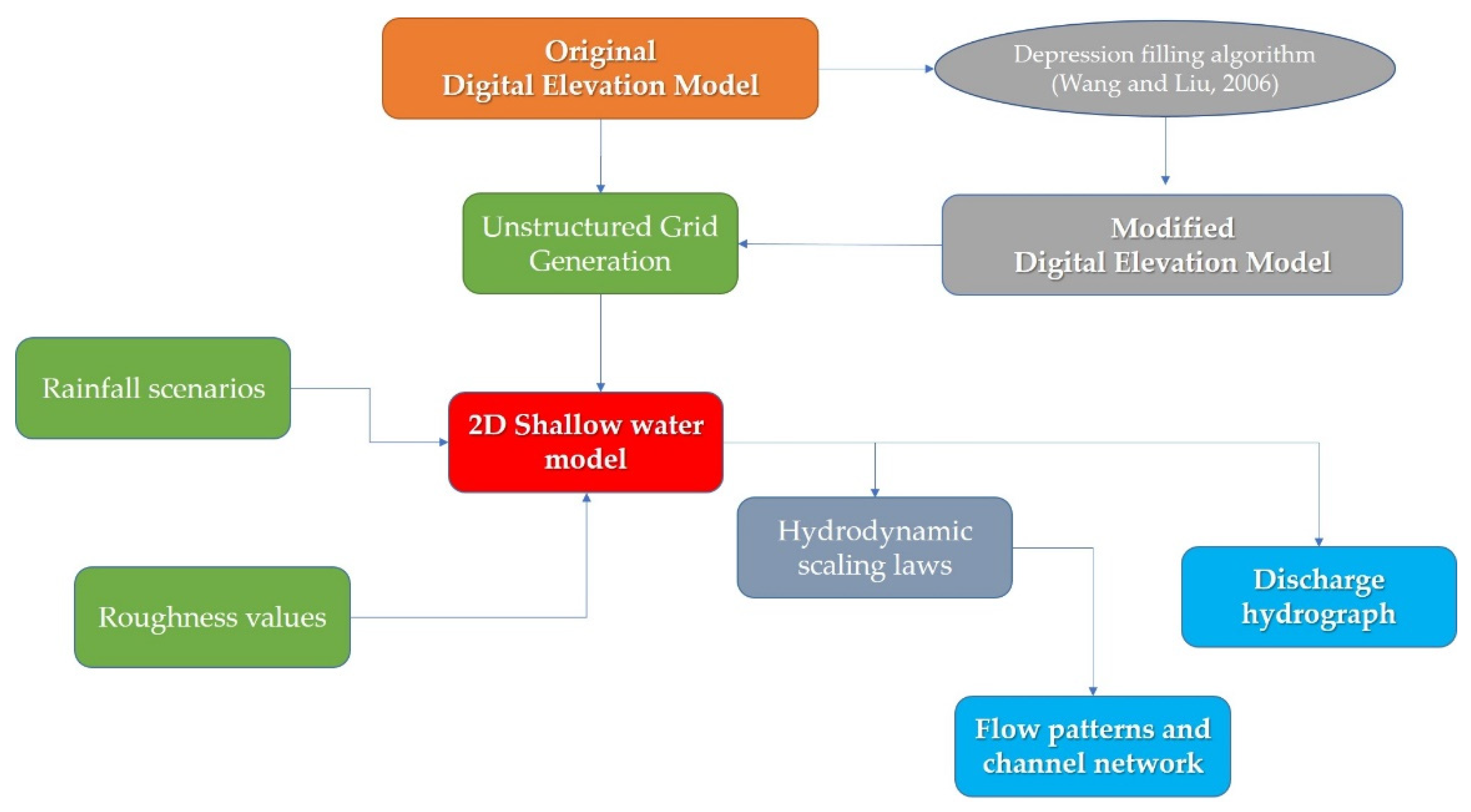
2. Methodological Issues

2.1. 2D SWEs according to the Rainfall-on-Grid Approach and Detection of Flow Patterns

The core of the methodological procedure of this work is based on the use of the 2-D SWEs that can be expressed in the conservative form as reported in Equation (1).

$$\frac{\partial U}{\partial t}+\frac{\partial F}{\partial x}+\frac{\partial G}{\partial y}=S \left(1\right)$$

(1)

where:

$$U=\left(\begin{array}{c}h\\ hu\\ hv\end{array}\right); F=\left(\begin{array}{c}hu\\ h{u}^2+g{h}^2/2\\ huv\end{array}\right); G=\left(\begin{array}{c}hv\\ huv\\ h{v}^2+g{h}^2/2\end{array}\right); S=\left(\begin{array}{c}r-f\\ gh\left(S_{0x}-S_{fx}\right)\\ gh\left(S_{0y}-S_{fy}\right)\end{array}\right)$$

(2)

in which: t is time; x, y are the horizontal coordinates; h is the water depth; u, v are the depth-averaged flow velocities in x- and y- directions; g is the gravitational acceleration; r is the rain intensity and f the infiltration losses; S_0x, S_0y are the bed slopes in x- and y- directions; S_fx, S_fy are the friction slopes in x- and y- directions.

It should be observed that the rainfall supply and the infiltration losses are directly included in the model so that the source term S in the mass continuity equation is different from zero (see Equation (2)). This approach is often identified as direct rainfall method or rain-on-grid approach, since the rain is applied directly onto a two-dimensional grid.

Equation (1) is solved here according to the finite volume method (FVM) approach. Both the numerical schemes and the performances in real cases have been already presented in previous works (i.e., [57,58,59]) and, therefore, are not reported here.

As mentioned before, the approach proposed here is based on the flow patterns tracked by 2D-SWEs simulations. Therefore, following the strategy proposed by [44], the spatial and temporal assessment of both the water depths h and the velocities u,v throughout the basin are obtained by solving Equation (1). Specifically, once obtained the steady state condition for a given rainfall input, the centroid of a given computational cell is considered as “net-point” (and the cell identified as “network cell”) only if the water depth computed in that cell is equal to or greater than of the water depth threshold (h_s).

One of the main results obtained by [44] is the bimodal scaling law that describes the relations between the water depth threshold h_s and the total area of the network cells (A_nc). In particular, once computed, the variable A*, as the ratio between A_nc and total basin area A, the points of coordinates (log h_s, log A*) are arranged according to two linear-like functions characterized by significantly different slopes. The break of the derivative can be used to identify the specific value of h_s that separates flow patterns characterizing the channel network (CN) from those ones related to the hillslope plus channel network (HCN).

Similar behavior has been observed when considering the unit discharges q_s or its dimensionless expression Q* obtained as the ratio between q_s and the unit discharge at the basin outlet Q [45]. It has been shown that the slope of the CN part of the graph can be considered as a morpho-hydrodynamic feature of a natural basin since it provides information related to how much the expansion of the hydrodynamically active areas is associated with an increase in the hydrodynamic variability or, vice versa, how much the hydrodynamic heterogeneity in the channel network is related to an increase in the hydrodynamically active areas.

For all the details, the reader may refer to [44,45]. For the sake of clarity, a typical behavior assumed by these curves is shown in Figure 1. The criterion used for the determination of flow pattern based on these hydrodynamic scaling laws will be identified, hereafter, as ”A*-h_s” and “A*-q_s”curves.

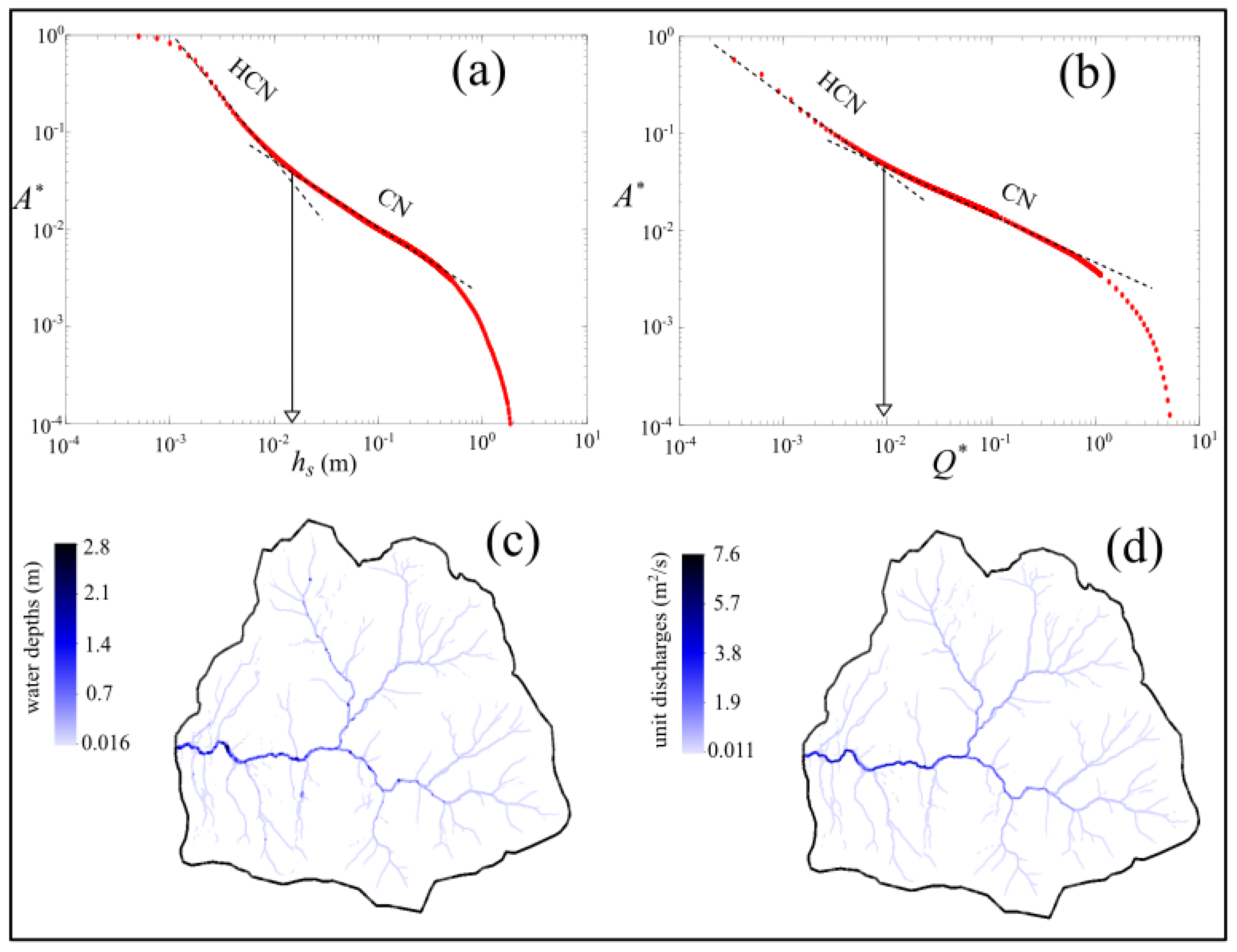
2.2. Hydrodynamic-Based Flow Patterns and Surface Runoff: A Unified Framework

The approach discussed above is used to investigate the effects of the DEM filling on both the flow patterns tracked by 2D SWE modeling and the associated hydrodynamic-hydrologic responses, according to the flow chart depicted in Figure 2.

Specifically, attention is focused on situations of practical interest, for which 1 m or 5 m resolution DEMs are available. These data may be affected by artificial or real depressions that are usually filled for hydrological purposes. The computational grid is generated using both the original DEM (hereafter also identified as “no depression filling”) and the modified one (“depression filling”) according to the well-known algorithm proposed by [29] and available in several GIS environments such as QGIS. The methodology relies on hypothetical scenarios, for which plausible rainfall and roughness values are assumed to initialize the 2D Shallow Water model. The output of the numerical model is based on the hydrodynamic scale laws mentioned above, which represent the criteria used to track the inundation patterns, and the associated discharge hydrographs computed at the basin outlets. Therefore, the overall approach allows us to provide a unified view on both the geometrical features of the river network and the hydrodynamic response of the watersheds in the light of the effects induced by the DEM filling.

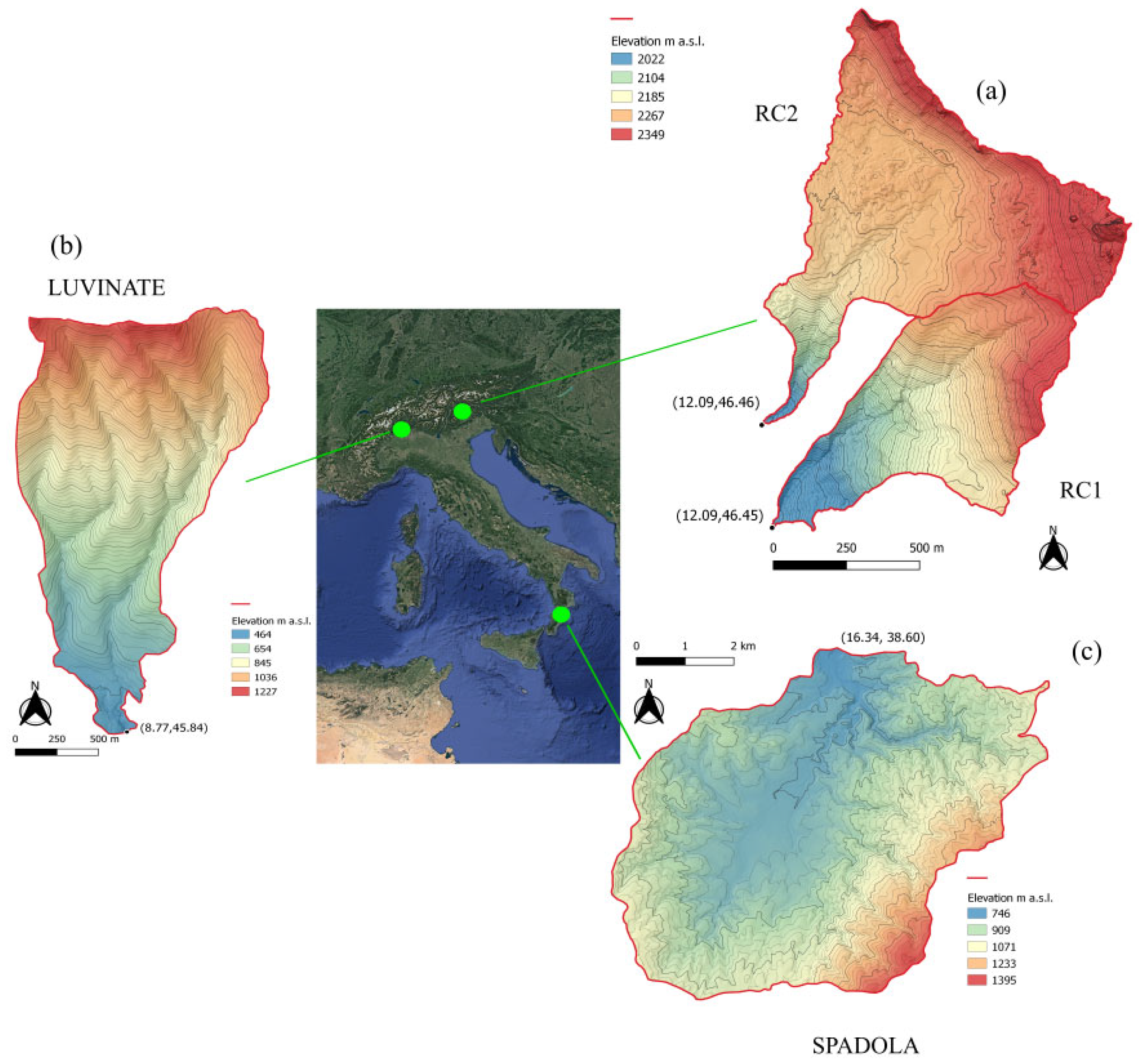
3. Numerical Applications

To evaluate the effects of depression filling in different situations of practical interest, we selected four Italian small basins (see

Table 1. Available data and results of the depression filling algorithm (Wang and Liu, 2006).

Name of Basin	Basin Area (km2)	DEM Resolution (m2)	Filled Volume (m3)	Filled Area (m2)
Luvinate	2.7	25	579	3550
Spadola	45.3	25	340,606	637,075
RC2	0.73	1	29,459	34,448
RC1	0.47	1	186	1229

), for two of which 5 m resolution DEMs were available, while for the remaining two 1 m resolution DEMs were obtained. Very often 5 m resolution DEMs are freely available and considered sufficient for many technical studies, whereas 1 m resolution DEM are used for more detailed analyses. Our purpose, however, is not to discuss the effects of spatial resolution on the depression removal, but to focus on the potential influence that DEM filling could play on the simulated flow patterns and surface runoff in situations of practical interest when analyzing small watersheds, where commonly 1–5 m DEM resolutions are involved.

The 1 m resolution DEMs refer here to two very small catchments, hereafter identified as RC1 and RC2, located in the Italian Eastern Alps and belonging to the Rio Cordon basin. They are shown in Figure 3a, in which the contours lines are plotted every 5 m (bold lines every 25 m). For a detailed description of these basins one may refer to [60,61]. The 5 m resolution DEMs refer to two basins located, respectively, in the Lombardy and Calabria Regions. The first one, hereafter identified as Luvinate, is a part of the Tinella watershed, near the municipality of Luvinate (Varese) and it is shown in Figure 3b (the contour lines are plotted every 10 m with bold lines every 50 m). The second one is a sub-basin of the Ancinale catchment, near the town of Spadola (Vibo Valentia), and it is shown in Figure 3c (the contours lines are plotted every 25 m with bold lines every 100 m). Information related to these catchments can be found, respectively, in [62,63]. The basin areas are reported in Table 1. For all catchments the Wang and Liu (2006) algorithm has been applied to all the selected watersheds. Specifically, some information related to the filling process is reported again in Table 1.

We may assume that the analyzed DEMs describe the hillslope geometries and the river cross sections properly. In particular, as reported by other authors who studied the RC1 and RC2 basins [60], “hillshades of the drainage basins were found to highlight clearly the morphology of channel and, specifically, the heads of these channels”.

For the sake of simplicity, simplified rainfall scenarios have been considered. In particular, constant in time and uniform in space net rain intensities have been assumed (see

Table 2. Simulations and rainfall scenarios.

ID Simulation	Rain Intensity (mm/h)	Rain Duration (min)
Luvinate	14	25
Spadola-1	5	120
Spadola-2	10	120
RC2	15	30
RC1	15	25

), on the basis of available data and observed events [62,64]. Considering the simplified scenario-based approach assumed in this work, plausible rain durations have been deduced from rough estimations of the time of concentration. Spatially variable roughness values should be considered in the modelling, in view of some variability of the land use in the catchments (see, for example, [65]). However, considering that the purpose here is not to reproduce observed events, for the sake of simplicity, we assumed a uniform roughness distribution over the whole catchments, except for the areas covered by the channel network. Therefore, only two values were considered for each catchment, independently from the depression filling process. Expressed roughness in terms of the Manning coefficient, values of 0.03 s∙m^1/3 and 0.06 s∙m^1/3 were adopted for the channel network and the remaining parts of the catchments, respectively.

Finally, for each simulation, we assumed dry conditions everywhere in the computational domain. This implies that the topographic depressions were empty at the beginning of the simulations. The boundary conditions used for all the simulations refer to a transmissive condition (open boundary) near the basin outlets and a solid wall boundary condition on the watershed divide.

4. Results and Discussion

4.1. Analysis of 5 m Resolution DEMs

As for the simulation “Luvinate-1”, using the methodology depicted in Figure 2, we obtained the bimodal scaling laws shown in Figure 4a,b, considering the impact of the depression filling process.

In this situation, no difference appears in the HCN part of the curves and only slight modifications exist on the CN side. This means the geomorphic structure of the river network is substantially similar.

This fact is highlighted in Figure 5, in which the drainage patterns tracked by the 2D-SWEs model, using the two different criteria, are compared considering both the original and filled DEM. Figure 5 further shows that the two criteria for the extraction of the drainage patterns are substantially equivalent, being the difference among the simulated networks negligible.

The effect of the DEM filling has some influence on the distribution of the water depth throughout the domain, leading to local differences in their values, especially in the downstream part of the watershed, as highlighted by the contour maps shown in Figure 5. As a consequence, some slight effects of the simulated discharge are expected (see Figure 4c). In particular, the computed discharge at the basin outlet is slightly faster than that related to the original DEM and the peak value is a little bit higher. The difference in the outflow volume may be easily explained by the greater stored water volume in the case of the simulation related to the original DEM. However, these differences can be considered as not particularly important.

Figure 6 shows the effects of the depression filling on the A*-h_s curve obtained for the Spadola watershed, considering both the simulations described in Table 2. For both the situations, no difference appears in the HCN part of the curves whereas some variations can be observed on the CN side of the curve that can be appreciated, especially for the higher value of h_s. Specifically, these differences seem to be more pronounced for the simulation “Spadola-1” (Figure 6a), related to the lower rainfall intensity.

The variations observed for higher water depths highlight the different hydrodynamic behavior induced by the depression filling that can impact on the estimation of the discharge hydrographs, as shown in Figure 7. In particular, significant differences appear in arrival times, peak discharge, hydrograph shape and flood volumes. These discrepancies seem to be amplified in the scenario related to the lower rainfall intensity “Spadola-1”.

The overall behavior described by the A*-h_s curves suggests similar geomorphic structures of the river network, confirmed by the flow patterns shown in Figure 8.

4.2. Analysis of 1 m Resolution DEMs

The two scaling laws related to the original and filled DEM, obtained for this application, are shown in Figure 9a,b. No differences appear in the HCN part of the curves and only slight modifications exist on the CN side. In particular, the A*-q_s curve seems to be not affected by the DEM filling.

Therefore, also in this case, the geomorphic structure of the river network is expected to be very similar. As can be observed from Figure 10, the two networks extracted using the A*-q_s* scaling law are very similar (the networks tracked by the A*-h_s criterion are not shown as they are practically the same). Figure 10 also highlights the good ability of the flow patterns tracked by the 2D SWEs model in the detection of the observed channel heads locations (circles), for both the simulations related to the original and modified DEMs. Moreover, the hydrodynamic drainage patterns show a level of accuracy similar to the channel network (black line) extracted by the method that gave the best performances among those ones analyzed in [61], based on this case on the computations of the Strahler classification of surface flow paths and pruning the exterior link. In particular, it seems that the occurrence of channel locations, where channels are not observed, is lower using the hydrodynamic-based method considered in this work.

Finally, the discharge hydrograph simulated using this scenario seems not to be significantly affected by the depression filling process (Figure 9c). In this case, only a slight reduction in the peak value can be observed together with some effects during the recession limb of the hydrograph due to the modification in the storage volume inside the watershed.

A very different behavior is observed for the RC2 basin (Figure 11). Specifically, as shown in Figure 11a, the A*-h_s curves generated by the 2D-SWEs model show significant variations between each other, leading to a different spatial distribution of the water depth values throughout the watershed. In particular, the CN part of the graph is drastically affected by the depression filling process, leading to a significant modification of the slope that characterizes the original DEM. This means that the flow patterns characterizing the channel networks have different geomorphological features. This is confirmed by Figure 12, in which the two networks tracked by the A*-h_s criterion are shown together with the location of the observed channel heads.

All the methods considered in [61] overestimated the extension of the CN in the NW part of the drainage basin, where channels are not observed to occur. In any case, in that paper, it is reported that the method that uses a threshold on the function AS², in which A is the drainage area and S the local slope, provided the best results since it did not reproduce a clear CN in the NW part of the basin. This solution has been reproduced in Figure 12 (black lines) for comparative purposes.

The network simulated using the original DEM (Figure 12a) shows the tendency to detect channel heads positions where channels have been really observed. As regards the NW part of the basin, the flow patterns corresponding to the selected threshold do not represent a clear channel network, configuring quite fragmented flow connectivity. This behavior has been significantly altered by the depression filling process (Figure 12b), so that artificial flow patterns were generated (see, for example, the blue arrows in Figure 12b).

In a situation like this, the watershed response to a storm event is expected to be very different, as confirmed in Figure 11b. The discharge hydrograph simulated using the DEM, after the depression filling, shows significant differences in terms of peak value and flood volume in respect to the simulation related to the original DEM.

5. Discussion

The results shown in the previous section highlight that the influence of DEM depression filling, on both the structure of the hydrodynamic patterns and the associated discharge hydrograph, may be important or not. On the other hand, the results related to the Spadola watershed highlighted that the depression filling effects depend on the rainfall scenario assumed to initialize the 2D SWEs model. Therefore, to better analyze the results as a whole, it seems interesting to interpret all the simulations in light of the ratio between the fillable volume F_V (see Table 2) and the rainfall inflow volumes R_V, hereafter identified as IFR (see Equation (3)).

$$\mathrm{IFR}=\frac{F_V}{R_V}$$

(3)

The values of this ratio are reported in

Table 3. Summary of the values related to IOV and IFR for each simulation.

Simulation	IOV (-)	IFR (-)
Luvinate	0.02	0.04
Spadola-1	0.59	0.75
Spadola-2	0.25	0.38
RC2	0.54	5.4
RC1	0.05	0.065

, together with an index of outflow volume variation, hereafter identified as IOV, defined as in Equation (4):

$$\mathrm{IOV}=\frac{V_F-V_{NF}}{V_{NF}}$$

(4)

where V_F and V_NF are the volumes of the discharge hydrographs computed, respectively, with and without depression filling at the basin outlets.

Table 3 highlights that the value of the IFR index is very low when the effects of the depression filling is negligible or, in other terms, the IOV is very low (Luvinate and RC1 simulations). Looking at values related to the Spadola watershed, the halving of the IFR index leads to a reduction in terms of IOV of a factor 2. Finally, it is interesting to underline the very high value assumed by IFR in the case of RC2 simulation, for which significant differences in terms of flow pattern structures have been observed.

As highlighted by Table 3, as IFR increases IOV increases too. Specifically, if attention is strictly focused on the simulation, for which IOV < 1 (RC2 is excluded), the relation is substantially linear. Indeed, the situation related to RC2 simulation seems to be an extreme case, characterized by a very high fillable volume. However, the number of simulations considered in this work are not enough to derive a meaningful relation between the two indexes IFR and IOV. Moreover, the IFR values may also be affected by the different resolutions of DEMs. Finally, it is reasonable to assume that the ratio between the basin area and the DEM resolution might influence the IFR values.

The IFR index alone cannot describe the spatial distribution of the filled volume, which it is expected to significantly influence the results. However, a clear tendency appears in the results so that the IFR index might be seen, at least, as a preliminary and rough measure of the effects induced by the depression filling on the modelling results.

Potential Impact of the Research and Future Works

Depressions in DEMs have been traditionally seen as a feature to remove as the flow is trapped, and thus, no outward flow direction is available to route and accumulate the flows. Therefore, to simplify hydrologic analysis for practical purposes, the common approach treated all depressions in DEMs as artefacts and completely removed them in the DEM data preprocessing prior to modelling.

This paper provided a novel point of view related to the traditional procedure of depression filling in DEMs. As a matter of principle, there is no need to apply the available depression filling algorithm to both track flow patterns and compute the watershed response to rain events using the 2D SWEs modeling. For this reason, this approach has the potential to analyze the effects induced by depression filling in the hydrological and geomorphologic analyses at the watershed-scale.

This paper has been mainly focused on DEM resolutions of practical interest, for which a lot of data are available and freely shared. In this context, the observed difference in terms of outflow volumes and arrival times may be easily explained by the greater stored water volume in the case of the simulation related to the use of the original DEM. However, this behavior should be analyzed in the light of the role of the contrasting roughness of the overland and channel flow paths that may induce similar effects. Therefore, the combined analysis of depression filling and roughness estimation might represent an interesting development of this research.

Further advances in this research may be represented by the analysis of the depression filling effects on the simulated hydrographs and flow patterns as a function of the rain features (return period, duration etc.). Such a careful investigation would require a paper in itself and, therefore, it cannot be faced in this work.

Mostly, the methodological framework presented in this work may contribute to develop methods and tools for the analysis of topographic depressions in high-resolution elevation data and their influence on river network connectivity and in watershed-scale modeling, feeding the debate within the literature referred to in the introduction.

6. Conclusions

The 2D SWEs model used according to the rain on grid approach proved to be an effective tool for the analysis of the effects induced by depression filling on both the channel network structure and the discharge hydrograph simulated at the watershed outlets. Several simulations on different basins have been carried out in order to understand how important these effects might be in practical applications. The experience gained in this work can be summarized as follows.

(1)

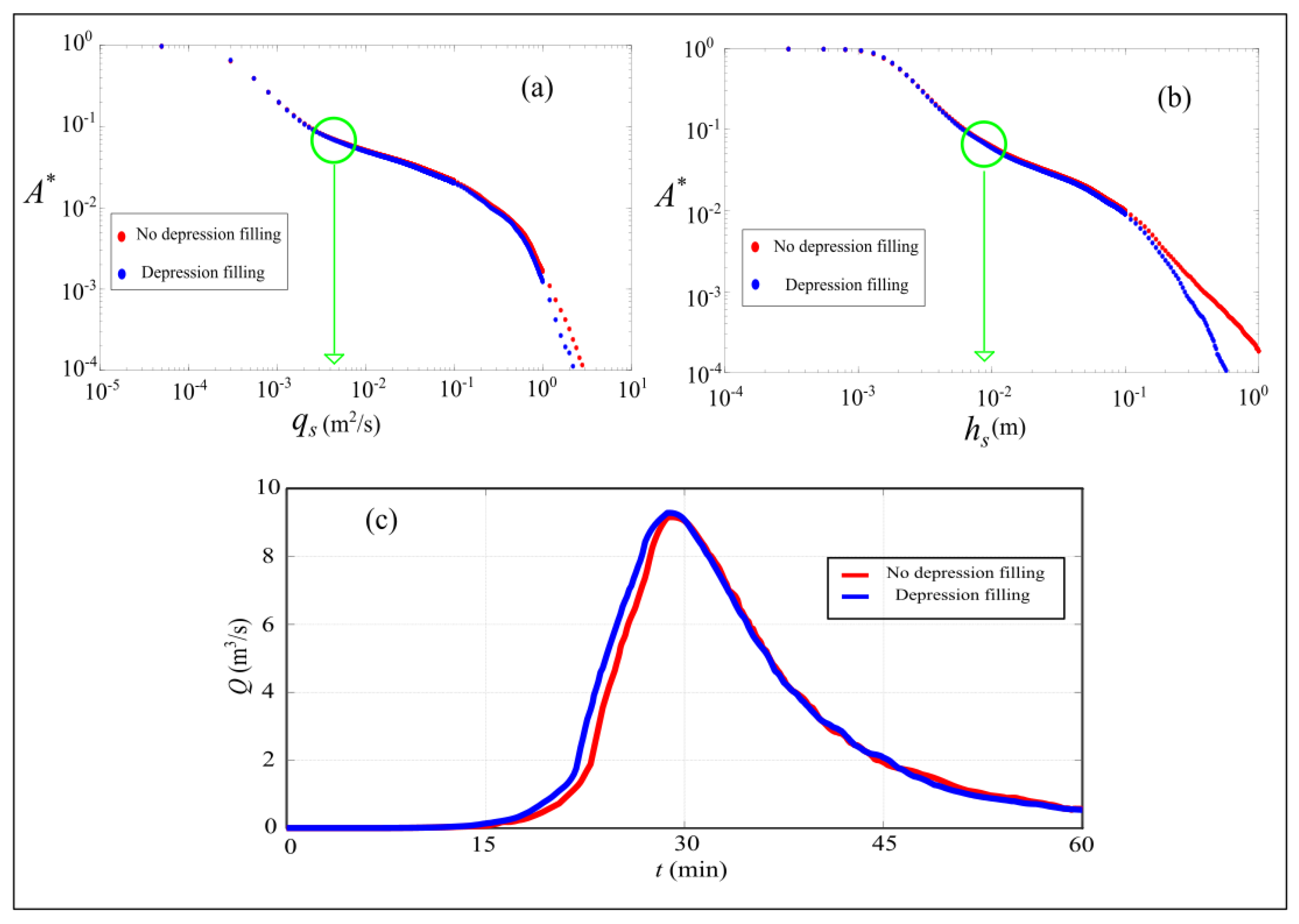
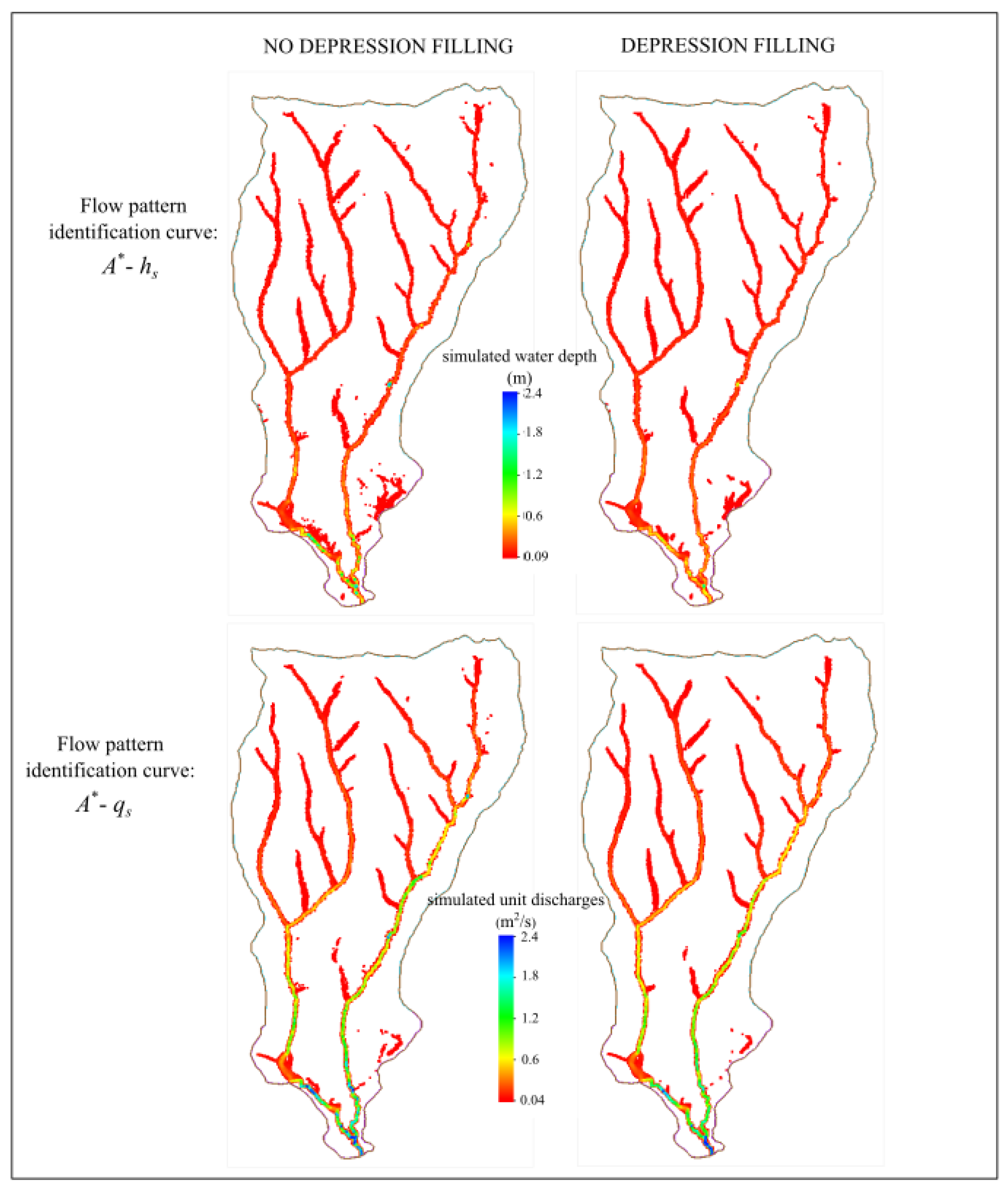
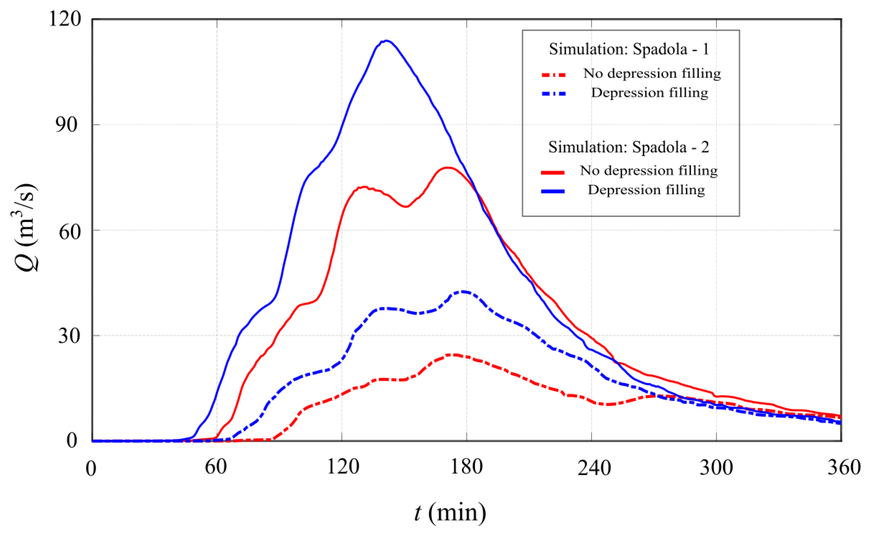
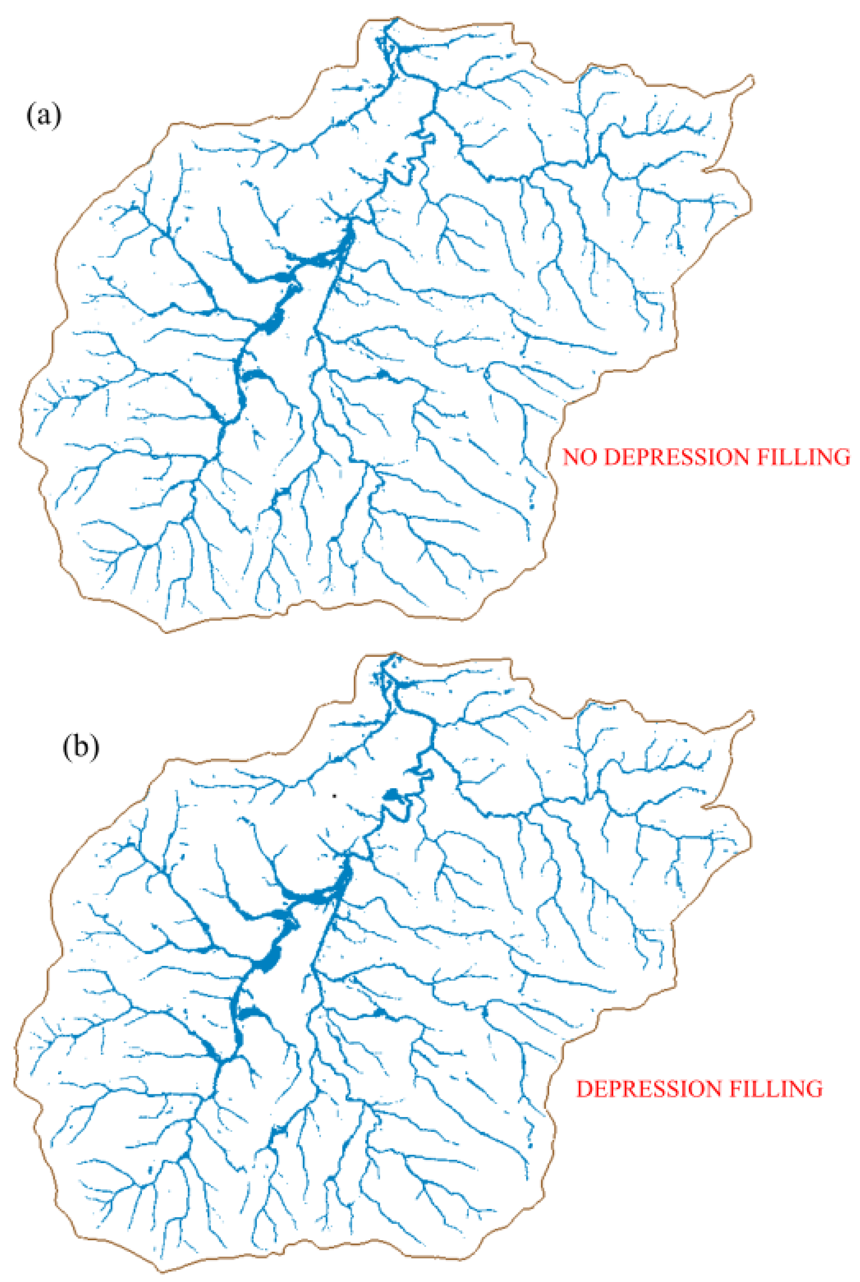
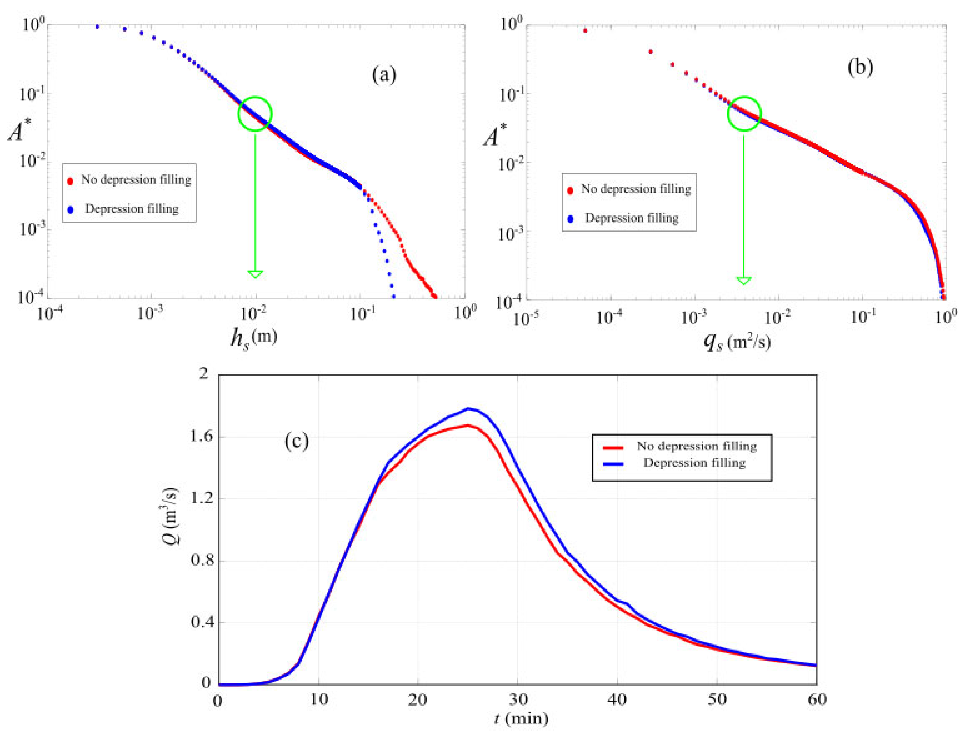
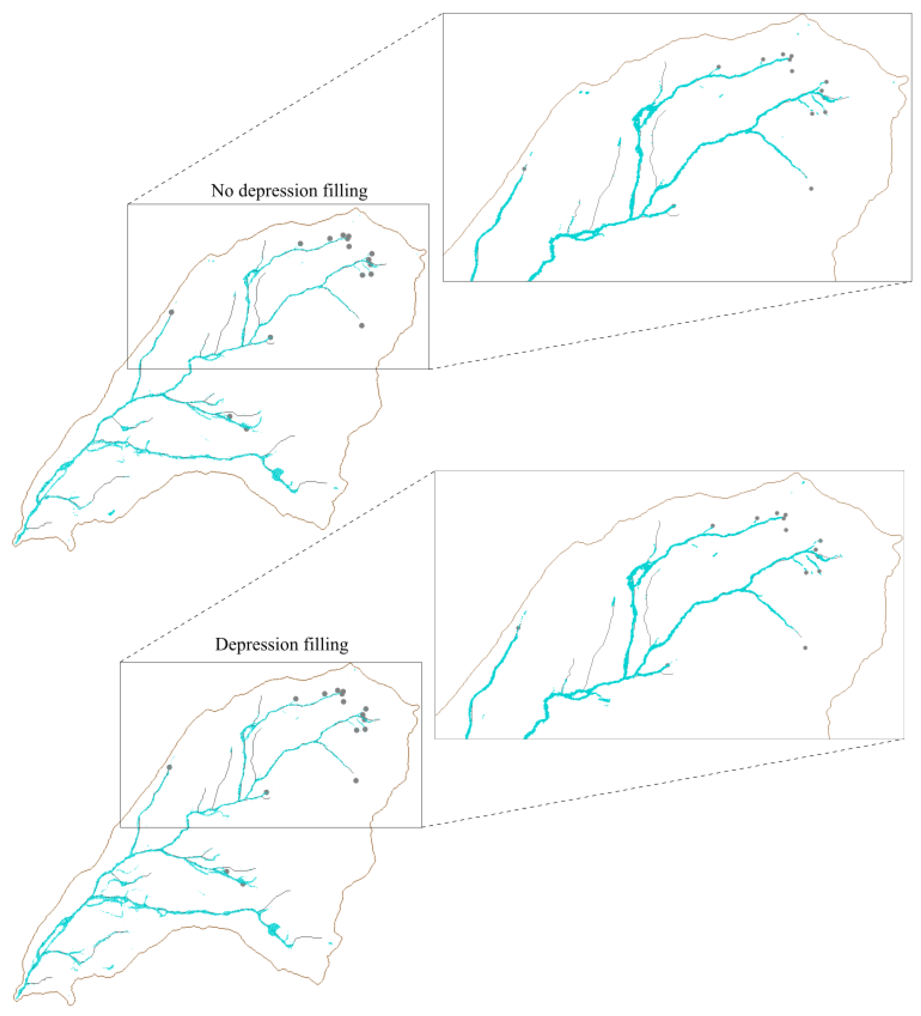
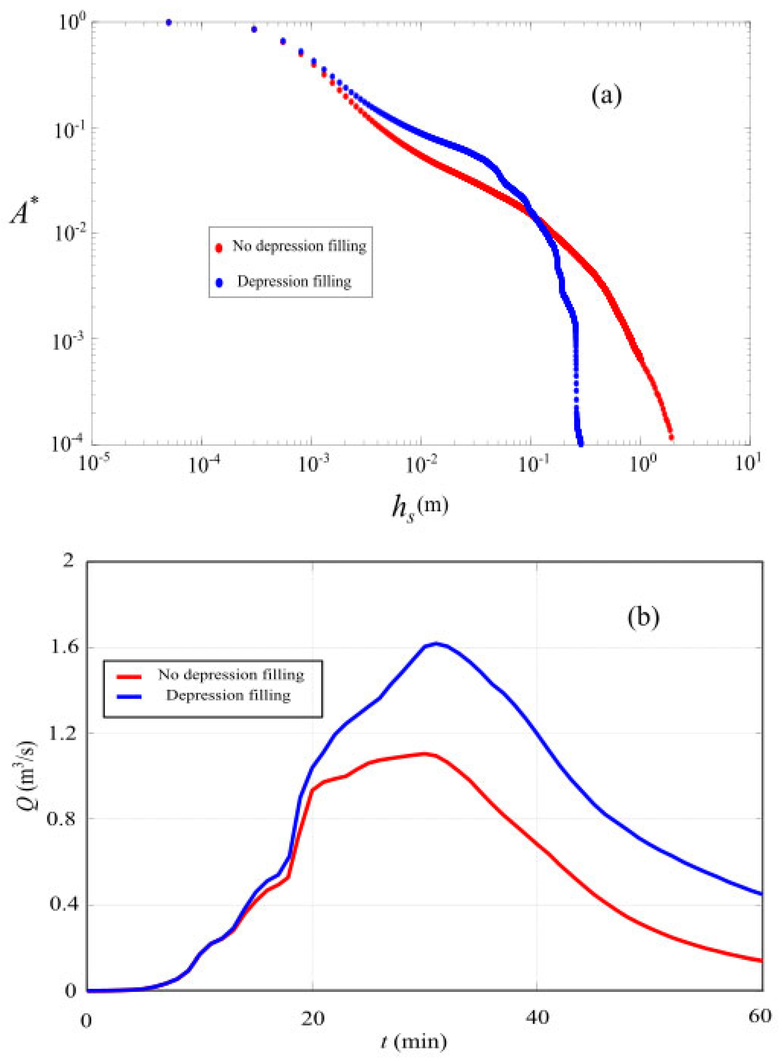
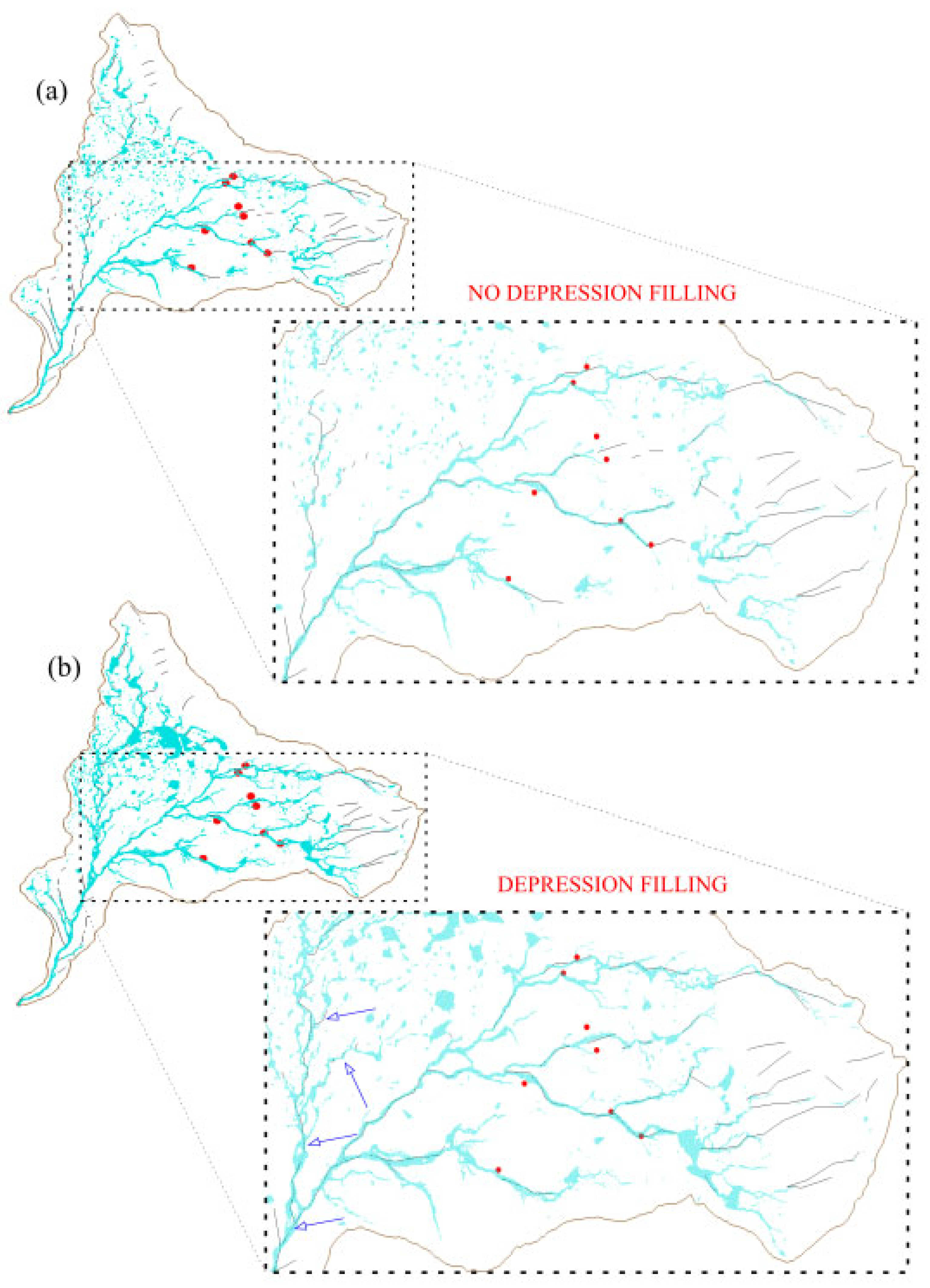
The effects of the depression filling on the flow patterns and discharge hydrographs should be evaluated case to case. In a couple of situations, no significant differences have been observed in terms of simulated discharge hydrographs and geomorphic structure of the channel network. However, it has been shown that depression filling algorithms may lead to significant alterations of the flow patterns, detected by the hydrodynamic laws, generating also significant variations in the simulated hydrographs. Therefore, this occurrence should be taken into account when applying this type of algorithm;

(2)

The effects of the depression filling algorithm should be considered in light of the rainfall scenario. In this context, the IFR index introduced in this work seems to represent a practical and expeditious way to preliminarily assess the potential influence of DEM depression filling on the simulation results for a given event.

Further studies and analysis are needed to provide more general conclusions on the issues faced in this work.

References

1. Gandolfi, C.; Bischetti, G.B. Influence of the drainage network identification method on geomorphological properties and hydrological response. Hydrol. Process. 1997, 11, 353–375. [Google Scholar] [CrossRef]
2. Benda, L.; Poff, N.L.; Miller, D.; Dunne, T.; Reeves, G.; Pess, G.; Pollock, M. The Network Dynamics Hypothesis: How Channel Networks Structure Riverine Habitats. Bioscience 2004, 54, 413–427. [Google Scholar] [CrossRef] [Green Version]
3. Rodriguez-Iturbe, I.; Muneepeerakul, R.; Bertuzzo, E.; Levin, S.; Rinaldo, A. River networks as ecological corridors: A complex systems perspective for integrating hydrologic, geomorphologic, and ecologic dynamics. Water Resour. Res. 2009, 45. [Google Scholar] [CrossRef]
4. Zaliapin, I.; Foufoula-Georgiou, E.; Ghil, M. Transport on river networks: A dynamic tree approach. J. Geophys. Res. Earth Surf. 2010, 115. [Google Scholar] [CrossRef] [Green Version]
5. Millares, A.; Gulliver, Z.; Polo, M. Scale effects on the estimation of erosion thresholds through a distributed and physically-based hydrological model. Geomorphology 2012, 153–154, 115–126. [Google Scholar] [CrossRef]
6. Buchanan, B.P.; Archibald, J.A.; Easton, Z.M.; Shaw, S.B.; Schneider, R.L.; Walter, M.T. A phosphorus index that combines critical source areas and transport pathways using a travel time approach. J. Hydrol. 2013, 486, 123–135. [Google Scholar] [CrossRef]
7. Czuba, J.A.; Foufoula-Georgiou, E. Dynamic connectivity in a fluvial network for identifying hotspots of geomorphic change. Water Resour. Res. 2015, 51, 1401–1421. [Google Scholar] [CrossRef]
8. Bai, R.; Li, T.; Huang, Y.; Li, J.; Wang, G. An efficient and comprehensive method for drainage network extraction from DEM with billions of pixels using a size-balanced binary search tree. Geomorphology 2015, 238, 56–67. [Google Scholar] [CrossRef]
9. Choi, Y. A new algorithm to calculate weighted flow-accumulation from a DEM by considering surface and underground stormwater infrastructure. Environ. Model. Softw. 2012, 30, 81–91. [Google Scholar] [CrossRef]
10. Li, J.; Li, T.; Zhang, L.; Sivakumar, B.; Fu, X.; Huang, Y.; Bai, R. A D8-compatible high-efficient channel head recognition method. Environ. Model. Softw. 2020, 125, 104624. [Google Scholar] [CrossRef]
11. Orlandini, S.; Moretti, G. Determination of surface flow paths from gridded elevation data. Water Resour. Res. 2009, 45. [Google Scholar] [CrossRef] [Green Version]
12. O’Callaghan, J.F.; Mark, D.M. The extraction of drainage networks from digital elevation data. Comput. Vis. Graph. Image Process. 1984, 28, 323–344. [Google Scholar] [CrossRef]
13. Wu, T.; Li, J.; Li, T.; Sivakumar, B.; Zhang, G.; Wang, G. High-efficient extraction of drainage networks from digital elevation models constrained by enhanced flow enforcement from known river maps. Geomorphology 2019, 340, 184–201. [Google Scholar] [CrossRef]
14. Montgomery, D.R.; Dietrich, W.E. Source areas, drainage density, and channel initiation. Water Resour. Res. 1989, 25, 1907–1918. [Google Scholar] [CrossRef] [Green Version]
15. Tarboton, D.G.; Bras, R.L.; Rodriguez-Iturbe, I. On the extraction of channel networks from digital elevation data. Hydrol. Process. 1991, 5, 81–100. [Google Scholar] [CrossRef]
16. Tarboton, D.G. A new method for the determination of flow directions and upslope areas in grid digital elevation models. Water Resour. Res. 1997, 33, 309–319. [Google Scholar] [CrossRef] [Green Version]
17. Lacroix, M.P.; Martz, L.W.; Kite, G.W.; Garbrecht, J. Using digital terrain analysis modeling techniques for the parameterization of a hydrologic model. Environ. Model. Softw. 2002, 17, 125–134. [Google Scholar] [CrossRef]
18. Shelef, E.; Hilley, G.E. Impact of flow routing on catchment area calculations, slope estimates, and numerical simulations of landscape development. J. Geophys. Res. Earth Surf. 2013, 118, 2105–2123. [Google Scholar] [CrossRef]
19. Passalacqua, P.; Belmont, P.; Staley, D.M.; Simley, J.D.; Arrowsmith, J.R.; Bode, C.A.; Crosby, C.; DeLong, S.B.; Glenn, N.F.; Kelly, S.A.; et al. Analyzing high resolution topography for advancing the understanding of mass and energy transfer through landscapes: A review. Earth Sci. Rev. 2015, 148, 174–193. [Google Scholar] [CrossRef] [Green Version]
20. Tarolli, P. High-resolution topography for understanding Earth surface processes: Opportunities and challenges. Geomorphology 2014, 216, 295–312. [Google Scholar] [CrossRef]
21. Zheng, X.; Godbout, L.; Zheng, J.; McCormick, C.; Passalacqua, P. An automatic and objective approach to hydro-flatten high resolution topographic data. Environ. Model. Softw. 2019, 116, 72–86. [Google Scholar] [CrossRef]
22. Hiatt, M.; Sonke, W.; Addink, E.A.; van Dijk, W.M.; van Kreveld, M.; Ophelders, T.; Verbeek, K.; Vlaming, J.; Speckmann, B.; Kleinhans, M.G. Geometry and Topology of Estuary and Braided River Channel Networks Automatically Extracted from Topographic Data. J. Geophys. Res. Earth Surf. 2020, 125, e2019JF005206. [Google Scholar] [CrossRef] [PubMed] [Green Version]
23. Arnold, N. A new approach for dealing with depressions in digital elevation models when calculating flow accumulation values. Prog. Phys. Geogr. Earth Environ. 2010, 34, 781–809. [Google Scholar] [CrossRef]
24. Hutchinson, M. A new procedure for gridding elevation and stream line data with automatic removal of spurious pits. J. Hydrol. 1989, 106, 211–232. [Google Scholar] [CrossRef]
25. Wechsler, S.P. Uncertainties associated with digital elevation models for hydrologic applications: A review. Hydrol. Earth Syst. Sci. 2007, 11, 1481–1500. [Google Scholar] [CrossRef] [Green Version]
26. Lindsay, J.B.; Creed, I.F. Removal of artifact depressions from digital elevation models: Towards a minimum impact approach. Hydrol. Process. 2005, 19, 3113–3126. [Google Scholar] [CrossRef]
27. Vaze, J.; Teng, J.; Spencer, G. Impact of DEM accuracy and resolution on topographic indices. Environ. Model. Softw. 2010, 25, 1086–1098. [Google Scholar] [CrossRef]
28. Jenson, S.K.; Domingue, J.O. Extracting Topographic Structure from Digital Elevation Data for Geographic Information System Analysis. Photogramm. Eng. Remote Sens. 1988, 54, 1593–1600. [Google Scholar]
29. Wang, L.; Liu, H. An efficient method for identifying and filling surface depressions in digital elevation models for hydrologic analysis and modelling. Int. J. Geogr. Inf. Sci. 2006, 20, 193–213. [Google Scholar] [CrossRef]
30. Barnes, R.; Lehman, C.; Mulla, D. Priority-flood: An optimal depression-filling and watershed-labeling algorithm for digital elevation models. Comput. Geosci. 2014, 62, 117–127. [Google Scholar] [CrossRef] [Green Version]
31. Soille, P. Optimal removal of spurious pits in grid digital elevation models. Water Resour. Res. 2004, 40. [Google Scholar] [CrossRef] [Green Version]
32. Wang, Y.-J.; Qin, C.-Z.; Zhu, A.-X. Review on algorithms of dealing with depressions in grid DEM. Ann. GIS 2019, 25, 83–97. [Google Scholar] [CrossRef] [Green Version]
33. Wei, H.; Zhou, G.; Fu, S. Efficient Priority-Flood depression filling in raster digital elevation models. Int. J. Digit. Earth 2019, 12, 415–427. [Google Scholar] [CrossRef]
34. Chen, B.; Ma, C.; Xiao, Y.; Gao, H.; Shi, P.; Zheng, J. Retaining Relative Height Information: An Enhanced Technique for Depression Treatment in Digital Elevation Models. Water 2021, 13, 3347. [Google Scholar] [CrossRef]
35. Hou, J.; Li, X.; Pan, Z.; Wang, J.; Wang, R. Effect of digital elevation model spatial resolution on depression storage. Hydrol. Process. 2021, 35, e14381. [Google Scholar] [CrossRef]
36. Rajib, A.; Golden, H.E.; Lane, C.R.; Wu, Q. Surface Depression and Wetland Water Storage Improves Major River Basin Hydrologic Predictions. Water Resour. Res. 2020, 56, e2019WR026561. [Google Scholar] [CrossRef]
37. Woodrow, K.; Lindsay, J.B.; Berg, A.A. Evaluating DEM conditioning techniques, elevation source data, and grid resolution for field-scale hydrological parameter extraction. J. Hydrol. 2016, 540, 1022–1029. [Google Scholar] [CrossRef]
38. Yu, F.; Harbor, J.M. The effects of topographic depressions on multiscale overland flow connectivity: A high-resolution spatiotemporal pattern analysis approach based on connectivity statistics. Hydrol. Process. 2019, 33, 1403–1419. [Google Scholar] [CrossRef]
39. O’Neil, G.L.; Saby, L.; Band, L.E.; Goodall, J.L. Effects of LiDAR DEM Smoothing and Conditioning Techniques on a Topography-Based Wetland Identification Model. Water Resour. Res. 2019, 55, 4343–4363. [Google Scholar] [CrossRef]
40. Hu, L.; Bao, W.; Shi, P.; Wang, J.; Lu, M. Simulation of overland flow considering the influence of topographic depressions. Sci. Rep. 2020, 10, 6128. [Google Scholar] [CrossRef]
41. Zeng, L.; Chu, X. Integrating depression storages and their spatial distribution in watershed-scale hydrologic modeling. Adv. Water Resour. 2021, 151, 103911. [Google Scholar] [CrossRef]
42. Limaye, A.B. Extraction of Multithread Channel Networks with a Reduced-Complexity Flow Model. J. Geophys. Res. Earth Surf. 2017, 122, 1972–1990. [Google Scholar] [CrossRef]
43. Davy, P.; Croissant, T.; Lague, D. A precipiton method to calculate river hydrodynamics, with applications to flood prediction, landscape evolution models, and braiding instabilities. J. Geophys. Res. Earth Surf. 2017, 122, 1491–1512. [Google Scholar] [CrossRef] [Green Version]
44. Costabile, P.; Costanzo, C.; De Bartolo, S.; Gangi, F.; Macchione, F.; Tomasicchio, G.R. Hydraulic Characterization of River Networks Based on Flow Patterns Simulated by 2-D Shallow Water Modeling: Scaling Properties, Multifractal Interpretation, and Perspectives for Channel Heads Detection. Water Resour. Res. 2019, 55, 7717–7752. [Google Scholar] [CrossRef]
45. Costabile, P.; Costanzo, C. A 2D-SWEs framework for efficient catchment-scale simulations: Hydrodynamic scaling properties of river networks and implications for non-uniform grids generation. J. Hydrol. 2021, 599, 126306. [Google Scholar] [CrossRef]
46. Stanislawski, L.; Shavers, E.; Wang, S.; Jiang, Z.; Usery, E.; Moak, E.; Duffy, A.; Schott, J. Extensibility of U-Net Neural Network Model for Hydrographic Feature Extraction and Implications for Hydrologic Modeling. Remote Sens. 2021, 13, 2368. [Google Scholar] [CrossRef]
47. Fernández-Pato, J.; Morales-Hernández, M.; García-Navarro, P. Implicit finite volume simulation of 2D shallow water flows in flexible meshes. Comput. Methods Appl. Mech. Eng. 2018, 328, 1–25. [Google Scholar] [CrossRef] [Green Version]
48. Lacasta, A.; Hernández, M.M.; Murillo, J.; García-Navarro, P. GPU implementation of the 2D shallow water equations for the simulation of rainfall/runoff events. Environ. Earth Sci. 2015, 74, 7295–7305. [Google Scholar] [CrossRef]
49. Juez, C.; Lacasta, A.; Murillo, J.; García-Navarro, P. An efficient GPU implementation for a faster simulation of unsteady bed-load transport. J. Hydraul. Res. 2016, 54, 275–288. [Google Scholar] [CrossRef]
50. Xia, X.; Liang, Q.; Ming, X. A full-scale fluvial flood modelling framework based on a high-performance integrated hydrodynamic modelling system (HiPIMS). Adv. Water Resour. 2019, 132, 103392. [Google Scholar] [CrossRef]
51. Aureli, F.; Prost, F.; Vacondio, R.; Dazzi, S.; Ferrari, A. A GPU-Accelerated Shallow-Water Scheme for Surface Runoff Simulations. Water 2020, 12, 637. [Google Scholar] [CrossRef] [Green Version]
52. Ming, X.; Liang, Q.; Xia, X.; Li, D.; Fowler, H.J. Real-Time Flood Forecasting Based on a High-Performance 2-D Hydrodynamic Model and Numerical Weather Predictions. Water Resour. Res. 2020, 56, e2019WR025583. [Google Scholar] [CrossRef]
53. Özgen, I.; Teuber, K.; Simons, F.; Liang, D.; Hinkelmann, R. Upscaling the shallow water model with a novel roughness formulation. Environ. Earth Sci. 2015, 74, 7371–7386. [Google Scholar] [CrossRef]
54. Caviedes-Voullième, D.; García-Navarro, P.; Murillo, J. Influence of mesh structure on 2D full shallow water equations and SCS Curve Number simulation of rainfall/runoff events. J. Hydrol. 2012, 448–449, 39–59. [Google Scholar] [CrossRef]
55. Fernández-Pato, J.; García-Navarro, P. 2D Zero-Inertia Model for Solution of Overland Flow Problems in Flexible Meshes. J. Hydrol. Eng. 2016, 21, 04016038. [Google Scholar] [CrossRef]
56. Caviedes-Voullième, D.; Ahmadinia, E.; Hinz, C. Interactions of Microtopography, Slope and Infiltration Cause Complex Rainfall-Runoff Behavior at the Hillslope Scale for Single Rainfall Events. Water Resour. Res. 2021, 57, e2020WR028127. [Google Scholar] [CrossRef]
57. Padulano, R.; Costabile, P.; Costanzo, C.; Rianna, G.; Del Giudice, G.; Mercogliano, P. Using the present to estimate the future: A simplified approach for the quantification of climate change effects on urban flooding by scenario analysis. Hydrol. Process. 2021, 35, e14436. [Google Scholar] [CrossRef]
58. Costabile, P.; Costanzo, C.; Ferraro, D.; Barca, P. Is HEC-RAS 2D accurate enough for storm-event hazard assessment? Lessons learnt from a benchmarking study based on rain-on-grid modelling. J. Hydrol. 2021, 603, 126962. [Google Scholar] [CrossRef]
59. Costabile, P.; Costanzo, C.; De Lorenzo, G.; De Santis, R.; Penna, N.; Macchione, F. Terrestrial and airborne laser scanning and 2-D modelling for 3-D flood hazard maps in urban areas: New opportunities and perspectives. Environ. Model. Softw. 2021, 135, 104889. [Google Scholar] [CrossRef]
60. De Bartolo, S.; Dell’Accio, F.; Frandina, G.; Moretti, G.; Orlandini, S.; Veltri, M. Relation between grid, channel, and Peano networks in high-resolution digital elevation models. Water Resour. Res. 2016, 52, 3527–3546. [Google Scholar] [CrossRef] [Green Version]
61. Orlandini, S.; Tarolli, P.; Moretti, G.; Fontana, G.D. On the prediction of channel heads in a complex alpine terrain using gridded elevation data. Water Resour. Res. 2011, 47. [Google Scholar] [CrossRef] [Green Version]
62. Folador, L.; Cislaghi, A.; Vacchiano, G.; Masseroni, D. Integrating Remote and In-Situ Data to Assess the Hydrological Response of a Post-Fire Watershed. Hydrology 2021, 8, 169. [Google Scholar] [CrossRef]
63. Barbero, G.; Costabile, P.; Costanzo, C.; Ferraro, D.; Petaccia, G. 2D Hydrodynamic Approach Supporting Evaluations of Hydrological Response in Small Watersheds: Implications for Lag Time Estimation. J. Hydrol. 2022. under second review. [Google Scholar]
64. Lenzi, M.A. Step-pool evolution in the Rio Cordon, northeastern Italy. Earth Surf. Process. Landf. 2001, 26, 991–1008. [Google Scholar] [CrossRef]
65. Costabile, P.; Macchione, F.; Natale, L.; Petaccia, G. Flood mapping using LIDAR DEM. Limitations of the 1-D modeling highlighted by the 2-D approach. Nat. Hazards 2015, 77, 181–204. [Google Scholar] [CrossRef]
Figure 1. Typical profiles characterizing the A*-hs and A*-Q* curve (a,b) and the associated drainage patterns associated to the values of hs and Q* estimated in the part of the curves, in which the break of derivative occur (c,d), (from Costabile and Costanzo, 2021, modified).
Water 14 00997 g001
Figure 2. Flow chart illustrating the methodology used in this work.
Water 14 00997 g002
Figure 3. Catchments considered in this work and geographical coordinates (WGS84) of the outlet sections. A 1 m resolution DEM is available for RC1 and RC2 basins (a) whereas a 5 m resolution DEM is available for Luvinate (b) and Spadola (c).
Water 14 00997 g003
Figure 4. Luvinate watershed: effects of the depression filling on both the A*-qs (a) and A*-hs (b) curves and the simulated discharges (c).
Water 14 00997 g004
Figure 5. Luvinate watersed: effects of the DEM filling on the river drainage patterns tracked by the rain-on-grid approach using the bimodal scaling laws criteria.
Water 14 00997 g005
Figure 6. Spadola watershed. Effects of the DEM filling on the A*-hs curves: (a) Simulation Spadola-1 and (b) Simulation Spadola-2.
Water 14 00997 g006
Figure 7. Spadola Watershed: influence of depression filling on the discharge hydrographs related to different rainfall scenarios.
Water 14 00997 g007
Figure 8. Spadola watershed. Drainage patterns tracked by the rain-on-grid approach using the A*-hs criterion: (a) no depression filling and (b) depression filling.
Water 14 00997 g008
Figure 9. RC1 watershed: effects of the depression filling on both the A*-hs (a) and A*-qs (b) curves and the simulated discharges (c).
Water 14 00997 g009
Figure 10. RC1 watershed: channel network tracked by the rain-on-grid approach using the A*-qs scaling law using the original and the filled DEM. The circles represent the channel heads location whereas the black continuous line is the channel network simulated by the best method considered in Orlandini et al. (2011).
Water 14 00997 g010
Figure 11. RC2 watershed: effects of the DEM filling on the river drainage patterns tracked by the rain-on-grid approach using the scaling laws criteria (a) and on the simulated discharges (b).
Water 14 00997 g011
Figure 12. RC2 watershed: channel network tracked by the rain-on-grid approach using the A*-qs scaling law using the original and the filled DEM. The circles represent the channel heads location (see also the details of the figures), whereas the black continuous line is the channel network simulated by the best method considered in Orlandini et al. (2011). The blue arrows (see the zoom of the figure) highlight an artificial flow patterns induced by the depression filling algorithm.
Water 14 00997 g012