
Modeling Groundwater Nitrate Contamination Using Artificial Neural Networks


1
School of Chemical and Environmental Engineering, Technical University of Crete, Polytechneioupolis, 73100 Chania, Greece
2
European Commission, Joint Research Centre (JRC), 21027 Ispra, Italy
*
Author to whom correspondence should be addressed.
Water 2022, 14(7), 1173; https://doi.org/10.3390/w14071173
Submission received: 10 February 2022
/
Revised: 1 April 2022
/
Accepted: 2 April 2022
/
Published: 6 April 2022
(This article belongs to the Special Issue Innovative Data Analysis Methodologies in the Water Sector: Water Quality and Water Management)
Abstract
:The scope of the present study is the estimation of the concentration of nitrates in groundwater using artificial neural networks (ANNs) based on easily measurable in situ data. For the purpose of the current study, two feedforward neural networks were developed to determine whether including land use variables would improve the model results. In the first network, easily measurable field data were used, i.e., pH, electrical conductivity, water temperature, air temperature, and aquifer level. This model achieved a fairly good simulation based on the root mean squared error (RMSE in mg/L) and the Nash–Sutcliffe Model Efficiency (NSE) indicators (RMSE = 26.18, NSE = 0.54). In the second model, the percentages of different land uses in a radius of 1000 m from each well was included in an attempt to obtain a better description of nitrate transport in the aquifer system. When these variables were used, the performance of the model increased significantly (RMSE = 15.95, NSE = 0.70). For the development of the models, data from chemical and physical analyses of groundwater samples from wells located in the Kopaidian Plain and the wider area of the Asopos River Basin, both in Greece, were used. The simulation that the models achieved indicates that they are a potentially useful tools for the estimation of groundwater contamination by nitrates and may therefore constitute a basis for the development of groundwater management plans.
1. Introduction
Nitrates have emerged as one of the most widespread pollutants, and have been detected in groundwater and surface water on a global scale [1]. Nitrate pollution is caused through the introduction of excessive amounts of nitrogen to surface water and groundwater. This is mainly the result of agricultural practices related to the improper use of nitrogen-based fertilizers and animal manure, with rural activities classified as the main sources of the extended nitrate pollution [2]. Additionally, various industries that use nitrogen-rich compounds as well as seepage from wastewater and sewage are aggravating factors in groundwater degradation due to the presence of [1]. is particularly mobile with water and through soil, and nitrates from sewage and agricultural fertilizers can thus easily make their way into both groundwater and surface waters. Increased concentrations of have been linked to various human health problems and have a serious impact on ecosystems [3]. The guideline value for nitrate in drinking water set by Greek and EU legislation calls for a concentration of less than 50 mg/L or 11 mg/L for [4].
In order to maintain the quality of groundwater within acceptable and viable limits while satisfying economic and social needs, targeted actions are required to ensure water sustainable management. Therefore, it is necessary to understand the behavior of underground systems and the process of transport to such a level that its response to various changes can be predicted. These changes can be in land use, climate change, or proposed projects such as remediation techniques. For this purpose, models have been developed which solve the governing equations describing water flow and mass transport in the underground system using numerical methods. However, groundwater systems are complex, and their description with mathematical equations becomes rather difficult and necessarily requires the consideration of many assumptions and simplifications [5]. Furthermore, in most cases this requires very good knowledge of the geomorphology of the study area, which is generally characterized by heterogeneity and is difficult to accurately determine [6].
Artificial neural networks (ANNs) are models that use a different approach, and which can overcome these limitations. These models are ‘black box’ models that have the ability to correlate variables with relationships that are not known or are very complex [7]. Due to this, they have been widely applied to problems involving both surface and underground hydrology [8]. In various studies, ANNs have been used effectively to determine aquifer parameters [9] and to estimate the hydraulic head in a well by taking into account variables such as the temperature, the precipitation, and the water level in neighboring wells [10,11]. Previous researchers [7] developed a recurrent network for the prediction of water level based on rainfall, temperature, humidity, runoff, and evapotranspiration data. Another study [12] proposed a Wavelet analysis-ANN (WA-ANN) model for multi-scale monthly groundwater level prediction based on groundwater level and climatic data. ANNs can be a useful tool for groundwater modeling in areas with complex hydrogeological conditions, such as karstic aquifers, where conventional mathematical modeling presents further limitations [6,13].
In the field of groundwater quality, ANNs have found several applications. A published article [14] developed an ANN model in order to estimate the extension of the polluted zone in an aquifer after an accidental spill. Another work [15] compared the performance of four different models to predict the concentration of arsenic in the groundwater in three countries (Cambodia, Thailand, and Laos) using physicochemical parameters of water such as pH, temperature, redox potential, electrical conductivity and total dissolved solids as input parameters. Other researchers [16] compared the results of three methods used for shallow groundwater quality assessment, namely, the Nemerow pollution index, a multi-layer perceptron artificial neural network (MLP-ANN) optimized with a back-propagation algorithm, and a wavelet neural network (WNN).
Regarding nitrate pollution modeling, several studies have presented neural networks that use water quality parameters or/and water budget variables as input parameters [17,18,19,20,21,22]. Another group [23] developed a simple multilayer back-propagation network based on total dissolved solids, hardness, electrical conductivity, and typical chemical parameters (, , etc.) for the estimation of groundwater nitrate concentrations. In another study, the standard physicochemical parameters of water quality along with the Sodium Adsorption Ratio (SAR) were used as input parameters [24]. A simpler model using pH, temperature, electrical conductivity, and aquifer level as input parameters has been presented as well [25]. If long time series are available, neural networks can be used for long-term prediction of nitrate concentrations in groundwater [26]. Soil characteristics (organic matter, clay and nitrogen content) have been proposed as inputs variables for the assessment of the spatial distribution of nitrate pollution [27]. Recent studies have examined other data-mining algorithms such as the Gaussian Process (GP), comparing it with M5P, random forest (RF), and random tree (RT) algorithms to assess its use for nitrate prediction based on concentrations of other ions, pH, and temperature [28]. A more recent study [29] compares machine learning models for the evaluation of nitrate vulnerability zones.
Nitrate levels in groundwater depend on various man-made activities and natural factors. The fate and transport of nitrogen compounds and nitrate ions in the geoenvironment are determined by complex processes and are in direct dependence on conditions prevailing in the environment, climate, land use, and soil characteristics [30]. A relevant study provides more information on the effect of nitrate pollution on human health [31].
After their deposition on the soil surface, the nitrogen compounds may be converted into soluble nitrate ions. The nitrates not used by plants undergo drift via infiltrated water. Hence, due to the negative charge of most soils nitrates are not easily retained in their pores, and therefore move easily to the groundwater [32]. The nitrate amount that enters the aquifer is proportional to the amount of water being infiltrated, the soil properties, the hydrogeological characteristics (hydraulic conductivity, permeability of the vadose zone), and the biochemical transformations that take place in it [30,33].
The main redox processes occurring in the subsoil regarding nitrogen include mineralization, immobilization, nitrification, denitrification, and volatilization. Nitrification is the process of biological oxidation of ammonium ions to produce nitrates. The nitrate ions produced are very stable in oxic conditions, and therefore remain in the aquifer longer [3]. The rate of nitrification is a function of soil moisture, pH, temperature, and the presence of other nutrients. Indicatively, the optimum pH is between 4.5 and 7.7 and the optimal temperature between 25 °C and 30 °C [34]. Denitrification is performed through heterotrophic bacteria that require organic carbon to produce energy, which reduce nitrate ions to nitrites and then nitrites to nitrogen gas. This process acts as a natural attenuation, as it contributes to the reduction of nitrate ions. During this process an oxygen concentration of less than 1–2 mg/L is required, while favorable conditions are a temperature range of 25–35 °C and pH values between 5.5 and 8.0 [2]. In deep aquifers the water temperature is about 10 °C, and the denitrification rate is low [2]. Volatilization refers to the direct conversion of ammonia () into ammonia gas () after application of a fertilizer to the soil. Volatilization is favored by high soil temperature and high pH [3].
Soil characteristics affect the movement of water and create the necessary conditions for denitrification or nitrification, which are the main conversion mechanisms in the subsoil. The bacteria responsible for denitrification are in the subsoil and at large depths in aquifers. They are found in clayey sands at a depth of up to 284 m [35], in limestone soils at 185 m [36], and in granite at a depth of 450 m [37].
Climate plays a predominant role in the nitrogen cycle in the geoenvironment, as rainfall and temperature affect plant growth, nitrogen uptake, and water infiltration. During winter and early spring the amount of nitrates that end up in the subsoil is higher, as the nitrate intake from plants is low [38]. In addition, the rate of rainfall that occurs is stronger than the rate of evapotranspiration, resulting in large quantities of water moving into the aquifer, which drifts the nitrate ions in the subsoil [39].
As far as land uses are concerned, it is difficult to determine the way in which they are related to nitrate losses to the subsoil. However, the following classification is derived from the literature according to contribution to nitrate concentration [39]. It is based on the notion that certain land uses detract from nitrate levels (e.g., forests) while others add nitrates to groundwater (e.g., horticultural crops). Ordering the different land uses from those with lesser contributions to nitrate concentration to those with higher contributions leads to the following list:
- Forests
- Cut grassland
- Grazed grassland
- Arable cropping
- Ploughing of pastureland
- Horticultural crops
A comprehensive review of the fate and transport of nitrogen and nitrate ions in the subsoil system is presented in [39].
Based on these related papers, our approach includes many of the parameters commonly found in past research, e.g., pH, temperature, electrical conductivity, and water level, then uses the Bayesian regularization training algorithm [40,41] to avoid overfitting and overtraining, which is often mentioned as a concern in prior research. The purpose of the present study is the development of an artificial neural network model for the determination of nitrate groundwater contamination based on easily measurable and cost-effective data. The intention is to develop a model that can produce estimates for wells that have not been sampled and that nevertheless have available input parameters similar to the ones we have used. In the models, pH, water and air temperature, electrical conductivity, and water level were used as input data. All of these can easily be measured on site with simple equipment. Furthermore, the scope of this article is to use data that actually affect the nitrate transport in the geoenvironment, not those that are simply highly correlated with the nitrate concentration in groundwater, thus ensuring that the model has physical meaning. This article specifically examines ways to improve the model results when including land use around a well. As land use is often thought an important driver for nitrate concentrations in groundwater, its inclusion as an input parameter can be expected to improve the model’s predictive capabilities.
Study Area
For the development of the models, data from chemical analyses and physical properties of groundwater samples for the period 2000–2008 were used. The wells are located in the Kopaidian Plain (part of Viotikos Kifisos River Basin) and the wider area of the Asopos River Basin in Viotia, Central Greece, where intensive agricultural, livestock rearing, and industrial activities take place. For this reason, extensive pollution has been reported; according to the requirements of the Directive 91/676/EEC these areas are designated as vulnerable zones with respect to nitrogen pollution from agricultural water run-off.
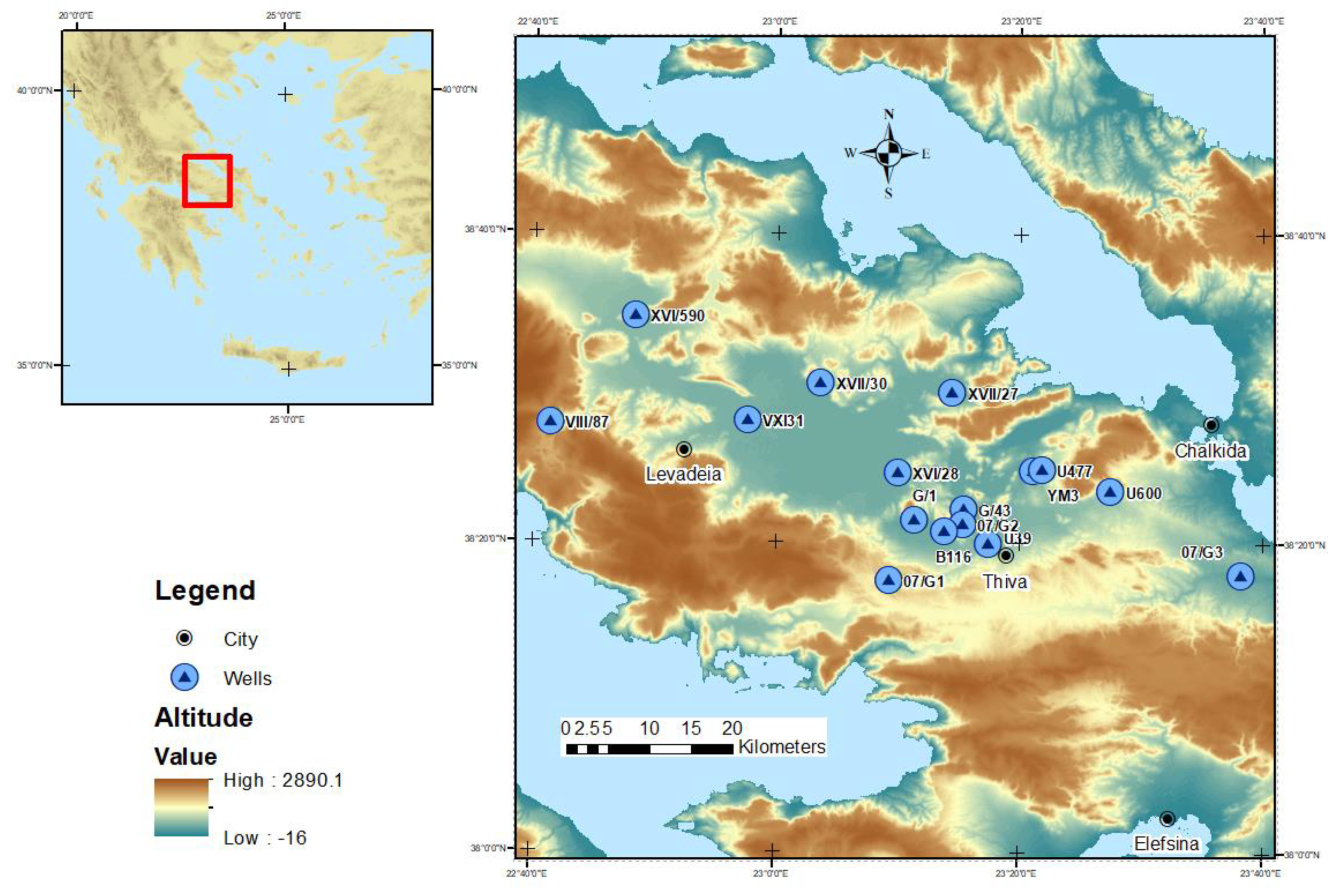
Available data on the area from the Institute of Geology and Mineral Exploration of Greece [42] include the pH, electrical conductivity, water temperature, air temperature, water level as measured from sea level, and the coordinates of each well. Other parameters that were not relevant to the current study (e.g., , , etc.) were not taken into account in this modeling approach. The available input dataset from the Institute of Geology and Mineral Exploration consisted in total of 112 records of complete data that were collected from sixteen wells. Sampling was generally performed at each well four times per year in equal intervals. The following map (Figure 1) shows the wells in the study area from which the field data measurements and concentrations were obtained.
For each well, there are numerous records of the model input variables; however, as an overview of the groundwater condition the mean values of each variable in each well are presented. The following tables (Table 1 and Table 2) list the maximum, minimum, and average concentrations and the mean values of the input parameters for each well as derived from the data analysis.
It should be noted that these wells were selected because they are in areas that have been designated as zones vulnerable to nitrate pollution and where similar climatic conditions prevail. They are not located in the same aquifer; as ANNs are data-driven models, the hydrogeological conditions did not constitute the determining factor for the selection of the wells in this study.
2. Materials and Methods
In the present study, a feed forward network was used, a type of MLP network in which the nodes are connected only in a forward way. A Bayesian Regularization (BR) algorithm was employed for the training procedure, as this is considered an appropriate training method for small input data [41]. Bayesian regularization networks are considered relatively robust, and it is difficult to overtrain or overfit them based on previous studies [40]. This eliminates the need for a separate validation dataset [43]. Nevertheless, in order to ensure the generalization ability of the network a certain percentage of the available dataset was set aside as the testing dataset. The architecture of the network was optimized by a trial-and-error procedure based on the correlation coefficient (R) between the observed data and the outputs produced by the model.
For the models that delivered satisfactory results, additional measures were estimated to further evaluate their performance. These measures were used in the statistical analysis to estimate a model’s ability to reproduce the desired values [44].
R: Pearson correlation coefficient indicates the strength of the relationship between two variables; R = ±1 denotes a perfect linear relationship between the observed () and the simulated () data, while measures in the space (−0.3, +0.3) indicate no linear relationship. Values over 0.70 signify an important correlation [45].
MAE (Mean Absolute Error): the amount of physical error in a measurement.
RMSE (Root Mean Square Error): a widely used measure of the difference between the values produced by a model and those observed (residuals).
Bias: the difference between the simulated and observed values; it can be positive or negative, and thus it provides information about the model’s tendency to overestimate or underestimate the observed data.
MAE and RMSE take values in the space (0, +∞), while Bias takes values in the space (−∞, +∞) expressed in the units of the variable being studied, with an optimal value of zero.
NSE (Nash–Sutcliffe Model Efficiency) [46]: this index, widely used in hydrological modeling, is a measure of the relationship between model errors and the real value’s variability. The NSE index takes values in the (−∞, 1) range. Values close to 1 indicate high accuracy of the model, while values close to 0 indicate that the model does not produce better results than simply taking the average value of the sample. More specifically:
- NSE = 1: there is a perfect correlation between simulated and actual values.
- NSE = 0: the model has the same precision as the average value of the actual values.
- −∞ < NSE < 0: it is preferable to use the mean value of the sample rather than the model’s predictions.
Depending on the size of the samples and the model being proposed, there have been various NSE values proposed that indicate satisfactory accuracy of the model. Positive and even low values are considered acceptable, while for values 0.65 < NSE the model is considered to be of good precision [47].
For better evaluation of model performance, the measures were estimated separately for the full data set and for the data used for the validation.
2.1. First ANN
The input variables initially studied were the well water pH, electrical conductivity, water temperature, air temperature, hydraulic head, and coordinates of the well. In this way, the model used parameters considered to affect to varying degrees the levels of nitrate pollution. The set of parameters was selected such that all could be easily measured on site, as there was no detailed information on parameters that had been used in the past in similar studies [48], for example N surplus on agricultural land, and this model was focused on using only observed data and not on modelled or mean data for the area. The lack of a large number of datasets led to the decision to use a model which could take advantage of the full dataset instead of splitting it by single wells.
The introduction of coordinates was initially inspired by geostatistical models, which have the ability to describe the spatial distribution of parameters, thereby expanding point measurements to two dimensions. [49,50]. By introducing the coordinates of each drilling well it is possible to incorporate information about their fixed characteristics, which are difficult to determine, as ANNs present the ability to derive meaning from complicated data and are capable of identifying hidden patterns and trends [51]. Air temperature is related to climatic conditions; electrical conductivity, pH, and water temperature reflect the condition of the aquifer, which affects the processes of nitrogen conversion in its different forms. Finally, the water level of the aquifer is related to seasonal conditions and the transport process of .
For all input variables, the Pearson correlation coefficient was calculated (Table 3) in relation to the concentration of nitrates. The correlation between the input and the output variables should not be very high [13], as the network tends to give weight to parameters with high correlation and underestimate the others.
No linear relationship was observed between the input variables and nitrate concentrations, suggesting that the relationships governing the physical system are very complex. Because of these low correlations, the network was driven to capture deeper relationships between the variables, thus better approaching the problem being studied. For this reason, the model was expected to lead to a smaller deviation between the observed and simulated values [13]. The results in Table 3 show that nitrate concentration has a positive correlation with electrical conductivity, water temperature, air temperature, and water level. This can be explained by nitrate ions increasing electrical conductivity; a high-water level and temperature would help the nitrates to leach and to reach the water table faster. Nitrates are known to have the exact opposite relationship with pH; higher nitrate concentrations lower pH [52].
After the trial-and-error procedure, the best architecture appeared to be that of one hidden layer with ten nodes and a sigmoid function in the first layer and linear function in the output layer as activation functions. The algorithm randomly divided the dataset such that 80% of the data were used in the training process to capture the relationship between inputs and outputs, while the remaining 20% was retained for the testing process where the performance of the trained network was evaluated in order to assess the generalization ability of the network. For replication purposes, we saved the initial random division of the dataset.
2.2. Second ANN
As mentioned above, the objective of this paper is to develop a model that has a physical meaning, i.e., where the input and output parameters are related through known environmental processes. Therefore, it was decided to examine the use of additional data in the form of a parameter that is probably linked with the level of nitrate pollution in an aquifer and in a way reflects the amount of nitrogen available for leaching into the aquifer. Hence, land use was used as an input parameter to check whether the inclusion of such information would lead to better results.
A method to quantify the land use parameter was necessary before it could be included in the list of input parameters. The coverage rate, i.e., the percentage of land area, of the different land uses within a radius of 1000 m around each drilling well were chosen for inclusion in the model. Land use information was obtained from the Corine Land Cover 2006 database (CLC2006). The Corine system provides maps of different types of land cover divided into 44 categories. For the purpose of this study, the cover map for 2006 was introduced into ArcGis 10.5 software, where the coverage rates for each well were calculated for each category. The land uses identified in the radius of 1000 m belong to nine categories:
- Discontinuous urban fabric
- Industrial or commercial units
- Road and rail networks
- Mineral extraction sites
- Non-irrigated arable land
- Permanently irrigated land
- Complex cultivation patterns
- Natural grasslands
- Sclerophyllous vegetation
The network architecture remained the same except for the number of neurons in the hidden layer, which increased as the number of input variables was now sixteen. In most cases, it is not advisable to have a small number of hidden-level neurons because the network will not be able to describe the complexity of the system being studied, leading to underfitting [53]. The optimal number of nodes after the trial-and-error procedure was set at eighteen. The architecture of the networks is illustrated below in Figure 2.
3. Results and Discussion
Our decision to include two types of input parameters in the data-driven models proved to be a correct one. The first group of input parameters constantly change over time. These include pH, electrical conductivity, water level, air temperature, and water temperature. These input parameters provide the necessary information for the model to simulate why a value at a certain point would be different over time. The second group of input parameters remains constant over time. It includes parameters that help the model to simulate the constant effects of processes that affect nitrate fluctuation and ones that differ spatially. For example, when one well is around agricultural land, it is expected to have a higher concentration of nitrates than another which is around forest land. Due to the spatial continuity of nitrate concentrations, if a well is near another well with a high concentration, it can be expected to have a higher concentration than one that is far away from all other high-concentration wells. This group includes the coordinates, and in the second ANN it includes percentages of land use classes in a buffer area around the well. All the parameters remain linked to the output parameter due to universal processes not specific for a particular site. For this reason, a model with the same parameters could be trained with data from different locations and be expected have similarly good prediction.
For future work, inclusion of subsurface material information, which unfortunately was not available for the current study area, could improve ANN results.
While it is highly improbable that all of the input parameters (pH, electrical conductivity, water level, water temperature, and air temperature) had the exact same values and the output was different, this is not impossible. This situation did not exist in our observed dataset; in case it did, a possible solution would have been to explore the possibility of using ensembles of neural networks [54,55,56] to ensure that instead of one deterministic value the output will be a range of possible values. In this way, the output parameter could have different values even for identical sets of input parameters.
Throughout the presentation of the results, we draw a distinction between training data (data used to train the ANN with the BR algorithm), test data (data never used during the training process), and the full available dataset, denoted as ‘all’. The test dataset was selected randomly from the full available dataset. However, it contains well locations that were not included in the training dataset. This fact justified our choice to include the coordinates as model inputs, providing the model with increased ability to simulate the spatial variability of nitrate concentrations in the region.
The first ANN results were satisfactory, with all the calculated model performance indices above acceptable levels according to previously published research [44,47]. However, the simulation using the second ANN yielded even better results, confirming the initial hypothesis that the ANN which included the land use input parameters would have a better ability to simulate the relevant natural processes.
Moreover, in both networks it was observed that in certain cases involving low concentrations (5 mg/L), the model provides small negative values. During the development of the network this phenomenon cannot be avoided. Although these values have no physical meaning, the difference from the actual values is small and the phenomenon is observed at low concentrations, thus it was not considered to be a problem. For this reason, after the training procedure the code was modified to replace the negative values with a value of zero. This problem can be alternatively solved using the Rectified Linear Unit (ReLU) as an activation function; however, that option was not available in our software release.
3.1. First ANN
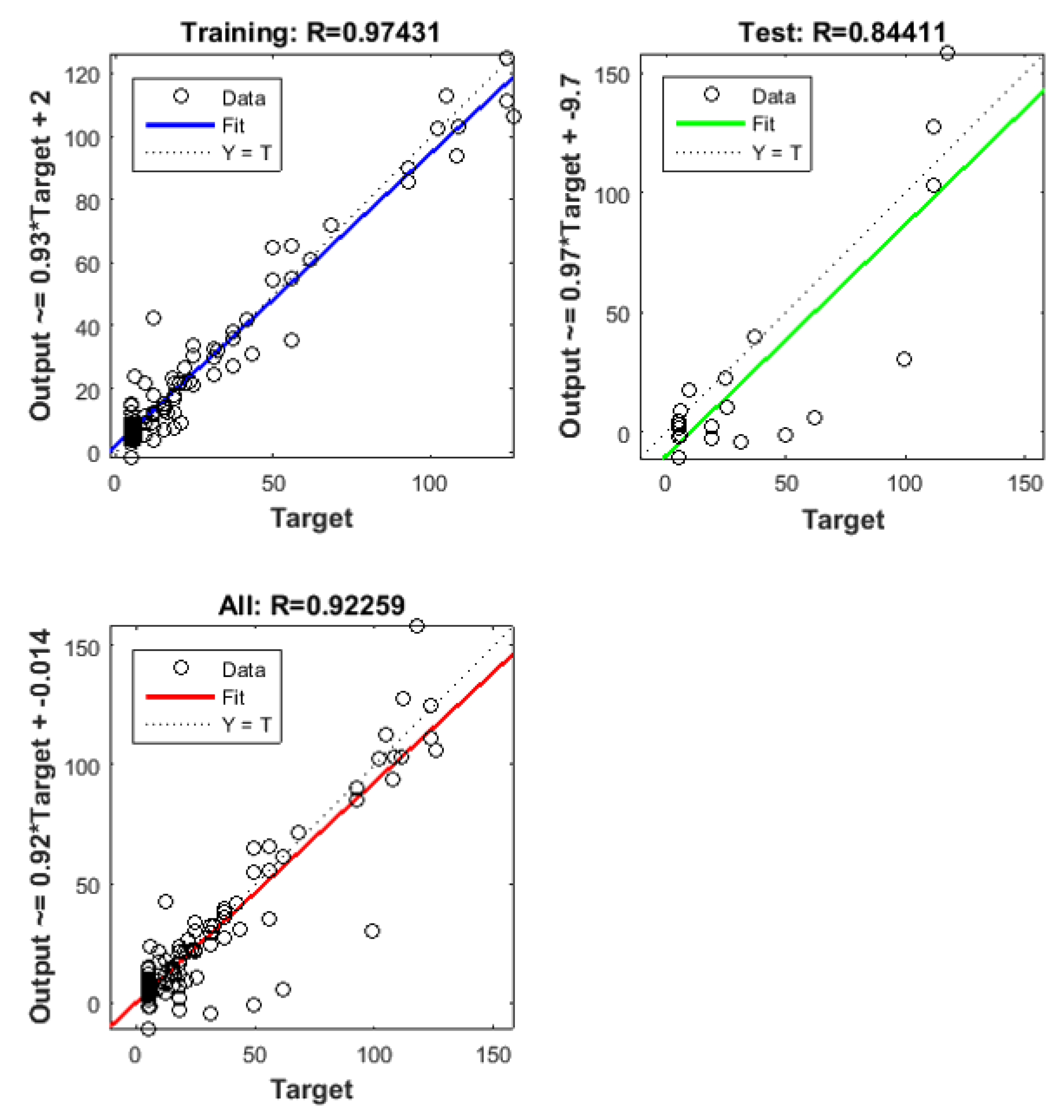
The first ANN run with the full dataset of available data was split in the way described in the Methodology section. Figure 4 shows the simulation results in scatterplots of the values in mg/L calculated by the model (Y axis) vs. the observed data (X axis target). The Pearson coefficients (R index) for the training data (top left), the verification set (top right), and the full data set (bottom left) are included above each chart. It is evident that the ANN achieved good simulation of the natural processes. Between the simulated and actual values the correlation is high in both the training set (R = 0.97) and the test set (R = 0.84), with a total correlation index of 0.92 (Figure 3). The results of both the training and the test datasets signify satisfactory performance of the model, particularly considering the small size of the available dataset.
Table 4 shows the calculated indices for the evaluation of the first ANN model’s goodness of fit.
For the full data set, the NSE is equal to 0.84, while for the test set, . As shown by the indices, the model produced satisfactory results. According to previous studies [57], RMSE and MAE values less than half the standard deviation of the observed data are considered low, showing the good performance of the model. Therefore, taking into account the RMSE and MAE indexes for the full dataset, the model has a good performance. For the test data set, however, the RMSE value is relatively high ( > 39.65/2). Furthermore, according to the Bias index the model tends to underestimate the observed values. This holds true for both the full and the test datasets, although in the full dataset it is quite low (around −2 mg/L) considering the range of the full dataset values (5–126 mg/L) and their standard deviation.
3.2. Second ANN
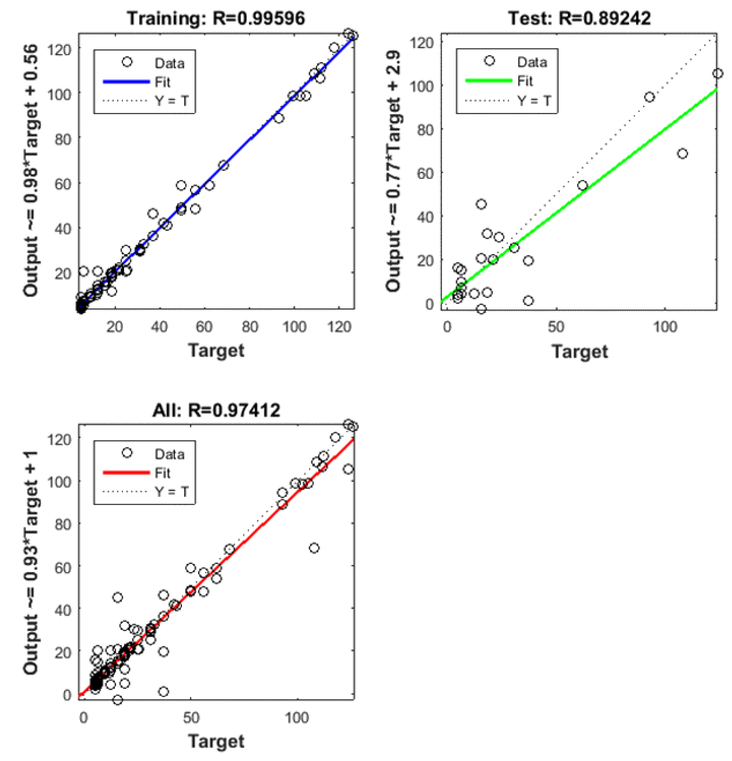
The performance of the second ANN model (Figure 4) appears to be remarkably better compared to that of the first ANN, with the correlation index of the full dataset showing R = 0.97. In the training data set the coefficient is very high (R = 1.00) and in the test set it is almost 0.05 higher than the first ANN (R = 0.89) (Figure 4).
For the full dataset, the NSE is 0.95, which is very close to the optimal value (NSE = 1), while for the test dataset it reached a value of 0.70, showing a significant increase over the first ANN where it was 0.54, an almost 30% increase in the NSE of the test data. According to all the indices, the performance of the model increased significantly when the land use parameters were added. The small difference between RMSE and MAE (15.95 mg/L–11.53 mg/L) (Table 5) indicates the absence of extreme errors, while both error indices decreased by about 30% compared to the first model. In addition, both standard deviations are less than half that of the sample, which classifies the errors as within acceptable limits. This is especially important for the test dataset, which shows the generalization ability of the model, which had an RMSE value of 15.95, far lower than the 19.82 limit. Finally, according to the Bias index it can be observed that this model tends to slightly underestimate the real values, although to a far lesser extent compared to the first model, as the value decreased by 60%.
As the inclusion of land use data improved the model results, further checks were performed to examine whether the results would further improve by increasing or decreasing the radius around the wells for which land use percentages were calculated. Adding land uses for either 500 m or 2000 m around the wells decreased the model performance, and thus the initial 1000 m radius was considered optimal.
4. Conclusions
In the present paper, the possibility of using ANNs for the estimation of concentrations in groundwater based on simple field measurements and physicochemical parameters was examined. The results of the simulations demonstrate the capability of ANNs to assess groundwater nitrate pollution when the appropriate input parameters and the optimal structure of the ANN are identified. The developed model is expected to work for any different dataset in the same region. It would require retraining with observed data if there were a willingness to apply it in a different area.
Regarding the performance of the models, the first important remark is that satisfactory network training together with good generalization capability were achieved despite the small size of the concentration data.
The first neural network, which used field data as its input parameters, achieved a satisfactory simulation. The second neural network, in which land uses in a 1000 m radius around each well were introduced as input parameters, showed increased efficiency. It is worth noting that the values of all indices improved significantly in the second model. The NSE value for the test set, the data set not used in the training process, is considered quite high (). The model’s performance is expected to increase further with newer field data and subsequent retraining of the network.
The results of the second model show that the ANN is able to simulate to a great extent the complex transport system in the geoenvironment. This is particularly important when taking into account that the estimation of concentrations is not simply based on a high correlation of variables without causality and is based rather on the factors that actually affect nitrate transport in the groundwater.
The performance that the models achieved suggests that they represent a viable solution and tool for predicting levels of pollution based on location, land use, and meteorological and hydrogeochemical data, which could form the basis for the development of.
Author Contributions
Conceptualization, I.T. and C.S.; methodology, I.T.; software, C.S.; validation, C.S. and I.T.; formal analysis, C.S.; data curation, C.S. and I.T.; writing—original draft preparation, C.S.; writing—review and editing, C.S., I.T. and G.P.K.; visualization, C.S.; supervision, G.P.K. All authors have read and agreed to the published version of the manuscript.
Funding
This research received no external funding.
Institutional Review Board Statement
Not applicable.
Informed Consent Statement
Not applicable.
Data Availability Statement
The data was available on the request of the corresponding author.
Conflicts of Interest
The authors declare no conflict of interest.
References
- Shukla, S.; Saxena, A. Global Status of Nitrate Contamination in Groundwater: Its Occurrence, Health Impacts, and Mitigation Measures. In Handbook of Environmental Materials Management; Hussain, C.M., Ed.; Springer International Publishing: Cham, Switzerland, 2018; pp. 1–21. ISBN 978-3-319-58538-3. [Google Scholar]
- Rivett, M.O.; Buss, S.R.; Morgan, P.; Smith, J.W.N.; Bemment, C.D. Nitrate Attenuation in Groundwater: A Review of Biogeochemical Controlling Processes. Water Res. 2008, 42, 4215–4232. [Google Scholar] [CrossRef] [PubMed]
- Gutiérrez, M.; Biagioni, R.N.; Alarcón-Herrera, M.T.; Rivas-Lucero, B.A. An Overview of Nitrate Sources and Operating Processes in Arid and Semiarid Aquifer Systems. Sci. Total Environ. 2018, 624, 1513–1522. [Google Scholar] [CrossRef] [PubMed]
- World Health Organization. Guidelines for Drinking—Water Quality, 4th ed.; World Health Organization: Geneva, Switzerland, 2011; ISBN 978-92-4-154815-1. [Google Scholar]
- ASCE Task Committee on Application of Artificial Neural Networks in Hydrology Artificial Neural Networks in Hydrology. I: Preliminary Concepts. J. Hydrol. Eng. 2000, 5, 115–123. [Google Scholar] [CrossRef]
- Trichakis, I.C.; Nikolos, I.K.; Karatzas, G. Artificial Neural Network (ANN) Based Modeling for Karstic Groundwater Level Simulation. Water Resour. Manag. 2011, 25, 1143–1152. [Google Scholar] [CrossRef]
- Ghose, D.; Das, U.; Roy, P. Modeling Response of Runoff and Evapotranspiration for Predicting Water Table Depth in Arid Region Using Dynamic Recurrent Neural Network. Groundw. Sustain. Dev. 2018, 6, 263–269. [Google Scholar] [CrossRef]
- ASCE Task Committee on Application of Artificial Neural Networks in Hydrology Artificial Neural Networks in Hydrology. II: Hydrologic Applications. J. Hydrol. Eng. 2000, 5, 124–137. [Google Scholar] [CrossRef]
- Lin, G.-F.; Chen, G.-R. An Improved Neural Network Approach to the Determination of Aquifer Parameters. J. Hydrol. 2006, 316, 281–289. [Google Scholar] [CrossRef]
- Nayak, P.C.; Rao, Y.R.S.; Sudheer, K.P. Groundwater Level Forecasting in a Shallow Aquifer Using Artificial Neural Network Approach. Water Resour. Manag. 2006, 20, 77–90. [Google Scholar] [CrossRef]
- Tapoglou, E.; Trichakis, I.C.; Dokou, Z.; Nikolos, I.K.; Karatzas, G.P. Groundwater-Level Forecasting under Climate Change Scenarios Using an Artificial Neural Network Trained with Particle Swarm Optimization. Hydrol. Sci. J. 2014, 59, 1225–1239. [Google Scholar] [CrossRef] [Green Version]
- Wen, X.; Feng, Q.; Deo, R.C.; Wu, M.; Si, J. Wavelet Analysis–Artificial Neural Network Conjunction Models for Multi-Scale Monthly Groundwater Level Predicting in an Arid Inland River Basin, Northwestern China. Hydrol. Res. 2017, 48, 1710–1729. [Google Scholar] [CrossRef]
- Trichakis, I.C.; Nikolos, I.K.; Karatzas, G.P. Optimal Selection of Artificial Neural Network Parameters for the Prediction of a Karstic Aquifer’s Response. Hydrol. Process. 2009, 23, 2956–2969. [Google Scholar] [CrossRef]
- El Tabach, E.; Lancelot, L.; Shahrour, I.; Najjar, Y. Use of Artificial Neural Network Simulation Metamodelling to Assess Groundwater Contamination in a Road Project. Math. Comput. Model. 2007, 45, 766–776. [Google Scholar] [CrossRef]
- Cho, K.H.; Sthiannopkao, S.; Pachepsky, Y.A.; Kim, K.-W.; Kim, J.H. Prediction of Contamination Potential of Groundwater Arsenic in Cambodia, Laos, and Thailand Using Artificial Neural Network. Water Res. 2011, 45, 5535–5544. [Google Scholar] [CrossRef] [PubMed]
- Yang, Q.; Zhang, J.; Hou, Z.; Lei, X.; Tai, W.; Chen, W.; Chen, T. Shallow Groundwater Quality Assessment: Use of the Improved Nemerow Pollution Index, Wavelet Transform and Neural Networks. J. Hydroinformatics 2017, 19, 784–794. [Google Scholar] [CrossRef]
- Stamenković, L.J. Application of ANN and SVM for Prediction Nutrients in Rivers. J. Environ. Sci. Health Part A 2021, 56, 867–873. [Google Scholar] [CrossRef] [PubMed]
- Stamenković, L.J.; Mrazovac Kurilić, S.; Presburger Ulniković, V. Prediction of Nitrate Concentration in Danube River Water by Using Artificial Neural Networks. Water Supply 2020, 20, 2119–2132. [Google Scholar] [CrossRef]
- Rohman, F.; Setiawan, D.; Prasetyatama, Y.D.; Sutiarso, L. Development of Artificial Neural Network Model for Soil Nitrate Prediction. IOP Conf. Ser. Earth Environ. Sci. 2021, 757, 012032. [Google Scholar] [CrossRef]
- Hrnjica, B.; Mehr, A.D.; Jakupovic, E.; Crnkic, A.; Hasanagic, R. Application of Deep Learning Neural Networks for Nitrate Prediction in the Klokot River, Bosnia and Herzegovina. In Proceedings of the 2021 7th International Conference on Control, Instrumentation and Automation (ICCIA), Tabriz, Iran, 23–24 February 2021; IEEE: Tabriz, Iran, 2021; pp. 1–6. [Google Scholar]
- Jung, K.; Bae, D.-H.; Um, M.-J.; Kim, S.; Jeon, S.; Park, D. Evaluation of Nitrate Load Estimations Using Neural Networks and Canonical Correlation Analysis with K-Fold Cross-Validation. Sustainability 2020, 12, 400. [Google Scholar] [CrossRef] [Green Version]
- Band, S.S.; Janizadeh, S.; Pal, S.C.; Chowdhuri, I.; Siabi, Z.; Norouzi, A.; Melesse, A.M.; Shokri, M.; Mosavi, A. Comparative Analysis of Artificial Intelligence Models for Accurate Estimation of Groundwater Nitrate Concentration. Sensors 2020, 20, 5763. [Google Scholar] [CrossRef]
- Wagh, V.; Panaskar, D.; Muley, A.; Mukate, S.; Gaikwad, S. Neural Network Modelling for Nitrate Concentration in Groundwater of Kadava River Basin, Nashik, Maharashtra, India. Groundw. Sustain. Dev. 2018, 7, 436–445. [Google Scholar] [CrossRef]
- Ostad-Ali-Askari, K.; Shayannejad, M.; Ghorbanizadeh-Kharazi, H. Artificial Neural Network for Modeling Nitrate Pollution of Groundwater in Marginal Area of Zayandeh-Rood River, Isfahan, Iran. KSCE J. Civ. Eng. 2017, 21, 134–140. [Google Scholar] [CrossRef]
- Yesilnacar, M.I.; Sahinkaya, E.; Naz, M.; Ozkaya, B. Neural Network Prediction of Nitrate in Groundwater of Harran Plain, Turkey. Environ. Geol. 2008, 56, 19–25. [Google Scholar] [CrossRef]
- Benzer, S.; Benzer, R. Modelling Nitrate Prediction of Groundwater and Surface Water Using Artificial Neural Networks. J. Polytech. 2018, 21, 321–325. [Google Scholar] [CrossRef] [Green Version]
- Huang, J.; Xu, J.; Liu, X.; Liu, J.; Wang, L. Spatial Distribution Pattern Analysis of Groundwater Nitrate Nitrogen Pollution in Shandong Intensive Farming Regions of China Using Neural Network Method. Math. Comput. Model. 2011, 54, 995–1004. [Google Scholar] [CrossRef]
- Bui, D.T.; Khosravi, K.; Karimi, M.; Busico, G.; Khozani, Z.S.; Nguyen, H.; Mastrocicco, M.; Tedesco, D.; Cuoco, E.; Kazakis, N. Enhancing Nitrate and Strontium Concentration Prediction in Groundwater by Using New Data Mining Algorithm. Sci. Total Environ. 2020, 715, 136836. [Google Scholar] [CrossRef] [PubMed]
- Elzain, H.E.; Chung, S.Y.; Senapathi, V.; Sekar, S.; Lee, S.Y.; Roy, P.D.; Hassan, A.; Sabarathinam, C. Comparative Study of Machine Learning Models for Evaluating Groundwater Vulnerability to Nitrate Contamination. Ecotoxicol. Environ. Saf. 2022, 229, 113061. [Google Scholar] [CrossRef]
- Almasri, M.N.; Kaluarachchi, J.J. Modeling Nitrate Contamination of Groundwater in Agricultural Watersheds. J. Hydrol. 2007, 343, 211–229. [Google Scholar] [CrossRef]
- Zhang, Q.; Qian, H.; Xu, P.; Li, W.; Feng, W.; Liu, R. Effect of Hydrogeological Conditions on Groundwater Nitrate Pollution and Human Health Risk Assessment of Nitrate in Jiaokou Irrigation District. J. Clean. Prod. 2021, 298, 126783. [Google Scholar] [CrossRef]
- Lehmann, J.; Schroth, G. Nutrient Leaching. In Trees, Crops, and Soil Fertility: Concepts and Research Methods; Schroth, G., Sinclair, F.L., Eds.; CABI Publishing: Cambridge, MA, USA, 2003; pp. 151–166. ISBN 978-0-85199-593-4. [Google Scholar]
- McLay, C.D.A.; Dragten, R.; Sparling, G.; Selvarajah, N. Predicting Groundwater Nitrate Concentrations in a Region of Mixed Agricultural Land Use: A Comparison of Three Approaches. Environ. Pollut. 2001, 115, 191–204. [Google Scholar] [CrossRef]
- Haynes, R.J.; Sherlock, R.R. Chapter 5—Gaseous Losses of Nitrogen. In Mineral Nitrogen in the Plant–Soil System; Haynes, R.J., Ed.; Academic Press: Cambridge, MA, USA, 1986; pp. 242–302. ISBN 978-0-12-334910-1. [Google Scholar]
- Francis, A.J.; Slater, J.M.; Dodge, C.J. Denitrification in Deep Subsurface Sediments. Geomicrobiol. J. 1989, 7, 103–116. [Google Scholar] [CrossRef]
- Morris, J.T.; Whiting, G.J.; Chapelle, F.H. Potential Denitrification Rates in Deep Sediments from the Southeastern Coastal Plain. Environ. Sci. Technol. 1988, 22, 832–836. [Google Scholar] [CrossRef] [PubMed]
- Nielsen, M.E.; Fisk, M.R.; Istok, J.D.; Pedersen, K. Microbial Nitrate Respiration of Lactate at in Situ Conditions in Ground Water from a Granitic Aquifer Situated 450 m Underground. Geobiology 2006, 4, 43–52. [Google Scholar] [CrossRef]
- Di, H.J.; Cameron, K.C.; Moore, S.; Smith, N.P. Contributions to Nitrogen Leaching and Pasture Uptake by Autumn-Applied Dairy Effluent and Ammonium Fertilizer Labeled with 15N Isotope. Plant Soil 1999, 210, 189–198. [Google Scholar] [CrossRef]
- Cameron, K.C.; Di, H.J.; Moir, J.L. Nitrogen Losses from the Soil/Plant System: A Review: Nitrogen Losses. Ann. Appl. Biol. 2013, 162, 145–173. [Google Scholar] [CrossRef]
- Burden, F.; Winkler, D. Bayesian Regularization of Neural Networks. In Artificial Neural Networks; Livingstone, D.J., Ed.; Methods in Molecular BiologyTM; Humana Press: Totowa, NJ, USA, 2008; Volume 458, pp. 23–42. ISBN 978-1-58829-718-1. [Google Scholar]
- Okut, H. Bayesian Regularized Neural Networks for Small n Big p Data. In Artificial Neural Networks—Models and Applications; Rosa, J.L.G., Ed.; InTech: Sao Paulo, Brazil, 2016; ISBN 978-953-51-2704-8. [Google Scholar]
- Giannoulopoulos, P. Identificative Hydrogeological—Hydrochemical Survey of Quality Charge of Groundwater of the Wider Area of the Basin of Asopos, Boeotia; Institute of Geology and Mineral Exploration, Directorate of Hydrogeology: Athens, Greece, 2008. (In Greek) [Google Scholar]
- Kayri, M. Predictive Abilities of Bayesian Regularization and Levenberg–Marquardt Algorithms in Artificial Neural Networks: A Comparative Empirical Study on Social Data. Math. Comput. Appl. 2016, 21, 20. [Google Scholar] [CrossRef]
- Matiatos, I.; Varouchakis, E.; Papadopoulou, M. Statistical Sensitivity Analysis of Multiple Groundwater Mass Transport Models. In Proceedings of the 10th International Hydrogeological Congress of Greece, Thessaloniki, Greece, 8–10 October 2014; pp. 447–456. [Google Scholar]
- Tichý, M. Applied Methods of Structural Reliability; Topics in Safety, Reliability and Quality; Springer Netherlands: Dordrecht, The Netherlands, 1993; Volume 2, ISBN 978-94-010-4861-3. [Google Scholar]
- Nash, J.E.; Sutcliffe, J.V. River Flow Forecasting through Conceptual Models Part I—A Discussion of Principles. J. Hydrol. 1970, 10, 282–290. [Google Scholar] [CrossRef]
- Moriasi, D.N.; Arnold, J.G.; Van Liew, M.W.; Bingner, R.L.; Harmel, R.D.; Veith, T.L. Model Evaluation Guidelines for Systematic Quantification of Accuracy in Watershed Simulations. Trans. ASABE 2007, 50, 885–900. [Google Scholar] [CrossRef]
- Knoll, L.; Breuer, L.; Bach, M. Large Scale Prediction of Groundwater Nitrate Concentrations from Spatial Data Using Machine Learning. Sci. Total Environ. 2019, 668, 1317–1327. [Google Scholar] [CrossRef]
- Varouchakis, Ε.A.; Hristopulos, D.T. Comparison of Stochastic and Deterministic Methods for Mapping Groundwater Level Spatial Variability in Sparsely Monitored Basins. Environ. Monit. Assess. 2013, 185, 1–19. [Google Scholar] [CrossRef]
- Tapoglou, E.; Karatzas, G.P.; Trichakis, I.C.; Varouchakis, E.A. Temporal and Spatial Prediction of Groundwater Levels Using Artificial Neural Networks, Fuzzy Logic and Kriging Interpolation. In Proceedings of the EGU General Assembly Conference Abstracts, Vienna, Austria, 2 May–27 April 2014; Volume 16. [Google Scholar]
- Haykin, S.S. Neural Networks: A Comprehensive Foundation; Prentice Hall: Upper Saddle River, NJ, USA, 1999; ISBN 978-0-13-273350-2. [Google Scholar]
- Glass, C.; Silverstein, J. Denitrification Kinetics of High Nitrate Concentration Water: PH Effect on Inhibition and Nitrite Accumulation. Water Res. 1998, 32, 831–839. [Google Scholar] [CrossRef]
- Panchal, F.S.; Panchal, M. Review on Methods of Selecting Number of Hidden Nodes in Artificial Neural Network. Int. J. Comput. Sci. Mob. Comput. 2014, 3, 455–464. [Google Scholar]
- Nagahamulla, H.R.K.; Ratnayake, U.R.; Ratnaweera, A. An Ensemble of Artificial Neural Networks in Rainfall Forecasting. In Proceedings of the International Conference on Advances in ICT for Emerging Regions (ICTer2012), Colombo, Sri Lanka, 12–15 December 2012; pp. 176–181. [Google Scholar]
- Yao, X.; Islam, M.M. Evolving Artificial Neural Network Ensembles. IEEE Comput. Intell. Mag. 2008, 3, 31–42. [Google Scholar] [CrossRef]
- Nourani, V.; Gökçekuş, H.; Gichamo, T. Ensemble Data-Driven Rainfall-Runoff Modeling Using Multi-Source Satellite and Gauge Rainfall Data Input Fusion. Earth Sci. Inform. 2021, 14, 1787–1808. [Google Scholar] [CrossRef]
- Singh, J.; Knapp, H.V.; Arnold, J.G.; Demissie, M. Hydrological Modeling of the Iroquois River Watershed Using Hspf and Swat. JAWRA J. Am. Water Resour. Assoc. 2005, 41, 343–360. [Google Scholar] [CrossRef]
Figure 1.
The area of study in central Greece, with the topography and well locations denoted (right) and its location, shown as a red rectangle on the full map of the Balkan peninsula in Europe (left).
Figure 1.
The area of study in central Greece, with the topography and well locations denoted (right) and its location, shown as a red rectangle on the full map of the Balkan peninsula in Europe (left).

Figure 2.
Model architecture. The first ANN (left) includes pH, electrical conductivity, X, Y, water level, water temperature, and air temperature as inputs, one hidden layer, and nitrate concentration as the output. The second ANN (right) additionally includes land use percentages as inputs.
Figure 2.
Model architecture. The first ANN (left) includes pH, electrical conductivity, X, Y, water level, water temperature, and air temperature as inputs, one hidden layer, and nitrate concentration as the output. The second ANN (right) additionally includes land use percentages as inputs.

Figure 3.
Results of first ANN-R coefficient for the training (upper left), test (upper right), and full (lower left) datasets.
Figure 3.
Results of first ANN-R coefficient for the training (upper left), test (upper right), and full (lower left) datasets.

Figure 4.
Results of second ANN-R coefficient for the training (upper left), test (upper right), and full (lower left) datasets.
Figure 4.
Results of second ANN-R coefficient for the training (upper left), test (upper right), and full (lower left) datasets.


Table 1.
Minimum, maximum, and mean concentration in the study area.
| Well | Min Concentration (mg/L) | Max Concentration (mg/L) | Mean Concentration (mg/L) |
|---|---|---|---|
| G/1 | 5 | 55.8 | 23.39 |
| G/43 | 5 | 15.5 | 9.93 |
| YM3 | 5 | 49.6 | 17.68 |
| XVI/31 | 5 | 43.4 | 11.98 |
| 07/G1 | 37.2 | 124 | 88.49 |
| 07/G2 | 5 | 18.1 | 12.87 |
| 07/G3 | 5 | 99.2 | 20.56 |
| U39 | 55.8 | 126 | 89.50 |
| U477 | 37.2 | 37.2 | 37.20 |
| U600 | 41.8 | 55.8 | 48.80 |
| VIII/87 | 5 | 12.4 | 7.00 |
| XVI/28 | 5 | 62 | 24.00 |
| XVII/27 | 18.6 | 20.5 | 19.23 |
| XVII/30 | 5 | 12.4 | 6.85 |
| Β116 | 12.4 | 12.4 | 12.40 |
| XVI/590 | 18.6 | 32.6 | 26.10 |
Table 2.
Input parameter mean values.
| Mean Values | |||||
|---|---|---|---|---|---|
| Well | Water Level (m) | Electrical Conductivity (μS/cm) | Air Temperature (°C) | Water Temperature (°C) | pH |
| G/1 | 17.05 | 608.73 | 20.56 | 18.37 | 7.52 |
| G/43 | 31.10 | 489.50 | 17.75 | 18.50 | 7.41 |
| YM3 | 22.96 | 668.78 | 26.33 | 18.56 | 8.10 |
| XVI/31 | 4.64 | 592.09 | 19.20 | 17.17 | 7.80 |
| 07/G1 | 27.27 | 713.13 | 21.04 | 16.54 | 7.59 |
| 07/G2 | 35.89 | 511.00 | 24.50 | 19.67 | 7.94 |
| 07/G3 | 51.29 | 1069.00 | 21.20 | 17.35 | 7.79 |
| U39 | 28.78 | 770.00 | 24.60 | 18.68 | 7.85 |
| U477 | 65.68 | 761.00 | 30.30 | 19.40 | 7.25 |
| U600 | 164.21 | 846.00 | 26.35 | 19.45 | 7.79 |
| VIII/87 | 13.16 | 670.05 | 22.46 | 14.97 | 7.51 |
| XVI/28 | 21.64 | 770.67 | 24.97 | 18.73 | 7.52 |
| XVII/27 | 67.12 | 550.00 | 18.80 | 18.50 | 7.76 |
| XVII/30 | 8.16 | 650.50 | 21.33 | 18.08 | 7.46 |
| Β116 | 25.44 | 895.00 | 31.40 | 19.60 | 8.13 |
| XVI/590 | 8.58 | 535.00 | 23.17 | 18.03 | 7.70 |
Table 3.
Correlation coefficient of input variables with nitrate concentration.
| Input Parameter | pH | Electrical Conductivity | Water Temperature | Air Temperature | Water Level |
|---|---|---|---|---|---|
| Correlation coefficient | −0.02 | 0.18 | 0.16 | 0.08 | 0.12 |
Table 4.
First model indices.
| Index | All | Test |
|---|---|---|
| RMSE (mg/L) | 13.25 | 26.18 |
| MAE (mg/L) | 7.17 | 17.46 |
| Bias (mg/L) | −2.14 | −10.93 |
| NSE | 0.84 | 0.54 |
| St. Deviation | 33.33 | 39.65 |
Table 5.
Second model indices.
| Index | All | Test |
|---|---|---|
| RMSE (mg/L) | 7.56 | 15.95 |
| MAE (mg/L) | 3.65 | 11.53 |
| Bias (mg/L) | −0.82 | −4.20 |
| NSE | 0.95 | 0.70 |
| St. Deviation | 33.33 | 34.83 |
Publisher’s Note: MDPI stays neutral with regard to jurisdictional claims in published maps and institutional affiliations. |
© 2022 by the authors. Licensee MDPI, Basel, Switzerland. This article is an open access article distributed under the terms and conditions of the Creative Commons Attribution (CC BY) license (https://creativecommons.org/licenses/by/4.0/).
Share and Cite
MDPI and ACS Style
Stylianoudaki, C.; Trichakis, I.; Karatzas, G.P. Modeling Groundwater Nitrate Contamination Using Artificial Neural Networks. Water 2022, 14, 1173. https://doi.org/10.3390/w14071173
AMA Style
Stylianoudaki C, Trichakis I, Karatzas GP. Modeling Groundwater Nitrate Contamination Using Artificial Neural Networks. Water. 2022; 14(7):1173. https://doi.org/10.3390/w14071173
Chicago/Turabian StyleStylianoudaki, Christina, Ioannis Trichakis, and George P. Karatzas. 2022. "Modeling Groundwater Nitrate Contamination Using Artificial Neural Networks" Water 14, no. 7: 1173. https://doi.org/10.3390/w14071173
Note that from the first issue of 2016, this journal uses article numbers instead of page numbers. See further details here.