
Automated Monitoring of a High-Speed Flocculation Flat-Bottomed Sludge Blanket Clarifier Pond during Drought and Flood Conditions


1
Graduate Institute of Environmental Engineering, National Taiwan University, Taipei 10617, Taiwan
2
Tai-Yu Corporation, New Taipei 24251, Taiwan
*
Author to whom correspondence should be addressed.
Water 2022, 14(7), 1170; https://doi.org/10.3390/w14071170
Submission received: 17 March 2022
/
Revised: 1 April 2022
/
Accepted: 1 April 2022
/
Published: 6 April 2022
(This article belongs to the Section Hydrology)
Abstract
:The occasional rains that occur during dry seasons often stir up the bottom sediment of reservoirs, which leads to high turbidity and electrical conductivity in raw waters received by water utility companies. A newly developed real-time precision multi-layer sensor (RPMS) system was used to monitor a high-speed flocculation flat-bottomed sludge blanket clarifier (HFSBC) pond in real time to solve the water quality problems caused by drought and flood conditions. The RPMS is capable of monitoring the thickness of a sludge blanket; if the coagulation and sedimentation processes of the HFSBC are not working well, the sludge blanket will be thin and have a low sludge concentration. Conversely, if the HFSBC is working properly, the sludge blanket will have a thick and highly concentrated layer of sludge. Any heavy metals that are not removed by water treatment processes will enter the water supply network, which will result in poor water quality for end users. Against the backdrop of intensifying climate change, the enhancement of automated monitoring systems and adaptation processes will be an important part of efforts to minimize and resolve acute changes in water quality.
1. Introduction
Over the past few years, the global climate change has caused increasingly frequent and severe acute changes in water quality. This phenomenon has been linked to rainfall-induced perturbations in reservoirs and rivers [1,2]. Ochoa-Contreras et al. [3] also observed that the distribution of heavy metal concentrations in sedimentary rocks can be used to predict the heavy metals that have the greatest influence on water quality. To ascertain whether the raw water in a reservoir is polluted by heavy metals, the Sediment Quality Guidelines can be used to analyze sediment toxicity and pollutants in the water column [4,5]. Palma et al. [6] used land use/land cover changes to explain nutrient and organic matter concentrations in reservoirs, thereby providing guidance for water management policies to reduce surface water pollution. In many countries, large amounts of resources have been dedicated to the elimination of pollution sources. However, Česonienė et al. [7] found that the removal of pollution sources does not necessarily improve the quality of lake water because secondary pollution caused by sludge in the water can worsen the quality.
In recent years, the use of automated water quality sensors to help water resource managers to cope with acute water quality changes caused by climate change has become an important area for study. Numerous studies have been performed worldwide to improve the cost efficiency of water quality monitoring methods to provide clean and potable drinking water in a more efficient manner. Aqueous chemical detection is most commonly performed using fluorescence or optical techniques. For instance, Zhou et al. [8] used a fluorescence technique to detect dissolved organic matter in lake waters. Li et al. [9] used fluorescence spectroscopy to establish a method for tracking changes in the chemical composition of dissolved organic matter via fluorescence measurements, which can be used to predict changes in water quality and improve the safety of drinking water. Beauchamp et al. [10] used 254 nm (UV254) measurements to evaluate the optimality of alum dosage.
By combining water quality monitoring instruments with digital sampling technologies, it is possible to continuously monitor water conditions in real time. For example, Sun et al. [11] used confocal laser scanning microscopy and image analysis to monitor the biofouling of hollow fiber ultrafiltration membranes in the ozonation, biofiltration, and membrane filtration processes and to quantitatively and qualitatively analyze the biofouling process. Fortunato et al. [12] used optical coherence tomography to monitor fouling layer formation during the initial days of operation of a membrane bioreactor (MBR) and monitored the fouling of the MBR in real time under a variety of operating conditions. Kim et al. [13] used a silicon photomultiplier and Ce-doped GAG (Gd3Al2Ga3O12) scintillators to develop a miniature radiation portal monitor, which was combined with an application for PCs and mobile phones to monitor radiation in water piping. This system has good linearity with respect to radiation intensity, good channel linearity with respect to energy, and excellent energy resolution. Fujioka et al. [14] used a real-time bacteriological counter to perform online bacteria counting in the influent and effluent of a full-scale sand filter. To utilize the outstanding chemical and optical properties of carbon dots, Rao et al. [15] developed biomass-based carbon dots to develop a smartphone-based portable detection platform for the online analysis of Al3+ and H2O contents, which can be used to inspect tap water and alcoholic drinks.
In 2021, Taiwan experienced a severe drought, which caused the water storage level of the Shihmen Dam to decrease to only 205.99 m on 26 May. Because the dam is severely silted, many end users reported water quality problems such as yellow-colored tap water as the water level approached the bottom of the reservoir. The reason for these water quality problems was rainfall in the water catchment area, which perturbed the bottom sediment of the reservoir and released previously trapped heavy metals from the sediment. Consequently, the raw water drawn by the water utility company had high levels of turbidity and conductivity. Aside from the inadequacies of the treatment plant’s water clarifying capabilities, heavy metals such as Fe, Mn, and Al that were previously precipitated in the water supply network’s pipelines might have redissolved and flowed along the water supply network owing to the water having a low pH and low residual chlorine concentrations. Kurajica et al. [16] studied the factors that influence As, Al, and Mn concentrations in a drinking water supply system and found that they are affected by the pH and organic matter content. They also observed that the oxygen reduction potential has a greater impact on Mn concentration than pH and that the addition of ClO2 at a high pH oxidizes Mn and thus forms Mn particles, which combine with Al and Fe coagulants to form precipitates. Because the Mn particles may settle in the water supply network, turning on a fire hydrant may perturb the water flow and dislodge the Mn deposits, which then affect tap water quality.
It may be surmised that Taiwan will face acute water quality degradation during periods of drought. In view of the water quality issues caused by climate change, studies about water quality changes at different water depths in water clarifying ponds are scarce. In 2021, the arrival of the Meiyu front at the end of May to early June ended the 2021 drought of Taiwan but also caused the first high turbidity incidents in raw water supplies. The next high turbidity incident was caused by Typhoon In-fa, which landed on 21 July, 2021 and increased the water level in the Shihmen Dam to its maximum value.
The 2021 drought of Taiwan shed light on the difficulty of balancing water quality with water supply continuity. Diaz-Alcaide et al. [17] stated that safe water access is a manifold of concepts that include collection time, distance from households, and water quality, affordability, and reliability of water sources. Therefore, putting too much focus on water quality may reduce water output and cause water insecurity. For instance, the western half of Taiwan (from Changhua to Taoyuan) would have faced even stricter water supply restrictions if water quality was prioritized over water supply. Conversely, loosening water quality standards would have placed the safety of end-user water supplies at risk during droughts. Therefore, a water utility company can only choose between maintaining the supply of water with a lower water quality or cutting the water supplies. The balancing of these options is a problem that will require careful consideration in the near future.
In this work, we investigated the coagulation performance of a high-speed flocculation flat-bottomed sludge blanket clarifier (HFSBC). In conventional water treatment plants, the only processes that can be used to remove heavy metals ions and suspended particles from raw water are pH adjustment, pre-chlorination, and addition of coagulants and flocculants. These processes cause heavy metal ions to precipitate into fine particles and then coagulate with other suspended particles to form sludge flocs, which can be removed via settling or filtration by a rapid filtration pond. To improve the coagulation performance of HFSBCs, a real-time precision multi-layer sensor (RPMS) was used to monitor the operations of an HFSBC in real time. This system is capable of monitoring the thickness of the sludge blanket in the HFSBC; if the coagulation and flocculation processes of the HFSBC are not functioning correctly, the sludge blanket will be thin and have a low sludge concentration. Conversely, if the HFSBC is functioning correctly, the sludge blanket will be thick and highly concentrated.
2. Materials and Methods
2.1. Instrument Operating Principles
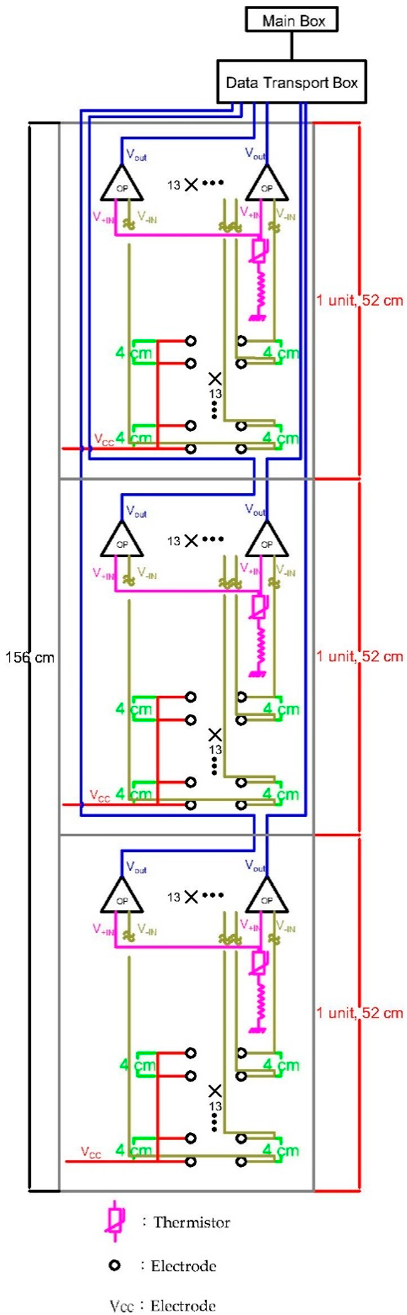
The RPMS system (Figure 1), which was developed in this work, uses conductivity meters and electrodes to measure the thickness of the sludge blanket and the electrical conductivity of the water column. The main difference between an RPMS and a conventional conductivity meter is that the latter provides well-defined measurements in absolute terms, whereas the former can only produce relative measurements. In conventional conductivity meters, a current is passed through a 1 cm2 cross section, and the measured conductivity is the reciprocal of the resistance of a 1 cm column. The unit of measurement of a conventional conductivity meter is mho/cm (mmho/cm and μmho/cm for conductivities in the range of 10−3 and 10−6, respectively). An RPMS has an electrode spacing of 4.5 cm and works like a filter with multiple sets of paralleled electrodes. The spacing between each set of electrodes is 4 cm, and the relative conductivity of the solution is inferred via comparisons with a known set of resistivity data. Unlike conventional conductivity meters, it is not yet possible to calibrate RPMS measurements to absolute conductivity values. Therefore, their conductivity measurements are expressed in units of R-EC (Relative Electrical conductivity). One RPMS is composed of 3 groups of sensing units connected in series. Every group of sensing unit has 13 pairs of electrodes. One RPMS is 156 cm long. In this study, 2 RPMS were used in series. The sensing depth of this study was 312 cm from the bottom of the pool.
2.2. Experimental Site
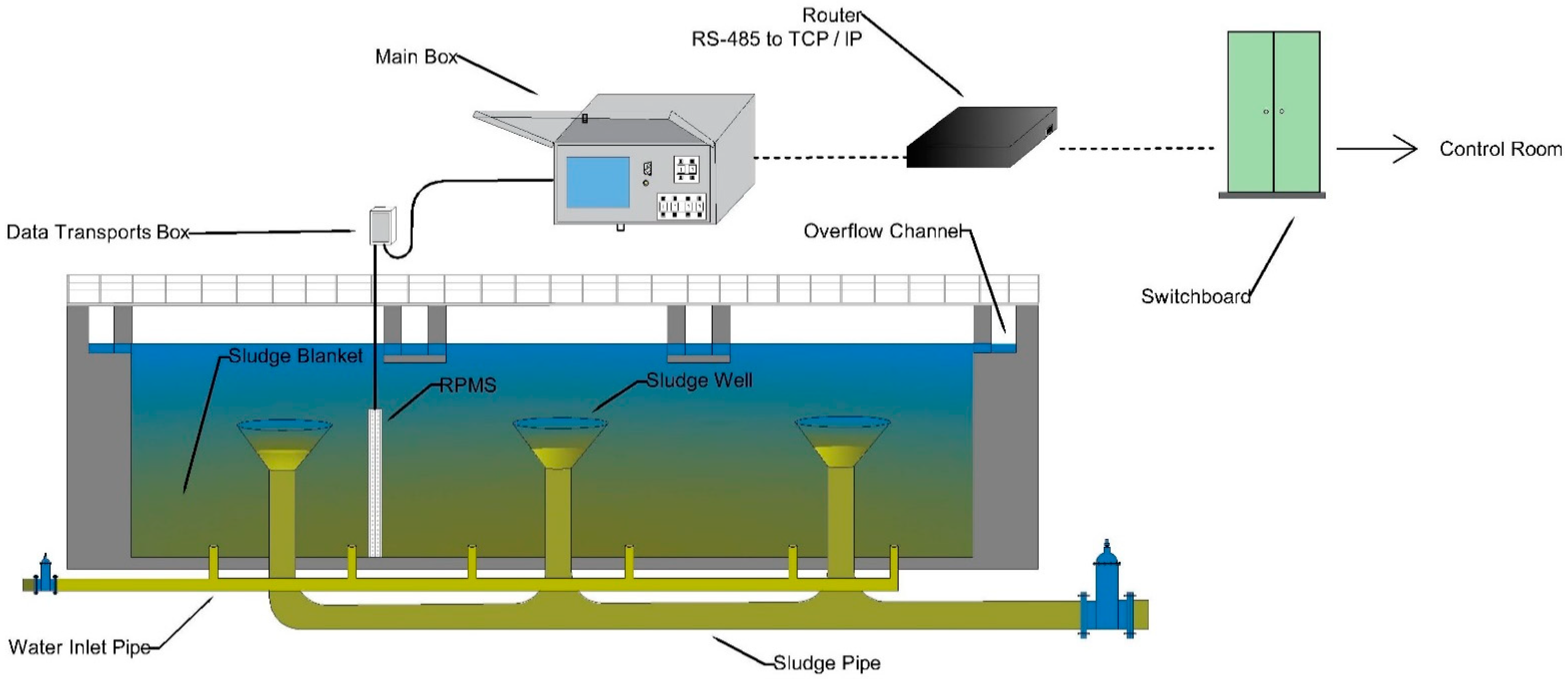
Coagulant addition is a crucial part of the water treatment process because the efficacy of this process will ultimately determine the quality of the water output from the water treatment plant. If the coagulation process is impaired, the resulting flocs may not be heavy enough to settle, which will prevent their removal from the water column via settling. The experimental site of this study was an HFSBC (Figure 2) in a water treatment plant in Taoyuan, Taiwan. The water quality of the raw waters received by this plant is strongly correlated with the weather conditions because heavy rains will cause significant increases in the turbidity (particle content) of the raw waters. Coagulant addition is the main method by which these suspended particles are removed from the water.
In this experiment, the length of the RPMS was 3 m, and the depth of the HFSBC was 5 m. The pond inlet was located at the bottom of the pond, and a sludge cone was set at a depth of 2 m to collect and discharge the sludge. Therefore, the coagulated sludge formed a sludge blanket at depths between 2 m and 5 m, which would intercept suspended solids (SS) in the water. The RPMS was installed at a depth of approximately 2 m from the bottom of the HFSBC to perform long-term monitoring of the sludge blanket’s thickness and of the changes in water quality at each depth of the pond.
2.3. Sample Acquisition
Water quality analysis was performed on water samples taken from each layer of the pond to ascertain the primary cause of their differences in electrical conductivity. To this end, 2000 mL water samples were taken inside the overflow channel (0 m) and at depths of 1.0–1.5 m (1.0 m), 2.0–2.5 m (2.0 m), 3.0–3.5 m (3.0 m), 4.0–4.5 m (4.0 m), and 4.5–5.0 m (4.5 m). The samples were acquired on 4 June 2021, 10 June 2021, 20 July 2021, and 26 July 2021.
2.4. Sample Analysis
The pH, SS, total dissolved solids (TDS), dissolved heavy metal (Fe, Al, and Mn) concentrations, and total heavy metal (Fe, Al, and Mn) concentrations of the samples were measured. The heavy metals were measured by inductively coupled plasma–optical emission spectrometry (ICP–OES) using an Agilent 700 series ICP–OES. The total heavy metal concentration was measured by first heating and digesting the sample in nitric acid and then analyzing the filtered digestion solution.
3. Results
3.1. Short-Term Monitoring
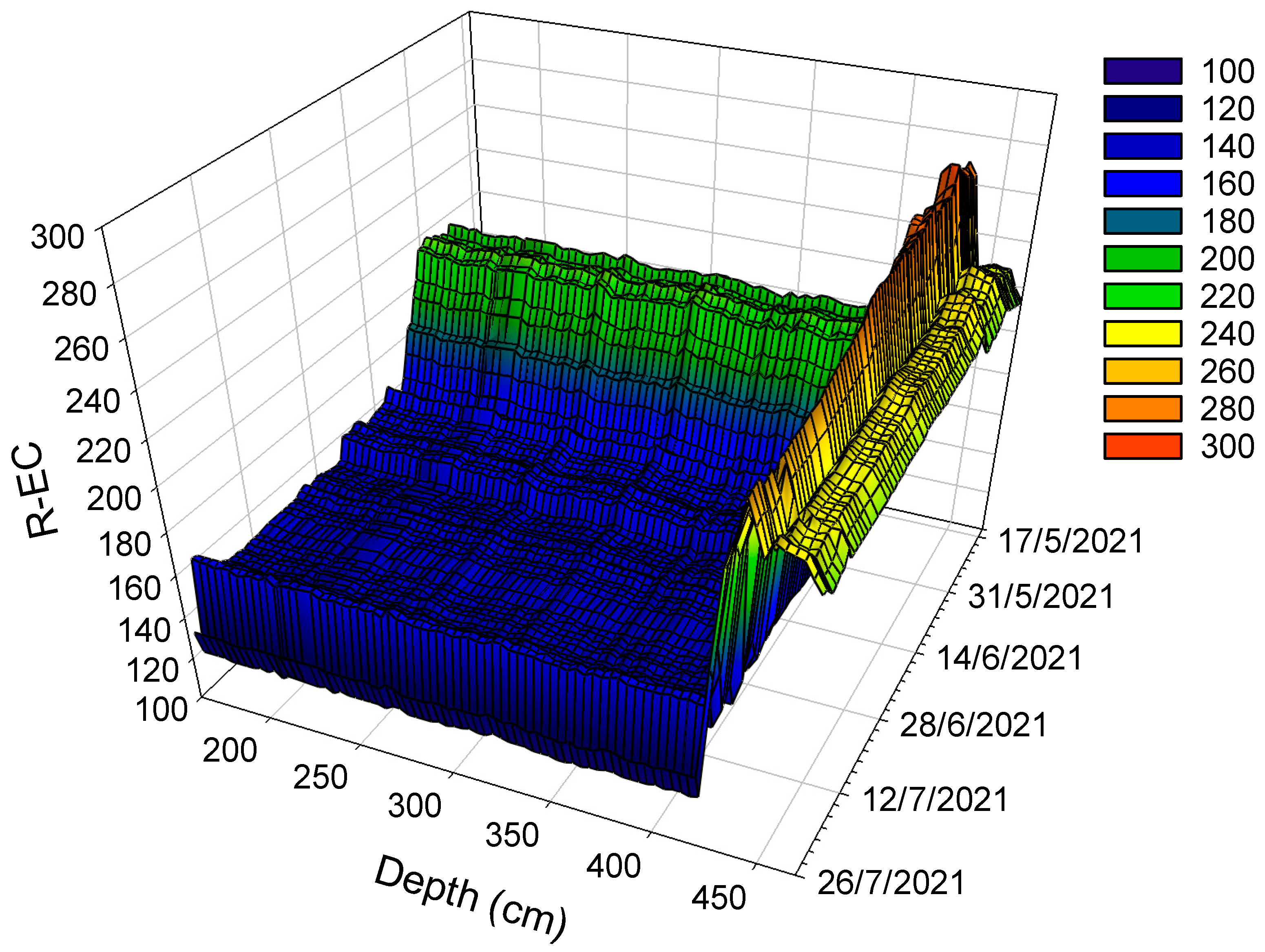
The HFSBC was monitored from 15 May 2021 to 26 July 2021. The electrical conductivities at each depth of the HFSBC during the monitoring period are shown in Figure 3.
The water conductivities at all depths gradually began to increase from 15 May onward. The presence of a significant R-EC peak between 440 cm and 416 cm implied that the sludge blanket was located at these depths. The highest measured conductivity during the monitoring period occurred at 428 cm on 24 May (279 R-EC). If it is assumed that each layer differs by a conductivity of 20 R-EC or more, the pond may be divided into three layers. From deep to shallow, the three layers are the inflow mixing layer (468–440 cm), the sludge layer (440–416 cm), and the clear-water layer (416–160 cm). From 15 May onward, the sludge layer was approximately 24 cm thick; this thickness was maintained until 16 July. The R-EC of the sludge decreased over time, and the thickness of the sludge layer decreased to 20 cm on 20 July. These changes were likely related to the changes in raw-water turbidity; because the concentration of sludge in raw water depends on its turbidity, the lower the turbidity, the lower the concentration of sludge in the sludge blanket.
The conductivity of the clear-water layer increased from 189 R-EC on 15 May to 217 R-EC on 2 June and then gradually decreased to 147 R-EC on 22 July. The conductivity of this layer spiked to 165 R-EC on 23 July and 24 July before decreasing to 130 R-EC on 25 July and 26 July. As these changes coincided with rainfall events, we investigated the relationship between rainfall and changes in electrical conductivity in greater detail.
To explain the results shown in Figure 3, the relationship between water quality and R-EC was analyzed via water samples taken at different water depths. It was assumed that the period from 4 June to 10 June corresponded to the transition from drought to end of drought, whereas the period from 20 July to 26 July corresponded to the transition from the stable pre-typhoon period to the post-typhoon period. To elucidate the cause of the changes in electrical conductivity in the clear-water layer, we measured the SS, TDS, dissolved heavy metal (Al, Mn, and Fe) concentrations, and total heavy metal (Al, Mn, and Fe) concentrations of water samples taken at depths of 0.0 (inside the overflow channel), 1.0, 2.0, 3.0, 4.0, and 4.5 m during the aforementioned periods.
3.2. Water Quality Analysis
3.2.1. Sludge and TDS
Table 1 and Table 2 show that the sludge concentration quickly decreased to 10 ppm at depths shallower than 2.0 m. This occurred because the opening of the sludge cone (used by the HFSBC to discharge sludge) was located at a depth of approximately 2.0 m. Thus, at depths less than 2.0 m, the sludge would be discharged from the pond via the sludge cone, which explains why the sludge concentrations decreased quickly after this point.
The variations of the distribution of the sludge concentration were linked to changes in the average raw-water turbidities. For instance, the 2.0–2.5 m difference between the 4-day average turbidities was equal to the multiplicative difference between the sludge concentrations at the bottom of the pond (4.5 m). Therefore, it may be inferred that the bottom sludge of the HFSBC pond was retained for an average of 4 days.
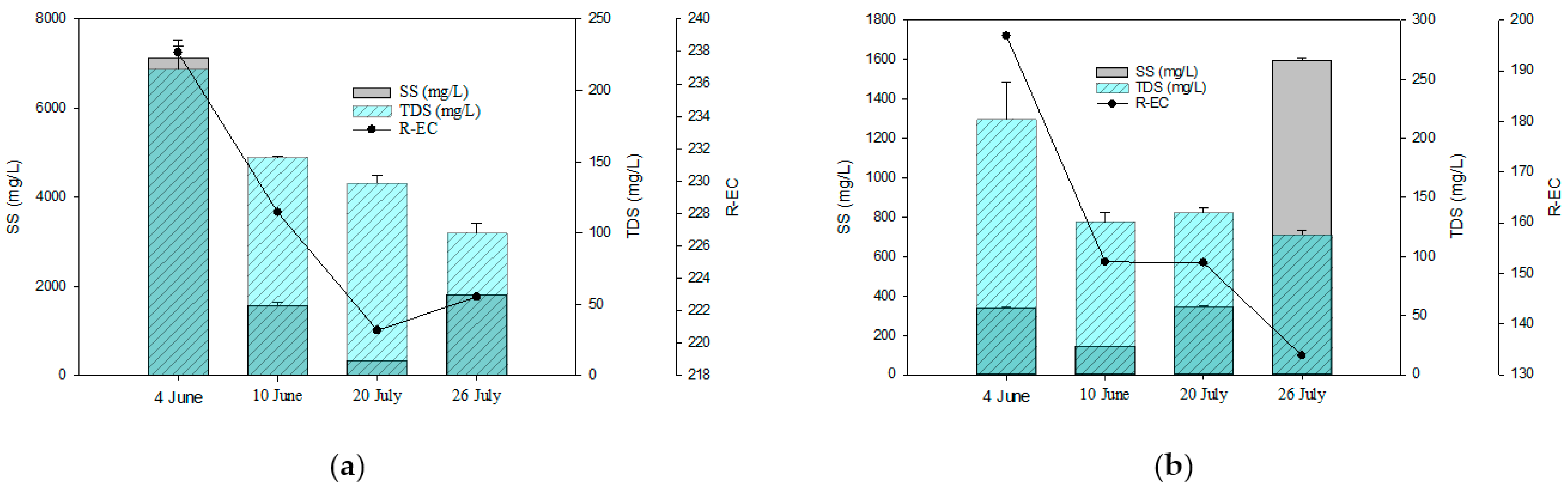
In summary, the electrical conductivity is affected by the sludge concentration and also by the TDS. Figure 4 shows that the TDS values for each day generally varied between 0.5% and 20.0% from one depth to another, whereas the SS decreased with the depth and could vary by 95% to 6% from one depth to another. This shows that depth-wise variations in SS can be much larger than those in TDS.
On 4 June, 10 June, 10 July, and 26 July, the variations in R-EC were generally less than 7.2% at 4.5 m; however, they increased to 32.4% at 2.0 m. This shows that the water quality at the bottom of the pond did not significantly affect conductivity. However, the water quality at 2.0 m, which had undergone filtering by the sludge blanket and settling, did show a significant correlation with R-EC. It is hypothesized that this correlation is caused by dissolved heavy metals in the water; the higher the concentration of dissolved heavy metals, the higher the conductivity. As the optimality of the coagulant dosage is one of the most important factors for the concentration of heavy metals in the clear-water layer, it was necessary to analyze the total heavy metal concentration and compute the difference between dissolved and total heavy metal concentrations to elucidate the distribution of heavy metals in the HFSBC pond at each time point.
Because end users reported that yellow water came out of their taps and polyaluminum chloride (PAC) was used as the coagulant in the water treatment plant, water quality analyses were performed by measuring the Al, Mn, and Fe concentrations in the water. Because a portion of the heavy metals would be adsorbed by flocs after coagulation, the total and dissolved heavy metal concentrations were both analyzed to elucidate the state of the heavy metals in the HFSBC pond.
3.2.2. Heavy Metals
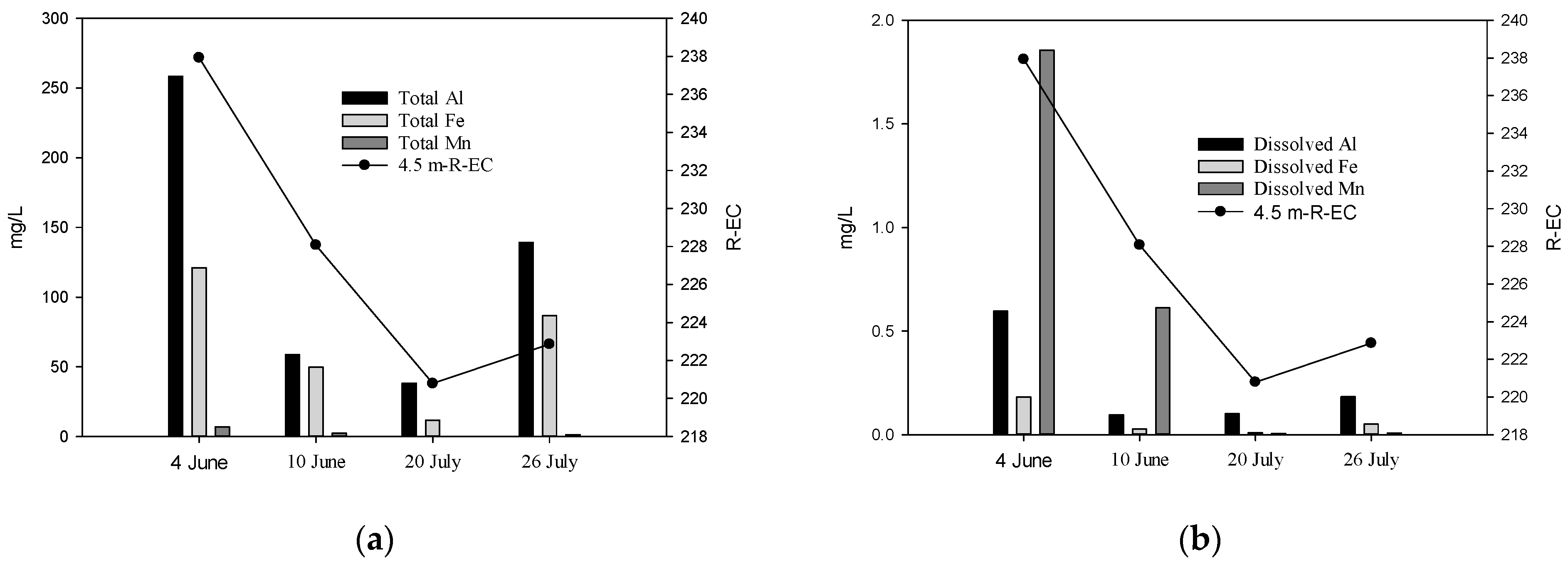
Figure 5 shows that conductivity at 4.5 m was positively correlated with heavy metal concentration. Furthermore, dissolved heavy metals appeared to have a greater influence on conductivity than heavy metals that were adsorbed by flocs, because conductivity increased in step with the dissolved heavy metal concentration. This result is consistent with that shown in Figure 4.
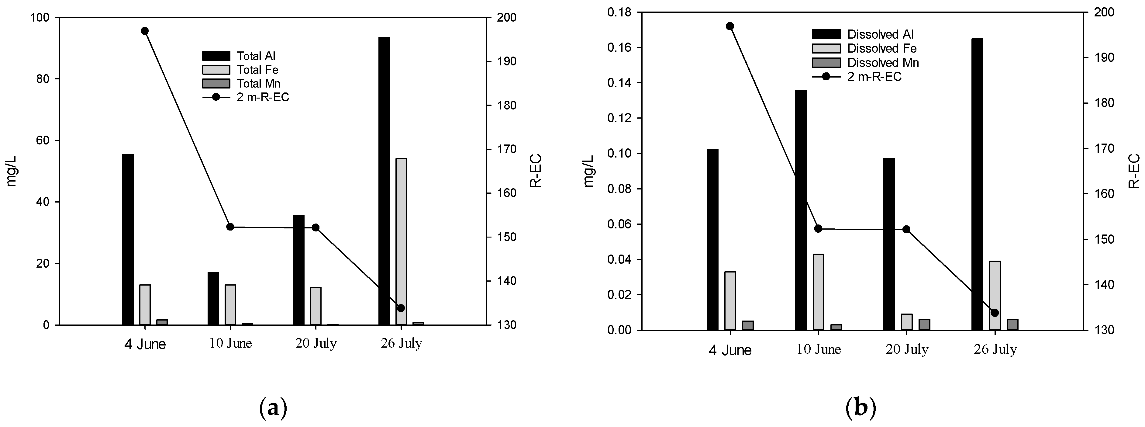
Figure 6 shows that conductivity at 2.0 m was not positively correlated with heavy metal concentration. This result is also inconsistent with that in Figure 4b, which shows that the maximum TDS concentration occurred on 4 June. The dissolved heavy metal concentration on 4 June was also similar to that on other days. Therefore, in addition to dissolved heavy metals (i.e., Fe, Mn, and Al), the water on 4 June also contained other types of conductive dissolved matter.
As Figure 5 already proves that dissolved heavy metals have a greater influence on conductivity than sludge-adsorbed heavy metals, the results in Figure 6 indicate that other dissolved matter, which has an effect on conductivity, was also present in the water. We speculate that these conductive dissolved species were ionic species that were introduced by the addition of PAC, such as OH−, NH3-N, and SO42−.
According to Table 3, the dissolved Mn concentration in the outflow channel on 4 June exceeded drinking water quality standards. In the period 4–10 June, the drought turned to flood. Therefore, the dissolved heavy metals in water gradually decreased with time.
3.2.3. pH
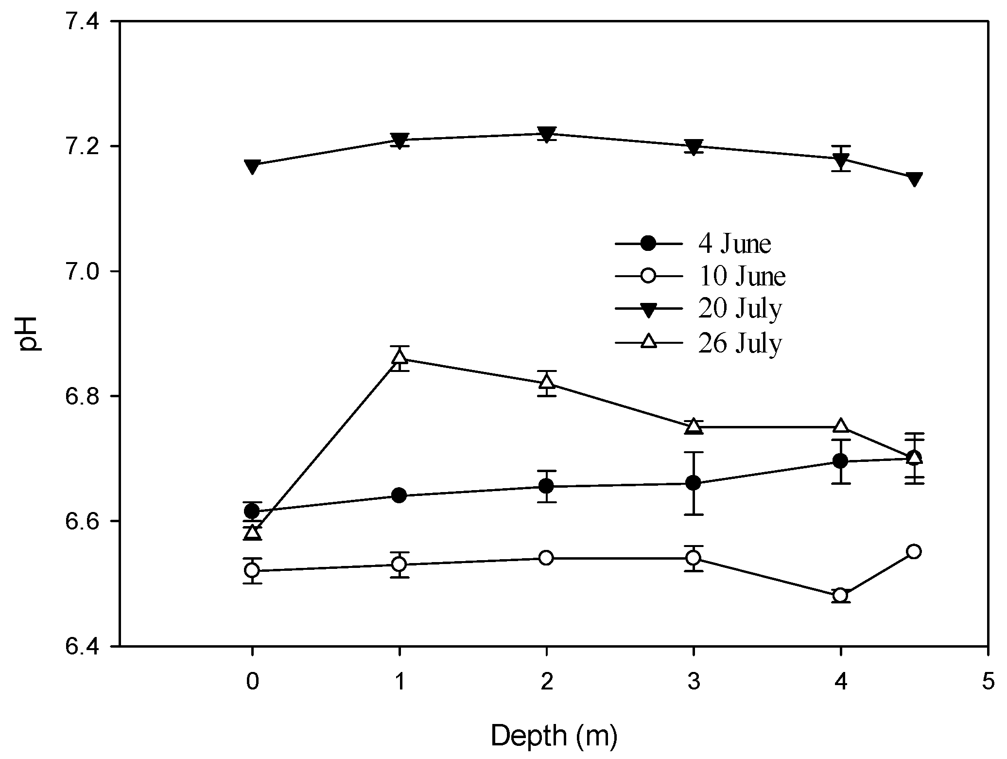
According to Figure 7, the pH of the pond was less than 6.8 on all days except for 20 July. Among the three other days, only on 26 July the pH was 6.8, which indicated that the alkalinity of the water was sufficiently high for floc formation on that day. The pH values on 4 June and 10 June were both less than 6.7; because the concentration of dissolved Al was also high on both of these days, it is likely that the low alkalinity of the pond greatly increased the probability of floc rupture. To elucidate the cause of these pH changes, the pH of the raw waters must be compared to the PAC dosage on each day.
3.3. Raw Water Quality of the Shihmen Dam
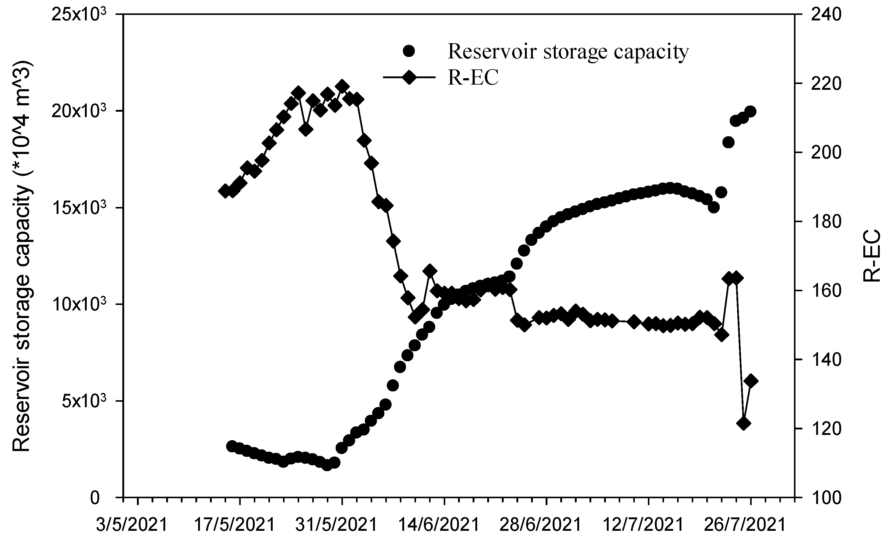
Figure 8 shows that the water level of the Shihmen Dam was low from 15 May until the end of May because the drought was ongoing. The drought ended at the beginning of June when the Meiyu front brought large amounts of rainfall to Taiwan. Typhoon In-fa landed from 22 July to 24 July, which caused intense rainfall over a very short period. Both of these rainfall events caused the turbidity and water level of the Shihmen Dam to increase rapidly.
The PAC dosage is based on the turbidity of raw waters; however, the high-turbidity raw waters caused by these events had different effects on the conductivity of waters inside the HFSBC pond. Therefore, we compared the amount of PAC added by operating personnel during each of these high-turbidity events. Figure 8 may help us to understand how the decisions made by the operating personnel differed in each event with respect to turbidity and PAC dosage.
4. Discussion
Based on the water storage levels, turbidities, PAC dosages, rainfall, and raw-water pH levels shown in Figure 8 and Figure 9, it may be surmised that the period from 15 May to 31 May was the drought period because the water storage level was only 8%. From 31 May to 24 June, the raw-water pH decreased to below 7.50 (below 7.35 from 31 May to 7 June) and then returned to 7.80 on 25 June after the water storage levels increased owing to rainfall from the Meiyu front.
During the transition from the dry season to the wet season, the waters in a reservoir are likely to undergo significant changes in pH and alkalinity. Large amounts of bottom sediment will also be resuspended by the change in water level, which may lead to the release of heavy metal ions that were previously adsorbed by the bottom sediment [18,19], which then enter the water treatment plant via raw water. The results shown in Figure 4, Figure 5, Figure 6 and Figure 7 are generally consistent with this behavior.
Wei et al. [20] noted that the addition of PAC coagulant will consume OH− and thus decrease the pH. Furthermore, if the final pH after PAC addition is poorly controlled and the OH− concentration is not sufficiently high to allow floc settling, the pH will decrease as the PAC dosage increases and thus cause poor coagulation performance.
Figure 9b shows that the raw waters of the reservoir usually had a pH of approximately 7.8. However, the raw-water pH decreased to 7.24 on 1 June, which indicated that the OH− concentration was low at this point. The corresponding PAC dosage was approximately 28.67–57.15 ppm. Based on the conductivity changes in the clear-water layer (Figure 8), the conductivity was high on this day. Thus, we speculated that the PAC dosage was too high because it caused the conductivity of the clear-water layer to reach 220 R-EC. When rainfall caused the water level in the dam to increase from 1 June to 11 June, the raw-water pH also increased steadily during this period, which indicated that the OH− concentration in the raw water was increasing. This was accompanied by a decrease in the heavy metal content in the water. Furthermore, although the PAC dosage was greater than 55.19 ppm, the conductivity of the clear-water layer still decreased to less than 150 R-EC.
As the water level of the dam continued to increase, the turbidity of the raw water also decreased. On 23 July and 24 July, the raw-water turbidity was only 3.2 NTU and 3.9 NTU, respectively, and the raw-water pH had returned to 7.8. However, the conductivity of the clear-water layer was still increasing. We speculate that this occurred because no PAC needed to be added at this point. As the PAC dosage was maintained between 3.67 ppm and 10.67 ppm, there was an excessive amount of residual PAC in the pond, which led to high conductivity in the clear-water layer. This is consistent with the clear-water layer conductivity shown in Figure 8. When the typhoon from 25 July to 26 July brought highly turbid raw waters, the PAC dosage reached 58.8 ppm, but the conductivity still decreased to values between 120 R-EC and 135 R-EC. Because the conductivity did not increase, it was implied that the high PAC dosages still led to effective floc formation.
Because the addition of PAC would consume OH− in raw water, it is possible that the OH− concentration of the raw water was low during the drought period. Therefore, PAC addition caused the pH of the clear-water layer to fall below 6.6 (Figure 7), which precluded effective floc formation. This led to high conductivity and high dissolved Al concentrations. However, after the rainfall events, the OH− concentration of the raw water increased to a point where PAC addition only reduced the pH of the clear-water layer to 6.8. Under these circumstances, PAC addition led to effective floc formation and very low dissolved Al concentrations in the clear-water layer. Furthermore, the conductivity of the clear-water layer remained at approximately 120–135 R-EC.
5. Conclusions
Based on all the data collected in this study, it is clear that the quality of raw water from the Shihmen Dam was significantly affected by drought. By analyzing the total heavy metal concentrations at each depth of the HFSBC pond, it was found that the raw waters contained high concentrations of heavy metals. The addition of PAC was effective in capturing heavy metals in the water, but the SS concentration at the bottom of the pond (4.5 m) was positively correlated with the 4-day average turbidity. We speculated that this was caused by ineffective sludge discharge from the pond and that the sludge degraded and broke up after 4 days in the pond, thereby causing the release of heavy metals from the flocs. This led to a high concentration of dissolved heavy metals in the overflow channel on 4 June. However, the increase in OH− from the rain eventually increased the effectiveness of the PAC coagulant, which then caused the concentration of heavy metals in the clear-water layer to decrease rapidly.
Therefore, the acute degradation in water quality (high heavy metal concentration) was caused by inadequate sludge discharge, which led to the release of heavy metals from degraded sludge. Nonetheless, the water treatment plant could cope with this temporary water quality anomaly by using its large water output to dilute the heavy metals. However, long-term water quality problems, such as those caused by the 2021 drought, when aggravated by sludge discharge problems, will lead to excessive sludge retention times. This may then lead to the release of heavy metals due to sludge degradation.
Coagulation, flocculation, and settling are the only processes that are currently available to water treatment plants for heavy metal removal. If we do not pay adequate attention to problems related to the removal of heavy metals, then end users will suffer from water quality problems such as yellow-colored tap water. Raw waters in Taiwan are known to exhibit great changes in water quality. For instance, their turbidity can range from <5 NTU during the dry season to 1740 NTU when a rainfall event occurs. When faced with such a great change in water quality, treatment plant operators must use their experience to judge the amount of coagulant addition because there are no monitoring devices that can provide supporting information for these decisions. However, the RPMS system has the potential to make water quality predictions and determine the optimality of coagulant dosage. Unfortunately, this system has yet to achieve the level of precision needed to determine the effects of sludge on water quality. Furthermore, it must be enhanced with other water quality sensors to measure sludge blanket thickness and thus quantify the concentration of SS to inform sludge discharge decisions.
Author Contributions
Conceptualization, C.-I.W.; methodology, C.-I.W.; software, H.-C.C.; validation, C.-I.W. and S.-L.L.; formal analysis, C.-I.W.; investigation, C.-I.W.; resources, S.-L.L.; data curation, S.-L.L.; writing—original draft preparation, C.-I.W.; writing—review and editing, S.-L.L.; visualization, C.-I.W.; supervision, S.-L.L.; project administration, S.-L.L.; funding acquisition, S.-L.L. All authors have read and agreed to the published version of the manuscript.
Funding
This work was financially supported by the National Taiwan University (NTUCCP-110L901003, NTU-110L8807) and NTU Research Center for Future Earth from The Featured Areas Research Center Program within the framework of the Higher Education Sprout Project by the Ministry of Education (MOE) in Taiwan and the Ministry of Science and Technology of the Republic of China (MOST110-2621-M-002-011, MOST111-2622-8-002-015-TE2).
Institutional Review Board Statement
Not applicable.
Informed Consent Statement
Not applicable.
Data Availability Statement
Not applicable.
Acknowledgments
The authors would like to thank Wei-Hong Lin, Ting-Yun Hsieh, Yueh-Feng Li of the Department of Environmental Engineering of National Taiwan University for providing constructive comments. The authors also recognize Xuan-Hua Wang and Tsung-Kuei Kuo from the Second Branch of Taiwan Water Corporation for their help with sampling and laboratory measurements.
Conflicts of Interest
The authors declare no conflict of interest.
References
- Peng, C.; Huang, Y.; Yan, X.; Jiang, L.; Wu, X.; Zhang, W.; Wang, X. Effect of overlying water pH, temperature, and hydraulic disturbance on heavy metal and nutrient release from drinking water reservoir sediments. Water Environ. Res. 2021, 93, 2135–2148. [Google Scholar] [CrossRef] [PubMed]
- Gmitrowicz-Iwan, J.; Ligęza, S.; Pranagal, J.; Kołodziej, B.; Smal, H. Can climate change transform non-toxic sediments into toxic soils? Sci. Total Environ. 2020, 747, 141201. [Google Scholar] [CrossRef] [PubMed]
- Ochoa-Contreras, R.; Jara-Marini, M.E.; Sanchez-Cabeza, J.-A.; Meza-Figueroa, D.M.; Pérez-Bernal, L.H.; Ruiz-Fernández, A.C. Anthropogenic and climate induced trace element contamination in a water reservoir in northwestern Mexico. Environ. Sci. Pollut. Res. 2021, 28, 16895–16912. [Google Scholar] [CrossRef] [PubMed]
- Kwok, K.W.H.; Batley, G.E.; Wenning, R.J.; Zhu, L.; Vangheluwe, M.; Lee, S. Sediment quality guidelines: Challenges and opportunities for improving sediment management. Environ. Sci. Pollut. Res. 2014, 21, 17–27. [Google Scholar] [CrossRef] [PubMed]
- Dayananda, N.R.; Liyanage, J.A. Quest to Assess Potentially Nephrotoxic Heavy Metal Contaminants in Edible Wild and Commercial Inland Fish Species and Associated Reservoir Sediments; a Study in a CKDu Prevailed Area, Sri Lanka. Expo. Health 2021, 13, 567–581. [Google Scholar] [CrossRef]
- Palma, P.; Penha, A.; Novais, M.; Fialho, S.; Lima, A.; Mourinha, C.; Alvarenga, P.; Rosado, A.; Iakunin, M.; Rodrigues, G.; et al. Water-Sediment Physicochemical Dynamics in a Large Reservoir in the Mediterranean Region under Multiple Stressors. Water 2021, 13, 707. [Google Scholar] [CrossRef]
- Česonienė, L.; Mažuolytė-Miškinė, E.; Šileikienė, D.; Lingytė, K.; Bartkevičius, E. Analysis of Biogenic Secondary Pollution Materials from Sludge in Surface Waters. Int. J. Environ. Res. Public Health 2019, 16, 4691. [Google Scholar] [CrossRef] [PubMed] [Green Version]
- Zhou, Y.; Liu, M.; Zhou, L.; Jang, K.-S.; Xu, H.; Shi, K.; Zhu, G.; Liu, M.; Deng, J.; Zhang, Y.; et al. Rainstorm events shift the molecular composition and export of dissolved organic matter in a large drinking water reservoir in China: High frequency buoys and field observations. Water Res. 2020, 187, 116471. [Google Scholar] [CrossRef] [PubMed]
- Li, X.; Ma, W.; Huang, T.; Wang, A.; Guo, Q.; Zou, L.; Ding, C. Spectroscopic fingerprinting of dissolved organic matter in a constructed wetland-reservoir ecosystem for source water improvement-a case study in Yanlong project, eastern China. Sci. Total Environ. 2021, 770, 144791. [Google Scholar] [CrossRef] [PubMed]
- Beauchamp, N.; Bouchard, C.; Dorea, C.; Rodriguez, M. Ultraviolet absorbance monitoring for removal of DBP-precursor in waters with variable quality: Enhanced coagulation revisited. Sci. Total Environ. 2020, 717, 137225. [Google Scholar] [CrossRef] [PubMed]
- Sun, C.; Fiksdal, L.; Hanssen-Bauer, A.; Rye, M.B.; Leiknes, T. Characterization of membrane biofouling at different operating conditions (flux) in drinking water treatment using confocal laser scanning microscopy (CLSM) and image analysis. J. Membr. Sci. 2011, 382, 194–201. [Google Scholar] [CrossRef]
- Fortunato, L.; Pathak, N.; Rehman, Z.U.; Shon, H.; Leiknes, T. Real-time monitoring of membrane fouling development during early stages of activated sludge membrane bioreactor operation. Process Saf. Environ. Prot. 2018, 120, 313–320. [Google Scholar] [CrossRef] [Green Version]
- Kim, J.; Park, K.; Joo, K. Feasibility of miniature radiation portal monitor for measurement of radioactivity contamination in flowing water in pipe. J. Instrum. 2018, 13, P01022. [Google Scholar] [CrossRef]
- Fujioka, T.; Ueyama, T.; Mingliang, F.; Leddy, M. Online assessment of sand filter performance for bacterial removal in a full-scale drinking water treatment plant. Chemosphere 2019, 229, 509–514. [Google Scholar] [CrossRef] [PubMed]
- Rao, H.; Liu, W.; He, K.; Zhao, S.; Lu, Z.; Zhang, S.; Sun, M.; Zou, P.; Wang, X.; Zhao, Q.; et al. Smartphone-Based Fluorescence Detection of Al3+ and H2O Based on the Use of Dual-Emission Biomass Carbon Dots. ACS Sustain. Chem. Eng. 2020, 8, 8857–8867. [Google Scholar] [CrossRef]
- Kurajica, L.; Bošnjak, M.U.; Kinsela, A.S.; Štiglić, J.; Waite, T.; Capak, K.; Pavlić, Z. Effects of changing supply water quality on drinking water distribution networks: Changes in NOM optical properties, disinfection byproduct formation, and Mn deposition and release. Sci. Total Environ. 2021, 762, 144159. [Google Scholar] [CrossRef] [PubMed]
- Díaz-Alcaide, S.; Sandwidi, W.J.-P.; Martínez-Santos, P.; Martín-Loeches, M.; Cáceres, J.L.; Seijas, N. Mapping Ground Water Access in Two Rural Communes of Burkina Faso. Water 2021, 13, 1356. [Google Scholar] [CrossRef]
- Bouvy, M.; Nascimento, S.M.; Molica, R.J.R.; Ferreira, A.; Huszar, V.; Azevedo, S.M. Limnological features in Tapacurá reservoir (northeast Brazil) during a severe drought. Hydrobiologia 2003, 493, 115–130. [Google Scholar] [CrossRef]
- Kemdirim, E.C. Studies on the hydrochemistry of Kangimi reservoir, Kaduna State, Nigeria. Afr. J. Ecol. 2005, 43, 7–13. [Google Scholar] [CrossRef]
- Wei, N.; Zhang, Z.; Liu, D.; Wu, Y.; Wang, J.; Wang, Q. Coagulation behavior of polyaluminum chloride: Effects of pH and coagulant dosage. Chin. J. Chem. Eng. 2015, 23, 1041–1046. [Google Scholar] [CrossRef]
Figure 1.
Schematic diagram of the RPMS system.

Figure 2.
Experimental setup structure of the HFSBC.

Figure 3.
Results of real-time precision multi-layer sensor monitoring of the high-speed flocculation flat-bottomed sludge blanket clarifier from 15 May 2021 to 26 July 2021.
Figure 3.
Results of real-time precision multi-layer sensor monitoring of the high-speed flocculation flat-bottomed sludge blanket clarifier from 15 May 2021 to 26 July 2021.

Figure 4.
Changes in suspended solids (SS), total dissolved solids (TDS), and R-EC at depths of (a) 4.5 m and (b) 2.0 m.
Figure 4.
Changes in suspended solids (SS), total dissolved solids (TDS), and R-EC at depths of (a) 4.5 m and (b) 2.0 m.

Figure 5.
Changes in water quality at 4.5 m. (a) Changes in total heavy metal concentrations and (b) changes in dissolved heavy metal concentrations.
Figure 5.
Changes in water quality at 4.5 m. (a) Changes in total heavy metal concentrations and (b) changes in dissolved heavy metal concentrations.

Figure 6.
Changes in water quality at 2.0 m. (a) Changes in total heavy metal concentrations and (b) changes in dissolved heavy metal concentrations.
Figure 6.
Changes in water quality at 2.0 m. (a) Changes in total heavy metal concentrations and (b) changes in dissolved heavy metal concentrations.

Figure 7.
pH changes at each depth.

Figure 8.
Water storage levels of the Shihmen Dam and conductivities of the clear-water layer in the high-speed flocculation flat-bottomed sludge blanket clarifier (HFSBC) pond (the average conductivity at 2.0 m is assumed to correspond to the conductivity of the clear-water layer).
Figure 8.
Water storage levels of the Shihmen Dam and conductivities of the clear-water layer in the high-speed flocculation flat-bottomed sludge blanket clarifier (HFSBC) pond (the average conductivity at 2.0 m is assumed to correspond to the conductivity of the clear-water layer).

Figure 9.
(a) Changes in raw-water turbidity and polyaluminum chloride (PAC) dosage and (b) cumulative rainfall and raw-water pH on each day.
Figure 9.
(a) Changes in raw-water turbidity and polyaluminum chloride (PAC) dosage and (b) cumulative rainfall and raw-water pH on each day.


Table 1.
Mean turbidity (in units of NTU) averaged over different numbers of days.
| Days | 1 | 2 | 3 | 4 | 5 | 6 | 7 | 8 | 9 | 10 | |
|---|---|---|---|---|---|---|---|---|---|---|---|
| Date | |||||||||||
| 4 June | 85.0 | 140.5 | 170.7 | 563.0 | 493.2 | 417.5 | 363.0 | 324.8 | 298.2 | 280.3 | |
| 10 June | 378.0 | 477.5 | 409.0 | 346.3 | 302.6 | 276.8 | 249.4 | 242.8 | 241.4 | 391.3 | |
| 20 July | 35.0 | 35.0 | 36.3 | 36.8 | 37.2 | 37.7 | 37.9 | 38.6 | 39.2 | 39.8 | |
| 26 July | 530.0 | 525.5 | 351.4 | 264.5 | 217.8 | 186.9 | 165.2 | 148.9 | 136.7 | 126.8 | |
Table 2.
Variation in sludge concentration (in units of mg/L).
| Depth | 0.0 m | 1.0 m | 2.0 m | 3.0 m | 4.0 m | 4.5 m | |
|---|---|---|---|---|---|---|---|
| Date | |||||||
| 4 June | 3.0 | 5.9 | 336.5 | 980.0 | 1755.0 | 7120.0 | |
| 10 June | 3.1 | 11.1 | 143.3 | 852.7 | 1145.0 | 1560.0 | |
| 20 July | 2.3 | 3.0 | 346.0 | 437.0 | 526.5 | 326.0 | |
| 26 July | 3.6 | 4.8 | 1595.5 | 2180.5 | 1982.5 | 1814.5 | |
Table 3.
Water quality of the outflow channel (in units of mg/L).
| Item | Dissolved Al | Dissolved Mn | Dissolved Fe | |
|---|---|---|---|---|
| Date | ||||
| 4 June | 0.214 | 0.167 | 0.186 | |
| 10 June | 0.201 | 0.003 | 0.056 | |
| 20 July | 0.040 | 0 | 0.004 | |
| 26 July | 0.041 | 0 | 0.013 | |
Publisher’s Note: MDPI stays neutral with regard to jurisdictional claims in published maps and institutional affiliations. |
© 2022 by the authors. Licensee MDPI, Basel, Switzerland. This article is an open access article distributed under the terms and conditions of the Creative Commons Attribution (CC BY) license (https://creativecommons.org/licenses/by/4.0/).
Share and Cite
MDPI and ACS Style
Wu, C.-I.; Lo, S.-L.; Chung, H.-C. Automated Monitoring of a High-Speed Flocculation Flat-Bottomed Sludge Blanket Clarifier Pond during Drought and Flood Conditions. Water 2022, 14, 1170. https://doi.org/10.3390/w14071170
AMA Style
Wu C-I, Lo S-L, Chung H-C. Automated Monitoring of a High-Speed Flocculation Flat-Bottomed Sludge Blanket Clarifier Pond during Drought and Flood Conditions. Water. 2022; 14(7):1170. https://doi.org/10.3390/w14071170
Chicago/Turabian StyleWu, Chun-I, Shang-Lein Lo, and Hsu-Chen Chung. 2022. "Automated Monitoring of a High-Speed Flocculation Flat-Bottomed Sludge Blanket Clarifier Pond during Drought and Flood Conditions" Water 14, no. 7: 1170. https://doi.org/10.3390/w14071170
Note that from the first issue of 2016, this journal uses article numbers instead of page numbers. See further details here.