
An Integrated Approach for Deciphering Hydrogeochemical Processes during Seawater Intrusion in Coastal Aquifers
by
 , , , and
Hend S. Abu Salem
1,* ,
,
Khaled S. Gemail
2 ,
,
Natalia Junakova
3,* ,
,
Amin Ibrahim
2 and
Ahmed M. Nosair
2 1
Geology Department, Faculty of Science, Cairo University, Giza 12613, Egypt
2
Environmental Geophysics Lab (ZEGL), Geology Department, Faculty of Science, Zagazig University, Zagazig 44519, Egypt
3
Department of Environmental Engineering, Faculty of Civil Engineering, Technical University of Kosice, 04200 Kosice, Slovakia
*
Authors to whom correspondence should be addressed.
Water 2022, 14(7), 1165; https://doi.org/10.3390/w14071165
Submission received: 23 February 2022
/
Revised: 31 March 2022
/
Accepted: 2 April 2022
/
Published: 6 April 2022
(This article belongs to the Special Issue Assessment and Management of Hydrological Risks Due to Climate Change)
Abstract
:For managing the freshwater in the worldwide coastal aquifers, it is imperative to understand the hydrogeochemical processes and flow patterns in the mixing freshwater/saltwater zone. The Egyptian Nile Delta aquifer is a typical example. The management of seawater intrusion (SWI) requires detailed investigations of the intrusion wedge and the dynamic processes in the mixing zone. Thus, a multidisciplinary approach was applied based on holistic hydrogeochemical, statistical analysis, and DC resistivity measurements to investigate the lateral and vertical changes in groundwater characteristics undergoing salinization stressor. The results of cross plots and ionic deviations of major ions, hydrochemical facies evolution diagram (HFE-D), and seawater mixing index (SMI) were integrated with the resistivity results to show the status of the SWI where the intrusion phase predominates in ~2/3 of the study are (~70 km radius) and the compositional thresholds of Na, Mg, Cl, and SO4 are 600, 145, 1200, and 600 mg/L, respectively, indicating that the wells with higher concentrations than these thresholds are affected by SWI. Moreover, the results demonstrate the efficiency of combining hydrogeochemical facies from heatmap and resistivity investigations to provide a large-scale characterization of natural and anthropogenic activities controlling aquifer salinization to support decision-makers for the long-term management of coastal groundwater.
1. Introduction
Coastal aquifers undergo several stressors due to global climatic changes, sea-level rise (SLR), the world’s growing population, and increasing developmental activities [1,2,3,4]. The most common stressor is groundwater salinization that is driven by water level decline and SLR [5,6,7,8]. The sources of salinity in coastal aquifers are manifold, including invasion of seawater to the fresh groundwater [9] and mixing with highly saline fossil water [10] or with wastewater [11,12]. Accordingly, coastal aquifers require costly effective management plans to limit freshwater deterioration.
In arid and semi-arid regions, seawater intrusion (SWI) is considered a global issue that restricts groundwater pumping in coastal aquifers. Therefore, understanding complex hydrogeochemical processes and factors that control the evolution of brackish groundwater in coastal aquifers as well as the sources of salinization is crucial. However, the great complexity of coastal aquifers in terms of aquifer heterogeneity, spatial and temporal variations in the flow regime, and surface water–groundwater interactions complicate the interpretation of the controlling factors in fresh–saline water distribution [13]. Numerous studies were implemented to assess SWI in coastal aquifers using different methods—e.g., hydrogeochemical investigations [14,15], geophysical methods [16,17,18,19,20], isotope tracers [21,22,23], and statistical analysis [24,25]. SINTACS, DRASTIC, AVI, and GALDIT models are popular methods for mapping coastal aquifer vulnerability to natural and anthropogenic factors based on hydrogeological and hydrogeochemical parameters (e.g., aquifer type, hydraulic conductivity, water level, electrical conductivity, chloride concentration, Revelle index (Cl−/HCO3− + CO3−2)) [26,27,28,29]. SINTACS, DRASTIC, and AVI are mostly used to determine aquifer vulnerability to surface contamination as wastewater, while the GALDIT is mainly related to seawater intrusion [27,28]. The Nile Delta aquifer is among the foremost important aquifers in the world; however, it suffers from SWI from the northern parts at the Mediterranean Sea because of severe pumping, especially in the central parts of the Nile Delta area [30,31,32]. Sherif et al. [31] demonstrated that seawater has intruded into the Nile Delta aquifer about 100 km from the coast. The seawater interface toe location was at ~23 km in the eastern Nile Delta before the 1950s when pumping from the Nile Delta aquifer was minimal; then, in the 1990s with pumping at 1.92 billion m3/yr [33], the interface surface moved 40 km landward. In the year 2000, with the pumping of 2.4 billion m3/yr, the interface moved 116 km landward from the coastal line in the eastern Nile Delta [31,32].
Previous studies on the Nile Delta aquifer system have involved hydrogeologic and hydrogeochemical studies dealing with SWI [15,30,34,35]. These studies described the extent of SWI into the aquifer, in addition to using vulnerability mapping and mathematical simulation for seawater encroachment to the aquifer. However, there is still a gap in understanding the hydrochemical processes during SWI into the aquifer. From this point of view, the present work aimed to understand the hydrogeochemical processes occurring during the groundwater–saline water mixing process as well as the origin of solutes and sources of salinity. To fill this knowledge gap, a holistic study using hydrogeochemical indicators, multivariate statistical analysis, and geophysical mapping was proposed to delineate and explain the chemical changes of the groundwater due to SWI.
The assessment of aquifer vulnerability to saltwater intrusion or pollutants using water sampling from wells is a reliable tool for monitoring water quality due to the seawater intrusion based on the total depth of the collected samples. However, unplanned wells with different depths cannot configure the continuity of the freshwater/saltwater full interface and may be difficult when attempting to understand the intrusion mechanism in the coastal aquifers. In such cases, surface geophysical methods such as the vertical electrical resistivity (VES) offer a potentially valuable, non-destructive, and cost-effective tool for mapping the seawater interface, where the electrical properties of the freshwater and seawater show large contrast in resistivity values.
The proposed approaches include hydrogeochemical analysis using ionic deviations of major ions, hydrochemical facies evolution diagram (HFE-D), groundwater quality index for seawater intrusion (GQISWI), seawater mixing index (SMI), and multivariate statistical analysis. Additionally, geophysical measurements were employed to validate the hydrogeochemical results and to delineate the vertical boundary of the fresh/saltwater interface. Finally, the geospatial distribution of the different parameters was addressed for visual investigation. The integration between these approaches will add valuable information and understanding of SWI in the Nile Delta aquifer system and can be applied in similar circumstances elsewhere as a good qualitative practice for coastal aquifers management.
1.1. Study Area
The study area is represented by the Sharkia Governorate in the Eastern part of the Nile Delta of Egypt. It is located between longitudes 31°15′30.7″–32°10′28.71″ E and latitudes 30°9′17.84″–31°10′2.91″ N (Figure 1) and is characterized by arid to semi-arid climate and has low relief surface sloping gently toward the north direction [15]. The ground surface is covered mainly by deltaic sediments that are used in different agricultural activities and dissected by a large network of freshwater canals and drainage systems [36]. It is bounded from the north by El-Manzala Lake, which represents the main source of SWI to the Nile Delta aquifer, especially with severe pumping of the groundwater [34,36].
1.2. Geological and Hydrogeological Setting
The study area is covered mostly by the Quaternary sediments with varying thickness. It is composed of sand, silt, gravel, clay, silty, and sandy clay deposits with lateral discontinuity [37]. The Quaternary sediments are underlain by the older Pliocene clays in most parts of the study area, while it is underlain by the Miocene and Oligocene deposits in the east and south parts [37]. These deposits form the Nile Delta aquifer that represents the main groundwater-bearing unit in the study area (Figure 2).
The Nile Delta aquifer is classified into an Upper Holocene clay cap unit and a Lower Pleistocene aquifer unit, which represents the main groundwater storage unit in the study area. The Pleistocene unit is classified based on lithology into Late and Early Pleistocene units that vary in thickness from 200, 500, and 800 m in the south, central, and northern parts of the study area, respectively [39] (Figure 2a). The Late Pleistocene aquifer is overlain directly by the Holocene clay cap unit and formed of medium sand with intercalations of clay lenses with an average thickness of 50 m. It is underlain by the Early Pleistocene aquifer unit, which is composed of coarse sand and gravels with clay intercalations. These two units are hydraulically connected and not easily differentiated, especially when the Holocene clay cap is missing in some parts of the Nile Delta [37]. The Holocene layer is composed of silt, clayey sand, and sandy clay, with fine sand intercalations. Its thickness varies from about 5 m and 70 m in the southern and northern parts, respectively (Figure 2b,c). It acts as an aquitard layer in the southern and central parts, while it acts as an aquiclude layer in the northern parts. The aquifer is recharged through the seepage from the distributed network of irrigation canals cutting the Holocene layer, as well as the Ismailia Canal that runs in the Pleistocene sediments. The groundwater levels in this aquifer decreased from southern (water level: 8–14 m asl) to northern parts (water level: <1 m asl) of the study area, with general flow direction from the south to the north and northeast directions [40] (Figure 2b).
2. Materials and Methods
Groundwater samples were collected through the year of 2018 from 60 drilled wells with variable total depths (18–120 m below the ground surface). Each well was pumped for about 20 to 30 min before sampling. On-field measurements were made after stabilization of the meter readings to determine the total dissolved solids (TDS), electrical conductivity (EC), and pH, using standard calibrated Orion portable meters. Each groundwater sample was added to polyethylene bottle after cleaning well with water sample at the sampling location. The concentration of HCO3− was measured by titration method using H2SO4 (0.01 normality). The concentrations of the other major anions and cations were detected using ion chromatography (Dionex, ICS-1100) (Table S1).
The hydrogeochemical processes prevailing during SWI were investigated using the groundwater quality index for seawater intrusion (GQISWI), ionic deviations, seawater mixing index (SMI), Piper diagram, hydrochemical facies evolution diagram (HFE-D), binary diagrams, and statistical analysis. The obtained results were further validated using geophysical tools.
2.1. Groundwater Quality Index for Seawater Intrusion (GQISWI)
The GQISWI is an index developed by [41] to facilitate the geospatial analysis of groundwater quality (in terms of seawater salinization) rather than traditional pattern diagrams. It is calculated according to [42] as in Equations (1)–(3):
where GQIPiper (mix) is the freshwater seawater mixing index of the piper diagram; GQIfsea is seawater fraction index.
GQIPiper(mix) = (Ca2+ + Mg2+ + HCO3−) × 50 (in % meq/L)
GQIfsea = (1 − fsea) ×100
The seawater fraction (fsea) is calculated using the Cl− concentration of the sample, where Cl− is considered as a conservative parameter. Accordingly, the fraction of seawater is calculated as follows:
If Cl− is only derived from seawater, then mCl, fresh should equal to zero so that
where the denominator is equal to the concentration of Cl− in mmol/L of 35‰ (grams of salt per kilogram) seawater [41,43].
2.2. Ionic Deviations (mi, react)
The chemical reactions taking place during fresh/seawater interaction could be deduced by calculating the expected ions’ compositions based on conservative mixing of saltwater and freshwater, and then comparing the result with the measured concentrations in the water sample [43]. Thus, the concentration of an ion (i) by conservative mixing of seawater and freshwater is
where mi is the concentration of i (mmol/L), fsea is the fraction of seawater in the mixed water, and subscripts mix, sea, and fresh indicate a conservative mixture, seawater, and freshwater, respectively. Any change in the concentration mi, react due to reactions then becomes simply
Thus, the calculated difference or ionic deviations (mi, react) between the mixed (mi, mix) and the measured compositions indicates the possible reactions [43] where the Cl is used in these calculations due to its conservative nature. The use of ionic deviations in hydrogeochemical modeling better explains the possible reactions rather than the original concentrations.
The ionic deviations of the major ions were used considering sample 57 as the fresh groundwater endmember where it is characterized by Ca-HCO3 water type, lowest Cl, and lower TDS concentrations and is representative of the fresh surface water of the River Nile and the Ismailia freshwater canal (Table S2).
2.3. Hydrochemical Facies Evolution Diagram (HFE-D)
This diagram was used to study the hydrogeochemical changes in groundwater experiencing salinization–freshening phases in coastal aquifers [44,45]. It is used as an alternative to other hydrochemical diagrams, yet it has more benefit as it helps in the identification of the hydrochemical facies without amalgamations (parts of the diagram necessarily representing two or more different ions, e.g., Piper and Durov diagrams). In addition, it permits visualization of possible groupings of samples and trends of evolution occurring in the aquifer [46,47,48,49]. In this diagram, the abscissa reproduces cation percentages and their evolution, considering the two most important cations (%Na and %Ca (or %Mg)) that interpret base-exchange reactions while the ordinates denote the mixing process, where %HCO3 (for recharge waters with a bicarbonate facies) or %SO4 (for recharge water with a sulfate facies) indicate the dominant anion in the recharge water. Details about the different hydrochemical facies in the HFE diagram are given in [44], where four heteropic facies—NaCl, CaCl2, NaHCO3, and CaHCO3—are defined and each heteropic facies is represented by four other subfacies that are similar to them. Accordingly, sixteen isopic facies could be extracted from the diagram. The main hydrochemical processes occurring during seawater intrusion could be recognized by the excess or deficit compared with the line of conservative mixing between freshwater and seawater (conservative mixing line (CML)) in the freshening and intrusion stages, respectively.
The isopic facies that are related to freshening substages are f1 to f4, while those of the intrusion substages are i1 to i4. The i1 and f1 substages characterize the distal facies that define the boundary between the two invasive flows where this boundary must not be mistaken with the conservative mixing line represented in the HFE diagram. On the contrary, the proximal facies are f4 and i4 and are closely linked to the end members FW and SW, while the substages (i2, i3, f2, and f3) represent the intermediate levels where cation exchange is usually more evident. The samples sited in the freshwater field are considered as belonging to the freshening phase, although they are in the intrusion field. Similarly, samples located in the saltwater field represent the intrusion stage, even if they are in the freshening field [44].
The endmembers of seawater (SW) and freshwater (FW) can be theoretical or actual [50]. The FW endmember should be critically selected as all processes are evaluated from the starting point of the seawater–freshwater mixing line, and the only variable is the recharge water because seawater is considered stable [51].
2.4. Seawater Mixing Index (SMI)
The seawater mixing index (SMI) estimates the degree of seawater mixing [52], where the major ionic constituents of seawater (Cl−, SO42−, Na+, and Mg2+) were used to calculate this index (Equation (8)).
where a, b, c, and d are constants representing the relative concentration proportion of Na+, Cl−, Mg2+, and SO42− in seawater where their values are 0.31, 0.04, 0.57, and 0.08, respectively. C represents the measured concentration of these ions in mg/L, where T signifies the values of regional threshold of the measured ions, which can be calculated by using the cumulative probability curves and where the inflection points in the curves were used for the concentrations of Cl−, SO42−, Mg2+ and Na+ in groundwater samples [53]. Samples of SMI value greater than 1 characterize groundwater affected by seawater–freshwater mixing process, where SMI values lower than 1 signify freshwater.
2.5. Base Exchange Index (BEX)
The BEX was used to assess a dolomite-free aquifer system experiencing freshening or salinization; Stuyfzand [54] defined this index as BEX = Na+ + K+ + Mg2+ − 1.0716Cl− (meq/L). A positive BEX represents freshening, a negative BEX represents salinization, and a BEX of zero indicates no base exchange.
2.6. Sodium Adsorption Ratio (SAR)
This parameter is used as an indicator of the salinity hazard. High values imply a hazard of the water to the soil. It represents the amount of sodium relative to calcium and magnesium in the water extract from saturated soil (Equation (9)).
SAR = Na/(Ca + Mg/2)^ 0.5
2.7. GIS Spatial Mapping
The measured data were used to build a geodatabase inside ArcGIS 10.3 software (Esri, Redlands, CA, USA) [55]. The locations of the collected samples were geo-referenced, converted to shapefile format, and interpolated to produce spatial distribution maps of the studied parameters in a raster format. These maps were produced using the Kriging interpolation method inside GIS Spatial Analyst Tool [55,56,57]. Kriging is a multistep procedure that comprises exploratory statistical data analysis, variogram modeling, and surface creation (Figure S1). Kriging is an advanced and accurate interpolation geostatistical procedure, and it is commonly used in soil, water resources, and geology sciences [55].
2.8. Geophysical Measurements
Electrical resistivity can be used as an indicator of SWI, where electrical conductivity (the inverse of electrical resistivity) is based mainly on the amount of TDS in groundwater. In the coastal aquifers as in the Nile Delta, the low resistivity anomalies of less than 2 Ωm indicate a seawater intrusion zone [16]. The authors of [27,34] carried out a DC resistivity survey to study the effect of pumping on SWI in the eastern and central Nile Delta, respectively. Their results categorized the groundwater into three classes based on the TDS concentration and resistivity values: 1) freshwater (35–100 Ωm), brackish water (5–35 Ωm), and saltwater (1–8 Ωm). Accordingly, the surficial DC resistivity surveys, accompanied with limited hydrochemical data are widely used for mapping subsurface problems relevant to groundwater quality to describe the spatial distribution of freshwater and saltwater in coastal regions [27,58,59,60,61]. Reasonably, the vertical electrical sounding (1D-VES) measurements were collected at 49 sites using Schlumberger array to validate the existing freshwater boundary identified through the hydrochemical facies modeling and calculated SMI at different depths. The VES technique outlines the vertical variation of the electrical resistivity and can easily detect the freshwater–saltwater interface compared with the traditional water sampling [62]. Basically, during the field work, an electrical current was released into the ground between a pair of steel electrodes (A and B), and voltage was measured between another two electrodes to estimate the subsurface electrical resistivity distributions. The subsurface electrical resistivity has generally been deployed to identify subsurface layer distributions and groundwater potentialities at depths that vary between a few meters up to hundreds of meters. The maximum current spacing (AB) ranges from 300 m near El Manzala Lake in the north to 800 m in the southern part of the surveyed area. According to the available geological information, the applied spreading is long enough to penetrate the expected fresh/seawater interface. Some of the measured soundings were conducted close to some existing shallow wells to define the parametric resistivities of the subsurface layers and the depth to the water table. The collected apparent resistivities and AB/2 measurements were inverted into layer resistivities and thicknesses using the IPI2WIN 3.01software [63]. The inversion results show the vertical variations in the soil and water quality; therefore, it can map the interfaces of freshwater and saltwater more precisely, as seen in Figure 3.
3. Results and Discussions
3.1. Groundwater Classification and Salinity
The studied groundwater samples were classified on the basis of GQISWI values (Table S1) into highly fresh ‘FGH’ (GQISWI > 80; 4 samples), slightly fresh ‘FGS’ (GQISWI from 75 to <80; 11 samples), slightly mixed ‘MGS’ (GQISWI from 70 to <75; 5 samples), fairly mixed ‘MGF’ (GQISWI from 65 to <70; 11 samples), highly mixed ‘MGH’ (GQISWI from 60 to <65; 8 samples), extremely mixed ‘MGE’ (GQISWI from >50 to <60; 12 samples), and saline groundwater ‘SG’ (GQISWI from 10–50; 9 samples) (Table S1). For simplicity, we used acronyms to describe the different groundwater classes where FG, MG, and SG are for fresh groundwater, mixed groundwater, and saline groundwater, respectively. The third letter of the acronym denotes the first letter of the water class. The groundwater salinity distribution is spatially comparable with the GQISWI distribution (Figure 4). Additionally, the composition of the groundwater samples was investigated using a Piper diagram [42], where it evolves from Ca-HCO3 and Na-HCO3 (in the south) to mixed Mg-Na-Ca-Cl-HCO3 and mixed Na-Ca-Mg-HCO3-Cl, to Na-Cl and Na-Cl-SO4 (in the central parts), and finally to Mg-Na-Cl water types (in the north) (see zones A, B, and C in Figure 5). The dominant groups, Na-Cl and mixed Mg-Na-Ca-Cl-HCO3, dominate the northern and central parts of the study area, where the Ca-HCO3 and Na-HCO3 water types characterize samples of the southern parts, where it has very low concentrations of TDS and Cl. In general, Na-Cl and Mg-Na-Cl-type waters reflect the higher influence of seawater in intrusion in coastal aquifers [43,64]. Additionally, the conservative mixing line between sample 57 (freshwater endmember) and seawater (the Mediterranean Sea water of [65,66]) was shown on the Piper diagram (Figure 5), where the plotting of samples above this line indicates the effect of salinization, while those below this line indicate freshening processes.
3.2. Descriptive Statistics and Coefficient of Variation
The studied variables show very wide ranges and high standard deviations (Table 1). In particular, the TDS and EC values have a wide range, with means 3595 ppm and 5429 μS/cm and standard deviations of 5397 and 8135, respectively (Table 1). Similarly, the ranges and standard deviations of K, Na, Mg, Ca, SO4, and HCO3 ions are also wide, indicating that complex hydrogeochemical processes and/or multiple sources could be responsible for the composition of these waters (Table 1).
To confirm the variable sources of ions, the coefficient of variation (CV) was calculated for the studied variables (Table 1). Generally, it is applied to express the precision and repeatability of a geochemical analysis [67]. The CV represents the ratio of the standard deviation (SD) of an element to its average concentration, giving a standardized measure of the dispersion of a probability or frequency distribution [68]. Generally, a CV near zero indicates that the population is homogeneous (Table 1). Accordingly, the TDS, EC, and the major ion concentrations have higher CV values representing the heterogeneity of these variables and confirming multiple sources of mineralization. Additionally, the log-normal distribution of K, Ca, Mg, Cl shows a tail at the high concentration ranges, while most ions show a polymodal distribution, where the population of higher concentrations is possibly attributed to seawater mixing (Figure 6).
3.3. Pearson’s Correlation and Hydrogeochemical Reactions
Pearson’s correlation analysis [69] assesses the correlation between different variables in a system. Several studies focused on the ion exchange of major cations (Na+, K+ Ca2+, Mg2+) in coastal aquifers [43,70,71], where the major hydrogeochemical processes could be identified. Additionally, cross plots of major ions were used to decipher the hydrogeochemical reactions operating in aquifers [72,73,74,75]. In this study, integration between the results of Pearson’s correlation and cross plots were made to study the possible sources of ions in the studied groundwater samples (Table S3; Figure 7). Generally, when seawater intrudes fresh groundwater, Na+ is adsorbed on clay surfaces in the aquifer matrix and Ca2+ is released into the water leading to change of Na-Cl water type to the Ca-Cl2 water type [64]. On the contrary, aquifer freshening is indicated by Na-HCO3 water type, where ion exchange between Ca in the water and Na on the clay matrix occurs.
The correlation was applied to selected variables (total depth, water level, pH, EC, distance from shoreline, and Cl), saturation indices (SIHal, SIGyp, SIDol, SICal), SAR, BEX, and the calculated ionic deviations (m HCO3-react, m SO4-react, m Ca-react, m Mg-react, m Na-react, m K-react) (Table S3). A correlation factor r ≥ 0.5 indicates a significant level of correlation and is used in this work to preliminarily evaluate the main source of salinity based on the used variables [76,77].
The Cl contribution to groundwater salinity is evidenced by the strong linear relationship between Cl and TDS (Table S3, Figure 7a). However, the samples of the MGE and SG lie slightly above the theoretical mixing line between freshwater (sample 57) and seawater (Figure 7a), indicating that the salinity of groundwater is derived not only from marine sources but also from other sources (e.g., anthropogenic sources from drains and return flow of evaporated surface water (Figure 7a). Na+, K+, and Mg2+ correlate well with Cl− for most groundwater types at Cl− < 150 epm (Figure 7b–d). At higher Cl− levels (the SG water samples), Na+ and Mg2+ show deficit and surplus, respectively, suggesting reverse ion exchange prevailing during the seawater intrusion. This is also confirmed by the strong negative correlation between EC and Cl with reacting sodium and potassium (Table S3). Few samples plot along the 1:1 line, indicating possible halite dissolution (Figure 7b), while most samples lie slightly above and below the 1:1 line, indicating the possibility of silicate weathering and/or anthropogenic effects, respectively [78], (Figure 7b). Halite dissolution could be due to the occurrence of several clay lenses in the Quaternary aquifer [37]. Additionally, the variable sources of Na+ and Cl− could also be deciphered from the relation between Na+ + K+ and Cl−+ SO42− (Figure 7k). In this relation, the continuous increase in these ions along the 1:1 suggests a geogenic origin [79]; however, the concentrations of these elements in the studied samples do not fall along the 1:1 line (Figure 7k), indicating other sources. Mg2+ and Ca2+ show excessive concentrations for the MGF, MGH, MGE, and SG, where they deviate from the theoretical mixing line between seawater and freshwater (Figure 7e), indicating reverse ion exchange reactions. However, reverse ion exchange is not the only process that drives the hydrochemistry of the mixed groundwater, where the majority of the mixed type groundwater lies below 1:2 line in the relation between HCO3− and Ca2+, indicating possible CO2 dissolution according to reaction 10 or organic matter oxidation that derives the production of CO2 or due to refreshing recharge of surface water (Figure 7h).The increased Ca2+ and HCO3− concentrations in the mixed- and saline groundwater derive the saturation index of calcite and dolomite to positive values that could lead to their precipitation (see the scatter plot in Figure 7f and Figure 8a,b; SMI in the ordinate of Figure 8 will be discussed later). The SO42− concentrations for most samples are exceeding those expected from mixing of seawater and freshwater (Figure 7g), indicating multi-sources.
When SO42− concentrations in groundwater exceed 100 mg L−1, the possible sources are attributed to anthropogenic inputs and/or lithogenic sources (sulfate evaporites, pyrite or organic matter oxidation) [80]. However, gypsum dissolution and iron sulfide oxidation are precluded for the MGE and SG and the possible sources could be related to anthropogenic impacts (Figure 7i,j). Additionally, the ionic deviations of SO42− increase in the MGE and SG as the distance from the shoreline decreases as well as the well depths decrease proposing mixing with seawater (Figure S5c,k). Conversely, samples from distant and deep wells (more than 50 m depth) have low reacting SO42− contents in the mixed groundwater, indicating that the well depth seems not to be influencing the SO42− content in the mixed and fresh groundwaters (Figure S5c,k). The FG and the MGS seem not to be potentially affected by anthropogenic sources of sulfate where the samples plot above the 1:1 line (Figure 7i). Some samples of the MGS and MGF lie along the 1:1 line, suggesting possible evaporite dissolution that is associated with clay lenses in the Quaternary aquifer [37] (Figure 7i). The increase in Ca and SO42− during aquifer salinization drive the saturation index of gypsum to positive values (Figure 8c, Table S2).
The water level shows negative correlation with SIHal (−0.71), SIGyps (−0.67), SAR (−0.57), Cl (−0.56), and EC (−0.56), which explains the dynamics during seawater mixing, as during high water levels, all of these parameters decrease and vice versa (Figure S6e,f,g). Generally, the chemistry of the SG (represented by Na+, Mg2+, and SO42−) is significantly affected by the distance from shoreline, water levels, and well depths. On the other hand, the chemistry of the rest of groundwater samples (represented by Na+, Mg2+, and SO42−) show no definite trend with shoreline, water levels, and well depths (Figure S2).
Another interesting result is the negative correlation between the BEX and Cl (−0.63), BEX and reacting Ca (−0.65), and the positive correlation between BEX with Na and K (0.93, 0.67, respectively), where a positive BEX represents freshening and a negative BEX represents salinization and confirming the cation exchange processes prevailing during aquifer salinization (Supplementary Table S3).
3.4. Factor Analysis
Factor analysis (FA) is a multivariate statistical technique used to quantify the interrelationships among a large number of variables into a smaller set of dimensions with a minimum loss of information [80]. It is used to identify important factors contributing to the groundwater hydrochemical processes [81,82,83,84]. The correlation matrix was created based on standardized data sets. Then, the eigenvalues and factor loadings of the correlation matrix were defined. Factors were extracted when eigenvalues were greater than 1 [85,86].
The sampling adequacy and the feasibility of applying the FA were tested using Bartlett’s sphericity tests and the Kaiser–Meyer–Olkin (KMO) [87] (Table 2). The best adequacy results were obtained using eighteen variables: distance from the shoreline, total depth, water level, pH, EC, TDS, SAR, K+, Na+, Mg2+, Ca2+, Cl−, SO42−, HCO3−, and saturation indices of halite, gypsum, dolomite, and calcite. Accordingly, the KMO test result was 0.79, confirming the adequacy of PCA in reducing the dimensionality of the dataset due to inter-correlation between variables. Additionally, the results from Bartlett’s sphericity test (chi-square = 2604.09; degrees of freedom ‘df’ = 153; and p < 0.001 “=zero”) confirm that there is common variance shared among the studied variables. Based on eigenvalues (more than one) and varimax rotation, three factors were discerned to explain most of the variability, with a total cumulative variance of about 86% for the groundwater samples (Table 2 and Figure S3).
Factor 1 accounts for about 50% of the total variance. It is represented by a strong positive loading on TDS, EC, Mg2+, Cl−, Na+, Ca2+, SO42−, K+, SAR, and saturation indices of halite and gypsum (Table 2). This indicates that the salinity of groundwater is attributed to manifold sources (seawater mixing and possible anthropogenic sources as evidenced by high SO42− and Cl−).
Factor 2 explains about 19% of the total variance, in which a strong negative loading is found on distance (−0.85), total depth (−0.83), and water level (−0.83). Moderate positive loading on SIHal (0.62) and SIGyp (0.54) exist (Table 2). This factor signifies that under conditions of proximity to the shoreline and the existence of shallow wells and lower water levels, the composition of the groundwater changes, being enriched in some elements that derive the saturation indices of gypsum and halite to positive values, representing the effect of seawater mixing on the groundwater quality.
Factor 3 accounts for about 17% of the total variance, where a strong positive loading on SIDol (0.96) and SICal (0.96), HCO3− (0.81), and pH (0.69) exist. This factor represents the freshening and water–rock interaction factor that characterizes sample populations close to the Ismailia freshwater canal due south of the study area.
3.5. Spatial Distribution of Groundwater Facies
The seawater contribution in the studied samples ranged from 0% in sample 57 to ~48% in sample 33 (Table S2). The plot of the calculated ionic deviations for Na and Ca (and Mg) against chloride concentrations shows the onset of cation exchange reactions in the aquifer at Cl concentrations (more than 500 ppm, Figure 9). The degree of seawater contribution in the groundwater samples was studied using an HFE diagram and SMI. In this diagram, sample 57 was used to represent the FW endmember, while the Mediterranean water was used as the SW endmember [65,66].
The distribution of hydrogeochemical facies of the studied samples in the HFE-D shows that water samples influenced by SWI are represented by red color, while samples representing freshwater are in green color (Figure 10a). Ten hydrochemical substages are recognized representing the freshening stage (24 samples representing 40.7% of the total samples) and intrusion stage (35 samples representing 59.3%). Details on the percentages and facies of each substage are given in (Table S4). The freshening phase of the studied samples starts from an initial situation in which the aquifer is totally salinized by seawater ingress. Going from inland to the coast, the recharge water from surface canals begins to rinse the aquifer that is in equilibrium with the Na-Cl facies and is represented by the distal freshening facies ‘f1’ (MixNa-Cl, representing MGF, MGH, and MGE; samples 58, 2, 4, 32, 13, 18, 26, 30, 31; see Table S1 for classification, Figure 10a). After that, the water evolves to substages ‘f2’ (MixNa-MixCl, representing MGF, MGH, and MGE and encompassing samples 25, 54, 55, 17, 56) and ‘f3’ (MixCa-MixHCO3, Ca-MixHCO3, representing FGS that is represented by samples 9, 59) and finally to substage ‘f4’ that represents the proximal freshening facies ‘f4’ (Ca-HCO3, representing FGH and FGS of samples 38, 10, 21, 60, 7, 8) (Tables S1 and S4, Figure 10a). Ultimately, the aquifer total recovery is recognized by the heteropic Ca-HCO3 facies representing FGH (samples 36 and 40) (Tables S1 and S4).
Conversely, in the intrusion phase when the aquifer is filled with fresh Ca-HCO3 water, the water increasingly progresses through substage ‘i1’, representing Ca-MixHCO3 facies of the distal intrusion (represented by the FGS, sample 37, (Table S1 and Table S4; Figure 10a)). After that, the water evolves to substage ‘i2’ (MixCa-MixCl, Ca-MixCl, represented by the FGS and MGS, samples 14, 20, 52, 53, 24). Later, the water evolves to substages ‘i3’ (MixNa-Cl, MixCa-Cl, Ca-Cl2, representing MGF, MGH, and MGE, samples 6, 12, 19, 22, 39, 3, 28, 50, 27). At this time, some samples of the ‘i3’ substage lie away from the conservative mixing line representing the active cation exchange reactions occurring during aquifer salinization. These samples are represented by the MGF and MGS (samples 51, 11, 15, 23). The final substage is ‘i4’ that represents the proximal intrusion facies MixNa-Cl and is shown by sample 1 of MGF. Finally, in this phase, the main heteropic Na-Cl facies dominates the aquifer and is represented by MGE and SG (samples 44, 45, 46, 16, 33, 34, 35, 42, 48, 49, (Tables S1 and S4, Figure 10a)). A heatmap was constructed to show the spatial distribution of the different substages for every phase, showing the predominance of the intrusion phase in ~ 2/3 of the study area (Figure 10b).
3.6. Seawater Mixing Index (SMI)
The cumulative probability percentages of selected hydrochemical parameters were plotted against their logarithmic concentration value (Figure 11). The intersection point of each plot characterizes the threshold values (T) of the equivalent ion [52,53]. Accordingly, the determined T values of Cl, SO4, Na, and Mg for the studied samples are 600, 145, 1200, and 600 mg/L, respectively. The threshold values and the relative concentration proportions for the ions in seawater (a = 0.31, b = 0.04, c = 0.57, d = 0.08) were substituted in Equation 8 to calculate the SMI values for each groundwater sample. If the SMI value was more than 1, the water may have been influenced by seawater mixing [52].
The SMI values show that all groundwater samples of the FG, MGS, MGF, MGH, and part of the MGE water types have SMI values smaller than 1, while part of the MGE and SG types have values larger than 1 (Figure 10c). Accordingly, 13 water samples (21.6%) are significantly affected by the mixing with seawater components, while the rest of the 47 samples (78.3%) are not (Table S2). The spatial distribution of SMI values for coastal groundwater in the study area is relatively comparable with the heatmap, where the northern parts of the study area are affected to variable degrees by SWI, while the central area in the heat map represents the dynamic zone that is affected by variable degrees of mixing with seawater, and the southern zone represents the fresh groundwater zone (Figure 10c).
In addition, a bivariate relation between SMI values and the distance from the shoreline, water level, and depth of each well is shown in Figure 12. A negative correlation exists between the SMI and distance from the shoreline, where the fresh groundwater shows nearly constant SMI with distance (the green trend line in Figure 12). On the other hand, the SMI of the mixed groundwater increases with decreasing distance (the orange trend line, Figure 12a). Samples with SMI values greater than 1 tend to be preferentially located within about 45 and 12 km from the shoreline in the west and east parts of the study area, respectively (see the blue vertical line in Figure 12a and the spatial distribution in Figure 10c)). This variation between the west and eastern parts could be attributed to the presence of scattered zones of perched water with lower salinities, as in samples 18, 28, and 55. However, the trend of SMI with water level shows that the FG has low ranges of SMI at higher water levels (green trend line), while at water levels <~5 m, the SMI increases (orange trend line in Figure 12b). The relation between SMI and well depth indicates that well depths seem not to be influencing the degree of mixing at shallow wells, as both high and low SMI exists (Figure 12c).
3.7. Ionic Deviations and SMI
The relation between the ionic deviations and SMI shows that Mg2+, Ca2+, and SO42− increase gradually with increasing SMI for the FG and the MG classes (Figure 13a,b,e). This is attributed to the mixing processes in the central parts of the study area. The SG and some of the MGE show SMI above 1, indicating seawater intrusion in the northern parts close to El Manzala Lake (Figure 13a,b,e). Na+ and K+, of the SG and some of the MGE, are depleted dramatically at SMI more than 1, indicating the reverse ion exchange that operates during SWI (Figure 13c,d). No distinct trend of HCO3− is shown for the groundwater samples (Figure 13f).
3.8. Spatial Resistivity Distribution and Hydrogeochemical Facies
To validate the spatial distribution of the obtained hydrochemical facies and the calculated SMI, the spatial distribution of the interpreted resistivity from geophysical surveys was used in comparison with both maps, as illustrated in Figure 10d. This comparison shows that the resistivity distribution can be read in terms of the pattern of SWI and that it displays a sufficient similarity with HFE and SMI maps. Accordingly, the area could be differentiated into three zones with sharp boundaries based on resistivity and hydrochemical facies distributions.
The inspection of the resistivity map shows that the northern part of the aquifer of less resistivity (<2 Ωm) is highly impacted by SWI that hydraulically connected with El Manzala Lake. Reasonably, this zone is characterized by high Cl concentration (>1000 ppm), and the dominant hydrogeochemical facies is related to i4 (>66% Cl and >50% Na, Figure 10a) due to SWI. By contrast, the southern part of the area displays a maximum resistivity range (35–75 Ωm) with minimum Cl content, and the dominant facies is freshwater f4 (Ca-HCO3), where the SWI is totally diminished to the south. Notably, the aquifer in the southern part is recharged from the Damietta Nile branch in the northwest and the Ismailia canal to the south (Figure 1). From the comparison of resistivity and hydrochemical maps (Figure 10), the mixing zone was clearly observed in the middle part with resistivity ranges from 8 to 30 Ωm where the area was moderately influenced by SWI to confirm the obtained mixed geochemical facies of FW and SW (i2, i3, f2, and f3; Figure 10a).
As mentioned before, the mixing zone represents the dynamic response of the aquifer to seawater/freshwater, and the resistivity values can change in lateral and vertical directions in a short distance, reflecting the rapid variations in water facies. In the resistivity map (Figure 10d), the local low resistivity anomalies in the middle parts may have been influenced by SWI as a result of intensive pumping that, accordingly, creates vertical up-coning of seawater from the deeper zone. By contrast, the southeastern area in this zone that showed high resistivity values has been influenced by freshwater from the Ismailia canal and irrigation networks. To understand the seawater intrusion mechanism with depth, vertical resistivity section A-A’ was constructed in a north–south direction perpendicular to the coastline (Figure 14a). For better deployment of the geophysical data, the SMI and HEF-D domains from seven wells with different depths were demonstrated in the upper part of the resistivity section, respectively (Figure 14a). In addition, the integrated results of geophysical and hydrogeochemical data were compared with the pervious results of saltwater simulation in the east and middle regions of the Nile Delta aquifer system [27,31,32,33]. Accordingly, the very low resistivity zone in the resistivity section (<2 Ωm) on the northern side extended in an approximately 75 km radius at a maximum depth of 100 m, representing the impact of SWI and forming a wedge-shaped bottom layer (Figure 14a). In this very high conductive zone, the main hydrogeochemical facies are related to i4 and i3, and the SMI is more than 1, indicating seawater saturation zone at that depth. The total depth of drilled wells in this zone varies between 20 and 33 m according to the distance from the shoreline; therefore, the TDS varies between 19,950 ppm at well 33 and 5136 ppm at well 16 towards the middle parts, with a very high concentration of Cl (Figure 9c). Here, the superiority of vertical resistivity measurements compared with the traditional water sampling could be noticed for mapping the brackish and seawater interface at a great depth of 120 m in the middle part of the area where the available wells do not exceed 35 m depth. In contrast and without the borehole information, the DC resistivity method failed to distinguish between the upper clay cap and the lower saltwater saturated sand in the area close to the coastal zone (>5 SMI value) due to the seawater intrusion at shallow depths. This challenge gradually decreases towards the middle parts where the hydrochemical facies changes from i4 to i3 and SMI values decrease from 5 to 1 (Figure 14a). The most interesting element along the cross section is the mixing zone between the extreme high resistivity values (>35 Ωm) in the south and very low values near the coastal line, forming a typical wedge shape of the seawater–freshwater interface. According to similar studies (i.e., 27, 32, 33, 34, and 59) for simulating seawater intrusion, the depth to wedge-shaped interface is influenced by the groundwater pumping (rate and locations) and freshwater recharge, in addition to the flow patterns towards the shoreline under the impact of SLR. Accordingly, the vulnerability of the aquifer to the seawater intrusion in the area is different from the west to east based on irrigation networks and groundwater abstraction, as illustrated in the SMI and resistivity maps (Figure 10c,d, respectively). In the mixing zone, the local resistivity anomalies with a limited thickness (10–20 m) indicate perched water bodies with low TDS (800–2000 ppm) and mixing hydrochemical facies due to the freshening of these lenses from the local irrigation system. These results are compatible with the SWI model as adapted by [31,32] in the eastern Nile Delta aquifer (Figure 14b). In this model, the sharp interface toe is positioned at 116 km (1000 ppm TDS) from the coast with a depth of 400 m [31]. The toe point was moved due to the intensive pumping where the current pumping rate in the mixing zone will not be sustainable and increases the vulnerability to SWI.
4. Conclusions
To manage coastal aquifers salinization due to the worlds’ growing population, global climatic changes, and increasing developmental activities, it is important to study the controls governing salinization. Comprehensive hydrogeochemical, statistical, and geophysical studies were performed in a coastal shallow aquifer ever known by its high vulnerability to seawater salinization (the Nile Delta aquifer, Egypt). The study included 60 groundwater samples collected from shallow and deep wells and analyzed for major elements. The groundwater was classified based on GQISWI into fresh, mixed, and saline groundwater—FG, MG, SG, respectively. Ionic compositions of these samples showed heterogeneity, confirming the presence of multiple sources of mineralization. The sources of solutes were studied using Pearson correlation and cross plots. The relation between EC and Cl versus Ca, SO4, and Mg indicated that the increased salinity is associated with increasing these ions’ concentrations as a result of mixing with seawater. The ionic deviations of SO42−, Ca2+, and Mg2+ also increase in the extremely mixed and saline groundwater as the distance from the shoreline decreases as well as when the well depths decrease, confirming the mixing with seawater. Additionally, the results of factor analysis indicate that there are three factors controlling the elements’ distribution in the groundwater. These factors are: (a) seawater/anthropogenic, (b) salinization, and (c) freshening processes. A heatmap was constructed to show the spatial distribution of the compositional substages for freshwater, mixed water, and seawater phases, showing the predominance of the intrusion phase in ~2/3 (~70 km radius) of the study area. Additionally, the compositional thresholds of Na, Mg, Cl, and SO4 for the studied samples are 600, 145, 1200, and 600 mg/L, respectively, indicating that wells of concentrations higher than these thresholds are affected by seawater intrusion. The relation between the seawater mixing index (SMI) and distance from the shoreline indicates that SMI values >1 (indicating salinization) tend to be preferentially located within about 45 and 12 km from the shoreline in the west and east parts of the study area, respectively. This variation between the western and eastern parts of the study area could be attributed to the presence of scattered zones of perched water with lower salinities. Additionally, the trend of SMI with water level shows that the fresh groundwater has nearly low ranges of SMI at higher water levels, while at water levels ~<5 m asl, the SMI increases. The resistivity distribution at different depths, interpreted from the surficial measurements integrated with available geological and hydrogeological information, successfully exposed the interaction of seawater and freshwater in the coastal aquifer. The geophysical results indicate that seawater mainly intruded inland up to 75 Km at 100 m depth from the shoreline. However, these results were restricted in the near-coast environment due to high seawater intrusion located close to the coastline. Therefore, the assessment of aquifer vulnerability to seawater intrusion using hydrochemical data based on traditional water sampling needs the combination of geophysical and hydrogeological data to evaluate seawater intrusion more precisely with depth.
The current results based on geophysical and hydrogeochemical modeling are consistent with previous simulation studies in the eastern and middle parts of Nile Delta to indicate that the vulnerability to seawater intrusion currently seriously threatens the Nile Delta aquifer. Reasonably, a suggested plan for controlling the invasion of seawater is to increase water levels >5 m asl as well as to maintain this level through controlled pumping to avoid aquifer deterioration. This could be attained through artificially recharging selected moderately saline wells in the mixing zone in the middle part of the study area in a radius of about 12–75 km (of resistivity 8–35 Ωm). Sources of recharge could be desalinized groundwater or treated wastewater. Additionally, an automated Internet of Things (IoT)-based monitoring system would be useful for selected parameters (e.g., EC, Ca, Cl, Br) to build a prediction model using continuous readings. Therefore, the results of this study could represent a base for building management systems for preventing the future advance of seawater wedge and may contribute to decision-making for the long-term management of coastal groundwater resources.
Supplementary Materials
The following are available online at https://www.mdpi.com/article/10.3390/w14071165/s1, Table S1: Groundwater classification based on the GQISWI values. Element concentrations are in mg/L, EC is in μS/cm, total depth and water level are in meters, Table S2: The results of calculated ionic deviations (mi, react) in the groundwater samples based on the conservative mixing. fsea and saturation indices of selected minerals were also given, Table S3: Pearson correlation matrix of some variables of the groundwater samples from the study area, Table S4: Percentages and facies of the hydrochemical substages of freshening and intrusion stages, Figure S1: An example for Semivariogram and Cross validation of the used kriging interpolation method, Figure S2: Relationship of ionic deviations of selected major ions with distance from the shoreline, water level, and well depth, Figure S3: (a) Scree plot, (b) PCA, and (c) component transformation matrix of the applied factor analysis for the studied variables.
Author Contributions
Conceptualization, H.S.A.S. and A.M.N.; methodology, H.S.A.S., K.S.G., A.M.N., and A.I.; software, H.S.A.S., K.S.G., A.M.N., and A.I.; validation, H.S.A.S., K.S.G., A.M.N., and A.I.; formal analysis H.S.A.S., K.S.G., and A.M.N.; investigation, H.S.A.S., K.S.G., and A.M.N.; resources, H.S.A.S., K.S.G., and A.M.N.; data curation, H.S.A.S., K.S.G., A.M.N., and A.I.; writing—original draft preparation, H.S.A.S., K.S.G., A.M.N., and A.I.; writing—review and editing, H.S.A.S., K.S.G., N.J., A.M.N., and A.I.; visualization, H.S.A.S., K.S.G., A.M.N., and A.I.; supervision, H.S.A.S., K.S.G., A.M.N., N.J., and A.I.; project administration, N.J.; funding acquisition, N.J. All authors have read and agreed to the published version of the manuscript.
Funding
This research received no external funding.
Informed Consent Statement
Not applicable.
Data Availability Statement
The data used in generating this work are attached as supplementary materials.
Acknowledgments
This work was financially supported by the Scientific Grant Agency of the Ministry of Education, Science, Research and Sport of the Slovak Republic VEGA, Grant No. 1/0419/19 “Study of the influence of the selected physical and chemical parameters on the removal of contaminants from aquatic environment”. The authors would like to thank the Management of Supporting Excellence project (MSE) at Egyptian Ministry of Higher Education, Projects Management Unit (PMU), for financial support of the field measurements through Applied Scientific Research project (Project ASRP1-010-ZAG) during 2015–2017.
Conflicts of Interest
The authors declare no conflict of interest.
References
- Sefelnasr, A.; Sherif, M. Impacts of Seawater Rise on Seawater Intrusion in the Nile Delta Aquifer, Egypt. Ground Water 2013, 52, 264–276. [Google Scholar] [CrossRef] [PubMed]
- Klassen, J.; Allen, D. Assessing the risk of saltwater intrusion in coastal aquifers. J. Hydrol. 2017, 551, 730–745. [Google Scholar] [CrossRef]
- Parizi, E.; Hosseini, S.M.; Ataie-Ashtiani, B.; Simmons, C.T. Vulnerability mapping of coastal aquifers to seawater intrusion: Review, development and application. J. Hydrol. 2019, 570, 555–573. [Google Scholar] [CrossRef]
- Youssef, Y.M.; Gemail, K.S.; Sugita, M.; AlBarqawy, M.; Teama, M.A.; Koch, M.; Saada, S.A. Natural and Anthropogenic Coastal Environmental Hazards: An Integrated Remote Sensing, GIS, and Geophysical-based Approach. Surv. Geophys. 2021, 42, 1109–1141. [Google Scholar] [CrossRef]
- Chang, S.W.; Clement, T.P.; Simpson, M.J.; Lee, K. Does sea-level rise have an impact on saltwater intrusion? Adv. Water Resour. 2011, 34, 1283–1291. [Google Scholar] [CrossRef] [Green Version]
- Ketabchi, H.; Mahmoodzadeh, D.; Ataie-Ashtiani, B.; Simmons, C.T. Sea-level rise impacts on seawater intrusion in coastal aquifers: Review and integration. J. Hydrol. 2016, 535, 235–255. [Google Scholar] [CrossRef]
- Shi, W.; Lu, C.; Ye, Y.; Wu, J.; Li, L.; Luo, J. Assessment of the impact of sea-level rise on steady-state seawater intrusion in a layered coastal aquifer. J. Hydrol. 2018, 563, 851–862. [Google Scholar] [CrossRef]
- Shi, W.; Lu, C.; Werner, A.D. Assessment of the impact of sea-level rise on seawater intrusion in sloping confined coastal aquifers. J. Hydrol. 2020, 586, 124872. [Google Scholar] [CrossRef]
- Van Pham, H.; Lee, S.-I. Assessment of seawater intrusion potential from sea-level rise and groundwater extraction in a coastal aquifer. Desalin. Water Treat. 2015, 53, 2324–2338. [Google Scholar] [CrossRef]
- Tijani, M.N. Evolution of saline waters and brines in the Benue-Trough, Nigeria. Appl. Geochem. 2004, 19, 1355–1365. [Google Scholar] [CrossRef]
- Huang, G.; Sun, J.; Zhang, Y.; Chen, Z.; Liu, F. Impact of anthropogenic and natural processes on the evolution of groundwater chemistry in a rapidly urbanized coastal area, South China. Sci. Total Environ. 2013, 463–464, 209–221. [Google Scholar] [CrossRef] [PubMed]
- Abu Salem, H.; Gemail, K.S.; Nosair, A.M. A multidisciplinary approach for delineating wastewater flow paths in shallow groundwater aquifers: A case study in the southeastern part of the Nile Delta, Egypt. J. Contam. Hydrol. 2021, 236, 103701. [Google Scholar] [CrossRef] [PubMed]
- Martínez-Pérez, L.; Luquot, L.; Carrera, J.; Marazuela, M.A.; Goyetche, T.; Pool, M.; Palacios, A.; Bellmunt, F.; Ledo, J.; Ferrer, N.; et al. A multidisciplinary approach to characterizing coastal alluvial aquifers to improve understanding of seawater intrusion and submarine groundwater discharge. J. Hydrol. 2022, 607, 127510. [Google Scholar] [CrossRef]
- Balasubramanian, M.; Sridhar, S.G.D.; Ayyamperumal, R.; Karuppannan, S.; Gopalakrishnan, G.; Chakraborty, M.; Huang, X. Isotopic signatures, hydrochemical and multivariate statistical analysis of seawater intrusion in the coastal aquifers of Chennai and Tiruvallur District, Tamil Nadu, India. Mar. Pollut. Bull. 2021, 174, 113232. [Google Scholar] [CrossRef] [PubMed]
- Nosair, A.M.; Shams, M.Y.; AbouElmagd, L.M.; Hassanein, A.E.; Frayer, A.; Abu Salem, H.S. Predictive model for progressive salinization in a coastal aquifer using artificial intelligence and hydrogeochemical techniques: A case study of the Nile Delta aquifer, Egypt. Environ. Sci. Pollu. Res. 2021, 29, 9318–9340. [Google Scholar] [CrossRef]
- Gemail, K.; Samir, A.; Oelsner, C.; Mousa, S.; Ibrahim, S. Study of saltwater intrusion using 1D, 2D and 3D resistivity surveys in the coastal depressions at the eastern part of Matruh area, Egypt. Near Surf. Geophys. 2004, 2, 103–109. [Google Scholar] [CrossRef]
- Karabulut, S.; Cengiz, M.; Balkaya, Ç.; Aysal, N. Spatio-Temporal Variation of Seawater Intrusion (SWI) inferred from geophysical methods as an ecological indicator; A case study from Dikili, NW İzmir, Turkey. J. Appl. Geophys. 2021, 189, 104318. [Google Scholar] [CrossRef]
- Zarroca, M.; Bach, J.; Linares, R.; Pellicer, X.M. Electrical methods (VES and ERT) for identifying, mapping and monitoring different saline domains in a coastal plain region (Alt Empordà, Northern Spain). J. Hydrol. 2011, 409, 407–422. [Google Scholar] [CrossRef]
- Hasan, M.; Shang, Y.; Jin, W.; Shao, P.; Yi, X.; Akhter, G. Geophysical Assessment of Seawater Intrusion into Coastal Aquifers of Bela Plain, Pakistan. Water 2020, 12, 3408. [Google Scholar] [CrossRef]
- Agoubi, B. A review: Saltwater intrusion in North Africa’s coastal areas—Current state and future challenges. Environ. Sci. Pollut. Res. 2021, 28, 17029–17043. [Google Scholar] [CrossRef]
- Carreira, P.M.; Bahir, M.; Salah, O.; Fernandes, P.G.; Nunes, D. Tracing salinization processes in coastal aquifers using an isotopic and geochemical approach: Comparative studies in western Morocco and southwest Portugal. Appl. Hydrogeol. 2018, 26, 2595–2615. [Google Scholar] [CrossRef]
- Qi, H.; Ma, C.; He, Z.; Hu, X.; Gao, L. Lithium and its isotopes as tracers of groundwater salinization: A study in the southern coastal plain of Laizhou Bay, China. Sci. Total Environ. 2019, 650, 878–890. [Google Scholar] [CrossRef] [PubMed]
- Campillo, J.D.; Taupin, T.; Betancur, N.; Patris, V.; Vergnaud, V.P.; Villegas, P. A multi-tracer approach for understanding the functioning of heterogeneous phreatic coastal aquifers in humid tropical zones. Hydrol. Sci. J. 2021, 66, 600–621. [Google Scholar] [CrossRef]
- Lal, A.; Datta, B. Development and Implementation of Support Vector Machine Regression Surrogate Models for Predicting Groundwater Pumping-Induced Saltwater Intrusion into Coastal Aquifers. Water Resour. Manag. 2018, 32, 2405–2419. [Google Scholar] [CrossRef]
- Azizi, F.; Vadiati, M.; Moghaddam, A.A.; Nazemi, A.; Adamowski, J. A hydrogeological-based multi-criteria method for assessing the vulnerability of coastal aquifers to saltwater intrusion. Environ. Earth Sci. 2019, 78, 548. [Google Scholar] [CrossRef]
- Chachadi, A.G.; Lobo-Ferreira, J.P. Assessing aquifer vulnerability to seawater intrusion using GALDIT method: Part 2, GALDIT indicators description. Water Celt Countries Quantity, Quality and Climatic Variability. In Proceedings of the 4th Interceltic Colloquium on Hydrology and Management of Water Resources, Juimaraes, Portugal, 11–13 July 2005; Volume 310, pp. 172–180. [Google Scholar]
- Gemail, K.S.; El Alfy, M.; Ghoneim, M.F.; Shishtawy, A.M.; El-Bary, M.A. Comparison of DRASTIC and DC resistivity modeling for assessing aquifer vulnerability in the central Nile Delta, Egypt. Environ. Earth Sci. 2017, 76, 350. [Google Scholar] [CrossRef]
- Mahrez, B.; Klebingat, S.; Houha, B.; Houria, B. GIS-based GALDIT method for vulnerability assessment to seawater intrusion of the Quaternary coastal Collo aquifer (NE-Algeria). Arab. J. Geosci. 2018, 11, 71. [Google Scholar] [CrossRef]
- Bordbar, M.; Neshat, A.; Javadi, S.; Pradhan, B.; Dixon, B.; Paryani, S. Improving the coastal aquifers’ vulnerability assessment using SCMAI ensemble of three machine learning approaches. Nat. Hazards 2021, 110, 1799–1820. [Google Scholar] [CrossRef]
- Sherif, M.M. The Nile Delta aquifer in Egypt. In Seawater Intrusion in Coastal Aquifers: Concepts, Methods and Practices; Book Series: Theory and Application of Transport in Porous Media; Kluwer Academic Publishers: Alphen aan den Rijn, The Netherlands, 1999; Volume 14, pp. 559–590. [Google Scholar]
- Sherif, M.; Sefelnasr, A.; Javadi, A. Incorporating the concept of equivalent freshwater head in successive horizontal simulations of seawater intrusion in the Nile Delta aquifer, Egypt. J. Hydrol. 2012, 464–465, 186–198. [Google Scholar] [CrossRef]
- Mazi, K.; Koussis, A.D.; Destouni, G. Intensively exploited Mediterranean aquifers: Resilience to seawater intrusion and proximity to critical thresholds. Hydrol. Earth Syst. Sci. 2014, 18, 1663–1677. [Google Scholar] [CrossRef] [Green Version]
- Sherif, M.M.; Al-Rashed, M.F. Vertical and Horizontal Simulation of Seawater Intrusion in the Nile Delta Aquifer. In Proceedings of the First International Conference on Saltwater Intrusion and Coastal Aquifers, Monitoring, Modeling, and Management, Essaouira, Morocco, 23–25 April 2001. [Google Scholar]
- Attwa, M.; Gemail, K.S.; Eleraki, M. Use of salinity and resistivity measurements to study the coastal aquifer salinization in a semi-arid region: A case study in northeast Nile Delta, Egypt. Environ. Earth Sci. 2016, 75, 784. [Google Scholar] [CrossRef]
- Abd-Elaty, I.; Zelenakova, M.; Straface, S.; Vranayová, Z.; Abu-Hashim, M.; Elaty, A.; Hashim, A. Integrated Modelling for Groundwater Contamination from Polluted Streams Using New Protection Process Techniques. Water 2019, 11, 2321. [Google Scholar] [CrossRef] [Green Version]
- Ramadan, E.M.; Fahmy, M.R.; Nosair, A.M.M.; Badr, A.M. Using geographic information system (GIS) modeling in evaluation of canals water quality in Sharkia Governorate, East Nile Delta, Egypt. Model. Earth Syst. Environ. 2019, 5, 1925–1939. [Google Scholar] [CrossRef]
- Sallouma, M.K.M. Hydrogeological and Hydrochemical Studies East of Nile Delta, Egypt. Ph.D. Thesis, Faculty of Science, Ain Shams University, Cairo, Egypt, 1983. [Google Scholar]
- EEBS. Geotechnical, geological, hydrological and geomorphological properties of soil in El-Sharkia governorate. In Soil Atlas of Egypt; Part Egyptian Education Building Society Publications: Cairo, Egypt, 2004; pp. 459–503. [Google Scholar]
- Hefny, K. Groundwater in the Nile Valley; Internal Arabic Report; Ministry of Irrigations, Water Research Center—Groundwater Research Institute: Cairo, Egypt, 1980; pp. 1–120. [Google Scholar]
- Ismael, A.M.A. Applications of Remote Sensing, GIS, and Groundwater Flow Modeling in Evaluating Groundwater Resources: Two Case Studies, East Nile Delta, Egypt and Gold Valley, California, USA. Ph.D. Thesis, The University of Texas at El Paso, El Paso County, TX, USA, 2007. [Google Scholar]
- Tomaszkiewicz, M.; Najm, M.A.; El-Fadel, M. Development of a groundwater quality index for seawater intrusion in coastal aquifers. Environ. Model. Softw. 2014, 57, 13–26. [Google Scholar] [CrossRef]
- Piper, A.M. A graphic procedure in the geochemical interpretation of water-analyses. Eos Trans. Am. Geophys. Union 1944, 25, 914–928. [Google Scholar] [CrossRef]
- Appelo, C.A.J.; Postma, D. Geochemistry, Groundwater and Pollution, 2nd ed.; CRC Press: London, UK, 2005; p. 683. [Google Scholar] [CrossRef]
- Giménez-Forcada, E. Space/time development of seawater intrusion: A study case in Vinaroz coastal plain (Eastern Spain) using HFE-Diagram, and spatial distribution of hydrochemical facies. J. Hydrol. 2014, 517, 617–627. [Google Scholar] [CrossRef]
- Giménez-Forcada, E.; Román, F.J.S.S. An Excel Macro to Plot the HFE-Diagram to Identify Sea Water Intrusion Phases. Ground Water 2014, 53, 819–824. [Google Scholar] [CrossRef]
- Hussein, H.; Ricka, A.; Kuchovsky, T.; El Osta, M. Groundwater hydrochemistry and origin in the south-eastern part of Wadi El Natrun, Egypt. Arab. J. Geosci. 2017, 10, 170. [Google Scholar] [CrossRef]
- Najib, S.; Fadili, A.; Mehdi, K.; Riss, J.; Makan, A. Contribution of hydrochemical and geoelectrical approaches to investigate salinization process and seawater intrusion in the coastal aquifers of Chaouia, Morocco. J. Contam. Hydrol. 2017, 198, 24–36. [Google Scholar] [CrossRef]
- Naseem, S.; Bashir, E.; Ahmed, P.; Rafique, T.; Hamza, S.; Kaleem, M. Impact of Seawater Intrusion on the Geochemistry of Groundwater of Gwadar District, Balochistan and Its Appraisal for Drinking Water Quality. Arab. J. Sci. Eng. 2018, 43, 281–293. [Google Scholar] [CrossRef]
- Giménez-Forcada, E.; Vega-Alegre, M.; Timón-Sánchez, S. Characterization of regional cold-hydrothermal inflows enriched in arsenic and associated trace-elements in the southern part of the Duero Basin (Spain), by multivariate statistical analysis. Sci. Total Environ. 2017, 593-594, 211–226. [Google Scholar] [CrossRef] [PubMed]
- Turekian, K.K. Oceans; Foundations of Earth Science Series; Prentice-Hall: Hoboken, NJ, USA, 1968; p. 120. [Google Scholar]
- Giménez-Forcada, E. Use of the Hydrochemical Facies Diagram (HFE-D) for the evaluation of salinization by seawater intrusion in the coastal Oropesa Plain: Comparative analysis with the coastal Vinaroz Plain, Spain. J. Hydro-Environ. Res. 2019, 2, 76–84. [Google Scholar] [CrossRef]
- Park, S.-C.; Yun, S.-T.; Chae, G.-T.; Yoo, I.-S.; Shin, K.-S.; Heo, C.-H.; Lee, S.-K. Regional hydrochemical study on salinization of coastal aquifers, western coastal area of South Korea. J. Hydrol. 2005, 313, 182–194. [Google Scholar] [CrossRef]
- Sinclair, A. Selection of threshold values in geochemical data using probability graphs. J. Geochem. Explor. 1974, 3, 129–149. [Google Scholar] [CrossRef]
- Stuyfzand, P.J. A new hydrochemical classification of water types: Principles and application to the coastal dunes aquifer system of the Netherlands. In Proceedings of the 9th Salt Water Intrusion Meeting, Delft, The Netherlands, 12–16 May 1986; pp. 641–655. [Google Scholar]
- ESRI ArcGIS 10.1 Software and User Manual. Environmental Systems Research Institute: Redlands, CA, USA, 2007. Available online: http://www.esri.com (accessed on 20 August 2009).
- Magesh, N.S.; Elango, L. Spatio-temporal variations of fluoride in the groundwater of Dindigul district, Tamil Nadu, India: A comparative assessment using two interpolation techniques. In GIS and Geostatistical Techniques for Groundwater Science; Venkatramanan, S., Viswanathan, P.M., Chung, S.Y., Eds.; Elsevier: Amsterdam, The Netherlands, 2019; pp. 283–296. [Google Scholar]
- Krivoruchko, K. Modeling Contamination Using Empirical Bayesian Kriging. ArcUser Fall 2012, 17, 6–10. Available online: http://www.esri.com/news/arcuser/1012/empirical-byesian-kriging.html. (accessed on 22 March 2021).
- Goebel, M.; Pidlisecky, A.; Knight, R. Resistivity imaging reveals complex pattern of saltwater intrusion along Monterey coast. J. Hydrol. 2017, 551, 746–755. [Google Scholar] [CrossRef]
- Costall, A.; Harris, B.; Pigois, J.P. Electrical Resistivity Imaging and the Saline Water Interface in High-Quality Coastal Aquifers. Surv. Geophys. 2018, 39, 753–816. [Google Scholar] [CrossRef] [Green Version]
- Cong-Thi, D.; Dieu, L.P.; Thibaut, R.; Paepen, M.; Ho, H.H.; Nguyen, F.; Hermans, T. Imaging the Structure and the Saltwater Intrusion Extent of the Luy River Coastal Aquifer (Binh Thuan, Vietnam) Using Electrical Resistivity Tomography. Water 2021, 13, 1743. [Google Scholar] [CrossRef]
- Attwa, M.; El Shinawi, A. Geoelectrical and Geotechnical Investigations at Tenth of Ramadan City, Egypt: A Structure-Based (SB) Model Application. In Near Surface Geoscience 2014—20th European Meeting of Environmental and Engineering Geophysics; EAGE Publications: BV Athens, Greece, 2014. [Google Scholar]
- Gemail, K. Application of 2D resistivity profiling for mapping and interpretation of geology in a till aquitard near Luck Lake, Southern Saskatchewan, Canada. Environ. Earth Sci. 2015, 73, 923–935. [Google Scholar] [CrossRef]
- Bobachev, A.; Modin, I.; Shevinin, V. IPI2Win V2.0: User’s Guide. Moscow State 452 Universities, Geological Faculty, Department of Geophysics: Moscow, Russia, 2003. [Google Scholar]
- Walraevens, K.; Van Camp, M. Advances in understanding natural groundwater quality controls in coastal aquifers. In Proceedings of the 18th Salt Water Intrusion Meeting, Cartagena, Spain, 31 May–3 June 2005; pp. 451–460. [Google Scholar]
- Bear, J.; Cheng, A.H.D.; Sorek, S.; Ouazar, D.; Herrera, I. Seawater Intrusion in Coastal Aquifers: Concepts, Methods and Practices, 1st ed.; Book Series: Theory and Application of Transport in Porous Media; Kluwer Academic Publishers: Alphen aan den Rijn, The Netherlands, 1999; Volume 14, pp. 559–590. [Google Scholar]
- Nessim, R.B.; Tadros, H.R.; Taleb, A.E.A.; Moawad, M.N. Chemistry of the Egyptian Mediterranean coastal waters. Egypt. J. Aquat. Res. 2015, 41, 1–10. [Google Scholar] [CrossRef] [Green Version]
- Brown, C.E. Coefficient of variation. In Applied Multivariate Statistics in Geohydrology and Related Sciences; Brown, C.E., Ed.; Springer: Berlin/Heidelberg, Germany, 1998; pp. 155–157. [Google Scholar]
- Karroum, M.; Elgettafi, M.; Elmandour, A.; Wilske, C.; Himi, M.; Casas, A. Geochemical processes controlling groundwater quality under semi arid environment: A case study in central Morocco. Sci. Total Environ. 2017, 609, 1140–1151. [Google Scholar] [CrossRef] [PubMed]
- Davis, J.C. Statistics and Data Analysis in Geology, 3rd ed.; Wiley & Sons: Hoboken, NJ, USA, 2003; pp. 1–638. [Google Scholar] [CrossRef]
- Martínez, D.; Bocanegra, E. Hydrogeochemistry and cation-exchange processes in the coastal aquifer of Mar Del Plata, Argentina. Appl. Hydrogeol. 2002, 10, 393–408. [Google Scholar] [CrossRef]
- Capaccioni, B.; Didero, M.; Paletta, C.; Didero, L. Saline intrusion and refreshening in a multilayer coastal aquifer in the Catania Plain (Sicily, Southern Italy): Dynamics of degradation processes according to the hydrochemical characteristics of groundwaters. J. Hydrol. 2005, 307, 1–16. [Google Scholar] [CrossRef]
- Unland, N.P.; Cartwright, I.; Cendón, D.I.; Chisari, R. Residence times and mixing of water in riverbanks: Implications for recharge and groundwater–surface water exchange. Hydrol. Earth Sys. Sci. 2014, 18, 5109–5124. [Google Scholar] [CrossRef] [Green Version]
- Mohamed, E.; El-Kammar, A.M.; Yehia, M.M.; Abu Salem, H. Hydrogeochemical evolution of inland lakes’ water: A study of major element geochemistry in the Wadi El Raiyan depression, Egypt. J. Adv. Res. 2015, 6, 1031–1044. [Google Scholar] [CrossRef] [PubMed] [Green Version]
- Boumaiza, L.; Chesnaux, R.; Drias, T.; Walter, J.; Huneau, F.; Garel, E.; Knoeller, K.; Stumpp, C. Identifying groundwater degradation sources in a Mediterranean coastal area experiencing significant multi-origin stresses. Sci. Total Environ. 2020, 746, 141203. [Google Scholar] [CrossRef]
- Sunkari, E.D.; Abu, M.; Zango, M.S. Geochemical evolution and tracing of groundwater salinization using different ionic ratios, multivariate statistical and geochemical modeling approaches in a typical semi-arid basin. J. Contam. Hydrol. 2021, 236, 103742. [Google Scholar] [CrossRef]
- Barthold, F.K.; Tyralla, C.; Schneider, K.; Vaché, K.B.; Frede, H.-G.; Breuer, L. How many tracers do we need for end member mixing analysis (EMMA)? A sensitivity analysis. Water Resour. Res. 2011, 47, 1–14. [Google Scholar] [CrossRef]
- Gilabert-Alarcón, C.; Daesslé, L.W.; Salgado-Méndez, S.O.; Pérez-Flores, M.A.; Knöller, K.; Kretzschmar, T.G.; Stumpp, C. Effects of reclaimed water discharge in the Maneadero coastal aquifer, Baja California, Mexico. Appl. Geochem. 2018, 92, 121–139. [Google Scholar] [CrossRef]
- Loni, O.A.; Zaidi, F.K.; Alhumimidi, M.S.; Alharbi, O.A.; Hussein, M.T.; Dafalla, M.; AlYousef, K.A.; Kassem, O.M. Evaluation of groundwater quality in an evaporation dominant arid environment; a case study from Al Asyah area in Saudi Arabia. Arab. J. Geosci. 2015, 8, 6237–6247. [Google Scholar] [CrossRef]
- Meybeck, M. Global chemical weathering of surficial rocks estimated from river dissolved loads. Am. J. Sci. 1987, 287, 401–428. [Google Scholar] [CrossRef]
- Hair, J.; Anderson, R.; Tatham, R.; Black, W. Multivariate Data Analysis with Reading, 3rd ed.; Maxwell Macmillan International: New York, NY, USA, 1992. [Google Scholar]
- Srivastava, P.K.; Han, D.; Gupta, M.; Mukherjee, S. Integrated framework for monitoring groundwater pollution using a geographical information system and multivariate analysis. Hydrol. Sci. J. 2012, 57, 1453–1472. [Google Scholar] [CrossRef]
- Panagopoulos, G.P.; Angelopoulou, D.; Tzirtzilakis, E.E.; Giannoulopoulos, P. The contribution of cluster and discriminant analysis to the classification of complex aquifer systems. Environ. Monit. Assess. 2016, 188, 591. [Google Scholar] [CrossRef] [PubMed]
- Zhang, N.; Liu, B.; Xiao, C. Spatio-temporal variation of groundwater contamination using IEA-UEF in urban areas of Jilin City, North-eastern China. Water Sci. Tech. Water Supply J. 2016, 16, 1277–1286. [Google Scholar]
- Abu Salem, H.S.; Abu Khatita, A.; Abdeen, M.M.; Mohamed, E.A.; El Kammar, A.M. Geo-environmental evaluation of Wadi El Raiyan Lakes, Egypt, using remote sensing and trace element techniques. Arab. J. Geosci. 2017, 10, 224. [Google Scholar] [CrossRef]
- Kaiser, H.F. The varimax criteria for analytical rotation in factor analysis. Psychometrika 1958, 23, 187–200. [Google Scholar] [CrossRef]
- Liu, C.-W.; Lin, K.-H.; Kuo, Y.-M. Application of factor analysis in the assessment of groundwater quality in a blackfoot disease area in Taiwan. Sci. Total Environ. 2003, 313, 77–89. [Google Scholar] [CrossRef]
- Field, A. Discovering Statistics Using SPSS: Book Plus Code for E Version of Text; SAGE Publications Limited: London, UK, 2009; p. 896. [Google Scholar]
Figure 1.
Landsat image of Nile Delta shows the study area in the eastern part.

Figure 2.
The Quaternary aquifer in the eastern Nile Delta: (a) aquifer thickness map in the study area, geological cross section constructed along drilled boreholes in the study area [38]; (b) N–S direction; (c) E–W direction.
Figure 2.
The Quaternary aquifer in the eastern Nile Delta: (a) aquifer thickness map in the study area, geological cross section constructed along drilled boreholes in the study area [38]; (b) N–S direction; (c) E–W direction.

Figure 3.
The inversion results of VES survey show the vertical variations due to the impact of seawater intrusion in the area: (a) freshwater zone in the southern part; (b) the mixing freshwater and saltwater zone in the middle part; (c) the highly impacted seawater in the northern part. The depth to water table estimated below the ground surface.

Figure 4.
The groundwater quality in the area: (a) groundwater salinity distribution; (b) GQISWI distribution in the study area.
Figure 4.
The groundwater quality in the area: (a) groundwater salinity distribution; (b) GQISWI distribution in the study area.

Figure 5.
Piper diagram displaying the progress of groundwater chemistry along the flow path of the groundwater in the Nile Delta coastal aquifer. The red line indicates the conservative mixing between seawater and fresh groundwater (sample 57). The blue dashed lines separate the three zones A, B, and C, representing southern, central, and northern zones in the study area, respectively. The central zone comprises the mixed water affinity.

Figure 6.
Log-normal distribution of the different ions in the studied groundwater samples: (a) potassium; (b) sodium; (c) magnesium; (d) calcium; (e) chloride; (f) sulfate; and (g) bicarbonate.
Figure 6.
Log-normal distribution of the different ions in the studied groundwater samples: (a) potassium; (b) sodium; (c) magnesium; (d) calcium; (e) chloride; (f) sulfate; and (g) bicarbonate.

Figure 7.
Cross plots of ion relations in the water samples: (a–g) relationship of major ions against Cl−; (h,i) HCO3− and SO42− versus Ca2+; (j) pH versus SO42−; and (k) Na+ + K+ versus Cl− + SO42.
Figure 7.
Cross plots of ion relations in the water samples: (a–g) relationship of major ions against Cl−; (h,i) HCO3− and SO42− versus Ca2+; (j) pH versus SO42−; and (k) Na+ + K+ versus Cl− + SO42.

Figure 8.
Relationship of mineral saturation indices ‘SI’ with SMI: (a) SICalcite; (b) SIDolomite; (c) SIGypsum; and (d) SIHalite.
Figure 8.
Relationship of mineral saturation indices ‘SI’ with SMI: (a) SICalcite; (b) SIDolomite; (c) SIGypsum; and (d) SIHalite.

Figure 9.
The plot of the calculated ionic deviations for: (a) Na −Ca and for; (b) Na −Mg against chloride concentrations; (c) the Cl− concentration distribution map (contour ~500–1000 ppm is used to indicate the onset of cation exchange reactions), Cl− ranges from 500 to 1000 ppm, separated between fresh and slightly mixed groundwaters and saline groundwater to the north.

Figure 10.
(a) The HFE diagram of the studied groundwater samples; (b) distribution of hydrochemical facies representing substages in the aquifer; (c) spatial distribution of the calculated SMI of the coastal groundwaters ([the SMI values greater than 1 indicate significant seawater mixing); (d) spatial distribution of resistivity values.

Figure 11.
Cumulative probability curves of (a) Na; (b) Cl; (c) Mg; and (d) SO4 concentrations in groundwaters. The inflection points assessment is based on [53], where the trend line passing through the green dots represents the background concentration, and the trend line of the red samples represents anomalous concentrations. The intersection between the two trendlines indicates the regional threshold of the concerned element.

Figure 12.
The relationship between SMI and (a) distance from the shoreline; (b) water level; (c) well depth. The black horizontal line denotes SMI of value 1.
Figure 12.
The relationship between SMI and (a) distance from the shoreline; (b) water level; (c) well depth. The black horizontal line denotes SMI of value 1.

Figure 13.
Relation between ionic deviations and SMI for the studied groundwater samples.

Figure 14.
Seawater intrusion along the axis of eastern Nile Delta: (a) Vertical resistivity cross section shows the typical wedge-shape due to seawater intrusion inland. In the upperpart, the hydrochemical facies from HFE-D and SWI; (b) schematized modeled cross section shows the seawater intrusion in the eastern Nile Delta [32].


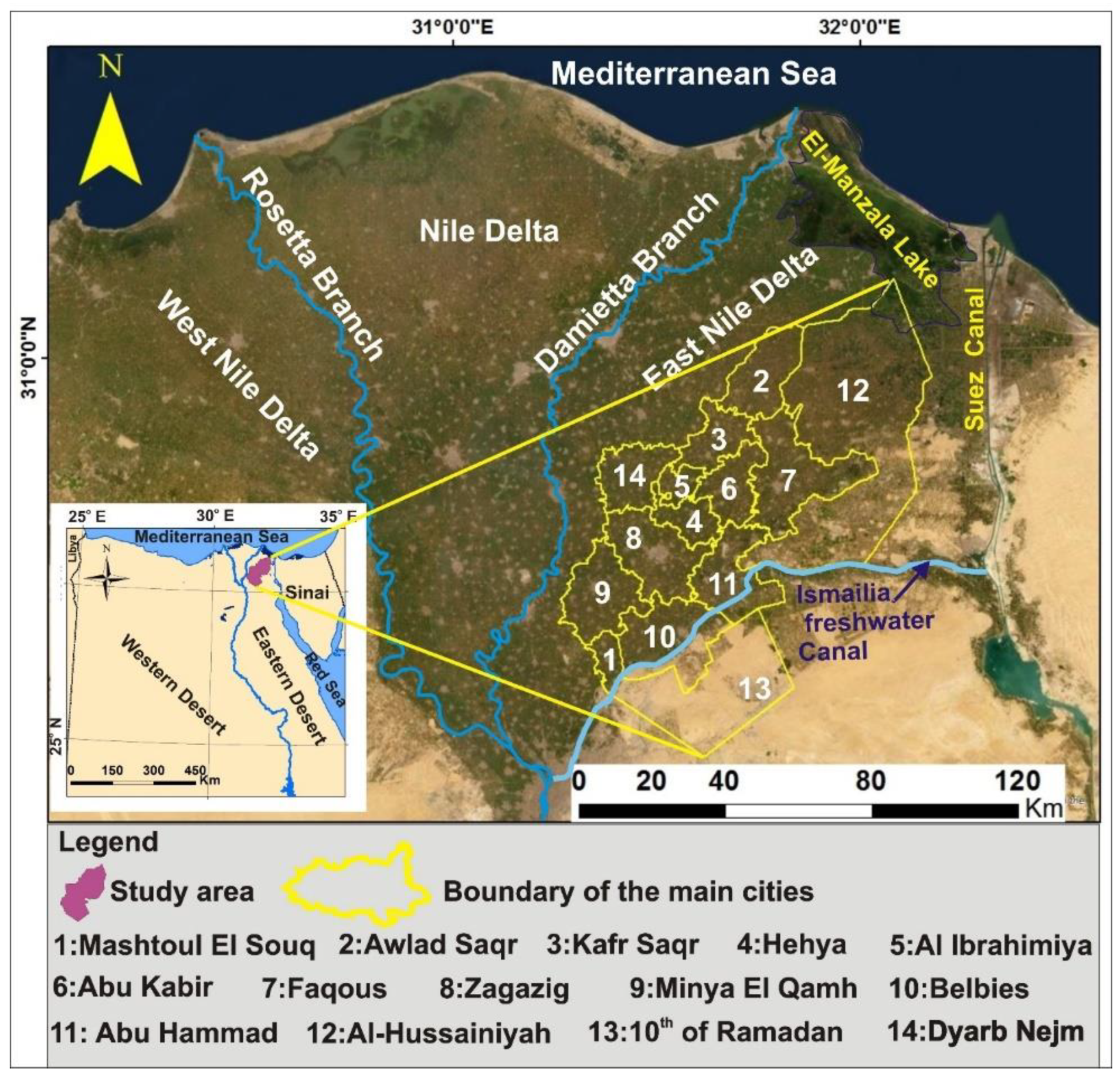
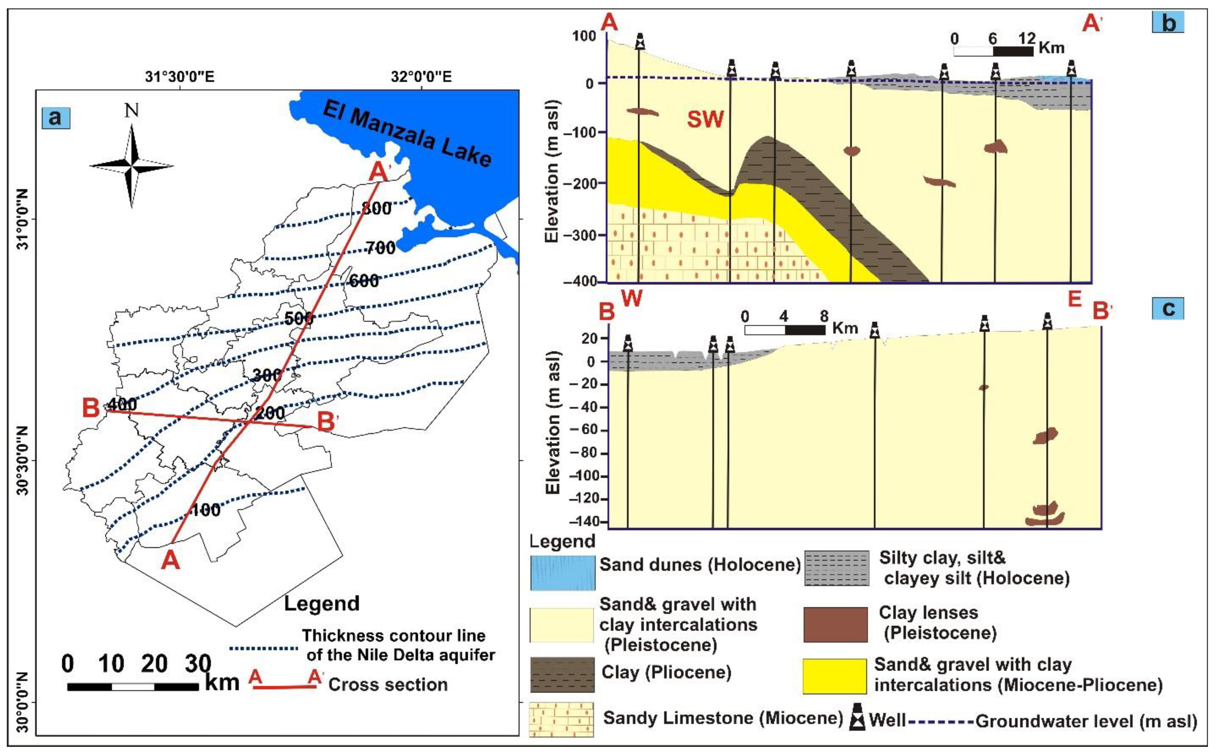
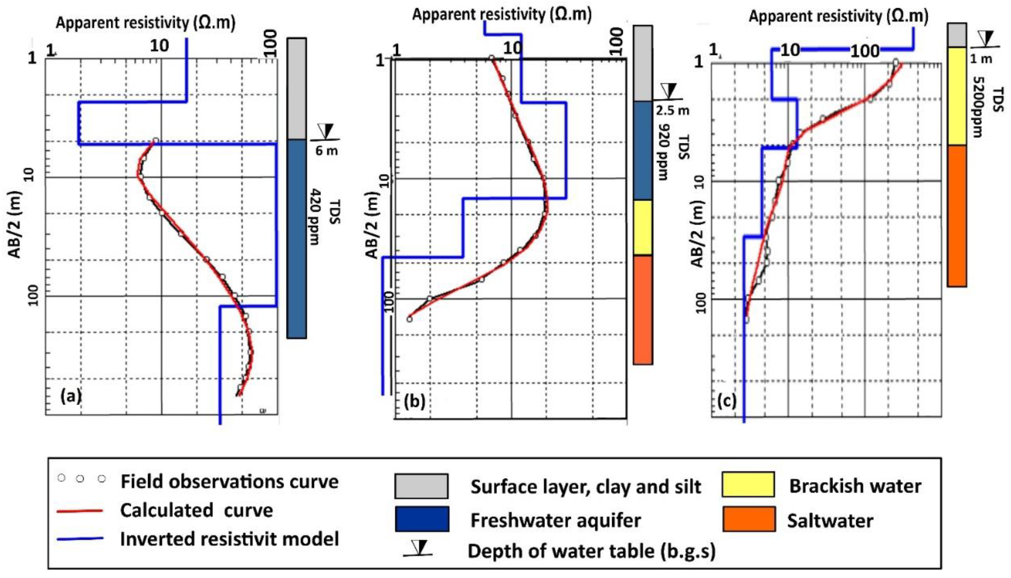
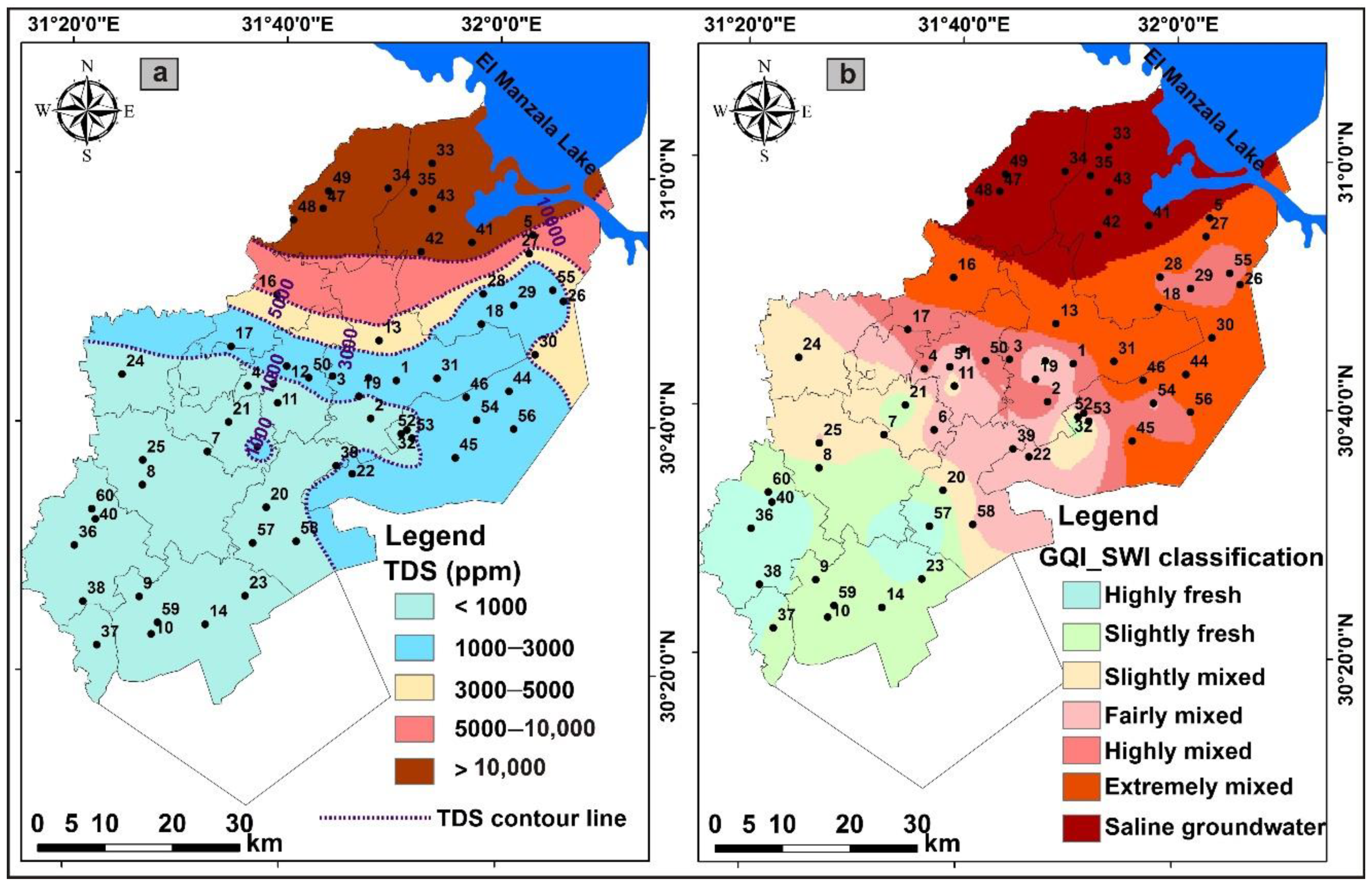
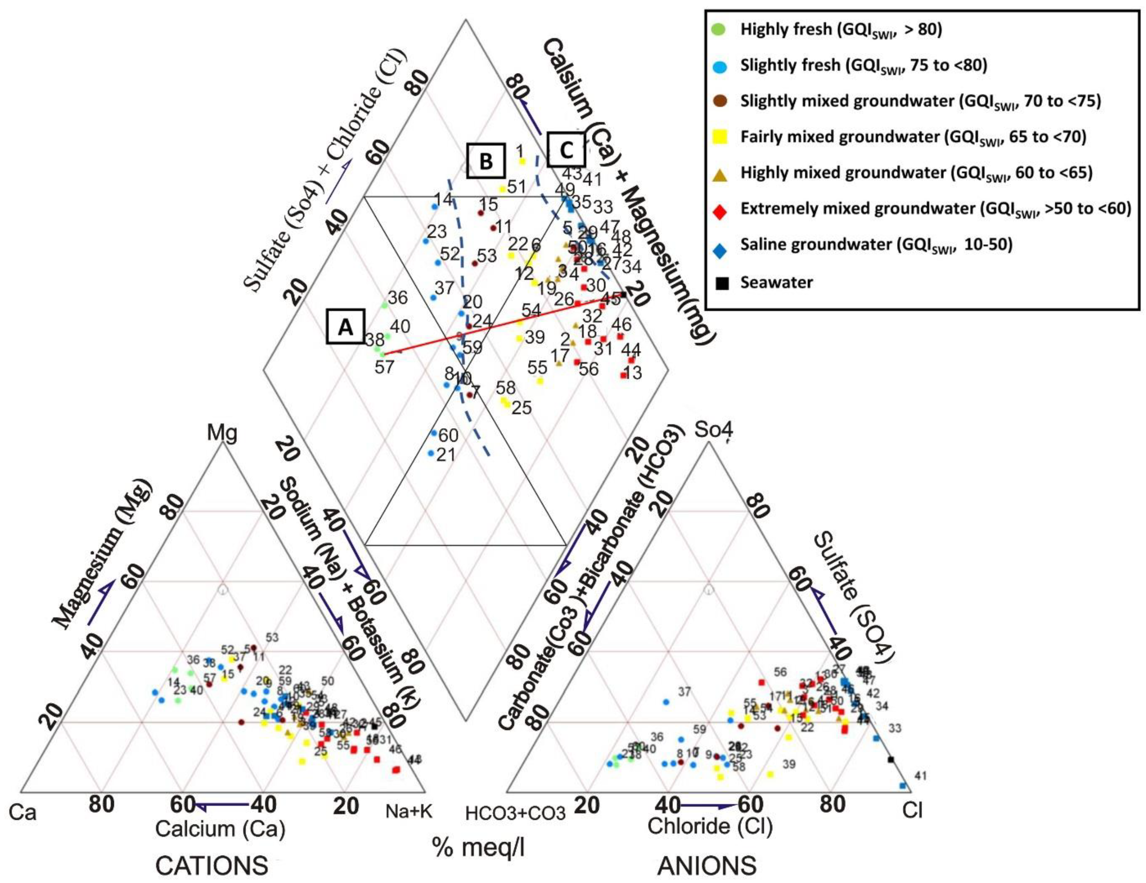
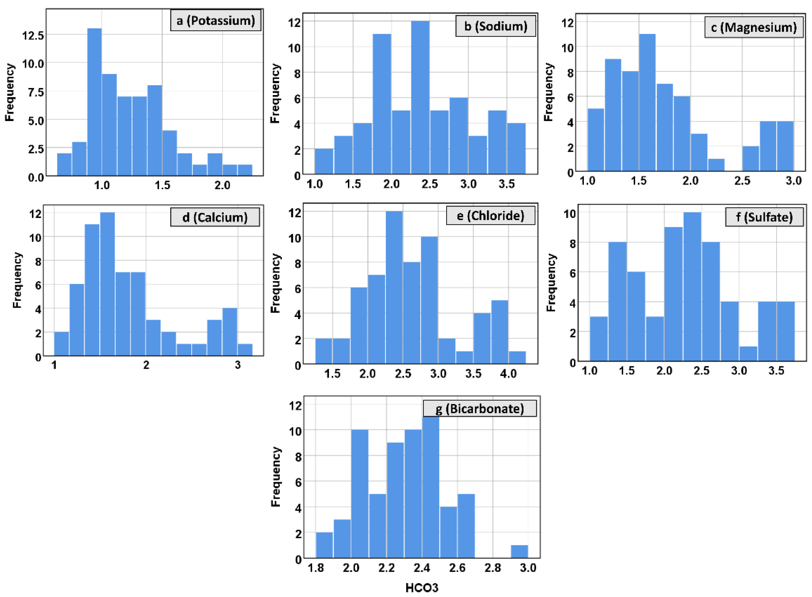
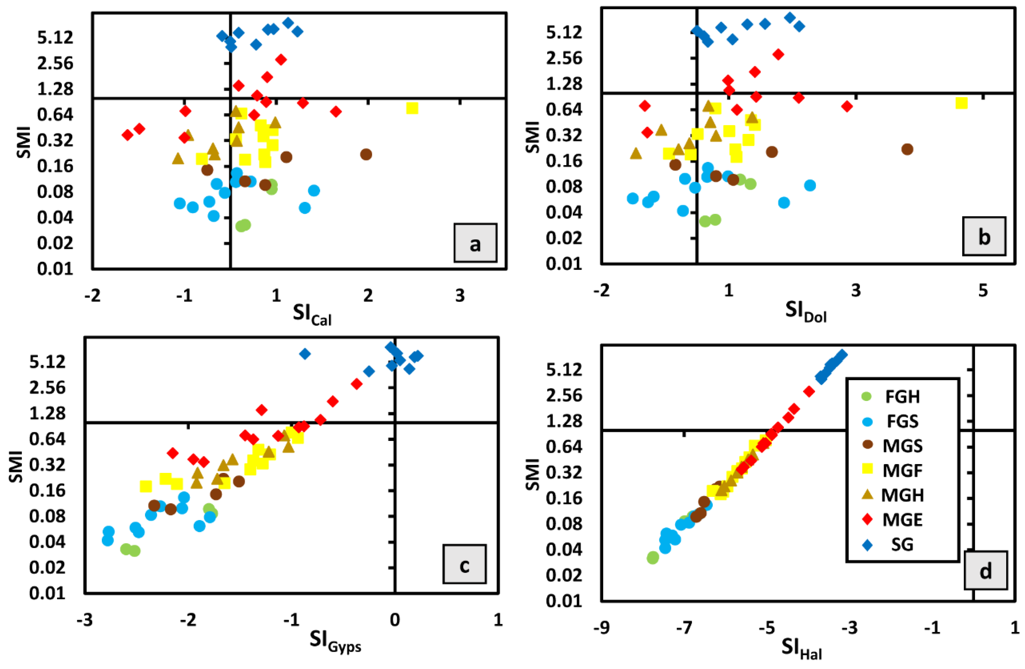
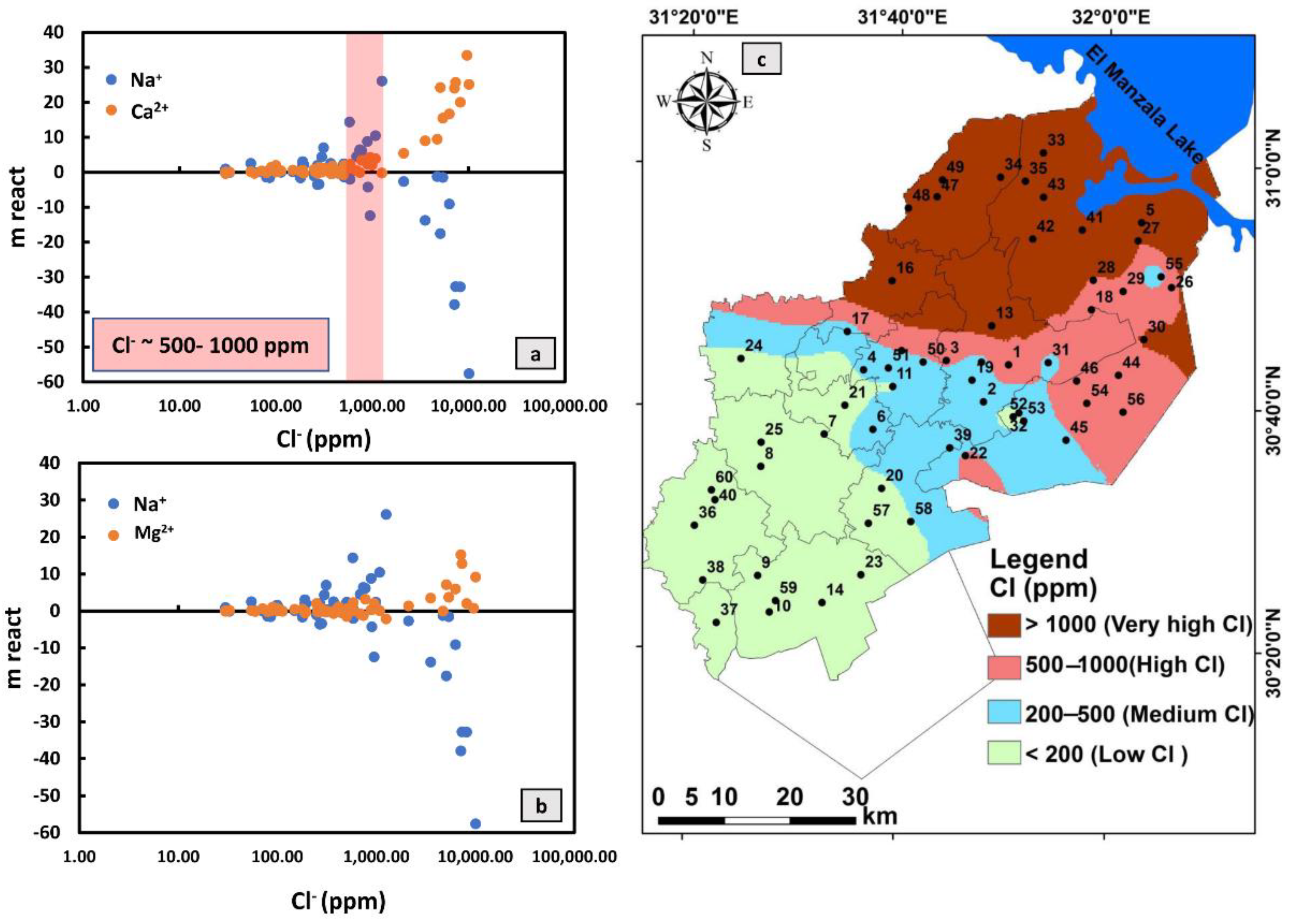
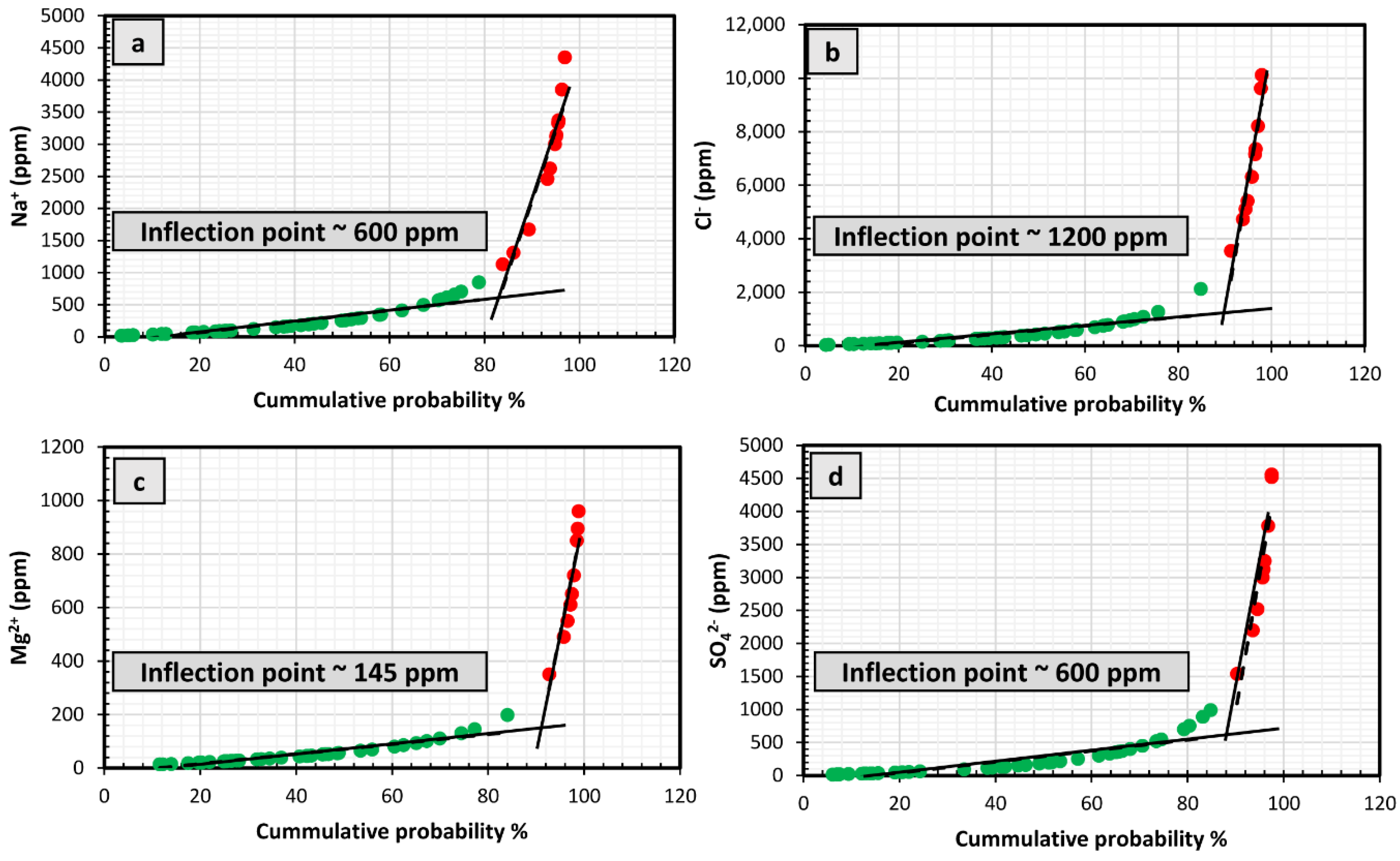
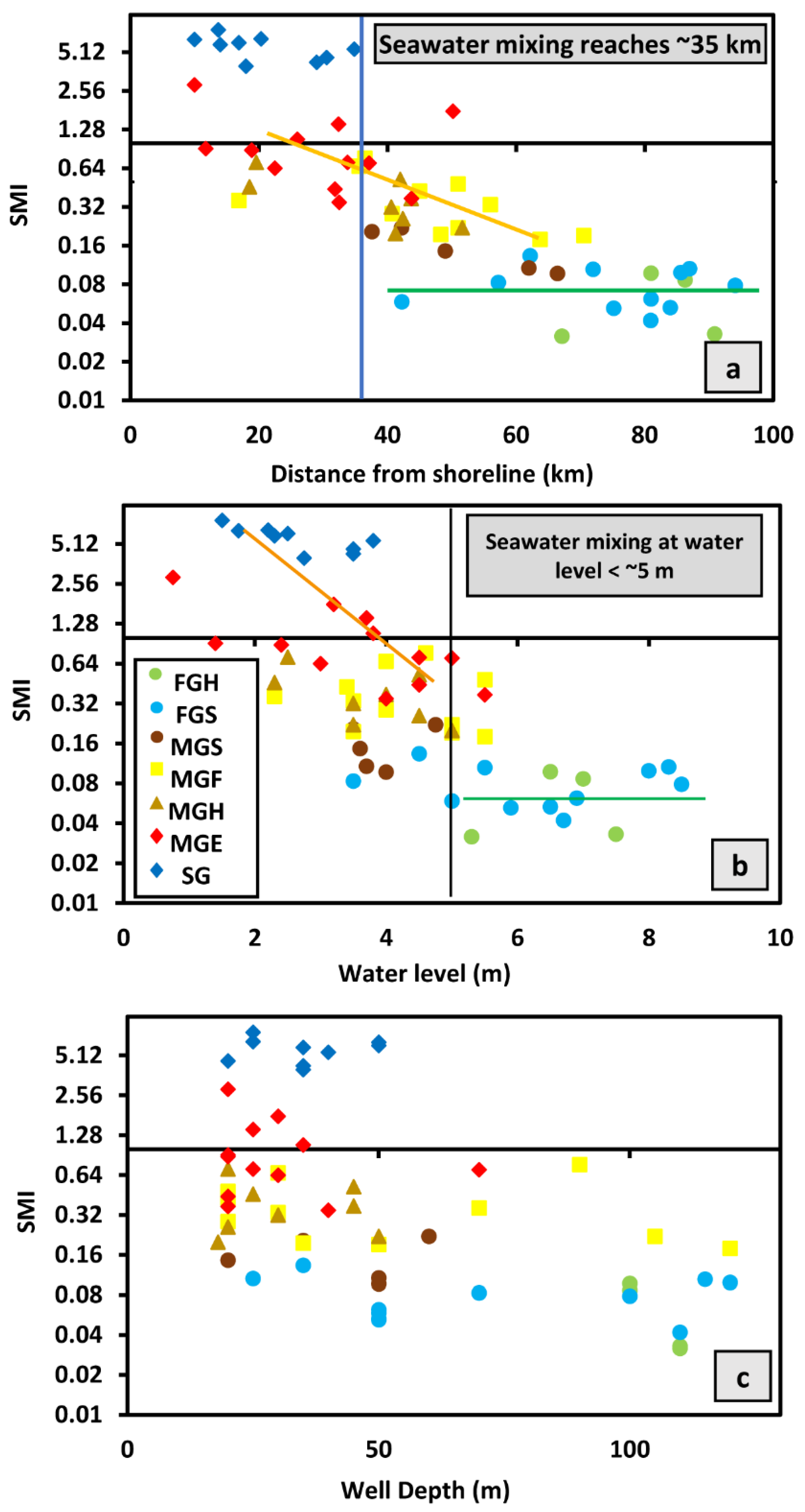
Table 1.
Descriptive statistics and coefficient of variation (CV) of hydrogeochemical data (concentrations unit is ppm; EC is in μS/cm).
Table 1.
Descriptive statistics and coefficient of variation (CV) of hydrogeochemical data (concentrations unit is ppm; EC is in μS/cm).
| Minimum | Maximum | Mean | Std. Deviation | CV% | |
|---|---|---|---|---|---|
| pH | 6.9 | 8.9 | 7.6 | 0.4 | 5 |
| TDS | 283 | 19550 | 3595 | 5397 | 150 |
| EC | 389 | 30030 | 5429 | 8135 | 150 |
| K+ | 4.5 | 146 | 24.3 | 26.5 | 109 |
| Na+ | 16 | 4350 | 734 | 1131 | 154 |
| Mg2+ | 13 | 960 | 146 | 242 | 166 |
| Ca2+ | 15 | 1554 | 227 | 366 | 161 |
| Cl− | 30 | 10120 | 1459 | 2557 | 175 |
| SO42− | 15 | 4560 | 654 | 1147 | 175 |
| HCO3− | 72 | 810 | 227 | 129 | 57 |
Table 2.
The Kaiser–Meyer–Olkin (KMO), Bartlett’s sphericity tests, and the factor analysis for the analyzed groundwater samples.
Table 2.
The Kaiser–Meyer–Olkin (KMO), Bartlett’s sphericity tests, and the factor analysis for the analyzed groundwater samples.
| Kaiser–Meyer–Olkin Measure of Sampling Adequacy | 0.79 | |||
| Bartlett’s Test of Sphericity | Approx. Chi-Square | 2604.09 | ||
| df | 153 | |||
| Sig. | 0.000 | |||
| Rotation Sums of Squared Loadings | Total | 8.96 | 3.41 | 3.11 |
| % of Variance | 49.78 | 18.95 | 17.29 | |
| Cumulative % | 49.78 | 68.72 | 86.02 | |
| 1 | 2 | 3 | ||
| EC | 0.97 | 0.22 | −0.01 | |
| TDS | 0.97 | 0.22 | −0.02 | |
| Mg | 0.97 | 0.16 | −0.01 | |
| Cl | 0.95 | 0.21 | −0.04 | |
| Na | 0.95 | 0.26 | −0.02 | |
| Ca | 0.95 | 0.15 | −0.02 | |
| SO4 | 0.89 | 0.21 | −0.05 | |
| SI Gypsum | 0.75 | 0.54 | 0.12 | |
| SI Halite | 0.73 | 0.62 | 0.05 | |
| K | 0.73 | 0.19 | 0.19 | |
| SAR | 0.69 | 0.51 | −0.02 | |
| Distance | −0.40 | −0.85 | −0.08 | |
| Total Depth | −0.05 | −0.83 | 0.26 | |
| Water level | −0.35 | −0.83 | −0.11 | |
| SI Dolomite | 0.22 | 0.05 | 0.96 | |
| SI Calcite | 0.19 | 0.00 | 0.96 | |
| HCO3 | −0.08 | 0.02 | 0.81 | |
| pH | −0.40 | −0.16 | 0.69 | |
Publisher’s Note: MDPI stays neutral with regard to jurisdictional claims in published maps and institutional affiliations. |
© 2022 by the authors. Licensee MDPI, Basel, Switzerland. This article is an open access article distributed under the terms and conditions of the Creative Commons Attribution (CC BY) license (https://creativecommons.org/licenses/by/4.0/).
Share and Cite
MDPI and ACS Style
Abu Salem, H.S.; Gemail, K.S.; Junakova, N.; Ibrahim, A.; Nosair, A.M. An Integrated Approach for Deciphering Hydrogeochemical Processes during Seawater Intrusion in Coastal Aquifers. Water 2022, 14, 1165. https://doi.org/10.3390/w14071165
AMA Style
Abu Salem HS, Gemail KS, Junakova N, Ibrahim A, Nosair AM. An Integrated Approach for Deciphering Hydrogeochemical Processes during Seawater Intrusion in Coastal Aquifers. Water. 2022; 14(7):1165. https://doi.org/10.3390/w14071165
Chicago/Turabian StyleAbu Salem, Hend S., Khaled S. Gemail, Natalia Junakova, Amin Ibrahim, and Ahmed M. Nosair. 2022. "An Integrated Approach for Deciphering Hydrogeochemical Processes during Seawater Intrusion in Coastal Aquifers" Water 14, no. 7: 1165. https://doi.org/10.3390/w14071165
Note that from the first issue of 2016, this journal uses article numbers instead of page numbers. See further details here.