
An Operational Model for Remote Estimating Absorption of Optical Activity Constituents
by
Zhifeng Yu
1, 
Shoujing Yin
2,3,*,
Xiaohong Yuan
1,4,
Yaming Zhou
2,3,
Nan Wang
2,3,
Bin Meng
2,3 and
Bin Zhou
1,4,* 1
Institute of Remote Sensing and Earth Sciences, School of Information Science and Engineering, Hangzhou Normal University, Hangzhou 311121, China
2
Satellite Application Center for Ecology and Environment, Ministry of Ecology and Environment, Beijing 100094, China
3
State Environment Protection Key Laboratory of Satellite Remote Sensing, Beijing 100094, China
4
Zhejiang Provincial Key Laboratory of Urban Wetlands and Regional Change, Hangzhou 311121, China
*
Authors to whom correspondence should be addressed.
Water 2022, 14(7), 1154; https://doi.org/10.3390/w14071154
Submission received: 10 February 2022
/
Revised: 24 March 2022
/
Accepted: 30 March 2022
/
Published: 3 April 2022
(This article belongs to the Special Issue Application of Remote Sensing in Process Analysis and Lake-Wetland-Watershed Ecosystem)
Abstract
:The need for an accurate model that can derive the absorption coefficient of optical activity constituents from both marine water and coastal water remains necessary. This study aimed to develop an algorithm for determining the absorption coefficients for both phytoplankton and non-phytoplankton pigments [aph(λ) and adg(λ), respectively]. This algorithm included two portions: (1) the total absorption coefficients at the blue and green bands were computed using a neural network technology-based, quasi-analytical algorithm; and (2) the relationship between the adg(λ) coefficient and the coefficient of total absorption was analyzed. This algorithm was evaluated with both in-situ observations and remote-sensed satellite data. The results showed that the algorithm could produce acceptable results in the retrievals of adg(λ) and aph(λ) in both turbid and clear waters. The results also indicated that the proposed algorithm was effective for distinguishing between adg(λ) and aph(λ) from the total coefficients of absorption, even though more independent assessments using in-situ and remote-sensed data are required to further improve the approach.
1. Introduction
Optical properties have been broadly employed in marine environment protection and monitoring programs since these characteristics can be transformed to the concentrations of optically active components [1,2]. The coefficient of total absorption (a(λ)) is one of these optical properties. It has had a significant role in global energy budget estimations and in debates regarding global climate change. Generally, a(λ) in the visible regions is not only a product of the optical activity of pigments of phytoplankton (aph(λ)), but also dependent on non-phytoplankton pigments, including detritus and colored dissolved organic matter (CDOM). Similarity in spectral shapes has increased the complexity of spectrally identifying CDOM absorption, detritus absorption, and CDOM absorption with MODIS channels [3,4]. Therefore, CDOM absorption is usually combined operationally with detritus absorption, and both the CDOM absorption and detritus absorption are represented by adg(λ). Provided that the a(λ) values are known at two or more bands, the a(λ) can be partitioned into aph(λ) and adg(λ) [4,5].
Methods that are able to accurately infer information of aph(λ) and adg(λ) have been investigated over the last few decades, ranging from empirical to analytical methods. Simple or multiple regressions area applied to the desired absorption coefficients and spectral-ratio algorithms within empirical models [6,7]. Additionally, the aforementioned models can be employed to efficiently analyze remote-sensed data. However, some challenges have emerged when these methods have been applied to coastal and marine waters globally. For example, when the empirical absorption model put forward by Barnard et al. [8] was utilized to process the remote-sensed reflectance in the existing datasets, the values of a(490) were found to be significantly overestimated for a(490) < 0.038 m−1. However, these values were clearly underestimated for a (490) > 0.203 m−1. Previous analytical approaches have alternatively employed radiative transfer theories to simulate the reflectance within the highest part of the atmosphere with different atmospheric conditions and inherent optical characteristics [9]. However, such models need accurate profile information on the bio-optical characteristics of the water and atmosphere, which is sometimes difficult to get hold of for remote-sensed marine color. However, it was determined that these models could provide accurate absorption coefficients in water bodies with wide optical ranges.
Semi-analytical methods are promising techniques for portioning the absorption coefficients of optical activity constituents from the total absorption coefficients by means of assimilating certain analytical models into the absorption retrieval model using empirical functions [10]. Although considerable attention has been given to the construction and development of semi-analytical models for absorption coefficient separation, there remains an important requirement for developing a precise mathematical representation of both coastal and marine waters since emulation methods developed to date essentially remain applicable to regional coastal zones or open oceans only. As an example, when the QAA (quasi-analytical algorithm) [5] was selected to approximate the coefficients of absorptions from coastal waters with high turbidity, the total absorption coefficients were determined to be significantly underestimated since the QAA model could suppress the backscattering impacts on the total absorption retrieval instead of eradicating it [11]. This suppression may have yielded negative aph(λ) in waters of the Arctic, as well as for multiple coastal areas [12]. While the four-band model according to a neural network by Chen et al. [11] displayed the potential to provide more accurate a(λ) than the QAA model for both coastal water and marine water, the retrieval precision of aph(λ) and adg(λ) depended not only on the performance of the a(λ) retrieval model but also the total absorption decomposition model. However, this study’s practical experiments indicated that the decomposition models [5,13] had difficulty decomposing coastal aph(λ) and adg(λ) from a(λ). This difficulty was attributed to the optical complexity of these waters.
To accurately estimate aph(λ) and adg(λ) for worldwide coastal and marine waters, a total absorption decomposition model that could achieve a higher precision is still wanted. The performances of the aph(λ) and adg(λ) models were expected to be improved if the empirical and semi-analytical approaches were combined. The present study retrieved aph(λ) and adg(λ) in two steps as follows. First, the total absorption coefficients at the blue and green bands were computed using a neural network quasi-analytical algorithm (NQAA) by Chen et al. [14]. Second, the relationships between adg(λ) and the total absorption coefficients were analyzed. Based on these analytical results, a new empirical total absorption decomposition algorithm (TAA) was established.
2. Materials and Methods
2.1. Datasets Used
In this research study, to assess the applicability of the TAA model in isolating the absorption of phytoplankton and non-phytoplankton from the NQAA model-derived a(λ) within both marine water and coastal water, five independent datasets (Table 1), consisting of concurrent observations of remote-sensed reflectance and inherent optical properties, were utilized. The first (IOCCG) set of data was simulated utilizing a widely used numerical script. Extensive field observations [10] were used to generate bio-optical conditions, which were input into the model. Global field measurements were used to compile the second dataset [the NASA Optical Marine Algorithm Dataset (NOMAD dataset)], which was obtained from the SeaWiFS Project of the National Aeronautics and Space Administration (NASA) [15]. Field measurements made within the West Florida Shelf (WFS), USA from 1999 to 2002 constituted the third dataset (WFS dataset). The fourth set of data was generated from observations of the silty coastal areas of the Yellow Sea and East China Sea in 2003 (YCE dataset). These four datasets were compiled by a range of studies in the US, Europe, and China using a variety of instruments. All of the measurements were closely monitored and followed processing and deployment protocols that were rigorous and community-defined [16]. These datasets were separated into two categories: (1) the NOMAD and IOCCG datasets were utilized for initialization of the model; (2) the YCE and WFS datasets were employed for model evaluation. The accuracy assessment of the satellite-derived absorption coefficients of optical activity constituents using the TAA model was determined to be a very interesting undertaking. Therefore, this study collected a synchronized dataset, which consisted of synchronized, satellite-observed, remote-sensed reflectance and field-measured coefficients of absorption, for a match-up analysis. This dataset was obtained from SeaBASS. Additionally, this study obtained 12 synchronized, satellite-observed, remote sensing reflectance and field-measured absorption coefficients from the East China and Yellow seas. These coefficients were added to the synchronized dataset.
2.2. Construction of the TAA Model
The total absorption minus water absorption (anw(λ)) could be expanded as follows:
The magnitudes and shape of aph(λ) were determined to be very variable due to the alterations in pigment composition and the effects of pigment packaging [3]. As a result, the spectral ratio of aph(λ) was highly variable with the phytoplankton size classes and chlorophyll-a concentrations. Fortunately, many previous studies have reported that the second-order quadratic formula could be used to link the relationship of aph(λ) between the blue bands and 490 nm as follows:
where A0 and A1 represent the empirical coefficients that depend on the wavelength.
Generally, the CDOM absorption spectrum can be obtained using a simple single exponential model [9,17]:
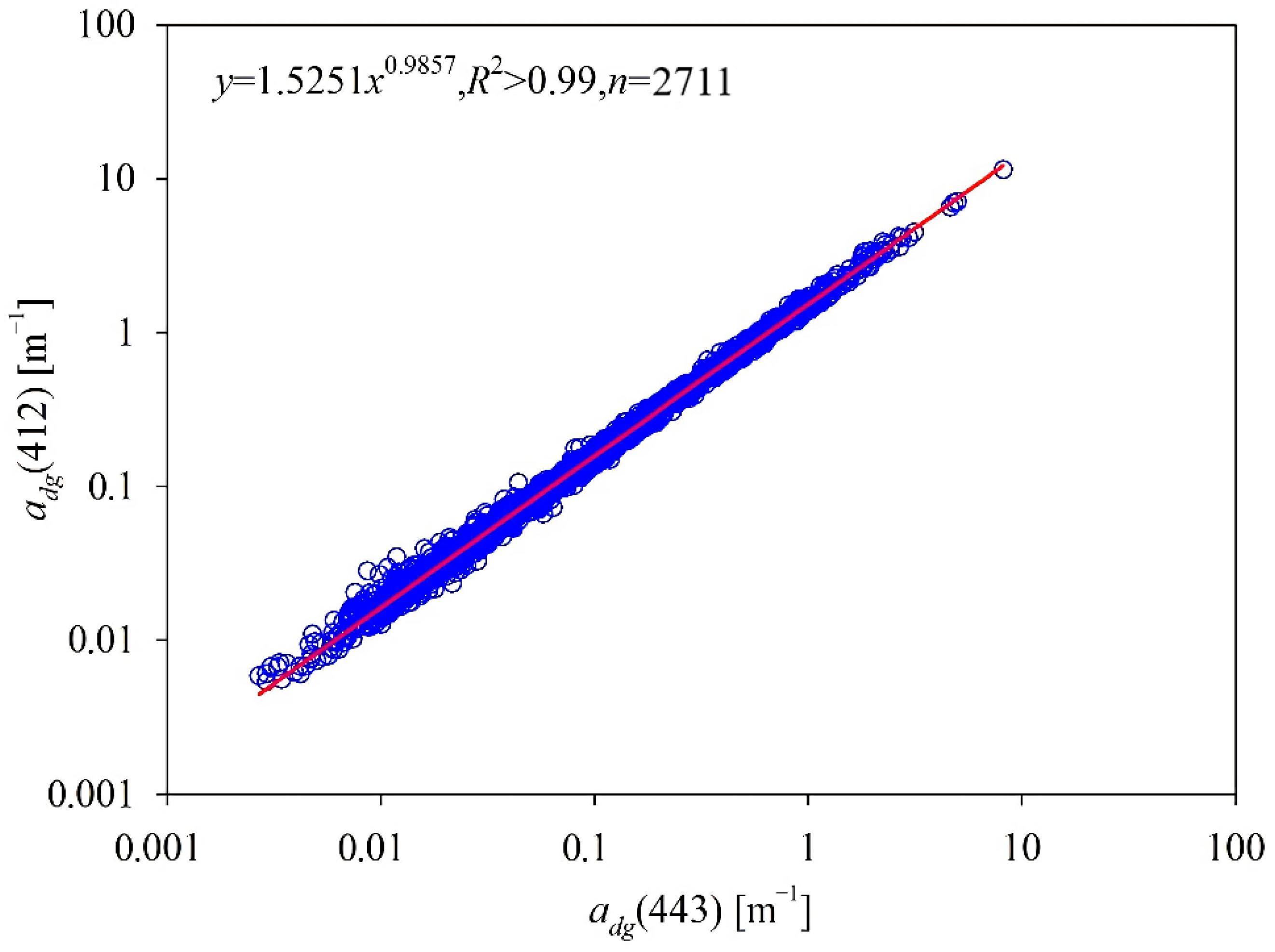
where S is the spectral slope coefficient of an exponent, which is applied to identify the absorption curve spectral shape. Based on the 2711 match-ups of adg(412) and adg(443) in this study’s dataset, adg(412) was exponentially dependent on adg(443), whose determination coefficient was >0.99 (Figure 1). By combining the formula in Figure 1 with Equation (3), the slope of the coefficient of absorption of the non-phytoplankton could be determined as follows:
By substituting Equations (2)–(4) in Equation (1) in the blue bands, adg (443) could be mathematically expressed as a function of anw (λ) in the three blue bands. In turbid and/or productive waters, the variations in the Rrs(λ) ratio are largely determined by the absorption of phytoplankton, detritus, and CDOM. In these types of waters, the CDOM, phytoplankton, there is such strong absorption of light by detritus that the signal leaving water in the blue regions is negligible [11]. Consequently, minor variations in the optical activity constituents may not alter reflectance at the blue wavelengths in waters with complex optical properties, which may inevitably impact the algorithm’s retrieval accuracy. Therefore, this study proposed deriving adg(443) product data using one model for turbid waters, while another different model would be employed for open oceans. These two models needed to be joined to produce smooth adg(443) data for both clear and turbid waters, and also for water areas with intermediate transparency. Therefore, the approach proposed by Wang et al. [18] was selected to account for this issue. A conceptual TAA model can be denoted as follows:
where f is an empirical function that can be determined using a regression analysis approach and J represents the red/blue ratio of Rrs(λ).
2.3. Accuracy Assessment
In this study, the MRE (mean relative error) and RMSE (root-mean-square error) were used to assess the precision of the absorption coefficient retrieval models. The RMSE was calculated using the following equation [10,19]:
where xmod,i represents the simulated ith element; xobs,i is the observed ith element; and N denotes the element total number. Traditionally, the MRE is typically evaluated using the formula (xmod,I − xobs,i)/xobs,i. However, the (xmod,i − xobs,i)/xobs,i ratio may become large when one dataset contains substantial errors. Therefore, biased estimates of relative difference are created. Consequently, an unbiased MRE was estimated using the following formula [20]:
3. Results
3.1. Model Initialization
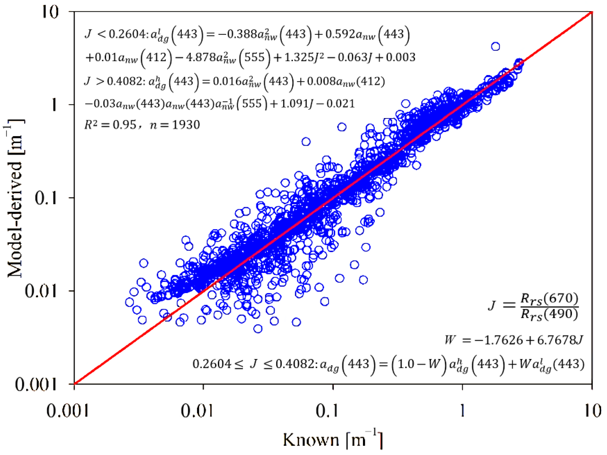
For prediction purposes, a large evaluation dataset (IOCCG and NOMAD datasets), which consisted of synchronized observations of the remote-sensed reflectance and inherent optical properties, was fed to run the NQAA model. To minimize the effects of some of the systematic uncertainty originating from the NQAA model on the adg(443) prediction, NQAA model-derived a(λ) data were utilized to determine the optimal function for the adg(443) retrieval. Based on the 1930 field measurements in the IOCCG and NOMAD datasets, the optimal TAA model was established as follows:
where l represents the low value and h represents the high value.
The results showed the optimal TAA model for adg(443) retrieval, whose maximum determination coefficient was 0.95, as detailed in Figure 2, that is, the TAA model was able to account for 95% of the variations in adg(443) in the initialization dataset. In this study, judging by the determination coefficient, the TAA model was determined to be an effective predictor of adg(443) using remote-sensed reflectance in waters with wide variations in optical conditions (Table 1). However, slight overestimations were still observed in the very small values (adg(443) < 0.01 m−1.
3.2. Model Evaluation
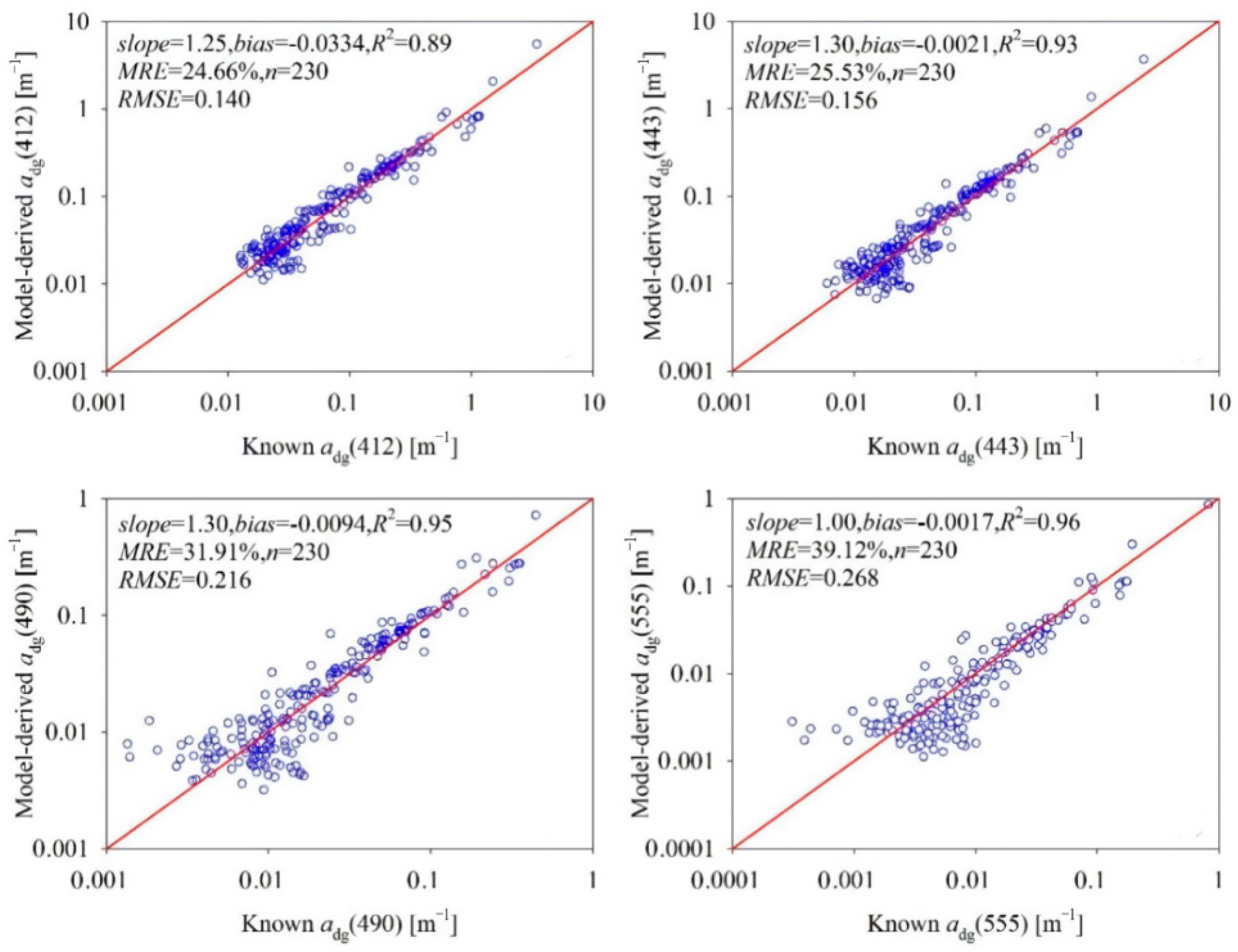
For this study’s model evaluation, the field-measured remote sensing reflectance of the WFS dataset was fed to the TAA model to derive adg(λ). The derived inherent optical characteristics were then related with the observed physical properties. The results of the performance of the model are shown in Figure 3. Based on 230 samples obtained from the WFS, the TAA model achieved good performance in separating adg(λ) from the NQAA model-derived a(λ) for the WFS, with a minimum determination coefficient of 0.89. The TAA model was able to account for more than 89% of the adg(λ) variations in the WFS. Moreover, as shown in Figure 3, the accuracy of the TAA model decreased with an increase in the increasing wavelength. For example, the MRE values had a significant wavelength-dependent feature according to the following order: 412 < 443 < 490 < 555 nm. These findings suggested that the TAA model effectively predicted adg(λ) using remote-sensed reflectance.
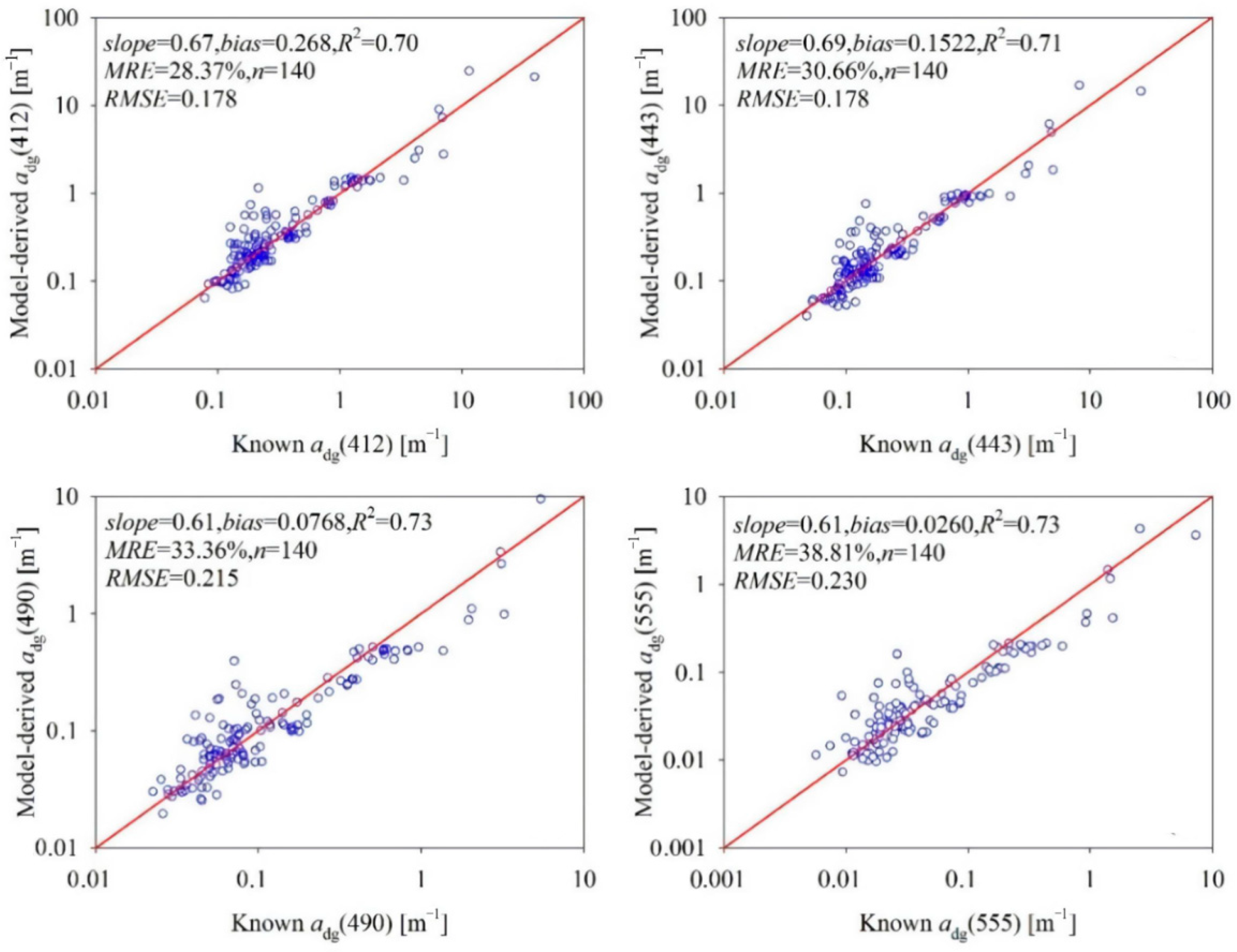
The performance and stability of the TAA model were further assessed using the independent YCE dataset. Figure 4 shows the accuracy evaluation of the TAA model in deriving adg(λ) from the Yellow and East China Seas datasets. It was found that the TAA model did not need additional optimization of the site-specific parameterization to accurately simulate the adg(λ) in water bodies with widely different bio-optical properties (Table 1). For example, for adg(443), which ranged from 0.048 to 8.168 m−1, the minimum coefficient of determination of the linear regression between the observed adg(λ) and model-derived adg(λ) was 0.70, while the corresponding MRE values did not exceed 38.81%. In contrast, the TAA model performances when applied to the Yellow and East China Seas were comparable to that for the WFS. Although the optical characteristics in the Chinese coastal zone were far more complex compared to those of the WFS (Table 1), the TAA model was still able to accurately predict adg(λ). The application of the TAA model to these two independent datasets yielded MRE values of the model-predicted variables of 26.06%, 27.47%, 32.46%, and 39% at 412, 443, 490, and 555 nm, respectively. It was therefore concluded that the TAA model can be applied to simulate adg(λ) for global coastal and marine waters.
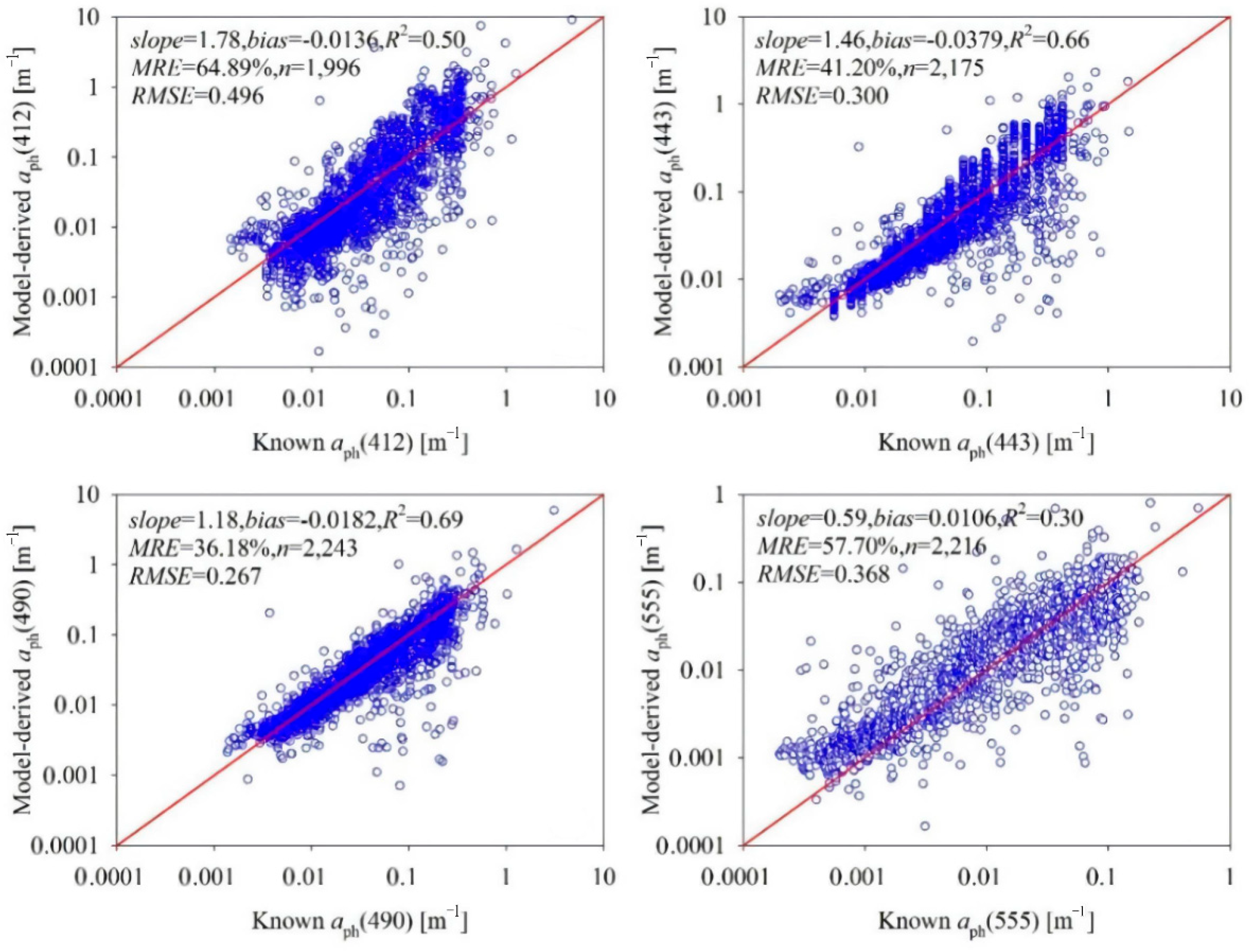
Provided that adg(λ) is known, aph(λ) can be easily determined using Equations (3) and (4). Figure 5 shows the precision of the TAA model in predicting aph(λ) from global coastal and marine waters. The results indicated that aph(λ) could be effectively derived from the total coefficient of absorption using the TAA model. For example, with aph(443) varying from 0.0002 to 1.457 m−1 in all four of the datasets, the scatter plots of simulated and observed aph(λ) were tightly concentrated around the 1:1 line. Application of the TAA model to all of the datasets yielded aph(λ) with an MRE value < 64.89% and an RMSE value < 0.497, as shown in Table 1. The accuracy of the TAA model was superior in estimating aph(λ) from adg(λ). When the NQAA model-derived a(λ0) incurred an error, a(λ) will also incur an error. Since adg(λ) is “fixed” with a high accuracy, the a(λ) error was propagated to aph(λ) since aph(λ) was calculated from a(λ) using Equation (5). Simultaneously fixing the accuracies of adg(λ) and aph(λ) was difficult unless the accuracy of a(λ) could first be fixed.
4. Discussion
4.1. Comparison with the QAA Model Performance
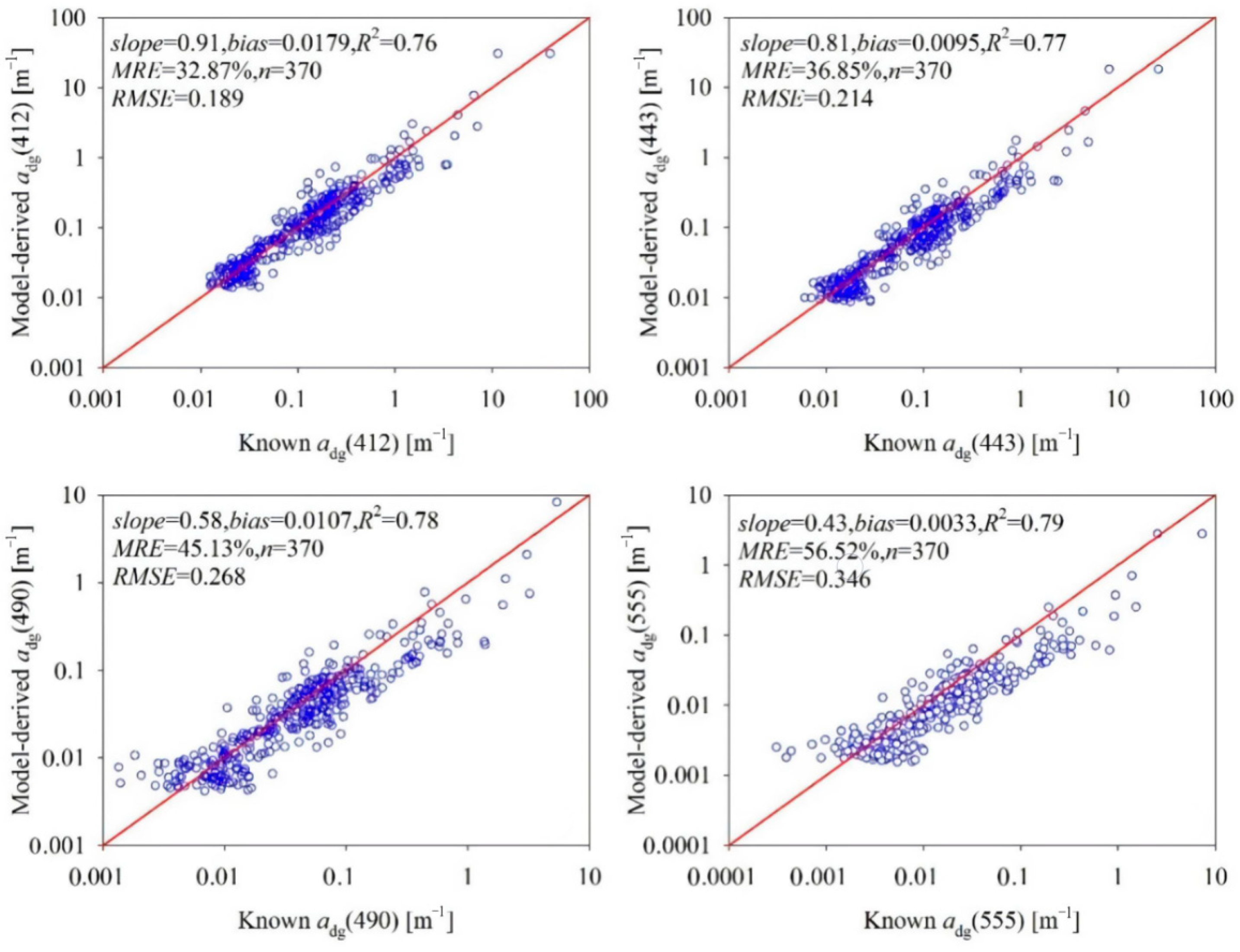
Various studies have previously described the QAA model in detail. This study further illuminated the stability and precision of the TAA model in distinguishing between adg(λ) and aph(λ) from a(λ) by evaluating the performance of the QAA model. The QAA model is applied globally and was initialized using global coastal and marine datasets, including the IOCCG and NOMAD [10,21]. As the IOCCG dataset [10] and Lee et al. [21,22] have demonstrated, the QAA model has been shown to be robust within its applied to most worldwide marine waters, and also certain coastal waters with high turbidity. Hense, the model coefficients were not modified according to the datasets of bio-optical information compiled in the current study. The model evaluation was according to a comparison between adg(λ) and aph(λ) simulated by the QAA model with the observations from the WFS, Yellow Sea, and East China Sea (Figure 6). Based on 370 samples for adg(443), which ranged from 0.008 to 8.168 m−1 in the two separate datasets, the RMSE and MRE values of adg(λ) exceeded 0.346 and 56.52%, respectively. Additionally, the slopes of the linear regressions between simulated adg(λ) and observed adg(λ) were determined to vary from 0.45 to 0.91 among the datasets, whereas the corresponding coefficients of determination ranged from 0.76 to 0.78. The best performance occurred at 412 nm (MRE = 32.87%), while the worst performance occurred at 555 nm (MRE = 56.52%). A comparison of the TAA and QAA models could be applied to decompose adg(λ) from the NQAA model-derived a(λ) in coastal and marine waters. However, the former displayed a better performance than the latter. The TAA model decreased by 6.81%, 9.38%, 12.67%, and 17.52% in comparison with the QAA model MRE values when simulating the adg(412), adg(443), adg(490), and adg(555), respectively, from this study’s datasets.
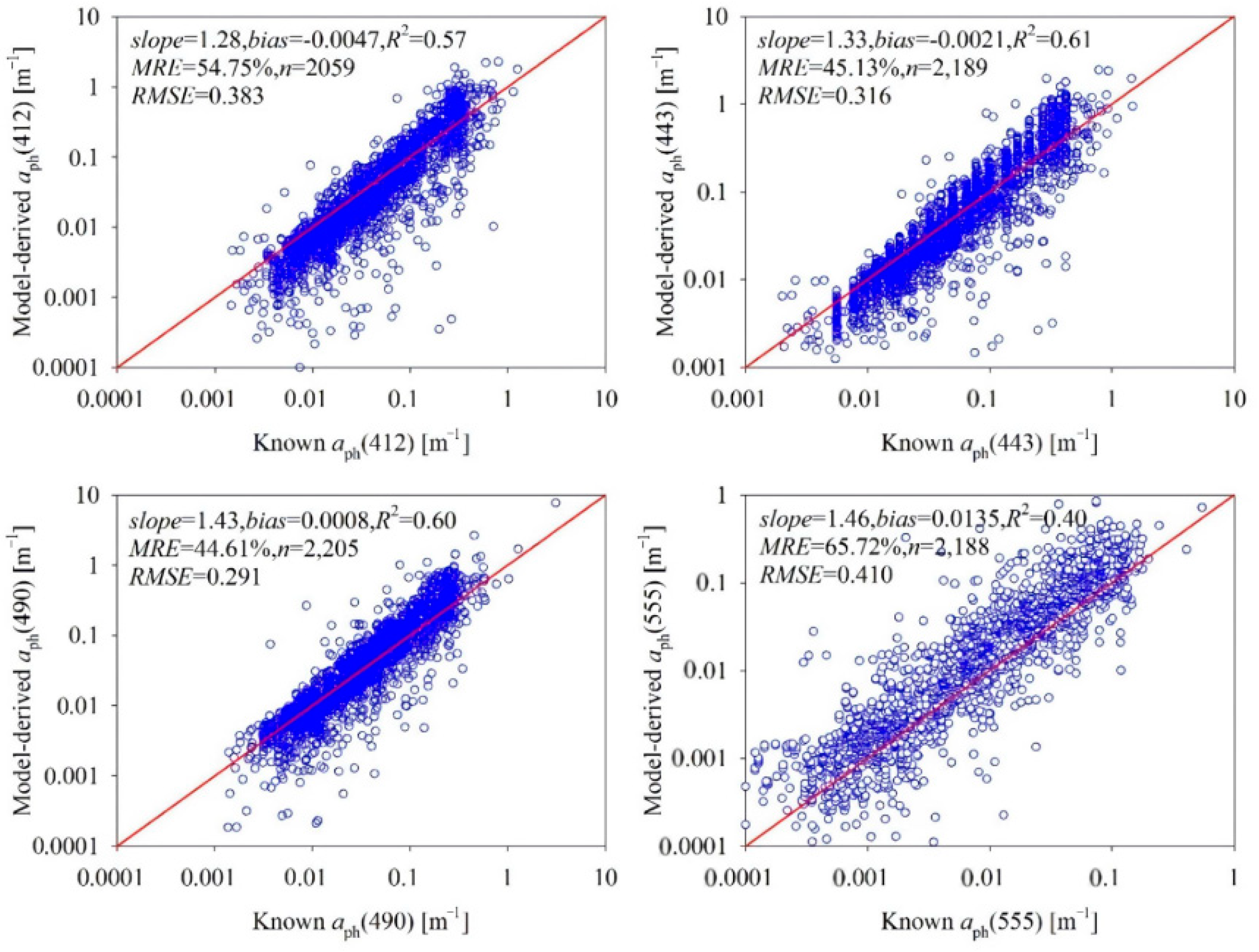
Figure 7 shows the accuracy evaluation of the QAA model in quantifying aph(λ) using the NQAA model-derived a(λ). Using the 2300 samples among the four datasets illustrated in Table 1, this study showed that the QAA model accurately predicted the aph(λ). With aph(443) varying from 0.0002 to 1.457 m−1, the scatter plots of the observed and model-derived aph(λ) were tightly concentrated around the 1:1 line, and the MRE values of the model-predicted variable did not exceed 65.72%. Therefore, based on this study’s dataset, and with the exception of 412 nm, the TAA model showed a better performance that the QAA model in estimating aph(λ) from the NQAA model-derived a(λ). Most importantly, the uncertainties in the QAA model-derived adg(λ) and aph(λ) were mainly generated from the following two steps: the total absorption coefficient retrieval procedures and the total absorption decomposition procedures [5]. Since the linear decomposition approach was able to allocate the NQAA model-derived a(λ) error into both adg(λ) and aph(λ), the accuracy of the QAA model-derived adg(λ) was similar to that of the QAA model-derived aph(λ), although the former was slightly better than the latter. This finding differed from that of the decomposition approach proposed by Lee et al. [5], in that the TAA model tried to fix the accuracy of adg(λ). Therefore, the NQAA model-derived a(λ) error was mainly propagated to aph(λ). As a result, compared with the QAA model, the improvement in the adg(λ) products using the TAA model was determined to be much more pronounced than that in the aph(λ) products in this study’s dataset.
4.2. Accuracy Evaluation of the Satellite-Derived Products
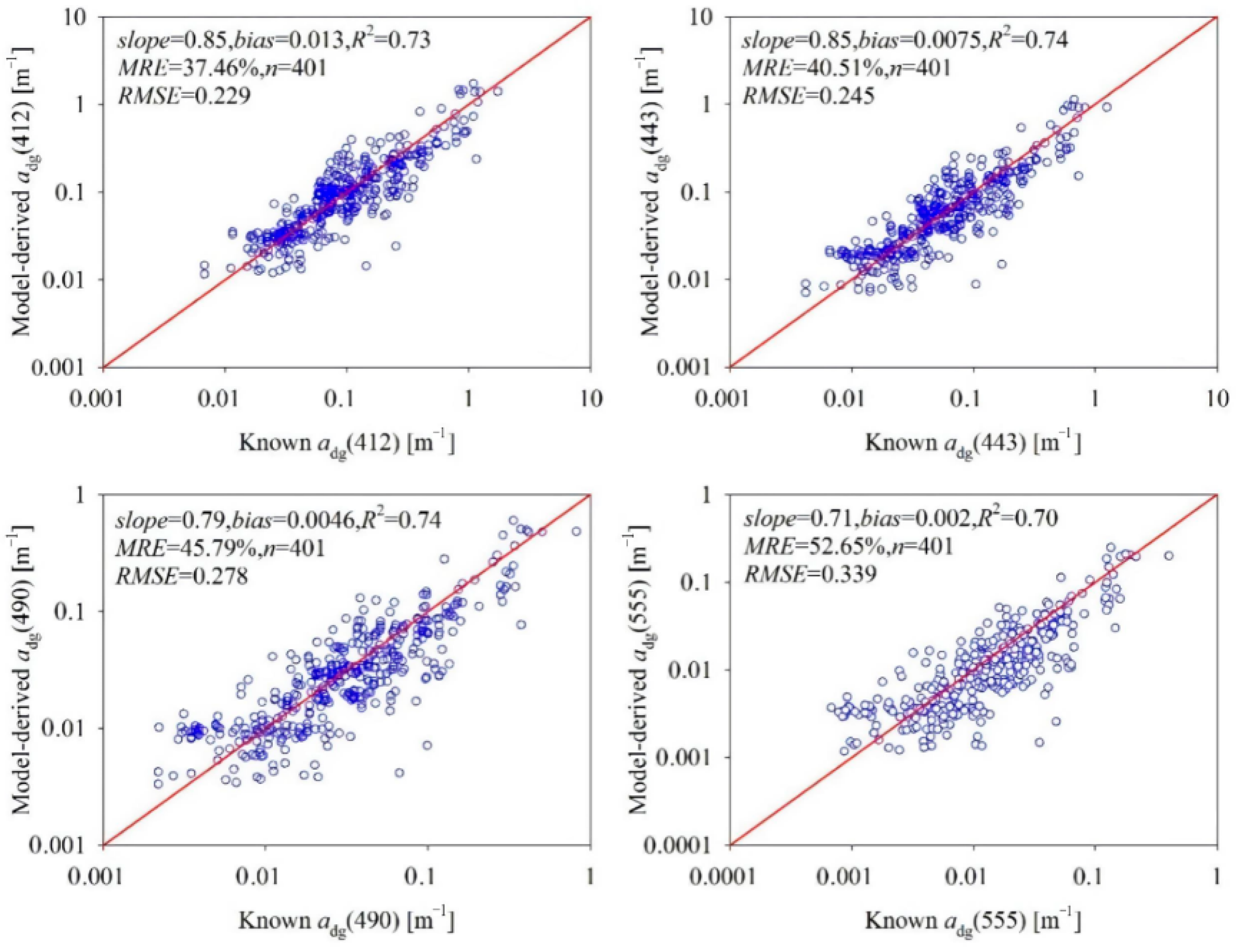
The TAA model-derived adg(λ) and aph(λ) were obtained from the satellite data following atmospheric correction. The accuracies of the adg(λ) and aph(λ) predicted from satellite data were evaluated comparing the quantified results with the observed results. The method of Bailey and Werdell [23] was applied to produce the adg(λ) and aph(λ) data predicted using satellite data, which were employed for the match analysis. As illustrated in Figure 8, the satellite-derived data are shown in comparison to the synchronized observed adg(λ), which had been obtained from global coastal and marine waters (Table 1). A comparison with the simulations of the TAA model with 401 field measurements showed that the model performance for retrieving adg(λ) from the satellite-derived remote sensing reflectance was good, in which the minimum determination coefficient was 0.7. The TAA model accounted for more than 70% of the variation in adg(λ) in the satellite-recorded signs. The MRE values varied from 37.46% to 52.65%, while the corresponding RMSE values changed from 0.229 to 0.339. These results implied that the TAA model was effective and could be successfully utilized to predict adg(λ) from satellite data in global coastal and marine waters.
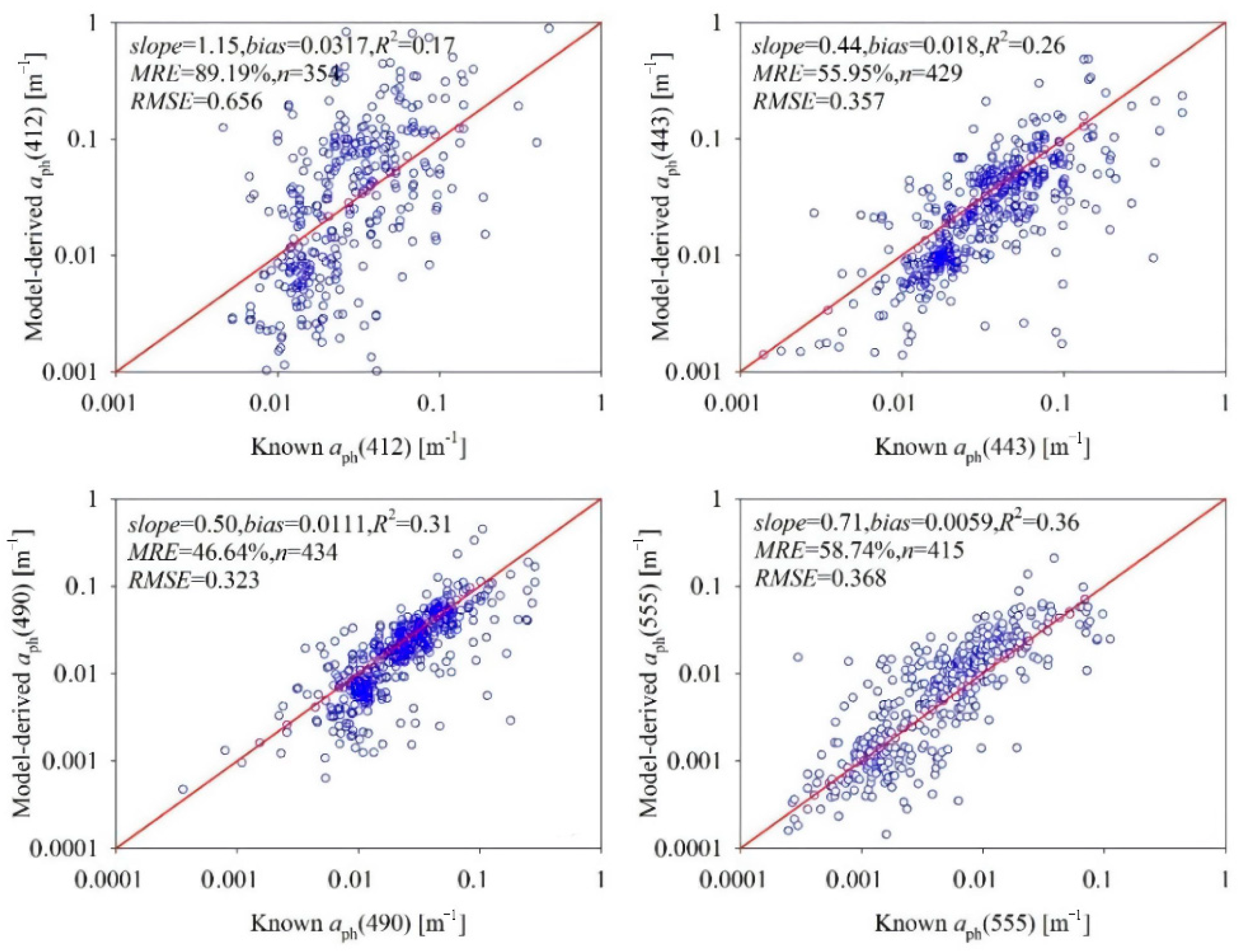
Figure 9 details the accuracies of the aph(λ) products derived from the AA model. Results implied that the TAA model could effectively predict aph(λ) in the blue and green bands with MRE values of 46.64 to 89.19%. Consistent with the results of Hu et al. [24], the residual error originating from the atmospheric correction enlarged with a decrease in the wavelength. These uncertainties inevitably influenced the output of the NQAA model. Chen et al. [14] proposed that since a(λ0) is “fixed” with high accuracy, the Rrs(λ0) error propagates to bb(λ0), where bb is the backscattering coefficient. Since bb(λ) is extrapolated from bb(λ0), some compensation will occur between bb(λ) and u(λ) for a(λ). Therefore, the NQAA model was able to suppress the influences of the residual error in the Rrs(λ) data in regards to the a(λ) retrieval instead of eradicating it. This suppression i exerted a residual influence on the accuracy of estimation of the TAA model-derived aph(λ). When adg(λ) was “fixed” with high accuracy, the majority of the NQAA model-derived a(λ) errors propagated to aph(λ). Consequently, the precision of the satellite-derived aph(λ) product was much poorer than that of adg(λ).
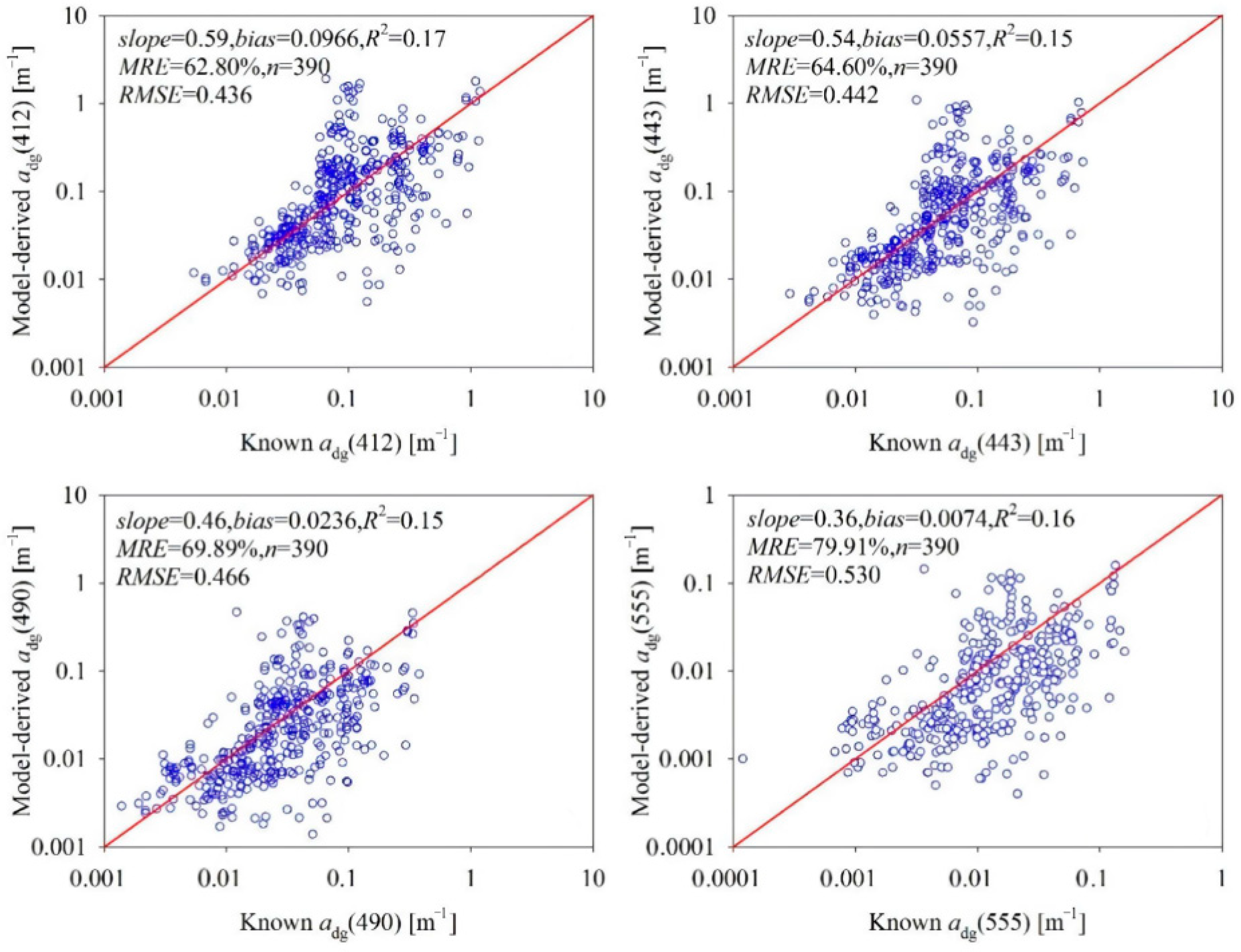
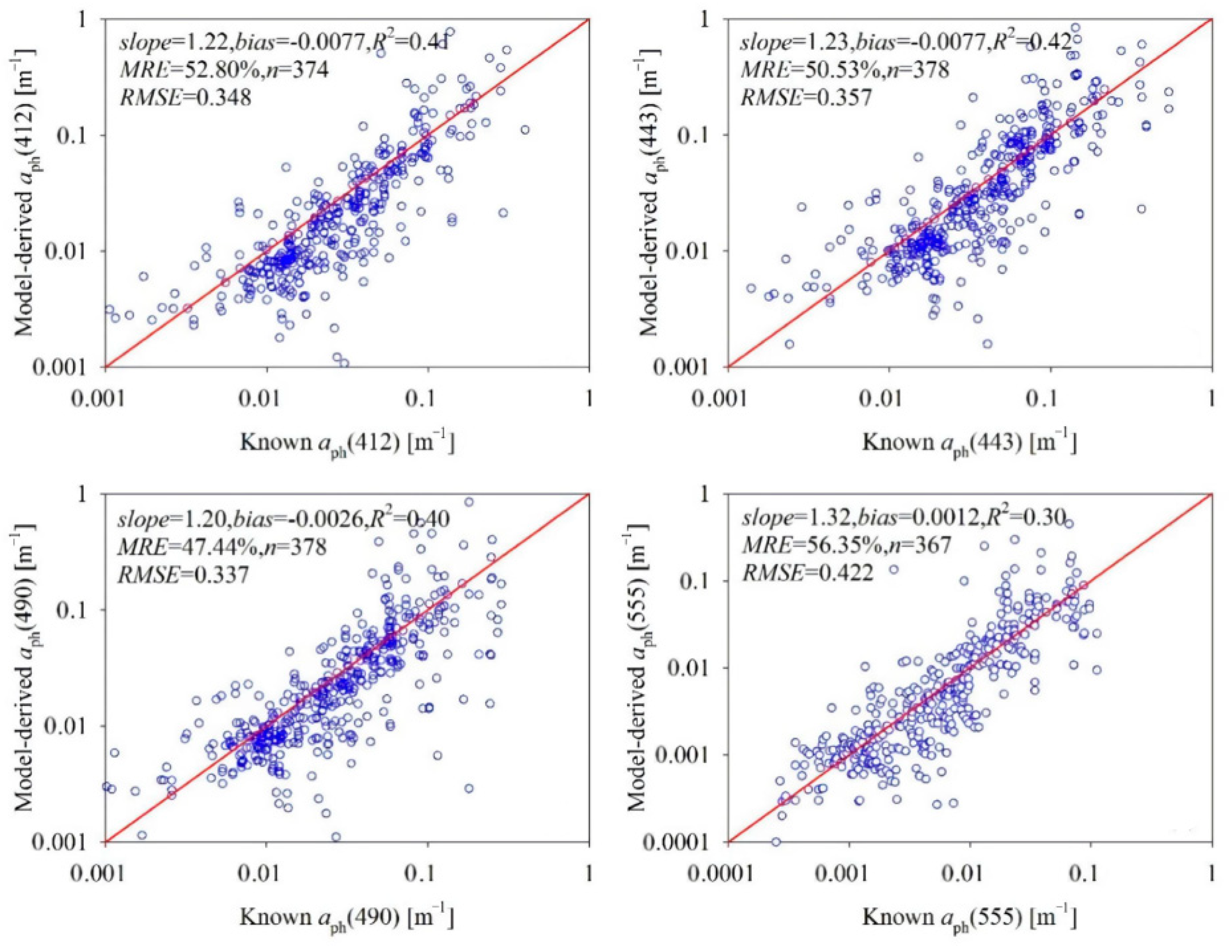
The generalized inherent optical property retrieval model (GIOP) resulted from two global, inherent, optical property algorithm workshops hosted by NASA as part of the Ocean Optics XIX and XX conferences [25]. To further illuminate the accuracy of the TAA model, this study presented the precision of the satellite-derived adg(λ) and aph(λ) utilizing the GIOP model. Figure 10 and Figure 11 show the performance of the GIOP model, which was assessed using the synchronized dataset detailed in Table 1. The TAA model performance was pronounced to be better than the GIOP model in the estimation of adg(λ). By using the satellite-derived, remote-sensed reflectance as the input, the TAA model was able to decrease the MRE values by >24% from the GIOP model when retrieving adg(λ) from global coastal and marine waters. On the other hand, besides for the 412 nm band, the TAA model produced a comparable performance with the GIOP model when predicting the aph(λ) from the satellite-observed remote sensing reflectance. These results confirmed that the TAA model did not need additional optimization of the site-specific parameterization to effectively generate the maps of adg(λ) and aph(λ) from the satellite data.
5. Conclusions
The present study proposed a TAA model to quantify adg(λ) and aph(λ) from remote-sensed and observed reflectances. The major differences between the present and previous studies are attributed to the notion that the TAA and NQAA combined model was able to directly predict the absorption related to phytoplankton and non-phytoplankton from the high spatial and temporal coverage of the satellite-provided, remote sensing reflectance. The data were prepared and assessed utilizing five separately simulated and observed datasets in global coastal and marine waters, and the TAA model showed acceptable accuracy in simulating adg(λ) and aph(λ) from this study’s dataset. Application of the TAA and QAA models to the data obtained from the WFS, Yellow Sea, and East China Sea showed that the performance of the TAA in the retrieval of adg(λ) was higher than that of the QAA model. Additionally, the TAA model generated a comparable accuracy to the QAA model in regard to the aph(λ) estimations. As adg(λ) had a fixed accuracy, the majority of the residual errors in the satellite-derived remote-sensed reflectance propagated to aph(λ). Consequently, the accuracy of the TAA model-derived aph(λ) was consistently poorer than the accuracy of the adg(λ) products.
Author Contributions
Conceptualization, Z.Y., S.Y. and B.M.; Data curation, S.Y., Y.Z. and N.W.; Investigation, N.W. and B.M.; Methodology, B.Z.; Writing—original draft, Z.Y., S.Y. and B.M.; Writing—review & editing, X.Y. and B.Z. All authors have read and agreed to the published version of the manuscript.
Funding
This research was funded by the National Key Research and Development Program of China (grant number 2021YFB3901101 and grant number 2017YFB0503902), the High Resolution Earth Observation Systems of National Science and Technology Major Projects (grant number 41-Y20A31-9003-15/17), and the Hangzhou Science and Technology Plan Guidance Project (grant number 20201231Y071).
Institutional Review Board Statement
Not applicable.
Informed Consent Statement
Not applicable.
Data Availability Statement
Not applicable.
Acknowledgments
The authors would like to thank NASA for their help in providing the NOMAD and IOCCG datasets, and thank all the reviewers who participated in the review.
Conflicts of Interest
The authors declare no conflict of interest.
References
- Chen, J.; He, X.; Liu, Z.; Xu, N.; Ma, L.; Xing, Q.; Hu, X.; Pan, D. An approach to cross-calibrating multi-mission satellite data for the open ocean. Remote Sens. Environ. 2020, 246, 111895. [Google Scholar] [CrossRef]
- Chen, J.; He, X.; Xing, X.; Xing, Q.; Liu, Z.; Pan, D. An Inherent Optical Properties Data Processing System for Achieving Consistent Ocean Color Products from Different Ocean Color Satellites. J. Geophys. Res. Ocean. 2019, 125, e2019JC015811. [Google Scholar] [CrossRef]
- Carder, K.L.; Chen, F.R.; Lee, Z.P.; Hawes, S.K.; Cannizzaro, J.P. MODIS Ocean Science Team: Algorithm Theoretical Basis Document. ATBD 19 Case 2 Chlorophyll-a. 2003, Version 7. Available online: http://modis.gsfc.nasa.gov/data/atbd/atbd_mod19.pdf (accessed on 30 March 2022).
- Garver, S.A.; Siegel, D.A. Inherent optical property inversion of ocean color spectral and its biogeochemical interpretation. 1. time series from the Sargasso Sea. J. Geophys. Res. Ocean. 1997, 102, 18607–18625. [Google Scholar] [CrossRef]
- Lee, Z.P.; Carder, K.L.; Arnone, R. Deriving inherent optical properties from water color: A multi-band quasi-analytical algorithm for optically deep waters. Appl. Opt. 2002, 41, 5755–5772. [Google Scholar] [CrossRef] [PubMed]
- Doerffer, R.; Schiller, H. The MERIS Case 2 water algorithm. Int. J. Remote Sens. 2007, 28, 517–535. [Google Scholar] [CrossRef]
- Morel, A.; Maritorena, S. Bio-optical properties of oceanic waters: A reappraisal. J. Geophys. Res. Ocean. 2001, 106, 7163–7180. [Google Scholar] [CrossRef] [Green Version]
- Barnard, A.H.; Zaneveld, J.R.V.; Pegau, W.S. In situ determination of the remotely sensed reflectance and the absorption coefficient: Closure and inversion. Appl. Opt. 1999, 38, 5108–5117. [Google Scholar] [CrossRef] [PubMed]
- Mobley, C.D. Light and Water: Radiative Transfer in Natural Waters; Academic Press: New York, NY, USA, 1994. [Google Scholar]
- IOCCG. Remote sensing of inherent optical properties: Fundamentals, tests of algorithms, and applications. In Reports of the International Ocean Colour Coordinating Group No.5; IOCCG: Dartmouth, NS, Canada, 2006. [Google Scholar]
- Chen, J.; Cui, T.; Quan, W. A neural network-based four-band model for estimating the total absorption coefficients from the global oceanic and coastal waters. J. Geophys. Res. Ocean. 2015, 120, 36–49. [Google Scholar] [CrossRef]
- Zheng, G.; Stramski, D.; Reynolds, R.A. Evaluation of the QAA algorithm for estimating the inherent optical properties from remote sensing reflectance in Arctic waters. In Proceedings of the Ocean Sciences Meeting, Portland, OR, USA, 22–26 February 2010. [Google Scholar]
- Smyth, T.J.; Moore, G.F.; Hirata, T.; Aiken, J. Semi-analytical model for the derivation of ocean color inherent optical properties: Description, implementation, and performance assessment. Appl. Opt. 2006, 45, 8116–8132. [Google Scholar] [CrossRef] [PubMed]
- Chen, J.; Lee, Z.; Hu, C.; Wei, J. Improving satellite data products for open oceans with a scheme to correct the residual errors in remote sensing reflectance. J. Geophys. Res. Ocean. 2016, 121, 3866–3886. [Google Scholar] [CrossRef] [Green Version]
- Werdell, P.J.; Bailey, S.W. The SeaWiFS Bio-Optical Archive and Storage System (SeaBASS): Current Architecture and Implementation; Goddard Space Flight Center: Greenbelt, MD, USA, 2002. [Google Scholar]
- Werdel; Bailey, S.W. An improved bio-optical data set for ocean color algorithm development and satellite data product variation. Remote Sens. Environ. 2005, 98, 122–140. [Google Scholar] [CrossRef]
- Shanmugam, P. New models for retrieving and partitioning the colored dissolved organic matter in the global ocean: Implications for remote sensing. Remote Sens. Environ. 2011, 115, 1501–1521. [Google Scholar] [CrossRef]
- Wang, M.; Son, S.; Harding, L.W., Jr. Retrieval of diffuse attenuation coefficient in the Chesapeake Bay and turbid ocean regions for satellite ocean color applications. J. Geophys. Res. Ocean. 2009, 114, C10011. [Google Scholar] [CrossRef]
- Laws, E.A. Mathematical Methods for Oceanographers: An Introduction; John Wiley and Sons: New York, NY, USA, 1997. [Google Scholar]
- Hooker, S.B.; Lazin, G.; Zibordi, G.; McLean, S. An Evaluation of Above- and In-Water Methods for Determining Water-Leaving Radiances. J. Atmos. Ocean. Technol. 2002, 19, 486–515. [Google Scholar] [CrossRef]
- Lee, Z.; Hu, C.; Shang, S.; Du, K.; Lewis, M.; Arnone, R.; Brewin, R. Penetration of UV-visible solar radiation in the global oceans: Insights from ocean color remote sensing. J. Geophys. Res. Ocean. 2013, 118, 4241–4255. [Google Scholar] [CrossRef] [Green Version]
- Lee, Z.P.; Werdell, P.J.; Arnone, R. An Update of the Quasi-Analytical Algorithm (QAA_V5). IOCCG Software Report 2009. Available online: https://www.ioccg.org/groups/Software_OCA/QAA_v5.pdf (accessed on 30 March 2022).
- Bailey, S.W.; Werdell, P.J. A multi-sensor approach for the on-orbit validation of ocean color satellite data products. Remote Sens. Environ. 2006, 102, 12–23. [Google Scholar] [CrossRef]
- Hu, C.; Feng, L.; Lee, Z. Uncertainties of SeaWiFS and MODIS remote sensing reflectance: Implications from clear water measurements. Remote Sens. Environ. 2013, 133, 168–182. [Google Scholar] [CrossRef]
- Werdell, P.J.; Franz, B.A.; Bailey, S.; Feldman, G.C.; Boss, E.; Brando, V.; Dowell, M.; Hirata, T.; Lavender, S.; Lee, Z.; et al. Generalized ocean color inversion model for retrieving marine inherent optical properties. Appl. Opt. 2013, 52, 2019–2037. [Google Scholar] [CrossRef] [PubMed]
Figure 1.
Empirical relationship between adg(412) and adg(443).

Figure 2.
Optimal TAA model for adg(443) prediction initialized from the IOCCG and NOMAD datasets.

Figure 3.
Accuracy evaluation of TAA model adg(λ) retrieval in West Florida Shelf.

Figure 4.
Accuracy evaluation of the TAA model in adg(λ) retrieval in the Yellow Sea and East Sea of China.
Figure 4.
Accuracy evaluation of the TAA model in adg(λ) retrieval in the Yellow Sea and East Sea of China.

Figure 5.
Accuracy evaluation of the TAA model in aph(λ) retrieval in global coastal and marine waters.
Figure 5.
Accuracy evaluation of the TAA model in aph(λ) retrieval in global coastal and marine waters.

Figure 6.
Accuracy of the QAA model in simulating adg(λ) for the West Florida Shelf, Yellow Sea, and East Sea of China.
Figure 6.
Accuracy of the QAA model in simulating adg(λ) for the West Florida Shelf, Yellow Sea, and East Sea of China.

Figure 7.
Accuracy of the QAA model in deriving phytoplankton coefficients of absorption.

Figure 8.
Precision of satellite-derived adg(λ) products using the TAA model.

Figure 9.
Accuracies of TAA model-simulated aph(λ) produced using satellite data.

Figure 10.
Accuracy of the remote-sensed coefficient of absorption of non-phytoplankton using GIOP model.
Figure 10.
Accuracy of the remote-sensed coefficient of absorption of non-phytoplankton using GIOP model.

Figure 11.
Precision of the remote-sensed coefficient of absorption of phytoplankton utilizing the GIOP model.
Figure 11.
Precision of the remote-sensed coefficient of absorption of phytoplankton utilizing the GIOP model.


Table 1.
A statistical summary of observed a(λ) for the NOMAD, YCE, WFS, IOCCG, and Bohai datasets.
| Dataset | a(λ) | Min. | Max. | Median | Mean | SD |
|---|---|---|---|---|---|---|
| IOCCG dataset n = 1000 | aph(443) | 0.005 | 0.416 | 0.056 | 0.115 | 0.518 |
| adg(443) | 0.004 | 2.642 | 0.153 | 0.497 | 0.628 | |
| NOMAD dataset n = 930 | aph(443) | 0.002 | 1.457 | 0.033 | 0.059 | 0.089 |
| adg(443) | 0.003 | 0.902 | 0.044 | 0.087 | 0.126 | |
| WFS dataset n = 230 | aph(443) | 0.008 | 0.684 | 0.025 | 0.050 | 0.072 |
| adg(443) | 0.006 | 0.900 | 0.039 | 0.088 | 0.134 | |
| YCE dataset n = 140 | aph(443) | 0.009 | 0.680 | 0.081 | 0.680 | 0.102 |
| adg(443) | 0.048 | 8.168 | 0.147 | 0.359 | 0.824 | |
| Synchronized dataset n = 437 | aph(443) | 0.001 | 0.540 | 0.034 | 0.053 | 0.065 |
| adg(443) | 0.003 | 1.250 | 0.055 | 0.105 | 0.146 |
Publisher’s Note: MDPI stays neutral with regard to jurisdictional claims in published maps and institutional affiliations. |
© 2022 by the authors. Licensee MDPI, Basel, Switzerland. This article is an open access article distributed under the terms and conditions of the Creative Commons Attribution (CC BY) license (https://creativecommons.org/licenses/by/4.0/).
Share and Cite
MDPI and ACS Style
Yu, Z.; Yin, S.; Yuan, X.; Zhou, Y.; Wang, N.; Meng, B.; Zhou, B. An Operational Model for Remote Estimating Absorption of Optical Activity Constituents. Water 2022, 14, 1154. https://doi.org/10.3390/w14071154
AMA Style
Yu Z, Yin S, Yuan X, Zhou Y, Wang N, Meng B, Zhou B. An Operational Model for Remote Estimating Absorption of Optical Activity Constituents. Water. 2022; 14(7):1154. https://doi.org/10.3390/w14071154
Chicago/Turabian StyleYu, Zhifeng, Shoujing Yin, Xiaohong Yuan, Yaming Zhou, Nan Wang, Bin Meng, and Bin Zhou. 2022. "An Operational Model for Remote Estimating Absorption of Optical Activity Constituents" Water 14, no. 7: 1154. https://doi.org/10.3390/w14071154
Note that from the first issue of 2016, this journal uses article numbers instead of page numbers. See further details here.