
Flood Detection in Urban Areas Using Satellite Imagery and Machine Learning


1
iWERS Laboratory, Department of Civil and Environmental Engineering, University of South Carolina, Columbia, SC 29208, USA
2
Urban Water Group, San Diego State University, 5500 Campanile Dr., San Diego, CA 92182, USA
*
Author to whom correspondence should be addressed.
Water 2022, 14(7), 1140; https://doi.org/10.3390/w14071140
Submission received: 9 February 2022
/
Revised: 17 March 2022
/
Accepted: 23 March 2022
/
Published: 1 April 2022
(This article belongs to the Section New Sensors, New Technologies and Machine Learning in Water Sciences)
Abstract
:Urban flooding poses risks to the safety of drivers and pedestrians, and damages infrastructures and lifelines. It is important to accommodate cities and local agencies with enhanced rapid flood detection skills and tools to better understand how much flooding a region may experience at a certain period of time. This results in flood management orders being announced in a timely manner, allowing residents and drivers to preemptively avoid flooded areas. This research combines information received from ground observed data derived from road closure reports from the police department, with remotely sensed satellite imagery to develop and train machine-learning models for flood detection for the City of San Diego, CA, USA. For this purpose, flooding information are extracted from Sentinel 1 satellite imagery and fed into various supervised and unsupervised machine learning models, including Random Forest (RF), Support Vector Machine (SVM), and Maximum Likelihood Classifier (MLC), to detect flooded pixels in images and evaluate the performance of these ML models. Moreover, a new unsupervised machine learning framework is developed which works based on the change detection (CD) approach and combines the Otsu algorithm, fuzzy rules, and iso-clustering methods for urban flood detection. Results from the performance evaluation of RF, SVM, MLC and CD models show 0.53, 0.85, 0.75 and 0.81 precision measures, 0.9, 0.85, 0.85 and 0.9 for recall values, 0.67, 0.85, 0.79 and 0.85 for the F1-score, and 0.69, 0.87, 0.83 and 0.87 for the accuracy measure, respectively, for each model. In conclusion, the new unsupervised flood image classification and detection method offers better performance with the least required data and computational time for enhanced rapid flood mapping. This systematic approach will be potentially useful for other cities at risk of urban flooding, and hopefully for detecting nuisance floods, by using satellite images and reducing the flood risk of transportation design and urban infrastructure planning.
1. Introduction
Flooding poses a significant hazard to moving vehicles and causes traffic disruption by placing water flow in the transportation network, resulting in vehicles being swept away, injuries, and the loss of life of passengers. The remote detection of urban flooding over a large area will allow cities to develop flood maps to reduce risk during weather events. Mapping urban flood events is a challenge for three main reasons: the urban environment is highly complex with waterways at submeter resolutions, the flooding will be shallow and ephemeral, and ponding means that the flooding extent will be discontinuous. Hydrologic models that are the conventional approach in flood forecasting struggle with these factors, making the application of these techniques difficult. Attempts have been made to map urban flooding and flood risk with more traditional methods such as [1]. High resolution hydrologic models are effective at small scales (e.g., a few urban blocks) but the computational resources and highly accurate inputs required to properly model urban flooding at the community scale are not widely available with the current technology. These limiting factors exemplify the need to find methods of mapping or predicting flooding that are less computationally intensive [2]. The advantage of remote sensing is flood detection for large scale flood mapping without the need for highly accurate inputs and computationally intense processes to advance flood risk management.
While extreme flooding, especially that which falls in the 100-year event category, is well-studied and extensively mapped in the literature, minor flooding is difficult to map and predict. This less severe flooding, known as nuisance flooding or NF, poses less of a hazard to lives and property, but can still be inconvenient or even dangerous, especially to drivers [3]. Though drier regions such as Southern California may not experience the same extreme, spatially extensive flooding common in other parts of the US, NF remains a problem during the rainy season, especially for aging infrastructure or current systems that are not designed to handle changing climactic patterns. NF is expected to become more of a problem in the future as the climate changes and sea levels rise. Coastal areas such as Southern California are particularly vulnerable to NF [4]. The techniques developed in this study to detect catastrophic urban flooding may be applied to instances of nuisance flooding in the future and further reduce the risks associated with flooding during heavy rainfall in the urban environment.
Within the field of remote sensing, research has been done in flood detection using methods such as aerial photographs or satellite imagery. A summary of methods such as SAR and LiDAR (Light Detection and Ranging) is given in [5]. SAR, or Synthetic Aperture Radar, is an especially promising technique. As an active sensor, the radar can detect the Earth’s surface no matter what time of day it is or what cloud conditions prevail. Some notable studies in the detection of flooding with SAR include [6], which combined SAR imagery from COSMO-SkyMed (Agency Spaziale Italiana, Rome, Italy) and Landsat 8 OLI data (Ball Aerospace and technologies, Boulder, CO, USA) to map flooding along a river in northern China, [7] which employed RASARSAT-2 SAR images and flood stage data based on the return period for the 2011 Richelieu River flood in Canada, and [8] which is the culmination of a series of studies using TerraSAR-X in tandem with very high-resolution aerial imagery to map flooding in the River Severn in England. Until fairly recently, SAR data was considered insufficient for mapping flooding in urban zones due to the low resolution and shadow and layover in the complex urban environment [9].
With more experience and improved methodology, however, there has been some success in using SAR for urban flooding applications, with a combination of better data and innovative image processing techniques. One of the earlier forays into mapping urban flooding with SAR [10] used TerraSAR-X data and an SAR simulator to remove shadow from buildings and a region growing algorithm. [9] employed a gamma distribution to recognize the backscatter values of open water and another region-growing approach using open-water seeds for two case studies, while [8,11] improved on these aforementioned algorithms by including change detection processing and double-scattering recognition, respectively. Other algorithms have also been used, such as [6], which employed a counter without edges (C-V) machine learning model to extract flooded areas. Another important method is to use interferometric pairs to compare pre- and post-flooded conditions, with [12] using another region-growing algorithm and [13] using Bayesian networks as examples. The current algorithms for machine learning-based algorithms either engaged supervised or unsupervised classification algorithms.
Supervised classification methods have been often used for binary or multivariate classification problems. These methods, such as the K-Nearst Neighbor Classifier [14], the Random Forest (RF) classifier [15], and the Support Vector Machine [16] have been applied to Sentinel 1 SAR images for flood detection. Artificial neural networks (ANN), for example, are a popular machine learning technique which is used in satellite remote sensing and image processing and shows a great potential to detect floods from satellite remote sensing images [17,18,19,20] applied methods employing ANN techniques to flood detection processes with some degree of success, but there is still work to be done. Moreover, ML-based systems are developed to detect changes between dry and flood images, which pose an advantage of masking out waterbodies and the normal level of water in lakes and rivers. For change detection (CD), at least two images, namely the reference image (pre-event) and the target image (co-event) from the same satellite, orbit track, polarization, and coverage, are required [13]. For this purpose, estimating the threshold between water and non-water pixels from backscattering images of Sentinel -1 SAR is a critical step to detect the flooded locations. To estimate the threshold and the need for distinguishing flooded areas from other land covers, the Otsu thresholding technique has been commonly used [21,22,23]. In the change detection approach, and where the fuzzy classification system is necessary, classic co-occurrence texture measures mixed with amplitude information can be used for thresholding) [21,24]. However, in real-world applications, and due to the shortage of ground truth data, unsupervised change detection methods are preferable for rapid flood mapping [25]. Unsupervised machine learning algorithms are more robust due to their higher speed, lesser requirements for training data, and computation runtime, and thus offer better computational efficiency.
A review of the literature indicates that Sentinel 1 SAR imagery has significant potential for detecting flooded areas and providing flood-related information. While machine learning approaches have been tested to detect floods from Sentinel 1 SAR images, the inability to establish a critical threshold between water and non-water pixels makes it a challenging task for unsupervised classification methods to analyze the Sentinel 1 image, as well as for supervised classification methods. Three supervised classification algorithms, i.e., Support Vector Machine (SVM), RF and Maximum Likelihood Classifier (MLC) are used and compared in this study. Besides these, an unsupervised classification algorithm which combines Otsu thresholding and fuzzy function is developed in this study for urban flood detection. Thus, this study suggests the combined use of SAR imagery, ground validation points, and machine learning for the purpose of (i) flood mapping using SAR imagery, and (ii) enhancing the current state of knowledge in the use of machine learning for nuisance flood detection in coastal urban systems such as San Diego, California. Moreover, the relative performance of supervised and unsupervised classification algorithms is evaluated and compared in order to develop a robust framework for the flood detections. It is expected that using unsupervised machine learning-based urban flood detection algorithm will be enable faster identification of flooded locations and roads for those that have evaded the attention of transportation authorities.
2. Flood Events in San Diego, CA, USA
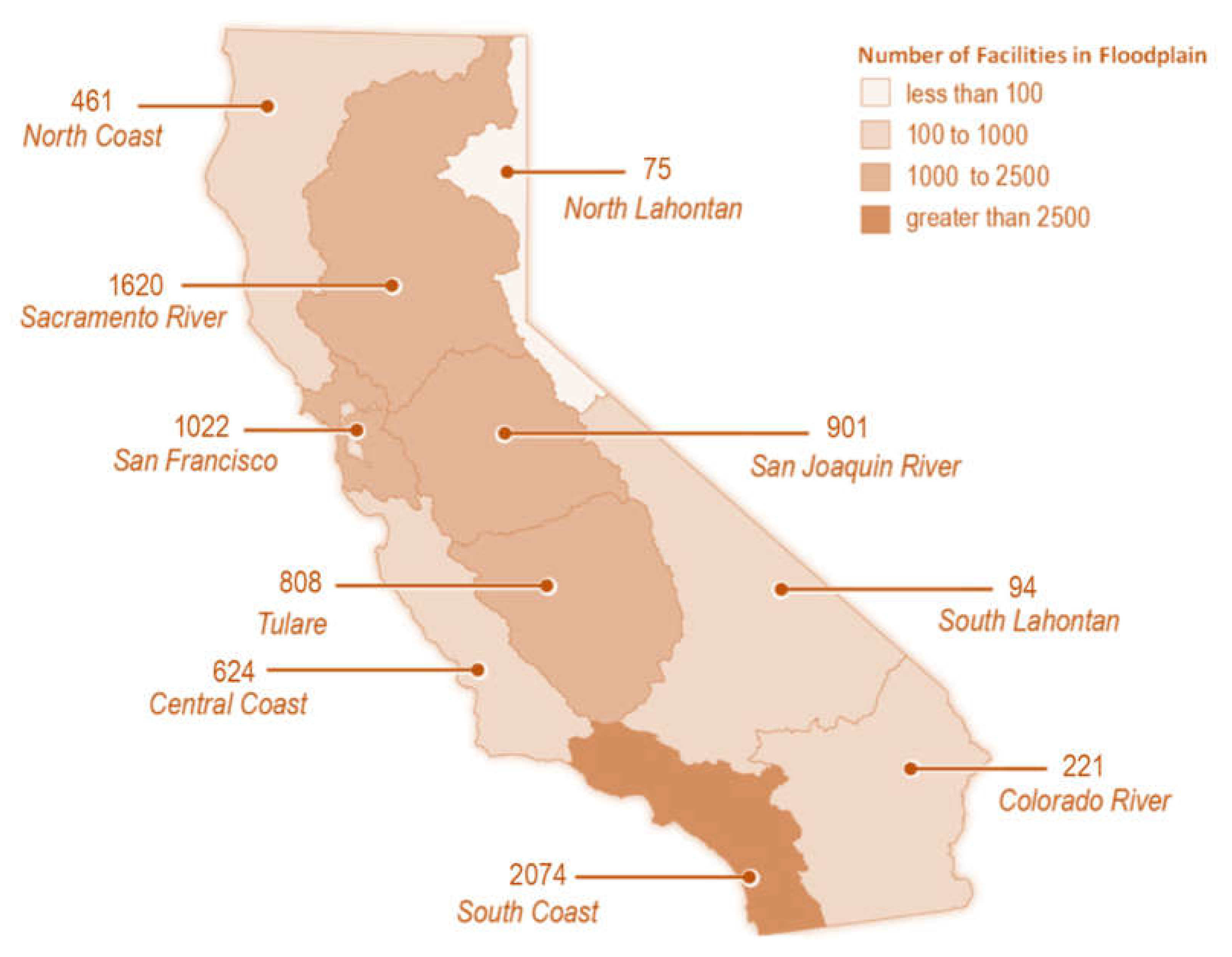
Southern California is particularly at risk for catastrophic flooding from multiple pathways, including flash flooding, stormwater flooding, debris flow flooding, tsunamis, and coastal storms. Coastal storms alone can put 873 miles of California roads at risk [26]. In addition, around 20% of California’s population lives on a floodplain, making decisions regarding California’s flood risk assessment vital to public safety. Despite the continuous investments in California’s transportation network expansion, the safety of this network is critically vulnerable to flooding. Of particular note is the South Coast hydrologic region (Figure 1), which has been found to contain over 2000 transportation facilities located within floodplains [27].
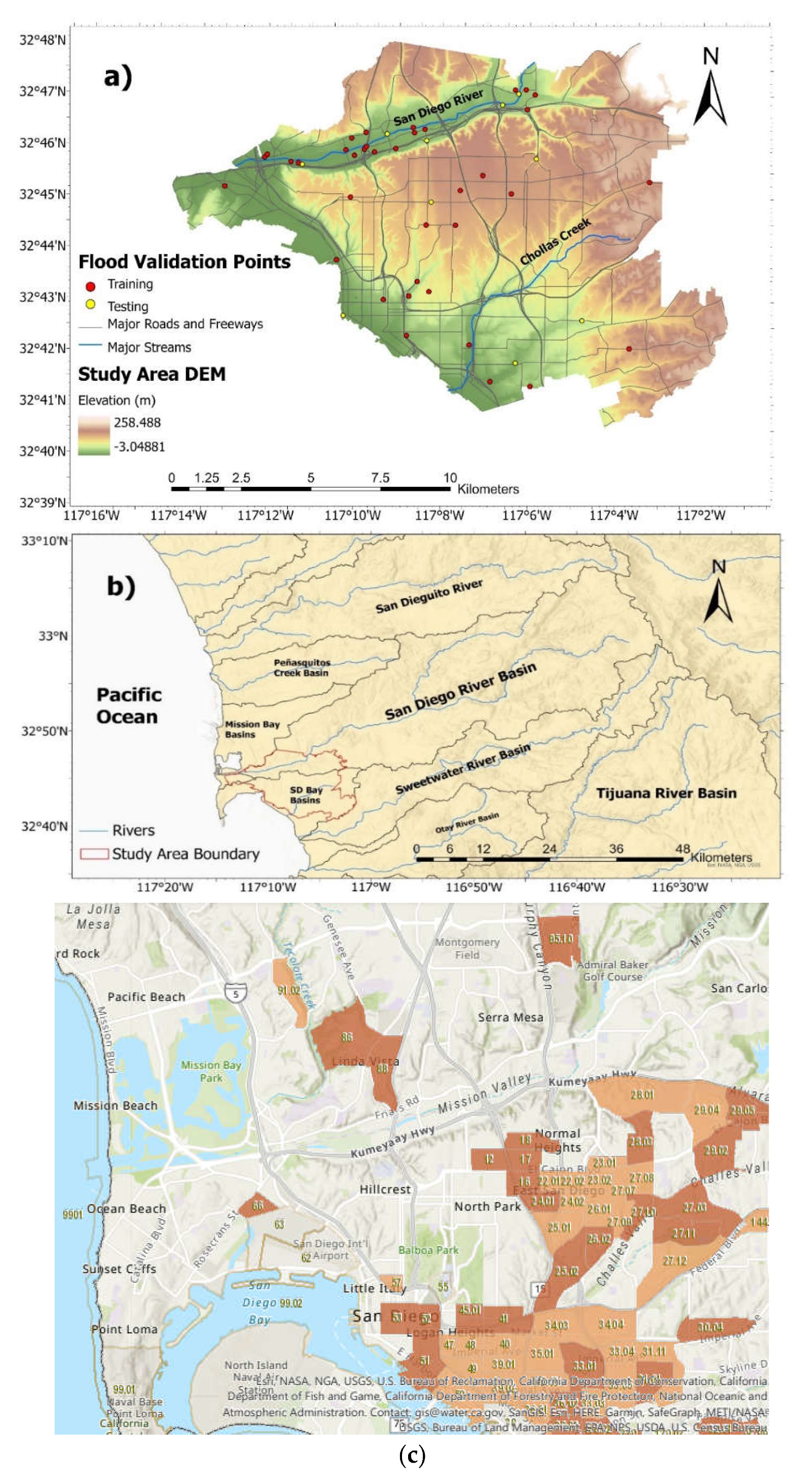
Figure 1 provides broader geographic and infrastructure context for the study area within the San Diego region, and this is shown in detail in Figure 2. The study area was chosen based on the following parameters: an area entirely within the extent of satellite images taken during times of flooding, an area with the necessary hydrologic data to create a flood risk model, and an area containing enough validation points for statistical significance. The San Diego Bay Basin meets these criteria. The region is entirely within the city of San Diego, covering about 155 mi2, and includes the flood-vulnerable Mission Valley area as well as disadvantaged neighborhoods such as City Heights and Barrio Logan, as shown in Figure 2C. The study area is the same for both the flood risk mapping and image classification portions of the study. The climate in the city is semi-arid Mediterranean, with long dry seasons and short wet seasons during the winter months. The climate, measured near the downtown in the south-western corner of the study area, is generally warm and mild, with maximum average monthly temperatures around 25 °C in August and September and average monthly lows in December and January of 14 °C. Precipitation is highly seasonal on both the coast and in the more humid highlands. The average precipitation in the city itself is 9.79 inches a year, with approximately three-quarters of this value falling between December and March.
In addition to carefully selecting the study area, storm events were also required to meet a specific criterion. The selection criteria for a storm we could study were one that occurred recently enough to be imaged by satellites equipped with high-resolution SAR, and one large enough to create enough flooding to be noted by news and police agencies. The selection of the area of interest and weather events for analysis will help to realize our goal of applying detection methods found to be effective for larger-scale flooding to events of a greater magnitude than have been studied previously.
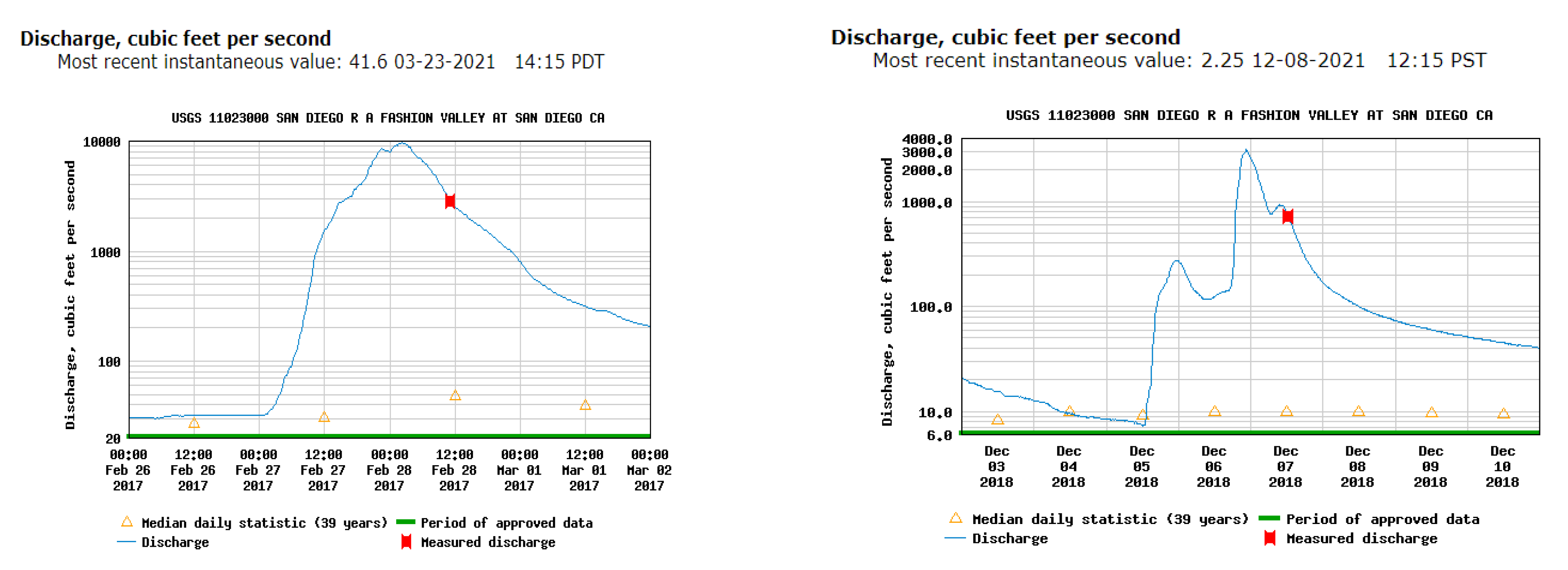
To assess the severity of a storm and the likely extent of flooding, we used rainfall and river stage data. While rainfall is far from homogenous across the San Diego area, we focused on the San Diego River at the Mission Valley community, as this is where most of the reported flooding occurred. Under the reasonable assumption that peak gauge height will correspond to peak flooding, we can use flood gauge data from the United States Geological Survey (USGS) to find peak storms over the past decade when high-resolution SAR sensors have been active. One gauge height peak immediately stands out, that for February of 2017. Closer inspection reveals that the gauge height reached a peak of almost 10,000 cfs at around 1:00 a.m. on 28 February 2017. Rainfall records also reflect a short, intense burst of rainfall that fell around 11:00 p.m. on the 27th—it was likely this high-intensity period of rainfall following steady rain the entire day beforehand that caused the high gauge height and flooding. Flooding for this day can be further verified with other qualitative data. A NOAA report, published in 2017, on heavy flooding through California in February of that year reported an “above-average” flood in Mission Valley on the 27th and 28th, reaching similar levels to historic peaks in 2011 and 1995 (2017). A Times of San Diego article reported enduring flooding on the 28th and evacuations in Lake Hodges and the Mission Valley area, as well as 702 collisions logged by the California Highway Patrol, nearly seven times the fair-weather average [28]. Roads reported as closed by police on the morning of 28 February 2017 were gathered with road closure data from another storm on 8 December 2018 as another source of data [29].
3. Methodology
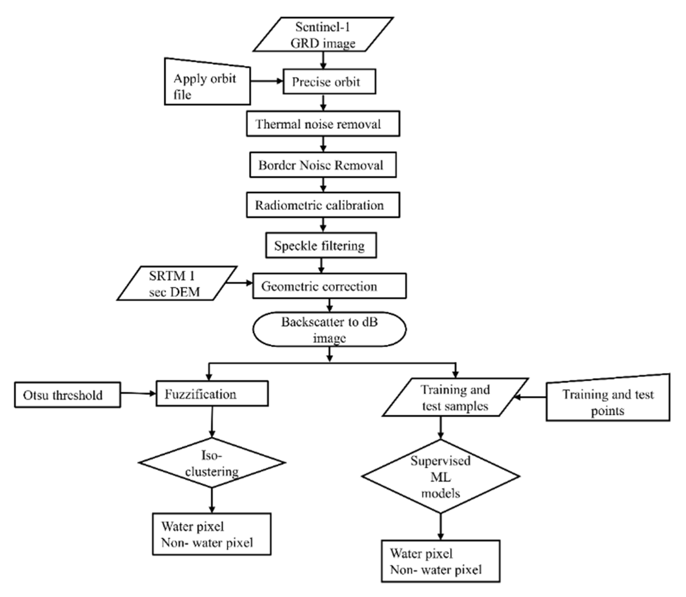
The stepwise image processing in the supervised and unsupervised machine learning method of this research is shown in Figure 3. Three supervised machine learning methods i.e., SVM, RF and MLC method are engaged. The reason for developing an unsupervised classification algorithm is (1) they are more robust than supervised classification algorithms in their application to early flood detection, and (2) no training datasets are required to set an unsupervised model. In addition to these, an unsupervised classification algorithm is also engaged to classify the flooded area. To obtain the supervised model datasets, first, image pre-processing has been done (Figure 3) using the European Space Agency Sentinel Application Platform (ESA SNAP) tool [30]. The purpose of image processing using the SNAP tool is to maintain consistent image properties of model datasets from multiple images. The workflow followed in the machine learning method is shown in Figure 3, including Sentinel 1 image processing from the raw dataset to backscatter intensity value generation, the unsupervised classification process, and the supervised classification process.
Sentinel-1’s revisit period is about six days, which means there is a significant possibility of missing flood images, and these should be taken during peak of floods. Based on the flood characteristics and timing described in the case study section, the obtained images (Table 1) from satellite were taken during two flood periods. This is verified by constructing flood hydrographs from streamflow measurements at the USGS gauge at the San Diego River Fashion Valley location [31] and checking the time these images are taken, which is within the flood periods. Multiple satellite images during both flood events are obtained, and those which better represent the time of flood peak, according to the USGS data, are selected (Figure 4).
3.1. Sentinel-1 Image Preprocessing Method
Sentinel 1 C band images (Table 1) are accessed from the Alaska archive. Sentinel 1, C band Interferometric Wide (IW) swath Ground Range Detected (GRD) datasets (Table 1) are chosen for mapping flooding in San Diego. The image preprocessing is done in a SNAP workflow that consists of seven major steps (1) application of the orbit file, (2) thermal noise removal, (3) border noise removal, (4) radiometric calibration, (5) speckle filtering, (6) geometric correction using Range doppler terrain correction, and (7) band conversion into decibels (dB). The first step of image preprocessing in SNAP is to correctly attribute the orbit state of SAR products [32]. When Sentinel level 1 products get updated in the archive, it takes several days-to-weeks to update the information about the orbit. Applying the correct information of the orbit file imposes the satellite position and velocity information in image acquisition. The next step of image preprocessing is thermal noise removal from the Sentinel-1 image. This image correction step removes any inter-sub-swath texture that may have been generated from two probable additive noise sources i.e., antenna patterns and scalloping noise [33]. The Border noise removal resamples the image with any curvature effect during acquisition, and it helps to remove the radiometric artefacts at the image borders caused by the time, azimuth, and range compression withal. The next step is radiometric calibration, which is a procedure of converting the digital numbers to radiometrically calibrated backscatter. It reverts an absolute calibration constant during level-1 product generation. The speckle noises appear in the SAR images as a granular noise that generates from the interaction of out of phase waves reflected from the earth scatterers. Lee speckle filter [34] at target window size 5 × 5 is applied for the proposed workflow. SAR images are subjected to some distortion by side looking geometry, which happens due to SAR images that are acquired with various viewing angles greater than 0 degrees, as well as with high-rise building structures. These distortions can be restored with orthorectification, which is a process known as terrain correction, e.g., range doppler terrain correction. This process converts the sensor coordinate to a map coordinate in a two-dimensional orthorectification process. The ESA SNAP toolbox is used to handle the Sentinel-1 GRD image preprocessing. The wet period images are obtained from Sentinel 1A GRD for the acquisition periods Feb 2017 and Dec 2018, while for dry period images it is obtained from Sentinel 1B. Sentinel-1A and Sentinel-1B capture images in ascending and descending orbit, respectively, and but they share the same orbit plane, with a 180° orbital phasing difference. Both Sentinel 1A and 1B GRD images have identical spectral properties. When both satellites are operational, Sentinel-1 requires a repeating cycle of about six days to complete a whole cycle for the earth’s observation.
3.2. Flood Mapping with Sentinel-1
A list of supervised and unsupervised machine learning methods which have been applied in this study is shown in Table 2. The supervised machine learning method considers SVM, RF, and MLC. The unsupervised classification algorithm that is developed in this study consists of Otsu thresholding, fuzzification and iso-clustering.
3.3. Model Datasets for Supervised Classification
The training dataset for the supervised classification model consists of 1000 random samples, including 800 ‘non-water’ and 200 ‘water’ pixels. Pixel information is extracted from the Sentinel-1 VH post-processed backscattering intensity dataset. Pixel information must be taken from a consistent satellite band, here the sentine-1 VH band, to eliminate the effect of temporal difference between dry and wet periods in images. The following steps are taken to extract modeling datasets:
- A total of three sentinel-1 images are obtained to extract the modeling datasets. Two images are taken during the wet period, during February 2017 and December 2018, and one image is obtained from a dry period, in March 2017 (Table 1), to be used for training supervised classification models. The description of modeling datasets is shown in Table 3.
- The Sentinel-1 VH image contains the backscattering intensity information. The SAR images have the advantage of not being covered by clouds in comparison to RGB pixel information in optical satellite images. The purpose of the supervised machine learning model is to classify the sentinel-1 VH band images during the flood event, i.e., classify pixels of images into water (such as waterbodies and flooded streets) and non-water pixels (vegetation, forest, developed area, open spaces and pavement, etc.) (Table 3).
- The input features of the supervised machine learning approach are the backscattering intensity which is extracted from the selected samples. The target variable is the label of a pixel, which can take one of the classes described in Table 3 depending on its backscattering intensity.
- About 800-pixel values from the ‘non-water’ pixel group are extracted to represent the dry period of the ‘March 2017′ image (Table 1). The pixel information is assigned as open space, vegetation, forest, developed area, or pavement type.
- The 200 water pixels consist of waterbodies and flooded street labels (Table 3). The post processed images during the San Diego floods of February 2017 and December 2018 were used to detect flood pixels. The ground truth data sourced from San Diego police road closure reports is used to assign and detect the flood pixels in the wet period images. The information regarding flood pixels were collected for 25 street locations. Since a total of 175 water pixels are represented by waterbodies, about 14 out of the remaining 25 pixels are used for training purposes and 11 pixels are kept for model validation.
- For the rest of the pixel types in the datasets, pixels are split into training and testing at the ratio of 80% and 20%, respectively (Table 3). The testing datasets are used later to verify the models’ prediction performance using accuracy assessment metrics.
3.4. Supervised Classification Method
3.4.1. Random Forest (RF)
In machine learning applications, Random Forest (RF) is an ensemble classification technique that utilizes the decision trees as one single tree in the forest. To create a set of controlled variance decision trees, the RF approach combines bootstrap aggregation (bagging) with random feature sorting. The RF has two parameters, i.e., the number of parameters and the depth of the decision trees that improve the classification accuracy. The depth of decision trees is determined by the number of features used to slice the nodes. The node impurity or the quality of a tree split is evaluated by ‘Gini’ (G), which was defined below in Equation (1) [35]:
Here, pi denotes the probability of a pixel classified in water pixel or non-water pixel class. The parameter optimization is done using the ‘GridSearchCV’ method available in scikit learn [36]. According to the hyperparameter tuning results, the maximum depth of trees found is 10, the minimum number of samples required to beat a leaf node is 3, the minimum number of samples required to split an internal node is 8, and the number of trees were set as 100.
3.4.2. Support Vector Machine
Support Vector Machine (SVM) is a widely used method in machine learning. The SVM method is a supervised classification technique that engages a hyperplane in a data space that divides the sentinel 1 pixel value in water and non-water objects. The SVM method offers several kernel functions including radial basis functions, linear, nonlinear, and polynomial functions. The flood image is classified by choosing the radial basis function, which can be expressed mathematically as Equation (1) [37]:
where the parameter controls the spread of the kernel. By tuning the parameter , the accuracy of the water and non-water pixels is increased. The hyperparameter tuning is done using the ‘GridSearchCV’ method in the sci-kit learn package of python. The model set up is obtained optimally with the radial basis function as a kernel function, with the regularization parameter equal to 10.
3.4.3. Maximum Likelihood Classification
The ArcGIS maximum likelihood classification (MLC) tool is used to classify the Sentinel 1 post processed images. The tool works based on the assumption that the samples assigned under each class are normally distributed. When attributing each cell to one of the classes contained in the signature file, the tool considers both the variances and covariances of the class signatures. The mean vector and the covariance matrix can be applied to identify a class under the assumption that the class sample is normally distributed. The statistical probability for each class is computed using these two features for each cell value to evaluate the cells’ membership in a class. The prior probability weight of each class is set as ‘equal’ for running the MLC tool in ArcGIS (ESRI, Redlands, CA, USA).
3.4.4. Change Detection using Unsupervised Classification Method
The unsupervised classification method engaged in this study utilized the post processed Sentinel 1 image in three steps: (1) determining the Otsu threshold [23], fuzzification, and iso-clustering. Assume that each pixel in an image is represented by L gray levels (1,2, …, L). Let N denote the total number of pixels, and ni signify the number of pixels at level i. The likelihood that level i will occur is given by pi = ni/N. Let us allow a threshold T to divide a sentinel 1 image pixel into two classes C0 and C1. C0 is made up of pixels with the levels [1, ⋯, T] and C1 made up of pixels with the levels [T + 1, ⋯, L]. Let P0(T) and P1(T) denote the cumulative probabilities, μ0(T) denote the mean levels, and μ1(T) denote the variances of the classes C0 and C1, respectively. These values are given by:
Let μ, , and denote the image’s mean level, between-class variance, and within-class variance, respectively.
According to Otsu, the threshold determined via maximization of between-class variance is:
This value is the same as the threshold determined by minimizing within-class variances:
Furthermore, the above threshold is identical to the ones determined by maximizing the ratio of between-class to within-class variations [38]. The threshold obtained following Otsu was later used to apply the fuzzy large function. This threshold selection process maximizes the variance among the water and non-water pixels. This function is used to enhance the class distance between water and non-water pixels, making it easier to distinguish between the two classes in iso-clustering. When the larger input values are more likely to be a member of the set, the fuzzy large transformation function is applied. The following is the definition of the fuzzy large function:
where x is the raster value of a sentinel 1 image, f1 and T are respectively spread and Otsu threshold in raster value distribution. After fuzzification the iso-clustering is done using the Iso Cluster Unsupervised Classification tool in ArcGIS. The Iso Cluster uses an improved iterative optimization procedure of clustering and then fit a maximum likelihood function to transform the pixel cluster in a normally distributed cluster. Thus, the iso-cluster tool extracts the samples that has the unimodal distribution in the sentinel 1 data. Since after fuzzification the class variance between the water and non-water classes are more pronounced, the maximum likelihood function to get two distinct classes is easy to fit by using the iso clustering tool. The functionality of the iso-clustering tool for unsupervised classification is more detailed in ArcGIS (2021).
In order to find the change in water extent during dry and wet periods at first the unsupervised classification is done over the wet image, then the model is re-run over the image acquired during the dry period (March 2017). Based on the difference between the dry and wet period, the change is detected as the inundation extent.
3.4.5. Accuracy Assessment Metrics
Four machine learning method accuracy metrics i.e., (a) Precision (Equation (13)), (b) Recall (Equation (14)), (c) F1-score (Equation (15)), (d) Accuracy (Equation (16)) are engaged to measure the classification accuracy from the supervised and unsupervised classification in this study [39]. The ranges of these metrics vary between 0 to 1, and the greater the value of these metrics, the better the model performance. These metrics are required to calculate the true positive (TP), true negative (TN), false positive (FP), and false negative (FN) samples in the testing datasets. The true positive (TP) samples are those pixels in which the machine learning model correctly detects the true classified pixel type as the water pixel in the prediction. The true negative (TN) pixels are non-water pixels in observation correctly detected as non-water pixels in the machine learning prediction. The false positive (FP) samples are incorrectly detected as water pixels, which are non-water pixels in observed datasets. The false negative (FN) samples are the non-water pixels detected by the machine learning model, which are water pixels in the observed datasets.
where, TP, FP, TN, and FN are respectively true positive (TP), true negative (TN), false positive (FP), and false negative (FN) samples.
4. Results and Discussions
4.1. Accuracy Assessment
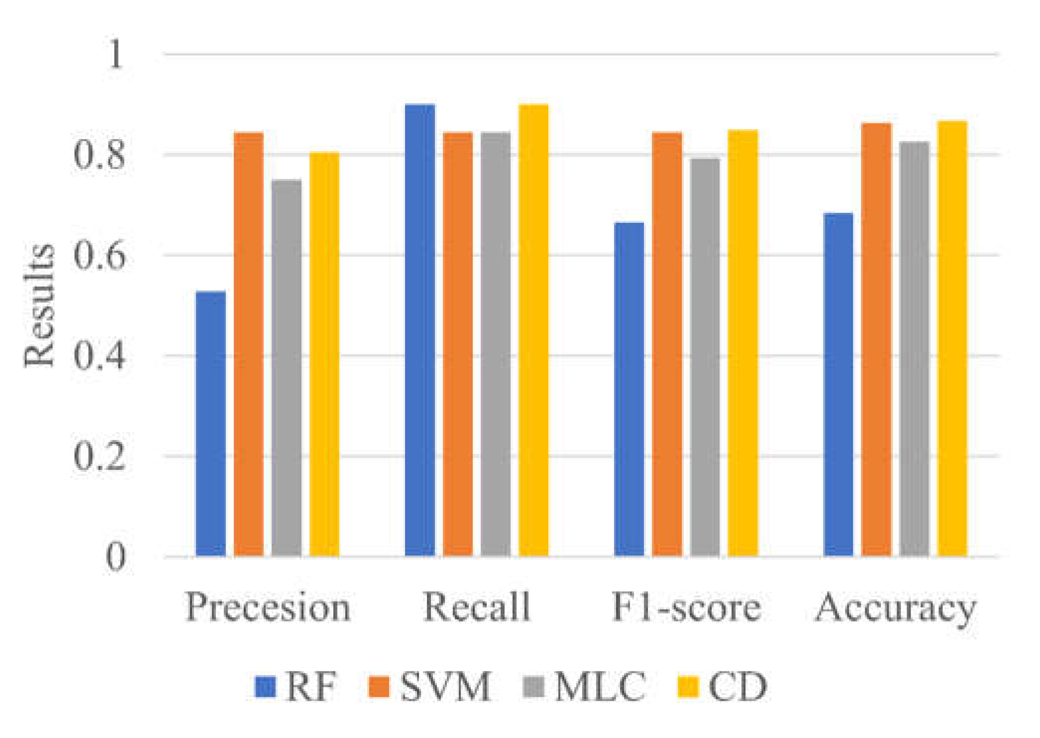
The performance of machine learning models in classifying water and non-water pixels are shown in Figure 5. Using the testing datasets of RF, SVM, MLC and CD shows a precision of 0.53, 0.85, 0.75 and 0.81 respectively, the recall values of 0.9, 0.85, 0.85 and 0.9 respectively, the F1-score is obtained as 0.67, 0.85, 0.79 and 0.85, respectively, and the accuracy is 0.69, 0.87, 0.83 and 0.87, respectively. Considering the performance metrics, the SVM and CD method achieved the highest accuracy among the four methods. Overall, our observations show that the flood pixels in Sentinel 1 images were mixed up with the pavements pixels in many places. This is the reason for the misclassification overestimation in the flood extent in many locations.
4.2. Flood Mapping with Supervised Classification
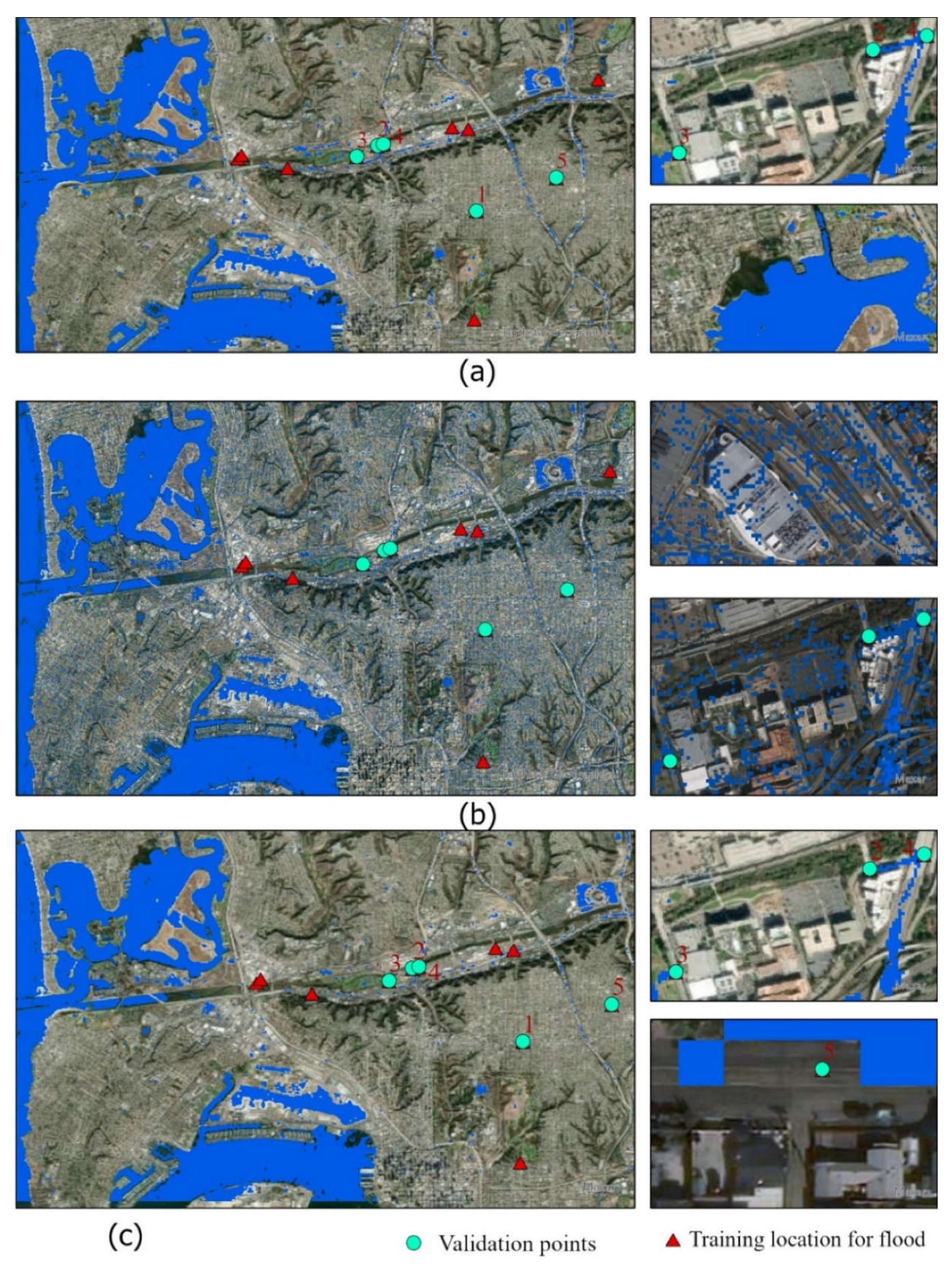
Figure 6 visually displays the results of the MLC, RF, and SVM flood image processing techniques. Flood maps created using the MLC (Figure 6a) and SVM (Figure 6c) techniques boast accuracy scores above 0.8, and the maps derived from those techniques are similar. Flood patterns are easily visible and vulnerable areas where flooding is predicted are shown in blue. The map derived using the RF technique (Figure 6b) produced a much less precise map with a significantly lower accuracy score. A closer look at the map reveals extremely scattered flood pixels that do not conform to the same patterns that emerged using the other more accurate and precise techniques. In addition, artifacts of flooding from the RF are impossibly located. As shown in the detailed images to the right of the RF map, flooded pixels occur in areas such as rooftops that are not affected by flooding. Performance metrics shown in the bar graph of Figure 5 reflect these observations and provide insight into the varied accuracy of each supervised method.
4.3. Flood Mapping with Unsupervised Classification
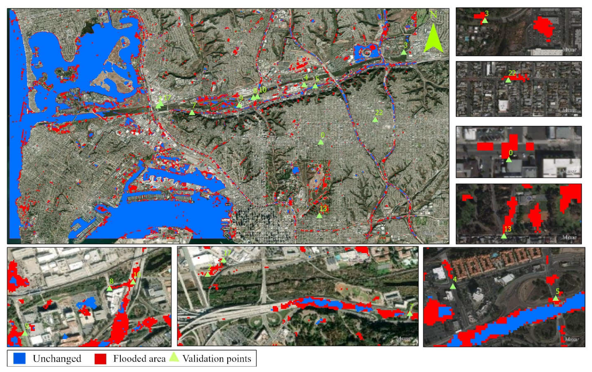
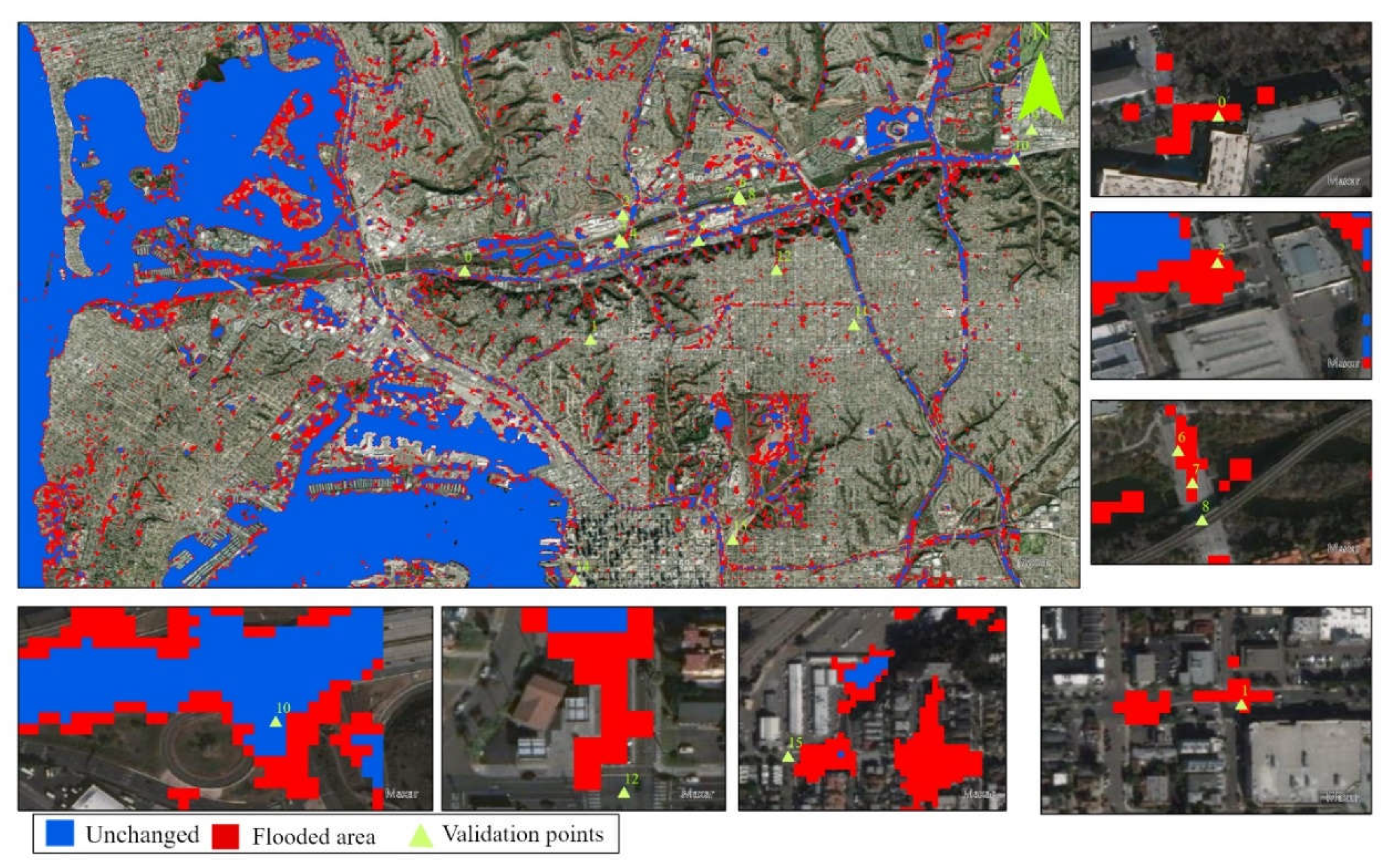
The results of the Change Detection method used to define the extent of inundation are shown in Figure 7 and Figure 8. The unchanged pixels in Figure 8 are retained in same ‘non-water’ pixels comparing both wet and dry period images. Despite the potential for inaccurate results, the unsupervised techniques can produce the same as the most successful supervised technique. This achievement is represented visually for the 2017 flood scenario and the 2018 flood scenario in Figure 7 and Figure 8, respectively. Results are also represented graphically in Figure 5. High rates of overlap between unchanged zones and flooded areas that can be seen in the maps of Figure 7 and Figure 8 reflect the high levels of accuracy shown in Figure 5 for the change detection method. The patterns of flooding created using change detection showcase the high levels of precision attained using the unsupervised method. Unsupervised classification generally takes more computing power while requiring less human input. This is a valuable consideration in assessing performance metrics and discussing the results of each technique being implemented to recreate flood maps.
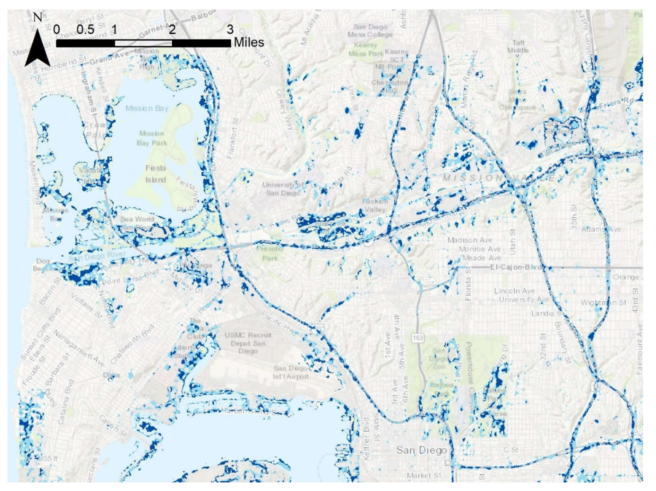
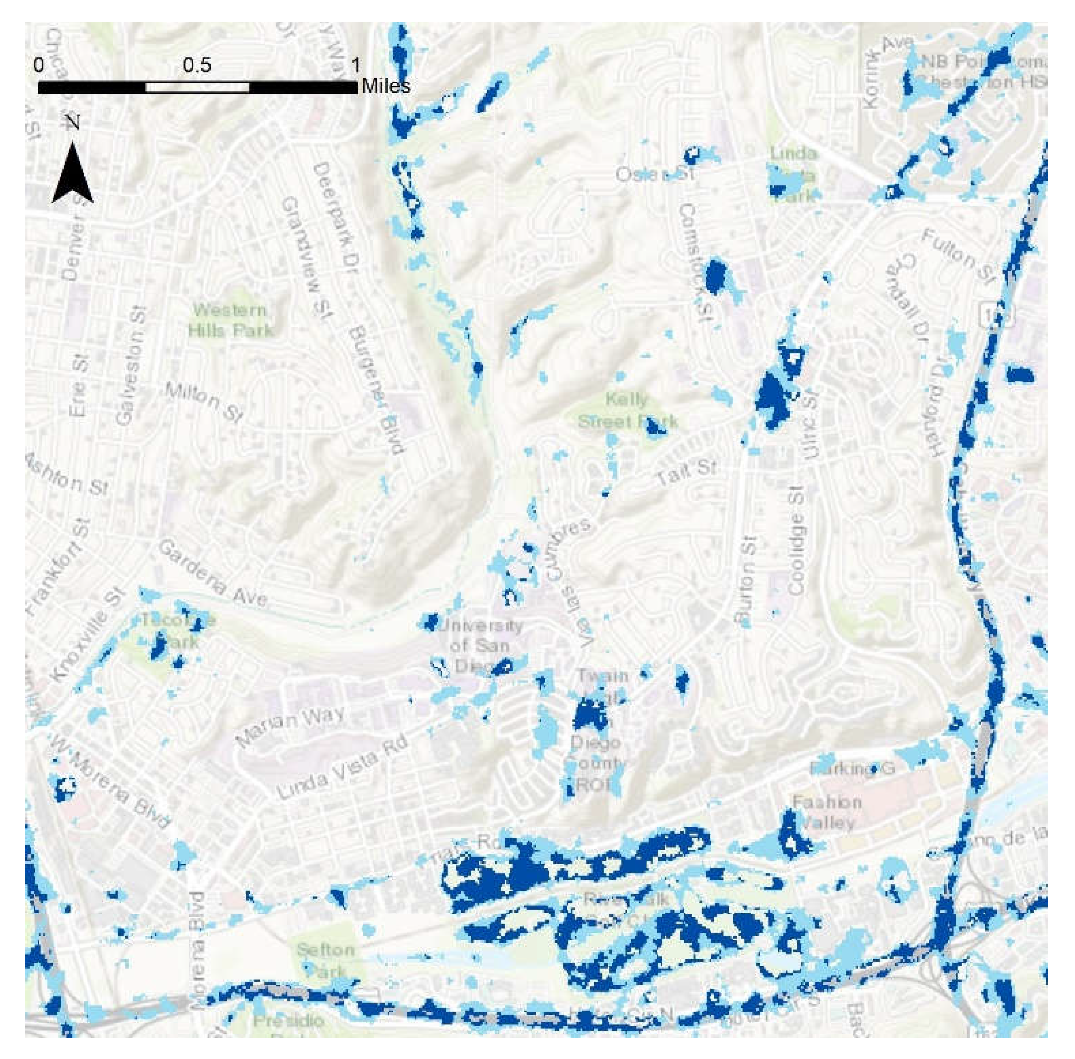
In order to identify the frequently flooded areas in our study region, Figure 9, Figure 10, Figure 11, Figure 12, Figure 13 and Figure 14 are presented based on the model with the best performance, i.e., Change Detection. Figure 9 depicts the entirety of the flood data collected throughout a coastal section of Southern San Diego County during rain events that occurred on 28 February 2017, and on 8 December 2018. Light blue shading represents areas that experienced flooding in either the 2017 or 2018 weather events, while dark blue shadings represent areas flooded by both the 2017 and 2018 weather events. As shown by the map, many instances of flooding are in close proximity to existing bodies of water such as the Pacific Ocean, the San Diego Bay, Mission Bay, and the San Diego River. Other significant flood patterns include the high coverage of San Diego’s major roads and freeways. The blue shading along the lines of Interstates 8, 805, 15 and other roadways indicates potentially hazardous road conditions or possible roadway closures. Subareas of particular interest include Mission Valley, Point Loma, Downtown, Mission Bay, and Fashion Valley. These areas highlight the use of flood detection for reducing risk through each of their unique facilities that can be affected by flooding events.
The Mission Valley area shown in Figure 10 is especially vulnerable to flooding events that affect road conditions, commercial buildings, and shopping centers. The Westfield Mission Valley mall is often affected during heavy rainfall events and can create hazardous conditions for patrons. Road closures and restricted building access can also be attributed to flood events of this magnitude. Increased flood detection can minimize the exposure of pedestrians and drivers to hazardous conditions by improving city responses and flood management efforts in areas where flooding is detected.
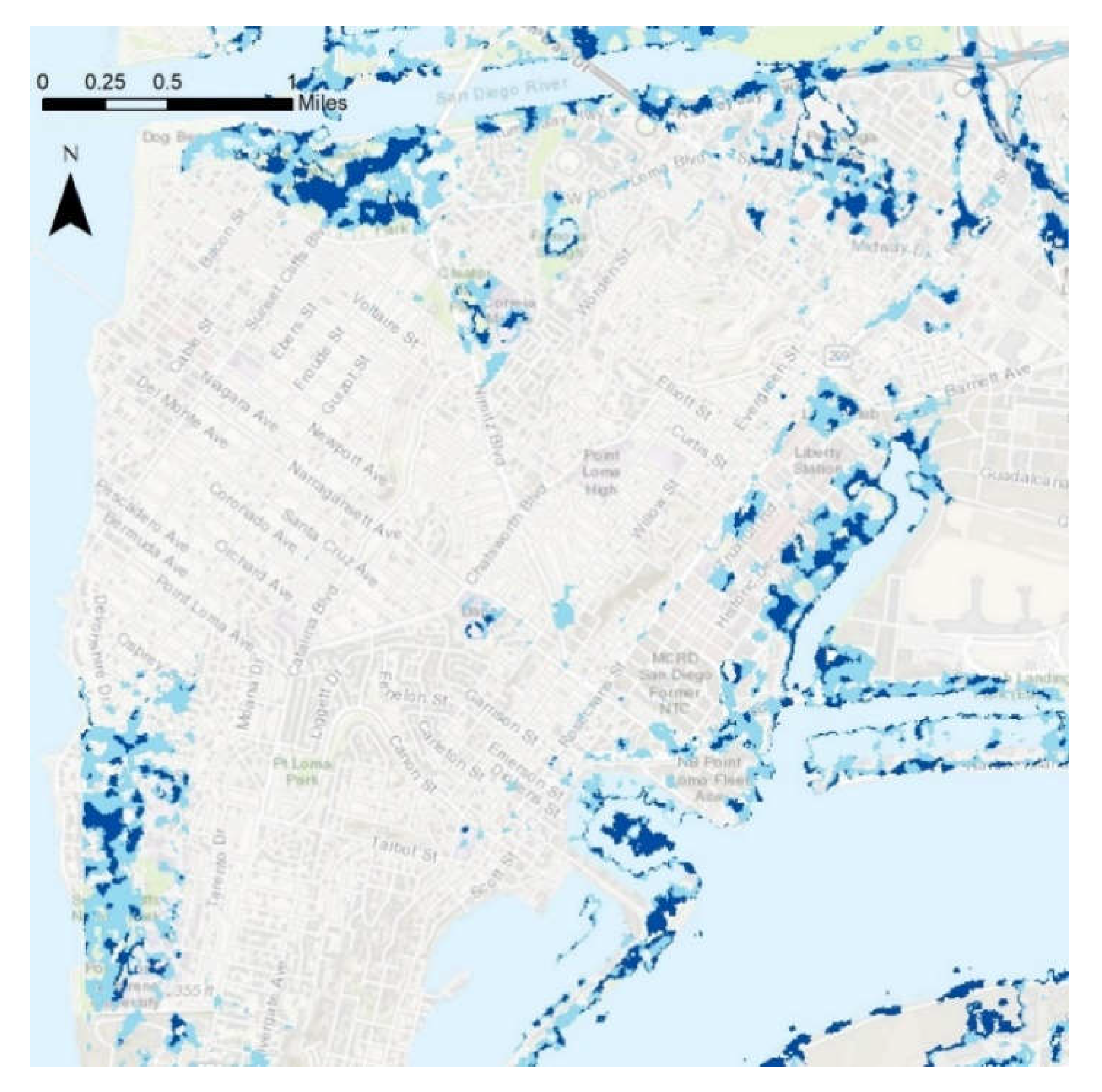
Point Loma (Figure 11) is a waterfront community bordered by the San Diego River to the North, the San Diego Bay to the South, and the Pacific Ocean to the West. This area is home to many highly trafficked landmarks including Liberty Station, Pechanga Arena, and Sunset Cliffs Natural Park. This snapshot makes it apparent that flooding occurs at a greater extent near existing bodies of water and because the area is surrounded by water on three sides, it is exceptionally vulnerable to flooding events The geography of the affected areas includes low-lying land and shallow groundwater. These factors are likely responsible for increased incidences of flooding during rain events. These floods have the potential to create hazardous road conditions and may even require road closures in heavily affected areas. Increased levels of flood detection in this area would help bolster risk management in relation to flooding events where drivers and community members may find themselves at risk of bodily harm or property damage.
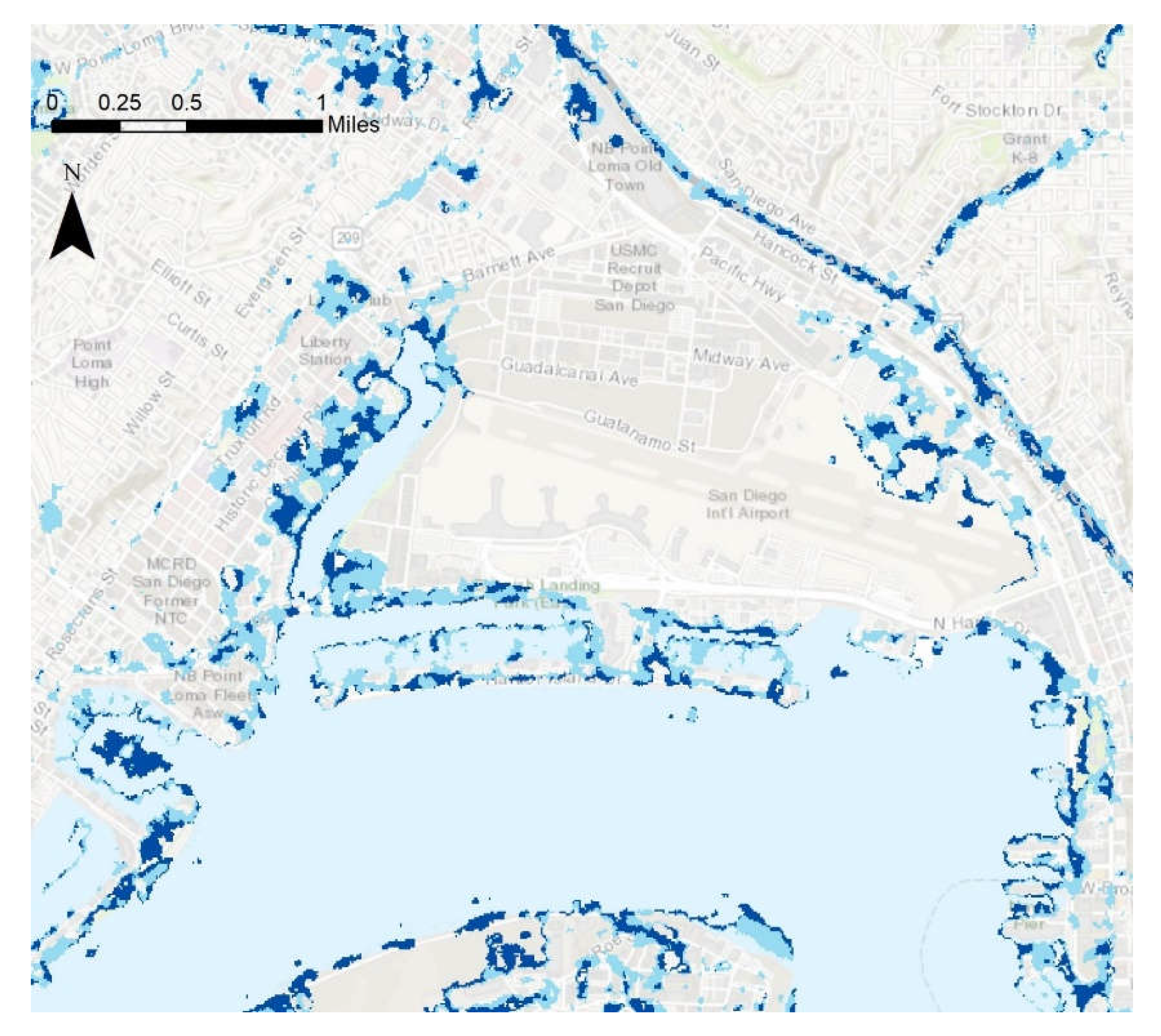
Instances of flooding that occurred at the San Diego International Airport (Figure 12) are represented by the shading in the map above. The airport is extremely vital to the city and is located directly on the San Diego Bay in Downtown San Diego. Flooding instances occurred in both 2017 and 2018. As the climate continues to change, sea level rise and increased frequencies of extreme weather events continue to raise the flood risk to the airport. Unsafe runway conditions, flood damage, and variable levels of accessibility are potentially hazardous to patrons and employees at the airport. Unsafe road conditions entering and exiting the airport due to flooding are hazardous because of the heavily trafficked nature of the roads that lead to and from the airport. The ability to accurately detect and map flooding patterns at this location would improve the safety of the airport and could allow for more long-term solutions to be implemented to improve the facility’s resilience, as flood risk in the area will only increase in the future with climate change and rising sea levels.
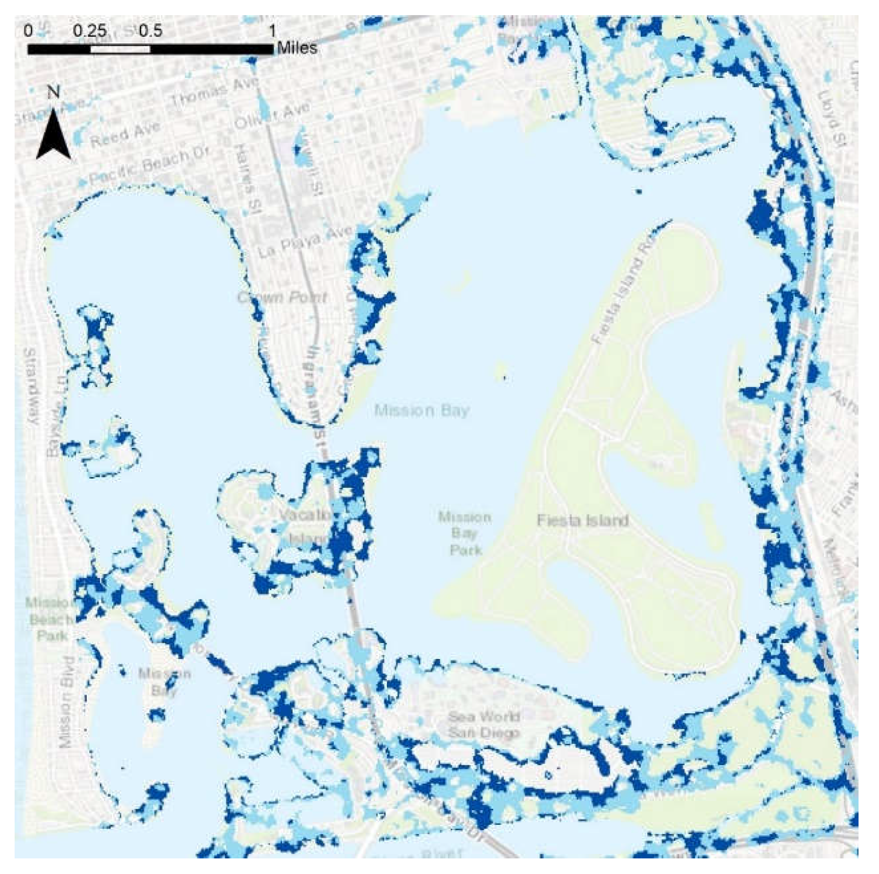
The low-lying area of Mission Bay (Figure 13) is susceptible to flooding, as shown in the patterns depicted above. Flood detection will help to distinguish usable facilities in an efficient manner and will help improve safety factors in the area featuring boat launches, beaches, parks, and bike paths. Flooding begins at the interface between the land and water and creeps towards important recreational areas, including the extensive Mission Bay Park and Sea World. As shown by flooding on streets that occurred during both the 2017 and 2018 rain events, access to the area may become hindered and roadway safety is a concern.
Fashion Valley (Figure 14) is bordered by the San Diego River and is home to the commercially important Fashion Valley Mall. The area is prone to flooding and is often inundated by urban flooding following rain events, as is shown by the extent that occurred in both 2017 and 2018. Flooding events disrupt daily business practices and reduce parking capacity. The overall safety of the busy mall following weather events will be improved by implementing more efficient flood detections such as the techniques exemplified in this text.
5. Conclusions
The paper presents a comprehensive comparison of different machine learning methods for image processing of satellite scenes under wet and dry conditions. Our approach presents an unsupervised flood image classification, i.e., CD can provide a more robust solution for flood mapping. This systematic approach can be useful in urban flood mapping, particularly with regard to handling the flood risk in transportation facilities.
Author Contributions
A.H.T. Formal Analysis, Software, Writing-Original Draft, C.B.M. Writing-Review and Editing, Visualization, H.T.-D. Project Administration, Funding Acquisition, Supervision, E.G. Data Curation, Writing-Review and Editing. All authors have read and agreed to the published version of the manuscript.
Funding
This research was funded by the Office of the Assistant Secretary for Research and Technology, University Transportation Centers Program, Department of Transportation (Safe-D National UTC), Grant Number: 69A3551747115.
Institutional Review Board Statement
Not applicable.
Informed Consent Statement
Not applicable.
Data Availability Statement
All the data used in the study will be available upon request.
Acknowledgments
This research has been supported by the Office of the Assistant Secretary for Research and Technology, University Transportation Centers Program, Department of Transportation (Safe-D National UTC), Grant Number: 69A3551747115, Project Number: 05-101.
Conflicts of Interest
The authors declare no conflict of interest.
References
- Henonin, J.; Russo, B.; Mark, O.; Gourbesville, P. Real-time urban flood forecasting and modelling–a state of the art. J. Hydroinformatics 2013, 15, 717–736. [Google Scholar] [CrossRef]
- De Almeida, G.; Bates, P.; Ozdemir, H. Modelling urban floods at submetre resolution: Challenges or opportunities for flood risk management? J. Flood Risk Manag. 2018, 11, S855–S865. [Google Scholar] [CrossRef] [Green Version]
- Moftakhari, H.R.; AghaKouchak, A.; Sanders, B.F.; Allaire, M.; Matthew, R.A. What Is Nuisance Flooding? Defining and Monitoring an Emerging Challenge. Water Resour. Res. 2018, 54, 4218–4227. [Google Scholar] [CrossRef]
- Moftakhari, H.R.; AghaKouchak, A.; Sanders, B.F.; Feldman, D.L.; Sweet, W.; Matthew, R.A.; Luke, A. Increased nuisance flooding along the coasts of the United States due to sea level rise: Past and future. Geophys. Res. Lett. 2015, 42, 9846–9852. [Google Scholar] [CrossRef] [Green Version]
- Alsdorf, D.E.; Rodríguez, E.; Lettenmaier, D.P. Measuring surface water from space. Rev. Geophys. 2007, 45, 1–24. [Google Scholar] [CrossRef]
- Tong, X.; Luo, X.; Liu, S.; Xie, H.; Chao, W.; Makhinova, A.; Jiang, Y. An approach for flood monitoring by the combined use of Landsat 8 optical imagery and COSMO-SkyMed radar imagery. ISPRS J. Photogramm. Remote Sens. 2018, 136, 144–153. [Google Scholar] [CrossRef]
- Tanguy, M.; Chokmani, K.; Bernier, M.; Poulin, J.; Raymond, S. River flood mapping in urban areas combining Radarsat-2 data and flood return period data. Remote Sens. Environ. 2017, 198, 442–459. [Google Scholar] [CrossRef] [Green Version]
- Giustarini, L.; Hostache, R.; Matgen, P.; Schumann, G.J.-P.; Bates, P.D.; Mason, D.C. A change detection approach to flood mapping in urban areas using TerraSAR-X. IEEE Trans. Geosci. Remote Sens. 2012, 51, 2417–2430. [Google Scholar] [CrossRef] [Green Version]
- Matgen, P.; Hostache, R.; Schumann, G.; Pfister, L.; Hoffmann, L.; Savenije, H. Towards an automated SAR-based flood monitoring system: Lessons learned from two case studies. Phys. Chem. Earth Parts A/B/C 2011, 36, 241–252. [Google Scholar] [CrossRef]
- Mason, D.C.; Speck, R.; Devereux, B.; Schumann, G.J.-P.; Neal, J.C.; Bates, P.D. Flood detection in urban areas using TerraSAR-X. IEEE Trans. Geosci. Remote Sens. 2009, 48, 882–894. [Google Scholar] [CrossRef] [Green Version]
- Mason, D.; Giustarini, L.; Garcia-Pintado, J.; Cloke, H. Detection of flooded urban areas in high resolution Synthetic Aperture Radar images using double scattering. Int. J. Appl. Earth Obs. Geoinf. 2014, 28, 150–159. [Google Scholar] [CrossRef] [Green Version]
- Pulvirenti, L.; Chini, M.; Pierdicca, N.; Boni, G. Use of SAR Data for Detecting Floodwater in Urban and Agricultural Areas: The Role of the Interferometric Coherence. IEEE Trans. Geosci. Remote Sens. 2015, 54, 1532–1544. [Google Scholar] [CrossRef]
- Li, Y.; Martinis, S.; Plank, S.; Ludwig, R. An automatic change detection approach for rapid flood mapping in Sentinel-1 SAR data. Int. J. Appl. Earth Obs. Geoinf. 2018, 73, 123–135. [Google Scholar] [CrossRef]
- Shahabi, H.; Shirzadi, A.; Ghaderi, K.; Omidvar, E.; Al-Ansari, N.; Clague, J.J.; Geertsema, M.; Khosravi, K.; Amini, A.; Bahrami, S.; et al. Flood Detection and Susceptibility Mapping Using Sentinel-1 Remote Sensing Data and a Machine Learning Approach: Hybrid Intelligence of Bagging Ensemble Based on K-Nearest Neighbor Classifier. Remote Sens. 2020, 12, 266. [Google Scholar] [CrossRef] [Green Version]
- Tavus, B.; Kocaman, S.; Gokceoglu, C. Flood damage assessment with Sentinel-1 and Sentinel-2 data after Sardoba dam break with GLCM features and Random Forest method. Sci. Total Environ. 2021, 816, 151585. [Google Scholar] [CrossRef]
- Gašparović, M.; Dobrinić, D. Comparative Assessment of Machine Learning Methods for Urban Vegetation Mapping Using Multitemporal Sentinel-1 Imagery. Remote Sens. 2020, 12, 1952. [Google Scholar] [CrossRef]
- Chen, H.; Chandrasekar, V.; Cifelli, R.; Xie, P. A Machine Learning System for Precipitation Estimation Using Satellite and Ground Radar Network Observations. IEEE Trans. Geosci. Remote Sens. 2019, 58, 982–994. [Google Scholar] [CrossRef]
- Radhakrishnan, C.; Chandrasekar, V.; Berg, W.; Reising, S.C. Rainfall Estimation from Tempest-D Cubesat Observations. In Proceedings of the 2021 IEEE International Geoscience and Remote Sensing Symposium IGARSS, Brussels, Belgium, 14 July 2021; pp. 8115–8118. [Google Scholar]
- Hosseiny, H.; Nazari, F.; Smith, V.; Nataraj, C. A Framework for Modeling Flood Depth Using a Hybrid of Hydraulics and Machine Learning. Sci. Rep. 2020, 10, 8222. [Google Scholar] [CrossRef]
- Schubert, J.E.; Sanders, B.F. Building treatments for urban flood inundation models and implications for predictive skill and modeling efficiency. Adv. Water Resour. 2012, 41, 49–64. [Google Scholar] [CrossRef]
- Cao, H.; Zhang, H.; Wang, C.; Zhang, B. Operational Flood Detection Using Sentinel-1 SAR Data over Large Areas. Water 2019, 11, 786. [Google Scholar] [CrossRef] [Green Version]
- Chawla, I.; Karthikeyan, L.; Mishra, A.K. A review of remote sensing applications for water security: Quantity, quality, and extremes. J. Hydrol. 2020, 585, 124826. [Google Scholar] [CrossRef]
- Otsu, N. A threshold selection method from gray-level histograms. IEEE Trans. Syst. Man Cybern. 1979, 9, 62–66. [Google Scholar] [CrossRef] [Green Version]
- Vanama, V.S.K.; Rao, Y.S. Change detection based flood mapping of 2015 flood event of Chennai city using sentinel-1 SAR images. In Proceedings of the IGARSS 2019–2019 IEEE International Geoscience and Remote Sensing Symposium, Yokohama, Japan, 28 July–2 August 2019; IEEE: Piscataway, NJ, USA, 2019. [Google Scholar]
- Fernandez-Prieto, D.; Marconcini, M. A novel partially supervised approach to targeted change detection. IEEE Trans. Geosci. Remote Sens. 2011, 49, 5016–5038. [Google Scholar] [CrossRef]
- NOAA. Heavy Precipitation Events California and Northern Nevada January and February 2017. Available online: https://www.cnrfc.noaa.gov/storm_summaries/janfeb2017storms.php (accessed on 10 December 2021).
- Ehlers, R.; Brown, B. Managing Floods in California; Legislative Analyst’s Office: Sacremento, CA, USA, 2017; pp. 1–10. [Google Scholar]
- Jennewein, C. Record Rain Is Over, but Flooding Remains a Major Problem; Times of San Diego: San Diego, CA, USA, 2017. [Google Scholar]
- Robbins, G. Flash Flood Warning for San Diego Area Expires, but many Roadways Remain Inundated; The San Diego Union Tribune: San Diego, CA, USA, 2018. [Google Scholar]
- Zuhlke, M.; Fomferra, N.; Brockmann, C.; Peters, M.; Veci, L.; Malik, J.; Regner, P. SNAP (sentinel application platform) and the ESA sentinel 3 toolbox. Sentin.-3 Sci. Workshop 2015, 734, 21. [Google Scholar]
- USGS. USGS Streamflow Measuring Station. 11023000 San Diego R a Fashion Valley at San Diego, CA. Available online: https://waterdata.usgs.gov/ca/nwis/uv/?site_no=11023000&PARAmeter_cd=00065,00060 (accessed on 7 December 2021).
- Filipponi, F. Sentinel-1 GRD preprocessing workflow. In Multidisciplinary Digital Publishing Institute Proceedings; Italian National Institute for Environmental Protection and Research: Rome, Italy, 2019. [Google Scholar]
- Mascolo, L.; Lopez-Sanchez, J.M.; Cloude, S.R. Thermal Noise Removal From Polarimetric Sentinel-1 Data. IEEE Geosci. Remote Sens. Lett. 2021, 19, 4009105. [Google Scholar] [CrossRef]
- Lee, J.-S.; Wen, J.-H.; Ainsworth, T.L.; Chen, K.-S.; Chen, A.J. Improved sigma filter for speckle filtering of SAR imagery. IEEE Trans. Geosci. Remote Sens. 2008, 47, 202–213. [Google Scholar]
- Svetnik, V.; Liaw, A.; Tong, C.; Culberson, J.C.; Sheridan, R.P.; Feuston, B.P. Random Forest: A Classification and Regression Tool for Compound Classification and QSAR Modeling. J. Chem. Inf. Comput. Sci. 2003, 43, 1947–1958. [Google Scholar] [CrossRef]
- Pedregosa, F.; Varoquaux, G.; Gramfort, A.; Michel, V.; Thirion, B.; Grisel, O.; Blondel, M.; Prettenhofer, P.; Weiss RDubourg, V. Scikit-learn: Machine learning in Python. J. Mach. Learn. Res. 2011, 12, 2825–2830. [Google Scholar]
- Keerthi, S.S.; Shevade, S.K.; Bhattacharyya, C.; Murthy, K.R.K. Improvements to Platt’s SMO Algorithm for SVM Classifier Design. Neural Comput. 2001, 13, 637–649. [Google Scholar] [CrossRef]
- Sahoo, P.; Soltani, S.; Wong, A. A survey of thresholding techniques. Comput. Vision Graph. Image Process. 1988, 41, 233–260. [Google Scholar] [CrossRef]
- Han, J.; Pei, J.; Kamber, M. Data Mining: Concepts and Techniques; Elsevier: North York, ON, Canada, 2011. [Google Scholar]
Figure 1.
Transportation facilities within the floodplains by California hydrologic regions. Transportation facilities include highways, railroads, public transportation facilities, airports, etc. data from [27].
Figure 1.
Transportation facilities within the floodplains by California hydrologic regions. Transportation facilities include highways, railroads, public transportation facilities, airports, etc. data from [27].

Figure 2.
Figures of location and geographic context of study area. (a) shows study area DEM, network of major roads, major streams, and validation points. (b) shows hydrologic and geographic context of region around the study area. (c) Disadvantaged communities by census tract in the study area as designated by CalEnviroScreen.3 (light orange: Disadvantaged, dark orange: Severely Disadvantaged).

Figure 3.
Flowchart of the Sentinel 1 image processing in supervised and unsupervised machine learning method.
Figure 3.
Flowchart of the Sentinel 1 image processing in supervised and unsupervised machine learning method.

Figure 4.
Image acquisition time marked as red points on the flood hydrograph for wet scenes. Left: March 2017 event. Right: December 2018 event.
Figure 4.
Image acquisition time marked as red points on the flood hydrograph for wet scenes. Left: March 2017 event. Right: December 2018 event.

Figure 5.
The model performance metrics of four different machine learning models in terms of precision, recall, F1 score and Accuracy.
Figure 5.
The model performance metrics of four different machine learning models in terms of precision, recall, F1 score and Accuracy.

Figure 6.
2017 Flood image processing using (a) Maximum Likelihood Classifier, (b) Random Forest (c) Support Vector Machine.
Figure 6.
2017 Flood image processing using (a) Maximum Likelihood Classifier, (b) Random Forest (c) Support Vector Machine.

Figure 7.
2017 flood scenario obtained using the change detection method.

Figure 8.
2018 Flood scenario obtained from the change detection method.

Figure 9.
2017 and 2018 combined flood map based on the Change Detection method. Light blue shading represents areas that experienced flooding in either the 2017 or 2018 weather events while dark blue shadings represent areas flooded by both the 2017 and 2018 weather events.
Figure 9.
2017 and 2018 combined flood map based on the Change Detection method. Light blue shading represents areas that experienced flooding in either the 2017 or 2018 weather events while dark blue shadings represent areas flooded by both the 2017 and 2018 weather events.

Figure 10.
Mission Valley Submap.

Figure 11.
Point Loma Submap.

Figure 12.
San Diego Airport Submap.

Figure 13.
Mission Bay Submap.

Figure 14.
Fashion Valley Submap.


Table 1.
Sentinel 1 datasets used in the present research.
| Image Acquisition Parameters | February 2017 | March 2017 | December 2018 |
|---|---|---|---|
| Representative event type | Flood | Dry | Flood |
| Product type | Sentinel 1A GRD | Sentinel 1B GRD | Sentinel 1A GRD |
| Time (UTC) | 27 February 2017 13:44 | 10 March 2017 1:49 | 7 December 2018 13:44 |
| Acquisition mode | IW | IW | IW |
| Pass | Descending | Ascending | Descending |
| Relative orbit | 173 | 64 | 173 |
| Absolute orbit | 15,470 | 464 | 24,920 |
Table 2.
Machine-learning based techniques used in the present study.
| Method | Description |
|---|---|
| Supervised | SVM |
| Random Forest | |
| Maximum likelihood | |
| Unsupervised | Change detection |
Table 3.
Description of model training and testing datasets.
| Group | Classes | Training | Testing |
|---|---|---|---|
| Water | Waterbody | 146 | 29 |
| Flooded street | 14 | 11 | |
| Non-water | Developed area (settlements, industry) | 128 | 32 |
| Pavements | 128 | 32 | |
| Forest | 128 | 32 | |
| Open spaces | 128 | 32 | |
| Vegetation | 128 | 32 |
Publisher’s Note: MDPI stays neutral with regard to jurisdictional claims in published maps and institutional affiliations. |
© 2022 by the authors. Licensee MDPI, Basel, Switzerland. This article is an open access article distributed under the terms and conditions of the Creative Commons Attribution (CC BY) license (https://creativecommons.org/licenses/by/4.0/).
Share and Cite
MDPI and ACS Style
Tanim, A.H.; McRae, C.B.; Tavakol-Davani, H.; Goharian, E. Flood Detection in Urban Areas Using Satellite Imagery and Machine Learning. Water 2022, 14, 1140. https://doi.org/10.3390/w14071140
AMA Style
Tanim AH, McRae CB, Tavakol-Davani H, Goharian E. Flood Detection in Urban Areas Using Satellite Imagery and Machine Learning. Water. 2022; 14(7):1140. https://doi.org/10.3390/w14071140
Chicago/Turabian StyleTanim, Ahad Hasan, Callum Blake McRae, Hassan Tavakol-Davani, and Erfan Goharian. 2022. "Flood Detection in Urban Areas Using Satellite Imagery and Machine Learning" Water 14, no. 7: 1140. https://doi.org/10.3390/w14071140
Note that from the first issue of 2016, this journal uses article numbers instead of page numbers. See further details here.