Article

Reconstruction of Ecological Transitions in a Temperate Shallow Lake of the Middle Yangtze River Basin in the Last Century

1
State Key Laboratory of Lake Science and Environment, Nanjing Institute of Geography and Limnology, Chinese Academy of Sciences, Nanjing 210008, China
2
School of Geography and Environmental Science, University of Southampton, Southampton SO17 1BJ, UK
3
School of Biological Sciences, University of Southampton, Southampton SO17 1BJ, UK
4
School of Geography and Remote Sensing, Guangzhou University, Guangzhou 510006, China
*
Author to whom correspondence should be addressed.
Water 2022, 14(7), 1136; https://doi.org/10.3390/w14071136
Submission received: 14 February 2022 / Revised: 21 March 2022 / Accepted: 30 March 2022 / Published: 1 April 2022

Abstract

:
Exogenous drivers may cause a gradual and reversible change in a lake equilibrium, or they may force it over a threshold to a persistent alternative stable state, described as a regime shift in the ecosystem. In the mid-and-lower Yangtze River Basin (MLYB), major environmental problems in shallow lakes have been eutrophication and abrupt algal blooms under anthropogenic disturbances for the recent century. Much value is therefore placed on understanding the changes in shallow-lake ecosystems that characteristically precede changes in the state of the lake. Here, we describe a case study of the paleolimnological signature in diatom assemblages of various types of regime shifts caused by historically documented anthropogenic drivers in a temperate shallow lake: Taibai Lake. We evaluate the effectiveness of paleolimnological data as a surrogate for long-term monitoring. Algorithms using sequential t and F statistics detected breakpoints in the time series of diatom assemblages, in 1994–1996, 1974–1977, 1952–1956, and 1931–1934, respectively. The regression statistics suggest that the hydrodynamic–ecosystem and aquacultural–ecosystem relationships fit better in the breakpoint regression model, and the relationship between nutrient loading and ecosystem state suits the linear model. Feedback loops help reconstruct dynamic changes in Taibai influenced by major stressors. Our study exemplifies the value of system approaches to identifying regime shifts and their possible causes in shallow lakes from paleolimnological records. The case study of Taibai set an example of reconstructing the ecological regime shifts in shallow lakes in the MLYB and understanding the state changes in lake ecosystems, which will benefit effective lake management.

1. Introduction

Shallow-lake ecosystems provide a broad range of indispensable services. These services encompass water and food security, aesthetic and cultural values, and maintenance of catchment-wide biodiversity, with wide variation amongst different lake systems [1]. Lakes with high water quality can provide clean drinking water, healthy aquatic habitats for wildlife, and wellbeing for surrounding residents [2]. Through their connections with river systems, engineered lakes may contribute to flooding regulation, water purification, hydroelectricity, and fish resources. Under the pressure of human activities, however, lake ecosystems may deteriorate to undesirable states by shifting irreversibly from one stable regime to another, causing losses of ecological and economic resources with heavy restoration costs [3,4]. An example of a regime shift in shallow lakes is an ecosystem abruptly shifting to a eutrophic state induced by excessive exogenous nutrient loading, causing a persistent turbid-water state and algal blooms [5]. Such regime shifts are well-known in China, a country with numerous lakes. About one-third of all Chinese lakes are situated in the middle and lower reaches of the Yangtze River (hereafter referred to as “MLYB”), and these freshwater shallow lakes are now facing unprecedented human-induced eutrophication [6]. Understanding the nature and scenarios of such regime shifts to facilitate optimal management strategies is thus crucial, as inappropriate actions could push the lakes at risk of shifting across catastrophic threshold changes.
Regime shifts in lakes are caused by a combination of the external forces and the internal resilience of lake ecosystems [7,8]. The ecosystem becomes vulnerable and responds to smaller perturbations after losing resilience [9]. Studies on regime shifts are diverse in methodology, including (i) modeling in conceptual, mathematical, and computational approaches [10,11]; (ii) laboratory simulation experiments [12]; (iii) whole-lake experiments, including biomanipulation [13,14,15]; and (iv) historical reconstruction of sediment cores [16,17].
As a guide to making tests of ecological data operational, Andersen et al. [18] summarized hypothetical regime shift scenarios in terms of three principal alternative relationships between drivers and state responses (Figure 1a–c). The scenarios were constructed from a review of regime shifts inferred from statistical analysis of time series of monitoring data. Jeppesen et al. have since added two further scenarios of driver recovery based on their empirical findings in the North Water area between Canada and Greenland [19] (Figure 1d,e). They identified recoveries in some periods of ecosystem reconstruction tracing back to ca. 4500 years ago based on lake sediment data, archaeological findings, and historical records of climate change. Despite dissimilar data sources between regime shift and recovery, the five patterns in Figure 1 show possible relationships between driver and ecosystem state changing in time-series in a regime-shift-centered view. These provide a simple operational framework to categorize real regime shifts and their mechanisms.
The first two scenarios (Figure 1a,b) depict a single transition under the influence of different types of drivers. The driver threshold scenario shows an abrupt change in the driver over time mirrored by an abrupt change in ecosystem state and a linear state response to the driver, while the state threshold scenario has a linear driver causing the same abrupt change in ecosystem state and response pattern. The other three scenarios simulate possible combinations of single transitions with drivers reversing after exceeding state thresholds. The driver-state hysteresis scenario (Figure 1c) shows an abrupt state transition caused by a gradually strengthening driver and then a time-lag, or hysteresis, during the gradual weakening of the driver. The driver recovery scenarios (Figure 1d,e) show abrupt switches in a driver, such as total phosphorus in a shallow lake, with the switch back to a weak driver resulting in no recovery or hysteretic recovery.
To understand the mechanisms of transition, feedback can linearize lake ecosystems as natural control systems and help clarify some causality [20]. Complex systems of multiple components comprise feedback loops of various lengths, effects, and strengths. In sum, negative feedback must prevail to keep the system stable [21]. Positive feedback destabilizes the system and propels change toward an alternative state [22,23]. In the case study of eutrophication, time series of diatom assemblages and water quality appeared to track a critical transition in 2001, which was concurrent with observed algal blooms in Erhai lake [17]. In Taibai Lake (Figure 2, hereafter referred to as Taibai), situated in MLYB, Liu et al. [24] inferred that an early 20th century turbid algae-macrophyte mixed state shifted to a macrophyte-dominated state around 1950 AD and further shifted to a hyper-eutrophic algae-dominated state after 1990 AD from the ecological response of diatom assemblages. Recently, the dynamics of ecosystem services in MLYB lakes [25] and ecological network parameters that related to critical transition [26] have been assessed. These works make Taibai a potentially excellent case study to investigate scenarios of regime shifts in MLYB shallow lakes. Empirical data for Taibai and its catchment are available including monitoring data, paleolimnological data, investigation reports, and historical records. With these datasets, breakpoints can be detected in time series of ecosystem states and in driver-state relationships for understanding the patterns of ecosystem responses. We can therefore evaluate the utility of the conceptual framework by comparing the fit of alternative hypothetical scenarios to the observed driver-response relationships and provide insights for lake ecosystem management by constructing system dynamic diagrams from empirical evidence. Specifically, we address the following questions: (1) What changes of ecosystem states did subfossil diatoms show? (2) Can we detect whether there were thresholds in the relationship between stressors and ecosystem states? (3) Can we reveal driver-response interactions through analyses of historical data and feedback loops? The purpose of the study is to obtain a better understanding of the mechanism underlying ecosystem state shifts and provide insights for management strategies.

2. Material and Methods

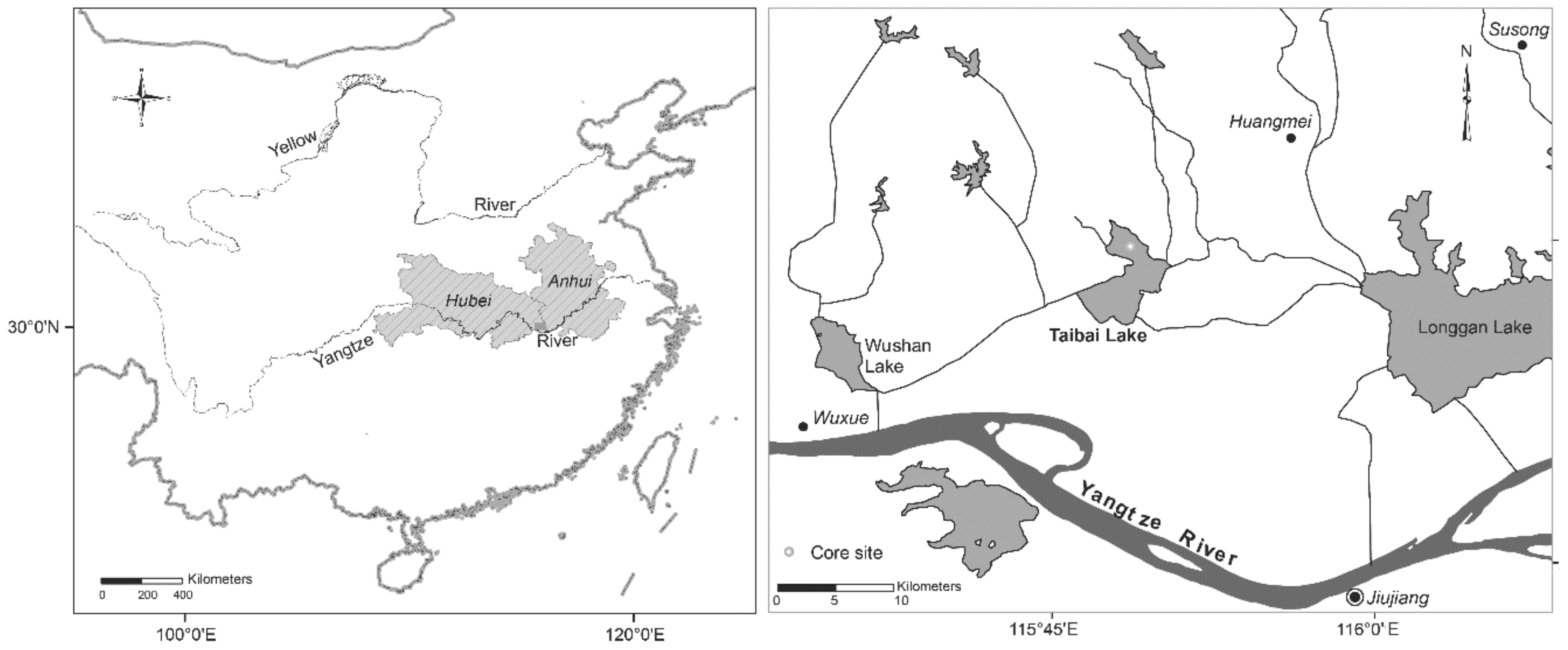
2.1. Lake and Catchment History

Taibai Lake (29°56′ to 30°01′ N, 115°46′ to 115°51′ E, 16.0 m a.s.l.) covers an area of 25.1 km2 within a 960.0 km2 catchment. It is a shallow lake, with a maximum depth of 3.9 m and an average depth of 3.2 m, which has been eutrophic approximately since 2000 [27]. Human activities and environmental changes were retrieved from historical and paleolimnological records (Table 1). Nutrient loading from chemical fertilizer application of catchment farmland, intensive aquaculture, and untreated sewage has changed slowly. Anthropogenic activities within the Taibai catchment (damming, sluices, hydroelectricity, land reclamation, and restoration) act as threshold triggers, having influenced the hydrology. The change in the function of the lake to intensive fishing and aquaculture resulted from the adoption of modifications to the social system.

2.2. Paleolimnology Reconstruction

Diatom (Class Bacillariophyceae) species are abundant, diverse, and important components in freshwater lake ecosystems and have specific habitats in a broad spectrum of conditions [33]. Subfossil diatom assemblages are often used for indicating the past environmental and ecological changes in aquatic ecosystems, including changes of water quality, nutrient status, salinity, hydrology, macrophyte cover, and food-web structure [34]. The microscopic siliceous frustules are generally well preserved in sediments and allow morphological identification to genus or species level. Therefore, subfossil diatoms are used as an ideal indicator of ecosystem states in this study.
An 83.5 cm long preliminary core TN2007 (Taibai North) was recovered using a Kajak gravity corer in 2007 at a water depth of 1.5 m from the northern center of Taibai (29°59′44.3″ N, 15°48′26.5″ E). The TN2007 core was sampled at 0.5 cm intervals from 0 to 20 cm depth and at 1.0 cm intervals from 20 to 83.5 cm depth for diatom analysis. The samples were dated using 210Pb and 137Cs radionuclide techniques with High-Purity Germanium (HPGe) Gamma Spectrometer and the constant rate of supply (CRS) model [35]. In the laboratory, sediments were digested in a water bath with 30% H2O2 and 10% HCl [33], and cleaned subsamples were dried onto coverslips and mounted onto microscope slides. At least 300 diatom valves were counted in each subsample under a light microscope with an oil immersion objective (magnification ×1000) using phase-contrast optics. Diatom taxonomy followed Krammer and Lange-Bertalot [36]. All diatom data are calculated as relative percent abundances, and taxa with abundance less than 2% of the total were excluded in the statistical analysis. The diatom diagram was drawn using the package tidypalaeo in R program, and the zones were identified using both the constrained incremental sum of squares (CONISS) and the broken-stick model [37] in R.
We used diatom species as sensitive indicators of environmental change due to the diverse biotopes of freshwater diatoms [38,39]. For example, the abundance of planktonic Aulacoseira granulata is closely correlated to the connection between a water body and its mainstream, as it has a relatively high sinking rate and requires high turbulence to maintain position in the water [40]. Changes in diatom composition have been shown to represent well the structural changes of lake primary producers [16,26].
Grain size in both cores was measured using a Malvern automated laser-optical particle-size analyzer (Mastersizer−2000; Malvern Instruments Ltd., Worcestershire, UK) after removing organic matter by 30% H2O2 treatment. Total organic carbon (TOC) content testing utilized a CE-440 elemental analyzer (EAI Exerter Analytical Inc., North Chelmsford, MA, USA) after treating 0.5 g dry samples with 5% hydrochloric acid (HCl acid). The relationship between grain size of lake sediments and critical shear stress [41] has been used as an indicator of river discharge to a lake [42,43]. Grain size also correlates robustly with paleohydrological change in nearby Longgan Lake [44]; thus, we used an index of grain size to identify hydrological differences before and after damming and sluice construction.
The catchment is known to have had excessive fertilizer applications to agricultural fields [45], suggesting that records of increasing agricultural fertilizers could semi-quantitatively represent surplus nutrient loading (Supplementary Material 1.1). Fish production biomass by Taibai from 1964 to 2013 was taken as an indicator of aquaculture intensity.

2.3. Statistical Analysis

To reduce the complexity of data, Principal Component Analysis (PCA) was applied to the relative abundance of diatom species, and the first principal component (PC1) and the second principal component (PC2) were calculated and compared to determine an indicator of variation in the diatom assemblages. Statistical methods for detecting breakpoints included sequential t-test and F-test (Chow test). We used the sequential t-test algorithm provided as an Excel add-in by Rodionov [46] for monitoring regime shifts. The algorithm requires input thresholds of regime length l and probability level p, and returns lengths of stable periods, Regime Shift Index (RSI), and mean values of stable states. In this study, we set l = 5 samples and p = 0.05. We also tested for major discontinuities with a Chow test from 15% of the whole 86 observations (with 23 interpolated data of PC1) and estimated structural changes in the regression relationship in the R package Strucchange [47]. The thresholds of the ecological state indicated by PC1 of the diatom community composition could thus be revealed in the results of the above detections.
For exploring the discontinuity in the relationships between ecological responses and main stressors, we also applied linear and breakpoint regression analyses on the combinations of diatom assemblage composition, grain size, fertilizer application, and fish production to compare magnitudes of the coefficient of determination R2 between linear fitting and step-change alternatives. Due to the constraints of available data, proxies were used to infer the strengths of stressors. The hydrodynamic state was estimated by the paleo-record of grain size. Nutrient loading and aquaculture intensity were approximated by historical records of N-P-K fertilizer application within the Hubei province and fish production. As the breakpoints were not specified in advance, structural changes were detected using the breakpoints function in the Strucchange package. The number of breaks was set as 1. To assess the relationships between system states and single dominant factors, we fitted data to two alternative patterns of response: gradual change and abrupt transition. The R2 values allowed us to compare the robustness of fitting, and the p-values were listed for comparison. The R code is available as Supplementary Material 2.

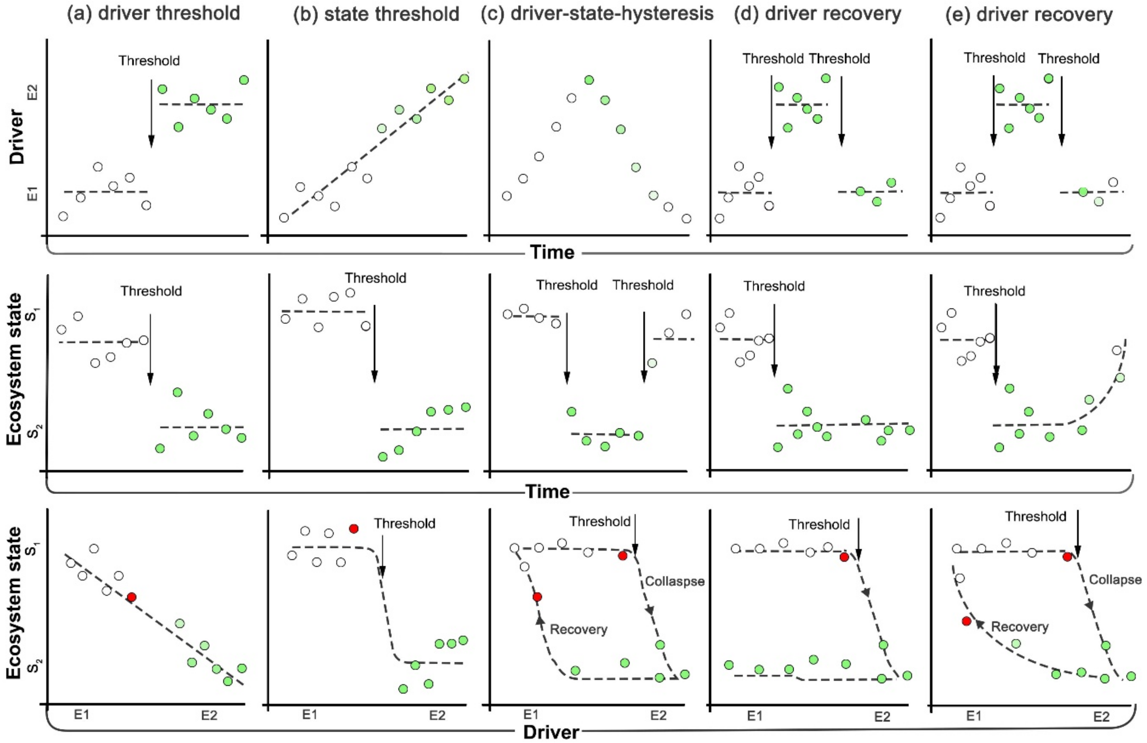
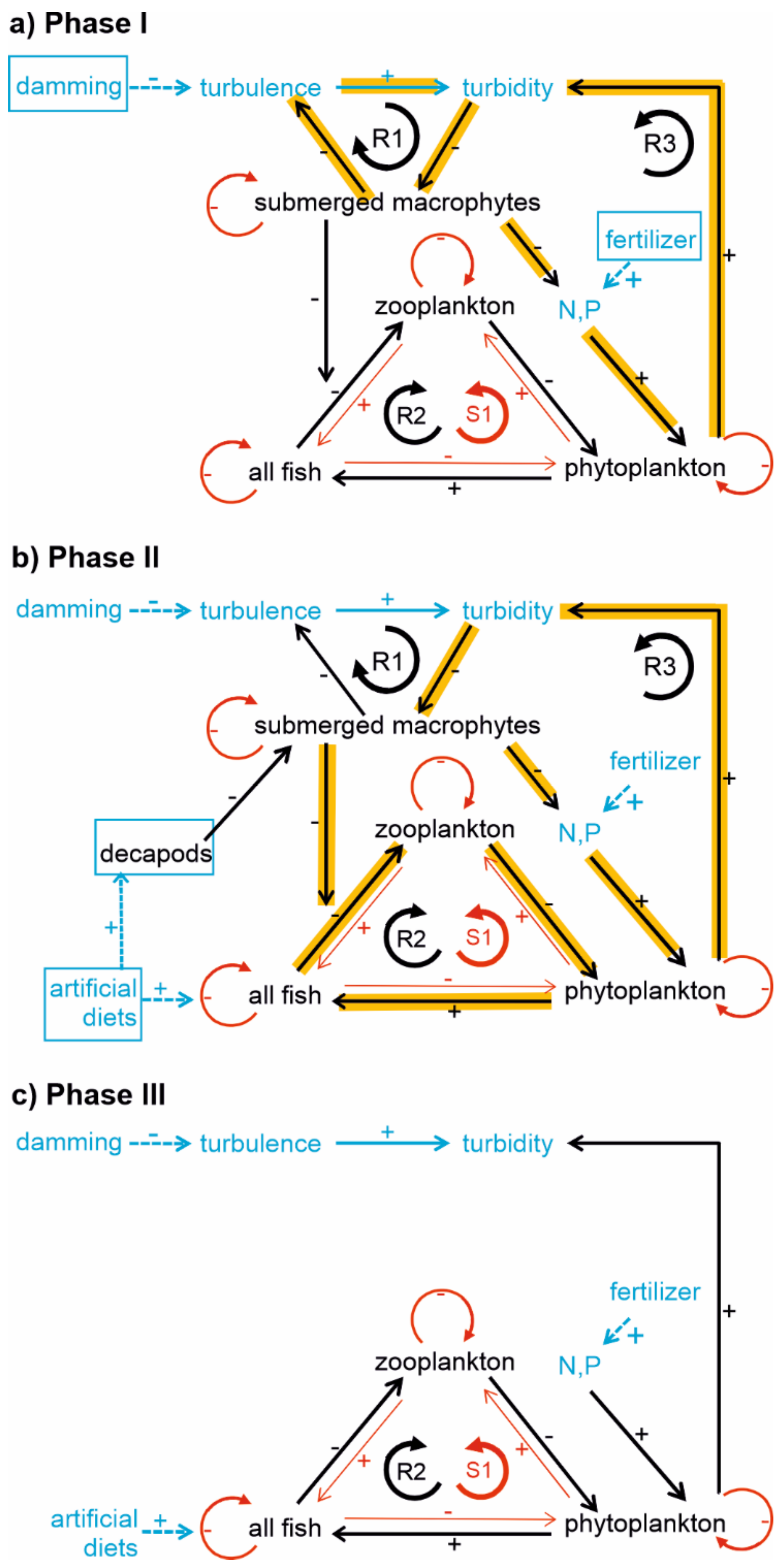
2.4. Diagrams of Interactions and Feedback Loops

In an ecosystem, there are various types of feedback mechanisms defined in terms of ecological process, length, and strength. For example, positive feedback between two components can be predator–prey interaction, facilitative interactions between species or species and its environment, and density-dependent demographic processes [48]. In trophic networks, positive 3-link feedback loops are the elementary destabilizing force balanced by the stabilizing feedback from 2-link loops and self-damping [21]. Interaction strengths are closely related to the speed of energy or biomass flow in ecological processes [49]. In a system of n components comprising feedback of various lengths, the total intensity of feedback loops is a summation of the strengths of all combinations of non-overlapping feedback loops from self-damping to n-link feedbacks.
In shallow-lake ecosystems, submerged-macrophyte-centered interactions [5,50] are widely accepted as the key functional relationships. Based on this network, we built up the dynamic interactions in Taibai’s ecosystem that create functioning positive feedback loops. Three abiotic elements, i.e., turbulence, turbidity, and nutrients, and five biotic elements, i.e., phytoplankton, zooplankton, submerged macrophytes, decapods, and fishes, were selected, as they have played important roles in ecological processes according to available records. We also identified the most important external drivers as damming, fertilizer applications in the catchment, and the use of artificial fish food. Functional positive feedbacks and effects were assessed for several periods. Following the conceptual model of feedback loops, we created a sequence of causal loop diagrams to help visualize the destabilizing processes that occur before regime shifts (Supplementary Material 1.2).

3. Results

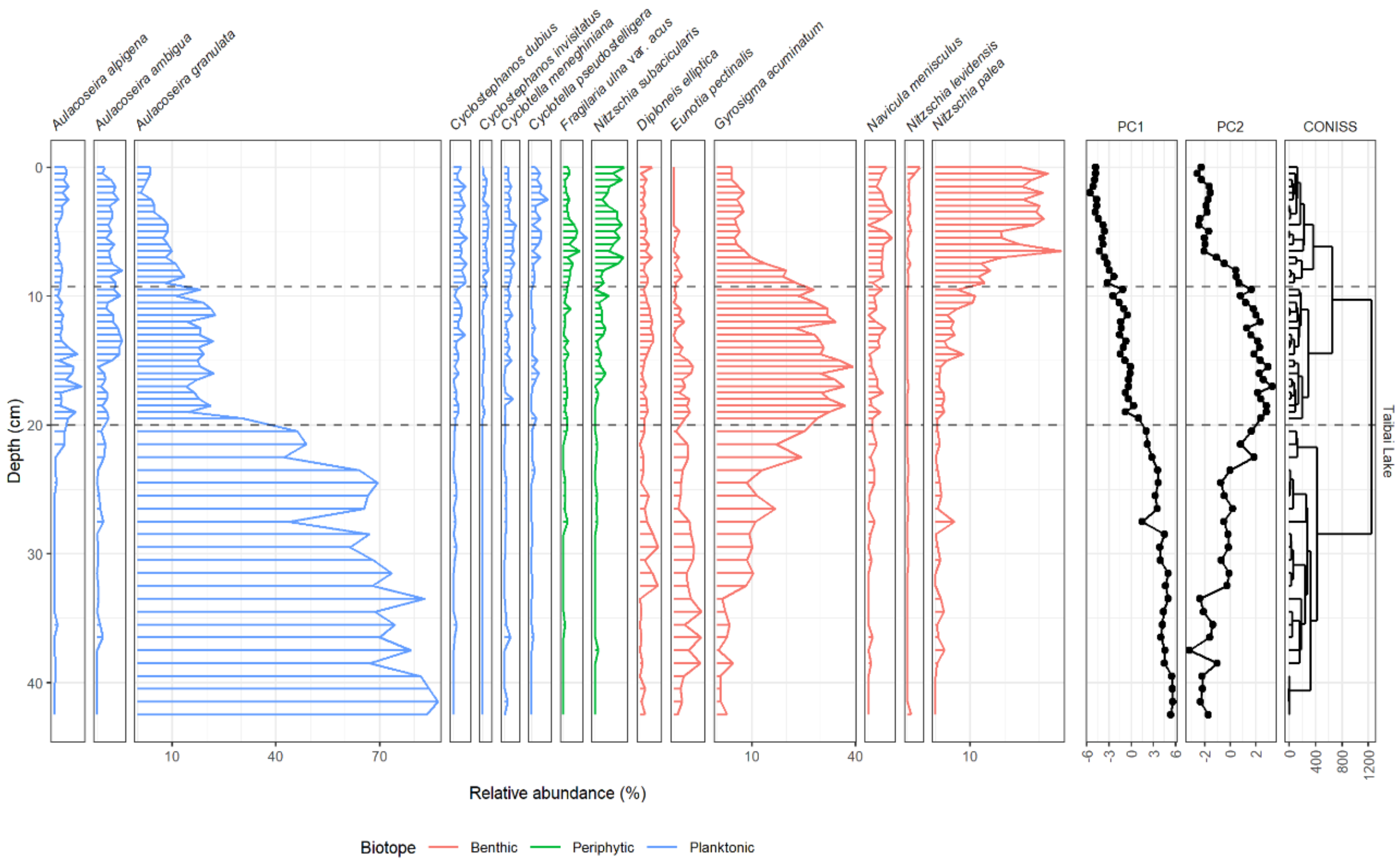
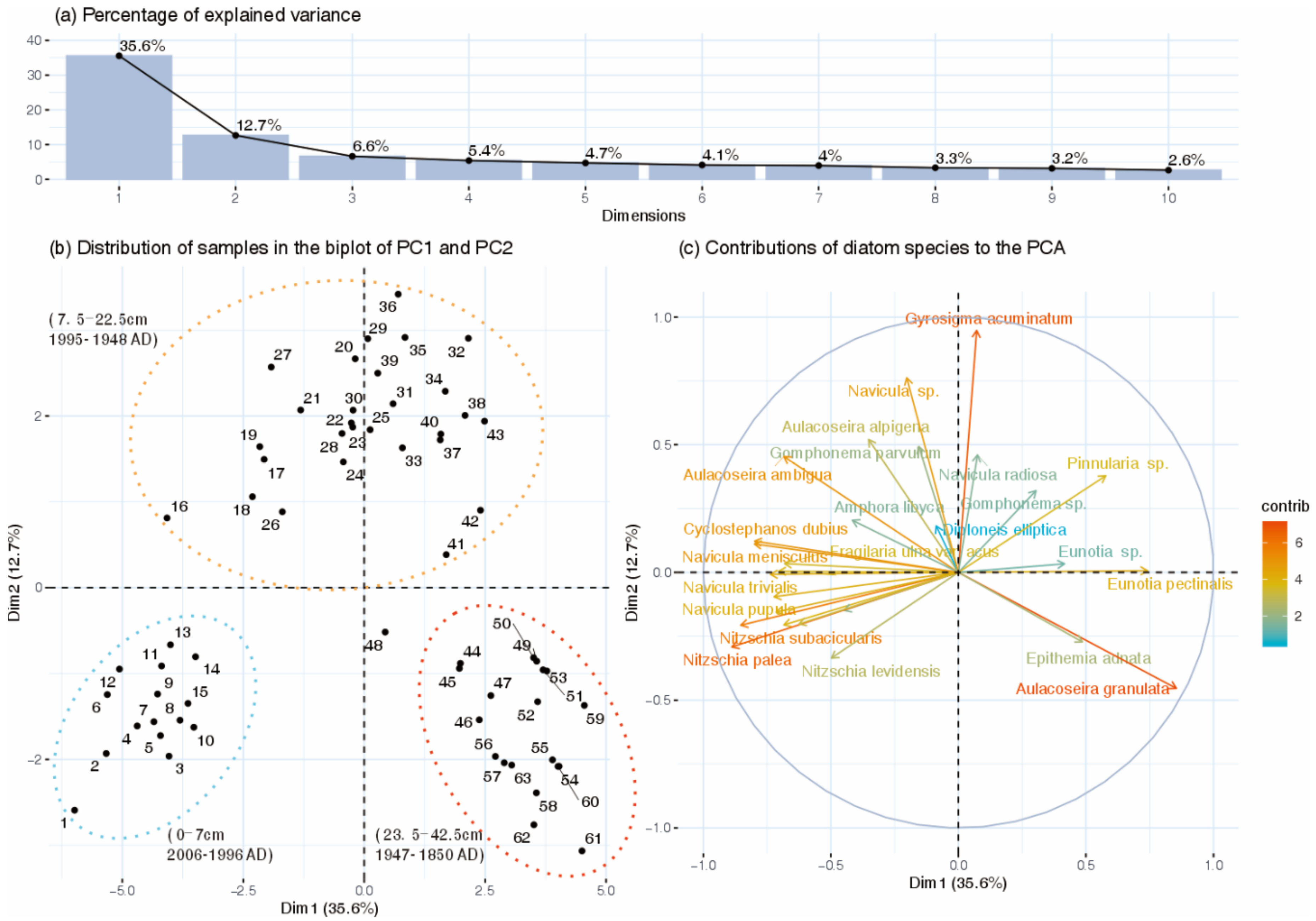
3.1. Changes in Diatom Assemblage Composition

The Taibai Lake has undergone major changes in diatom assemblages, with a general shift toward a higher relative abundance of both the periphytic Fragilaria ulna var. acus and Nitzschia subacicularis and the benthic Nitzschia palea and Navicula menisculus and a decrease in the relative abundance of planktonic Aulacoseira taxa (A. alpigena, A. ambigua and A. granulata). Here, we present the more common diatom taxa in biotope groups, and three diatom assemblage zones were identified according to the relative abundance of the taxa and cluster analysis (Figure 3). The depth data of samples are used as the vertical axis.
The bottom zone (42.5–20 cm) was dominated by the heavily silicified planktonic A. granulata and the benthic Gyrosigma acuminatum. In this interval, A. granulata gradually declined (75–45%), and benthic species increased (mainly G. acuminatum). In the middle zone (19.5–10 cm), the diatom flora was dominated by benthic taxa G. acuminatum (30–38%), while A. granulata declined dramatically at 19.5 cm from 45% to ~20%. Concurrently, the relative abundance of periphytic N. subacicularis and small planktonic A. alpigena and A. ambigua increased. The top zone (9.5–0 cm) was characterized by dominance of benthic N. palea and periphytic taxa (F. ulna var. acus and N. subacicularis). In this interval, both A. granulata and G. acuminatum decreased to under 10% relative percent abundance. The boundaries of the zones are dated at 1956 AD (19.5 cm) and 1991 AD (9.5 cm) according to the depth-age data using the 210Pb-CRS model corrected by the 137Cs 1963 peak [24].
In the result of PCA shown in Figure 4, the first and second principal components explain 35.6% and 12.7% of the total variance, respectively. The PCA axis 1 sample scores therefore can be used as an indicator of major variation in the diatom assemblage composition. The trend of PC1 declined gradually along the core, and PC2 changed in a similar way to the variation of the relative abundance of G. acuminatum, which was explained by the contributions of diatom species (Figure 4c). In the biplot of the first two components, samples fell into three clusters: 2006–1996, 1996–1948, and 1947–1850.

3.2. Tests for Ecological Thresholds

Statistical tests of tipping points on PC1 of diatom assemblages were conducted in depths for the convenience of even intervals and interpreted to date when plotting (Figure 5). In the analysis of the Breakpoints function, the linear regression model found four breakpoints in 7.0 cm, 14.0 cm, 20.0 cm, and 28.0 cm in depth, which can be inferred as 1996, 1974, 1956, and 1934. For the F statistics, sup.F = 279.97, p-value < 2.2 × 10⁻¹⁶; ave.F = 131.19, p-value < 2.2 × 10⁻¹⁶. The highest confidence of F statistics appears at 13.5 cm in depth, which means 1977. In the STARS t-test method, regime shifts were detected at 8.0 cm, 14.0 cm, 21.0 cm, and 28.5 cm in depth, which can be inferred as 1994, 1974, 1952, and 1931 in year, respectively. The parameters used in the analysis are sig= 0.05, cut-off length = 10, and Huber’s parameter =1. The regime shifts index in 1994 is higher than other three, and the RSI in 1952 is the lowest. In summary, the possible tipping points are 1994–1996, 1974–1977, 1952–1956, and 1931–1934.
The empirical relationships between environmental drivers and ecosystem states were tested and plotted in a linear regression model and breakpoint regression model (Table 2, Figure 6). In each plot, the model with a higher R2 value is colored in blue (linear regression) or red (step-change), with the alternative model shown in grey. Comparing the R squares, the values of step functions are greater in hydrodynamic and aquacultural factors. Despite higher explanatory powers, the p-values of step functions are all larger than 0.1, while linear regression models all show significance with Pr(>|t|) <0.001.

4. Discussion

4.1. Classification of Regime Shifts and Driver-Response Interactions

The driver-state interactions are envisioned straightforwardly with the help of regression models (Figure 6). When the driver-threshold transition is mediated by large and abrupt changes in hydrodynamics, the process is postulated as a driver threshold type. After 1977, the nutrient loading and intensive aquaculture affected the ecosystem slowly and progressively, helping to change the state-driver response and the shift thresholds, which is consistent with the state threshold type. Recovery scenarios in the framework (Figure 1c–e) were not examined in the Taibai data because none of the ecosystem state and nominal drivers show reversed trends over the last century. This is a widely occurring situation for disturbed Chinese shallow lakes in MLYB that have not been engineered or manipulated to improve water quality [27,51].
There are difficulties in using statistical approaches to testing for criteria related to the flexible definition of regime shift, and hypothesis-testing errors may happen due to random fluctuation induced by intervention events or missing variables due to lack of records [18]. Five step-change points were detected by t-test, but only the most significant two were accepted because they have comparatively persistent stable states, and the shifts were more distinctive than the other three. Statistical tests were therefore suitable for exploratory examination of empirical data or samples, but a regime shift needs to be confirmed using more ecological reasoning.

4.2. Feedback Loops Illustrating Regime Shifts

Functional feedbacks with the potential to actively shape the ecological threshold of regime shifts are integrated into the causal-loop diagram. There are self-damping effects in the populations, negative two-link feedback loops in trophic networks, two sets of positive three-link feedback loops (“R1” and “R2”), and positive four-link feedback loop “R3”. The other positive four-link loop between submerged macrophytes, zooplankton, phytoplankton, and turbidity is not annotated because macrophytes reduce the negative effect of fish predating zooplankton, and the process relying on predation makes the whole loop weaker than others. Nonetheless, “R1” is a self-reinforcing process between vegetation, turbulence, and turbidity and has only a single direction due to the relation between turbulence and turbidity. The “R2” describes the base of aquatic food webs between phytoplankton, zooplankton, and fish, where the combination of them should be negative in equilibrium states. The “R3” circulates among four components, i.e., nutrients, submerged macrophytes, fish, and phytoplankton, making weak positive feedback. All the positive feedbacks in Taibai’s ecosystem serve to amplify external disturbances, which are mainly linked to human activities in the last century.
We further interpreted the conceptual model to analyze dynamic changes over time (Figure 7). Pre-1950s Taibai is recorded to have strong connections to the Yangtze River, shown by the record of the median diameter of grain size at a markedly higher level. A natural wild fish community associated with the Yangtze River dominated the lake community (Table 1).
Phase I: Around 1956, an initial change occurred through damming, which greatly reduced turbulence. Nutrient runoff from increasing fertilizer usage started to couple with the effect of reduced turbidity and led to an increase in “R3”. The increased nutrients benefitted the phytoplankton, while the reduced turbidity led to an increase in submerged macrophytes and a reduction in sediment nutrients. The reconstructed biogeochemical indicator of total organic carbon increased after 1956, showing an increase in biological production.
Phase II: Additional external drivers, i.e., decapods culture and artificial fish food, modified the trophic networks through all the positive feedback. Herbivorous decapods and grass carp were introduced to reduce the submerged macrophytes, and this effect was reinforced through “R1” and “R3”. Villagers added artificial food for carp and decapods on the premise that the dietary demands of the fish exceeded the primary production of the lake (Table 1). Planktivorous fish were introduced, which amplified the initial changes in “R2”, boosting phytoplankton and reducing zooplankton, as the negative feedbacks constraining “R2” were weakened, i.e., self-damping of fish and zooplankton. As a result, the decrease of zooplankton and increase of phytoplankton were reinforced. The decreasing submerged macrophytes and increasing phytoplankton thus amplified each other in “R2” and “R3” to greatly threaten the key components of submerged macrophytes.
Phase III: In the late 1990s, records show that submerged macrophytes nearly disappeared. The linked feedbacks were gone, and only “R2” remained as positive feedback in the key relationships. The overall reinforcing effect became weaker but still destabilized the new equilibrium increasing phytoplankton. With human aquaculture interventions, the three-link feedback loops between fish, zooplankton, and phytoplankton probably remain as a weak positive loop.

4.3. Policy Implications

As confirmed in our study, regime shifts in many modern ecosystems are driven by human actions that tend to make them simpler and more homogenized with lower biodiversity and environmental quality [9]. Another tendency is the disturbance of negative feedbacks allowing positive feedback to take control of the ecosystem. Understanding the role of human impacts on regime shifts is therefore important to ecosystem management and studies. The work in Taibai achieves this goal from two aspects. First, the new case studies add to the growing number of identified regime shifts in centralized databases, e.g., the Regime Shift Database [52]: a knowledge base that can be viewed through the lens of theory to help policy making. In our study, hydrological change, nutrient loading, and aquacultural interference are factors that changed the ecosystem structure and led to abrupt transition, which should apply to similar cases in MLYB lakes. Second, providing a historical perspective for local ecological regime shifts in this way focuses attention on the longer-term impacts of specific policy and trade-offs. The early lake was an ecosystem of greater natural biodiversity and amenity than exists today. However, local society exploited the lake’s function to provide economic gain through small-scale hydroelectric power, fish farming, and nutrient-rich river runoff [25]. Future efforts to raise the natural capital of the lake will be challenging if the economic gains are to continue.
Therefore, Taibai, as an example of riverine shallow lakes in MLYB, reveals the problems of human actions on regional lake ecosystems and highlights the external forces that can push the lake ecosystems across the threshold. As the Chinese government and local governments move forward with more environmentally aware policies to promote the protection of the Yangtze River and lakes in its basin [53], the issue is how to restore the ecosystems with the experience and understanding we learned from the deterioration. The current responses to the ecological degradation of shallow lakes in the MLYB consist of reduction of nutrient levels in the watershed and extensive plantations of submerged vegetation within the lakes. In addition, all lakes along the Yangtze River have implemented a fishing ban policy from 2020 for at least ten years [53]. The effectiveness of these policies has been widely debated. For example, the effective removal of nutrients in lakes and the ecological effects of different techniques to reduce nutrient levels are still unclear and require more monitoring data [54] and synthetic analyses [55]. In practice, restoring macrophytes in large floodplain lakes may be hindered by large seasonal fluctuations of water levels [25]. The long-term fishing ban could alter the body sizes of zooplankton and thus modify the sizes and species of algae without changing the number of population [56] and prevent macrophytes from recovery due to more herbivorous fish grazing on plants. The approach used in this paper takes the relationships between the various parts of the ecosystem into account from a feedback perspective, illustrating the different patterns of ecosystem state response. The inferred feedback scenarios under external pressure provide managers a visual system-level reference.

5. Conclusions

Under the framework of hypothetical driver-response relationships containing regime shifts, ecosystem states and major drivers in Taibai since the mid-20th century were statistically tested. The results show potential ecological regime shifts in 1994–1996, 1974–1977, 1952–1956, and 1931–1934. According to R2, the relationship between the hydrodynamic factor and ecosystem states indicated by PC1 of diatom composition better fits breakpoint regression (R2 = 0.602), while the linear regression was a more suitable model for explaining the hypothetic dependence of ecosystem states on the nutrient-loading factor (R2 = 0.777). The relationship between the aquacultural factor and ecosystem states fits breakpoint regression (R2 = 0.706). The p-values are all higher than 0.1 in breakpoint regressions, indicating that these models using single factors are perhaps insufficient despite high R squares. Reconstruction of feedback mechanisms in three phases is summarized for the ecosystem states of Taibai Lake in the 1950s–1977, 1977–1990s, and post–1990s. Taibai had a fast hydraulic retention time and turbulent flow before the 1950s. After the 1950s, the interference of hydrological engineering drove the ecosystem into an alternative state with dominant positive feedback, where longer retention time and less suspended sediment helped to increase water transparency and allow submerged macrophytes to flourish and, in turn, allowed submerged macrophytes to stabilize sediments and enhance transparency. Since 1977, massive human intervention in the fish community has made impacts on both environmental variables and ecosystem state, leading to the state-threshold regime shift with, as shown in the diatom record, no indication of an instant state transition following the interventions. The patterns of state-drivers response in lake ecosystems are different due to varying feedback mechanisms and system structure, which should be considered for effective management strategies.

Supplementary Materials

The following supporting information can be downloaded at: https://www.mdpi.com/article/10.3390/w14071136/s1, Supplementary 1.1: “History of Taibai lake”; Supplementary 1.2: “Feedback loop construction”, Supplementary 2: “R code of model fitting” [5,24,28,32,57,58,59,60,61,62].

Author Contributions

Conceptualization, Y.Z., J.A.D., P.L., R.W.; methodology, Y.Z., R.W. and P.C.D.; formal analysis, Y.Z.; investigation, Y.Z. and X.Y.; data curation, Y.Z. and X.D.; writing—original draft preparation, Y.Z.; writing—review and editing, Y.Z., J.A.D., P.L., P.C.D.; visualization, Y.Z.; supervision, X.Y. and J.A.D.; funding acquisition, X.Y. and X.D. All authors have read and agreed to the published version of the manuscript.

Funding

This research was supported by National Natural Science Foundation of China (42171161), National Key R&D Program of China (2017YFA0605203), and by National Natural Science Foundation of China (41772372). The APC was funded by the Youth Innovation Promotion Association of the Chinese Academy of Sciences (award Y2021086).

Institutional Review Board Statement

Not applicable.

Informed Consent Statement

Not applicable.

Data Availability Statement

Contact the correspondence author for data.

Acknowledgments

This work was supported by the National Key R&D Program of China (2017YFA0605203) and the National Natural Science Foundation of China (No. 41772372). Y.Z. gratefully acknowledges financial support from the Chinese Scholarship Council and the University of Southampton for her Ph.D. program when the paper can be written and submitted for publication. We thank Lingyang Kong, Min Xu, and Qinghui Zhang for fieldwork and laboratory assistance, Weilan Xia for the 210Pb and 137Cs radionuclide measurement, Enfeng Liu for TN2007 radionuclide data, and Peter G. Appleby for providing the 210Pb and 137Cs dating report and for interpretative insights.

Conflicts of Interest

The authors declare no conflict of interest.

References

  1. Reynaud, A.; Lanzanova, D. A Global Meta-Analysis of the Value of Ecosystem Services Provided by Lakes. Ecol. Econ. 2017, 137, 184–194. [Google Scholar] [CrossRef] [PubMed]
  2. Schallenberg, M.; de Winton, M.D.; Verburg, P.; Kelly, D.J.; Hamill, K.D.; Hamilton, D.P. Ecosystem Services of Lakes. In Ecosystem Services in New Zealand—Conditions and Trends; Dymond, J.R., Ed.; Manaaki Whenua Press: Lincoln, New Zealand, 2013; pp. 203–225. [Google Scholar]
  3. Scheffer, M.; Carpenter, S.; Foley, J.A.; Folke, C.; Walker, B.R. Catastrophic shifts in ecosystems. Nature 2001, 413, 591–596. [Google Scholar] [CrossRef] [PubMed]
  4. Schindler, D.W. The dilemma of controlling cultural eutrophication of lakes. Proc. R. Soc. B 2012, 279, 4322–4333. [Google Scholar] [CrossRef] [PubMed] [Green Version]
  5. Scheffer, M.; Hosper, S.H.; Meijer, M.-L.; Moss, B.; Jeppesen, E. Alternative equilibria in shallow lakes. Trends Ecol. Evol. 1993, 8, 275–279. [Google Scholar] [CrossRef]
  6. Qin, B.Q.; Gao, G.; Zhu, G.W.; Zhang, Y.L.; Song, Y.Z.; Tang, X.M.; Xu, H.; Deng, J.M. Lake eutrophication and its ecosystem response. Chin. Sci. Bull. 2013, 58, 961–970. [Google Scholar] [CrossRef] [Green Version]
  7. Rockström, J.; Steffen, W.; Noone, K.; Persson, Å.; Chapin, F.S., III; Lambin, E.F.; Lenton, T.M.; Scheffer, M.; Folke, C.; Schellnhuber, H.J.; et al. A safe operating space for humanity. Nature 2009, 461, 472–475. [Google Scholar] [CrossRef]
  8. Scheffer, M.; Carpenter, S.R. Catastrophic regime shifts in ecosystems: Linking theory to observation. Trends Ecol. Evol. 2003, 18, 648–656. [Google Scholar] [CrossRef]
  9. Folke, C.; Carpenter, S.; Walker, B.; Scheffer, M.; Elmqvist, T.; Gunderson, L.; Holling, C.S. Regime shifts, resilience, and biodiversity in ecosystem management. Annu. Rev. Ecol. Evol. Syst. 2004, 35, 557–581. [Google Scholar] [CrossRef] [Green Version]
  10. Kong, X.; He, Q.; Yang, B.; He, W.; Xu, F.; Janssen, A.B.G.; Kuiper, J.J.; van Gerven, L.P.A.; Qin, N.; Jiang, Y.; et al. Hydrological regulation drives regime shifts: Evidence from palaeolimnology and ecosystem modeling of a large shallow Chinese lake. Glob. Chang. Biol. 2017, 23, 737–754. [Google Scholar] [CrossRef]
  11. Kuehn, C. A mathematical framework for critical transitions: Bifurcations, fast–slow systems and stochastic dynamics. Phys. D Nonlinear Phenom. 2011, 240, 1020–1035. [Google Scholar] [CrossRef] [Green Version]
  12. Veraart, A.J.; Faassen, E.J.; Dakos, V.; Van Nes, E.H.; Lürling, M.; Scheffer, M. Erratum: Corrigendum: Recovery rates reflect distance to a tipping point in a living system. Nature 2012, 484, 404. [Google Scholar] [CrossRef] [Green Version]
  13. Carpenter, S.R.; Cole, J.J.; Pace, M.L.; Batt, R.; Brock, W.A.; Cline, T.; Coloso, J.; Hodgson, J.R.; Kitchell, J.F.; Seekell, D.A.; et al. Early Warnings of Regime Shifts: A Whole-Ecosystem Experiment. Science 2011, 332, 1079–1082. [Google Scholar] [CrossRef] [Green Version]
  14. Seekell, D.A.; Cline, T.J.; Carpenter, S.R.; Pace, M.L. Evidence of alternate attractors from a whole-ecosystem regime shift experiment. Theor. Ecol. 2013, 6, 385–394. [Google Scholar] [CrossRef] [Green Version]
  15. Søndergaard, M.; Lauridsen, T.L.; Johansson, L.S.; Jeppesen, E. Repeated Fish Removal to Restore Lakes: Case Study of Lake Væng, Denmark—Two Biomanipulations during 30 Years of Monitoring. Water 2017, 9, 43. [Google Scholar] [CrossRef] [Green Version]
  16. Doncaster, C.P.; Chávez, V.A.; Viguier, C.; Wang, R.; Zhang, E.; Dong, X.; Dearing, J.; Langdon, P.; Dyke, J.G. Early warning of critical transitions in biodiversity from compositional disorder. Ecology 2016, 97, 3079–3090. [Google Scholar] [CrossRef]
  17. Wang, R.; Dearing, J.A.; Langdon, P.G.; Zhang, E.; Yang, X.; Dakos, V.; Scheffer, M. Flickering gives early warning signals of a critical transition to a eutrophic lake state. Nature 2012, 492, 419–422. [Google Scholar] [CrossRef]
  18. Andersen, T.; Carstensen, J.; Hernandez-Garcia, E.; Duarte, C.M. Ecological thresholds and regime shifts: Approaches to identification. Trends Ecol. Evol. 2009, 24, 49–57. [Google Scholar] [CrossRef] [Green Version]
  19. Jeppesen, E.; Appelt, M.; Hastrup, K.; Grønnow, B.; Mosbech, A.; Smol, J.P.; Davidson, T.A. Living in an oasis: Rapid transformations, resilience, and resistance in the North Water Area societies and ecosystems. AMBIO 2018, 47, 296–309. [Google Scholar] [CrossRef] [Green Version]
  20. Patten, B.C. Ecosystem Linearization: An Evolutionary Design Problem. Am. Nat. 1975, 109, 529–539. [Google Scholar] [CrossRef]
  21. Neutel, A.; Thorne, M. Interaction strengths in balanced carbon cycles and the absence of a relation between ecosystem complexity and stability. Ecol. Lett. 2014, 17, 651–661. [Google Scholar] [CrossRef] [Green Version]
  22. Kéfi, S.; Holmgren, M.; Scheffer, M. When can positive interactions cause alternative stable states in ecosystems? Funct. Ecol. 2015, 30, 88–97. [Google Scholar] [CrossRef]
  23. Scheffer, M.; Carpenter, S.R.; Lenton, T.M.; Bascompte, J.; Brock, W.; Dakos, V.; van de Koppel, J.; van de Leemput, I.A.; Levin, S.A.; van Nes, E.H.; et al. Anticipating Critical Transitions. Science 2012, 338, 344–348. [Google Scholar] [CrossRef] [Green Version]
  24. Liu, Q.; Yang, X.; Anderson, J.; Liu, E. Diatom ecological response to altered hydrological forcing of a shallow lake on the Yangtze floodplain, SE China. Ecohydrology 2012, 268, 256–268. [Google Scholar] [CrossRef]
  25. Xu, M.; Dong, X.; Yang, X.; Chen, X.; Zhang, Q.; Liu, Q.; Wang, R.; Yao, M.; Davidson, T.A.; Jeppesen, E. Recent Sedimentation Rates of Shallow Lakes in the Middle and Lower Reaches of the Yangtze River: Patterns, Controlling Factors and Implications for Lake Management. Water 2017, 9, 617. [Google Scholar] [CrossRef]
  26. Wang, R.; Dearing, J.A.; Doncaster, C.P.; Yang, X.; Zhang, E.; Langdon, P.; Yang, H.; Dong, X.; Hu, Z.; Xu, M.; et al. Network parameters quantify loss of assemblage structure in human-impacted lake ecosystems. Glob. Chang. Biol. 2019, 25, 3871–3882. [Google Scholar] [CrossRef]
  27. Yang, X.; Shen, J.; Dong, X.; Liu, E.; Wang, S. Historical trophic evolutions and their ecological responses from shallow lakes in the middle and lower reaches of the Yangtze River: Case studies on Longgan Lake and Taibai Lake. Sci. China Ser. D Earth Sci. 2006, 49, 51–61. [Google Scholar] [CrossRef]
  28. Jian, Y. A comparative study of aquatic plant diversity of Haikou, Taibai and Wushan Lake in Hubei Province of China. Acta Ecol. Sin. 2001, 21, 1815–1824. [Google Scholar]
  29. Liu, E.; Yang, X.; Shen, J.; Dong, X.; Zhang, E.; Wang, S. Environmental response to climate and human impact during the last 400 years in Taibai Lake catchment, middle reach of Yangtze River, China. Sci. Total Environ. 2007, 385, 196–207. [Google Scholar] [CrossRef]
  30. Zhao, Y.; Wang, R.; Yang, X.; Dong, X.; Xu, M. Regime shifts revealed by paleoecological records in Lake Taibai’s ecosystem in the middle and lower Yangtze River Basin during the last century. J. Lake Sci. 2016, 28, 1381–1390. [Google Scholar] [CrossRef] [Green Version]
  31. Gui, J.; Tang, Q.; Li, Z.; Liu, J.; De Silva, S.S. Aquaculture in China: Success Stories and Modern Trends; Wiley-Blackwell: London, UK, 2018. [Google Scholar] [CrossRef]
  32. National Bureau of Statistics of China. Huanggang Statistical Yearbook-2010; China Statistics Press: Beijing, China, 2010.
  33. Battarbee, R.W.; Jones, V.J.; Flower, R.J.; Cameron, N.G.; Bennion, H.; Carvalho, L.; Juggins, S. Diatoms; Smol, J., Birks, H.J., Last, W., Bradley, R., Alverson, K., Eds.; Springer: Dordrecht, The Netherlands, 2005; pp. 155–202. [Google Scholar]
  34. Smol, J.P.; Stoermer, E.F. (Eds.) The Diatoms: Applications for the Environmental and Earth Sciences, 2nd ed.; Cambridge University Press: Cambridge, UK, 2010. [Google Scholar]
  35. Appleby, P. Three decades of dating recent sediments by fallout radionuclides: A review. Holocene 2008, 18, 83–93. [Google Scholar] [CrossRef]
  36. Krammer, K.; Lange-Bertalot, H. Bacillariophyceae(1-4Teil), Süßwasserflora von Mitteleuropa; Spektrum Akademischer Verlag: Heidelberg, Germany, 1999. [Google Scholar]
  37. Bennett, K. Determination of the number of zones in a biostratigraphical sequence. New Phytol. 1996, 132, 155–170. [Google Scholar] [CrossRef] [PubMed]
  38. Seckbach, J.; Kociolek, J.P. The Diatom World, Cellular Origin, Life in Extreme Habitats and Astrobiology; Springer: Dordrecht, The Netherlands, 2011. [Google Scholar] [CrossRef]
  39. Smol, J.P.; Birks, H.J.B.; Last, W.M. Tracking Environmental Change Using Lake Sediments. Volume 3, Terrestrial, Algal, and Siliceous Indicators, Developments in Palaeoenvironmental Research; Kluwer Academic: Dordrecht, The Netherlands, 2002. [Google Scholar]
  40. Reid, M.A.; Ogden, R.W. Factors affecting diatom distribution in floodplain lakes of the southeast Murray Basin, Australia and implications for palaeolimnological studies. J. Paleolimnol. 2008, 41, 453–470. [Google Scholar] [CrossRef]
  41. Dearing, J.A. Sedimentary indicators of lake-level changes in the humid temperate zone: A critical review. J. Paleolimnol. 1997, 18, 1–14. [Google Scholar] [CrossRef]
  42. Chiverrell, R.; Sear, D.; Warburton, J.; Macdonald, N.; Schillereff, D.; Dearing, J.; Croudace, I.; Brown, J.; Bradley, J. Using lake sediment archives to improve understanding of flood magnitude and frequency: Recent extreme flooding in northwest UK. Earth Surf. Process. Landforms 2019, 44, 2366–2376. [Google Scholar] [CrossRef]
  43. Dearing, J.A.; Jones, R.T.; Shen, J.; Yang, X.; Boyle, J.F.; Foster, G.C.; Crook, D.S.; Elvin, M.J.D. Using multiple archives to understand past and present climate—human-environment interactions: The lake Erhai catchment, Yunnan Province, China. J. Paleolimnol. 2008, 40, 3–31. [Google Scholar] [CrossRef]
  44. Xue, J.; Li, J.; Dang, X.; Meyers, A.P.; Huang, X. Paleohydrological changes over the last 4000 years in the middle and lower reaches of the Yangtze River: Evidence from particle size and n-alkanes from Longgan Lake. Holocene 2017, 27, 1318–1324. [Google Scholar] [CrossRef]
  45. Ju, X.T.; Xing, G.X.; Chen, X.P.; Zhang, S.L.; Zha, L.J.; Liu, X.J.; Cui, Z.L.; Yin, B.; Christie, P.; Zhu, Z.L.; et al. Reducing environmental risk by improving N management in intensive Chinese agricultural systems. Proc. Natl. Acad. Sci. USA 2009, 106, 8077. [Google Scholar] [CrossRef] [Green Version]
  46. Rodionov, S.N. A sequential algorithm for testing climate regime shifts. Geophys. Res. Lett. 2004, 31, 1–4. [Google Scholar] [CrossRef] [Green Version]
  47. Zeileis, A.; Kleiber, C.; Krämer, W.; Hornik, K. Testing and dating of structural changes in practice. Comput. Stat. Data Anal. 2003, 44, 109–123. [Google Scholar] [CrossRef] [Green Version]
  48. Van de Leemput, I.A.; Hughes, T.P.; van Nes, E.H.; Scheffer, M. Multiple feedbacks and the prevalence of alternate stable states on coral reefs. Coral Reefs 2016, 35, 857–865. [Google Scholar] [CrossRef]
  49. Rooney, N.; McCann, K.S.; Gellner, G.; Moore, J.C. Structural asymmetry and the stability of diverse food webs. Nature 2006, 442, 265–269. [Google Scholar] [CrossRef]
  50. Jeppesen, E.; Jensen, J.P.; Søndergaard, M.; Lauridsen, T.; Møller, P.H.; Sandby, K. Changes in nitrogen retention in shallow eutrophic lakes following a decline in density of cyprinids. Fundam. Appl. Limnol. 1998, 142, 129–151. [Google Scholar] [CrossRef]
  51. Qin, B.; Zhu, G. The nutrient forms, cycling and exchange flux in the sediment and overlying water system in lakes from the middle and lower reaches of Yangtze River. Sci. China Ser. D Earth Sci. 2006, 49, 1–13. [Google Scholar] [CrossRef]
  52. Biggs, R.; Peterson, G.D.; Rocha, J.C. The Regime Shifts Database: A framework for analyzing regime shifts in social-ecological systems. Ecol. Soc. 2018, 23, 9. [Google Scholar] [CrossRef]
  53. Chen, T.; Wang, Y.; Gardner, C.; Wu, F. Threats and protection policies of the aquatic biodiversity in the Yangtze River. J. Nat. Conserv. 2020, 58, 125931. [Google Scholar] [CrossRef]
  54. Xu, H.; McCarthy, M.J.; Paerl, H.W.; Brookes, J.D.; Zhu, G.; Hall, N.S.; Qin, B.; Zhang, Y.; Zhu, M.; Hampel, J.J.; et al. Contributions of external nutrient loading and internal cycling to cyanobacterial bloom dynamics in Lake Taihu, China: Implications for nutrient management. Limnol. Oceanogr. 2021, 66, 1492–1509. [Google Scholar] [CrossRef]
  55. Anderson, N.J.; Jeppesen, E.; Søndergaard, M. Ecological effects of reduced nutrient loading (oligotrophication) on lakes: An introduction. Freshw. Biol. 2005, 50, 1589–1593. [Google Scholar] [CrossRef]
  56. Brucet, S.; Tavşanoğlu, Ü.N.; Özen, A.; Levi, E.E.; Bezirci, G.; Çakıroğlu, A.I.; Jeppesen, E.; Svenning, J.-C.; Ersoy, Z.; Beklioğlu, M. Size-based interactions across trophic levels in food webs of shallow Mediterranean lakes. Freshw. Biol. 2017, 62, 1819–1830. [Google Scholar] [CrossRef]
  57. Zou, Y. Population Time Series of Longgan-Taibai Lake Catchment during 1391–2006 and its Sediment Response. J. Chin. Hist Geogr 2011, 03, 41–59. [Google Scholar]
  58. National Bureau of Statistics of China. Hubei Statistical Yearbook-2013; China Statistics Press: Beijing, China, 2013.
  59. Cao, Y.; Zhang, E.; Langdon, P.G.; Liu, E.; Shen, J. Chironomid-inferred environmental change over the past 1400 years in the shallow, eutrophic Taibai Lake (south-east China): Separating impacts of climate and human activity. Holocene 2014, 24, 581–590. [Google Scholar] [CrossRef]
  60. Scheffer, M. Ecology of Shallow Lakes. In Population and Community Biology Series; Kluwer Academic Publishers: London, UK, 1998. [Google Scholar] [CrossRef]
  61. Jeppesen, E.; Søndergaard, M.; Søndergaard, M.; Christoffersen, K. (Eds.) The Structuring Role of Submerged Macrophytes in Lakes; Springer: New York, NY, USA, 1998. [Google Scholar] [CrossRef]
  62. Meiburg, E.; Kneller, B. Turbidity currents and their deposits. Annu. Rev. Fluid Mech 2010, 42, 135–156. [Google Scholar] [CrossRef] [Green Version]
Figure 1. Conceptual models of alternative types of regime shifts and threshold transitions (ac) after Andersen et al. [18] and (d,e) after Jeppesen et al. [19]). White and green dots distinguish ecosystem states S1 and S2, respectively. Red dots identify threshold points of abrupt and persistent change in driver or ecosystem state, and arrows identify the direction of change. The three rows display the driver (top row) and ecosystem (middle row) state developing through time and the ecosystem response to the driver (bottom row) with consequences for ecosystem structure.
Water 14 01136 g001
Figure 2. Map of Taibai Lake catchment in MLYB. Left-hand map shows the middle-lower reach of Yangtze River in China, between Hubei and Anhui province (green shadow), and the location of Taibai Lake catchment (orange square). The right-hand map shows the northern central coring site in Taibai, northern reservoirs draining into the lake, and connecting rivers/canals with other lakes and the Yangtze River.
Water 14 01136 g002
Figure 3. A stratigraphic diagram of the diatom assemblages for TN2007, with the first two axes of PCA and zonations of the broken-stick model.
Water 14 01136 g003
Figure 4. Explained variance of principal components, PC-scores along the first two axes of the PCAs, and contributions of diatom species. (a) percentage of explained variance; (b) distribution of sediment samples in the PCA biplot; (c) contributions of diatom species to the total variation.
Water 14 01136 g004
Figure 5. Detected breakpoints using multiple approaches of the sequential t-test and F-test.
Water 14 01136 g005
Figure 6. Regression models of the state-driver responses in Taibai Lake. (a) Hydrodynamic Factor; (b) Nutrient Factor; (c) Aquacultural Factor.
Water 14 01136 g006
Figure 7. Diagrams of reconstructed dynamic changes in Taibai Lake in the last decades. Straight arrows show positive (+) and negative (−) interactions. New interventions are shown in blue boxes. Yellow-highlighted arrows indicate triggering forces that stimulate circular interactions. In a closed-loop, an odd number of negative interactions means a negative or stabilizing feedback loop (red arrows); an even or zero number of negative interactions means a positive or reinforcing loop (“R”, black arrows). (a) inferred feedback loops around 1956; (b) modified feedback loops from 1960s to 1990s; (c) simpler feedback loops because links related to submerged macrophytes drop out.
Water 14 01136 g007
Table 1. Human activities in Taibai during the last decades.
PeriodsHuman Activity and Paleolimnological Evidence
1970s–present2000–present: Reducing vegetation coverage [28]
2000–present: Widespread adoption of flush toilets that are unconnected with local piped sewage systems and a lack of new treatment plants have added to the increase in nutrient loading [29]
1987–present: Fish farm owners introduced economic domestic fishes into the lake, and the aquaculture intensity upgraded to a high level, resulting in exponential growth in aquaculture products [30]
1983–1993: High sedimentation flux correlated to soil loss due to intensive cultivation development [29,31]
1978–2013: In the lake catchment, the population increased and human settlements expanded, while farmland and lake area shrank (Supplementary Material 1.1) [32]
1976–present: Tongsipai Floodgate cut the dispersal route for juvenile fishes [30]
The 1950s–1980sThe 1950s–1978: Rapidly developing local industrialization, mainly chemical fertilizer factories [29]. Thereafter, the lake received more nutrient loading from increasing domestic sewage, poorly treated industrial waste, and flushed chemical fertilizer [28]
1958–1970: High sedimentation flux correlated with the land reclamation around Taibai [29]
1955–1962: Damming construction: three reservoirs named Jingzhu, Kaotian, and Xianrenba were built in the upper reaches of Taibai. The lake outflow passes through lake Longgan to the east of Taibai and drains to the Yangtze River [29]
Previous to 1950The lake had periodic direct inflow connections with the Yangtze during floods [29,30]
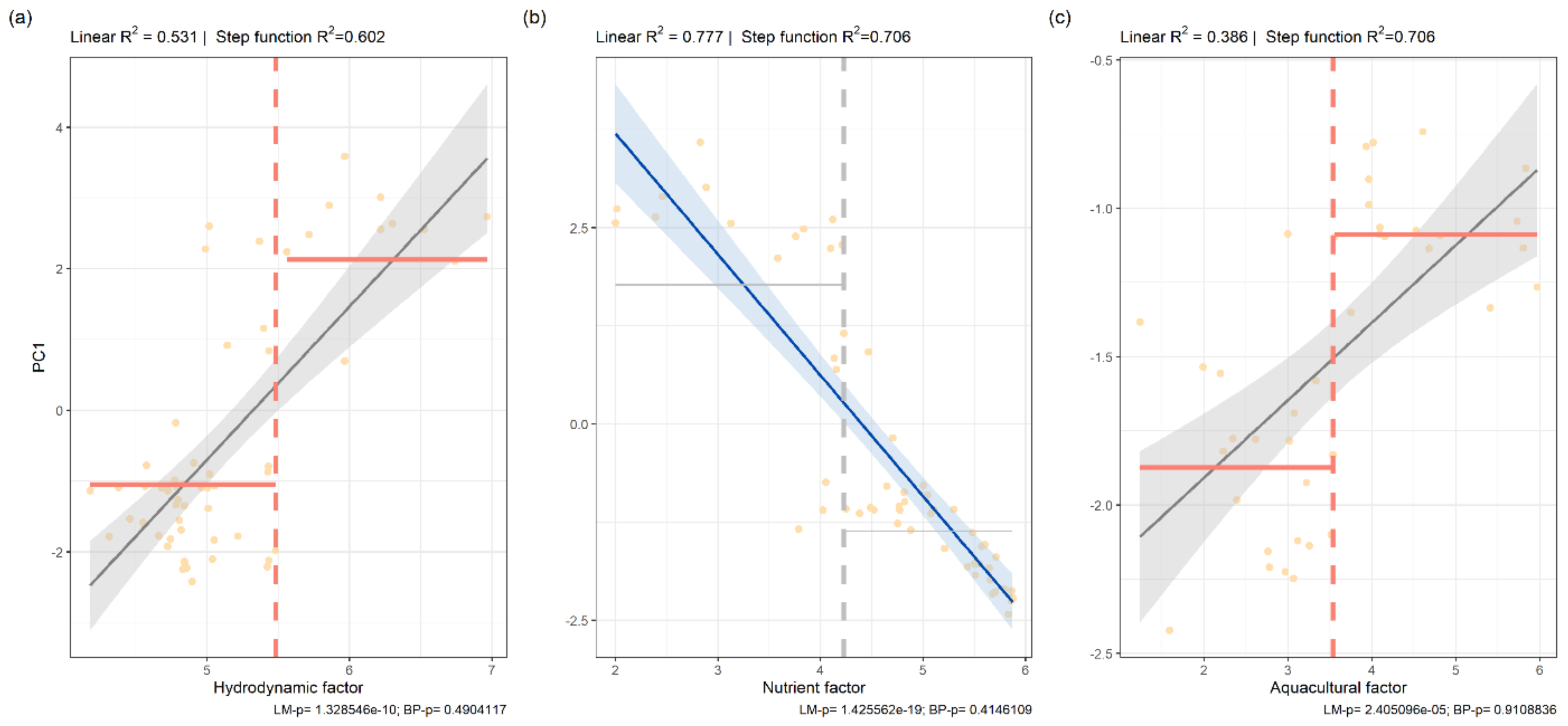
Table 2. Linear regression models containing no breakpoints between the stressors and ecological response.
Intercept ± SESlope ± SER2Pr(>|t|)F-Test of Model Fit
PC1~MD11.5268 ± 1.42512.1657 ± 0.27460.53081.33 × 10−10F (1,55) = 62.22, p < 0.001
PC1~FA6.7809 ± 0.5283−1.5404 ± 0.11120.7771<2 × 10⁻¹⁶F (1,55) = 191.8, p < 0.001
PC1~FP−2.43085 ± 0.204520.26146 ± 0.054170.38642.41 × 10−5F (1,37) = 23.3, p < 0.001
Publisher’s Note: MDPI stays neutral with regard to jurisdictional claims in published maps and institutional affiliations.

