
Numerical Investigation on Solitary Wave Interaction with a Vertical Cylinder over a Viscous Mud Bed


Department of Engineering Science and Ocean Engineering, National Taiwan University, Taipei City 10617, Taiwan
*
Author to whom correspondence should be addressed.
Water 2022, 14(7), 1135; https://doi.org/10.3390/w14071135
Submission received: 17 March 2022
/
Revised: 25 March 2022
/
Accepted: 29 March 2022
/
Published: 1 April 2022
(This article belongs to the Special Issue Research on the Interaction of Water Waves and Ocean Structures)
Abstract
:This study investigated the hydrodynamics of a solitary wave passing a vertical cylinder over a viscous mud bed for the first time. A highly viscous Newtonian fluid was assumed as a simplified model for fluid mud. A three-dimensional numerical wave flume consisting of a fixed cylindrical structure and three viscous fluids—air, water, and mud—was constructed and validated. Numerical experiments were performed to investigate solitary wave interaction with a vertical cylinder over a viscous mud bed. Numerical results showed the mud surface deformation to be one order of magnitude smaller than the water surface deformation and their behaviors to be different: mud surface depressions occurred on the upstream and downstream sides of the cylinder, whereas mud surface elevations occurred on the lateral sides of the cylinder. This solitary wave induced scour pattern on a muddy seabed is different from that commonly observed on a sandy seabed. Water flow reversal near the water–mud interface was made more evident by the mud bed. Although the mud bed attenuated water waves, it nevertheless increased the total horizontal force and toppling moment exerted on the cylinder due to the wave-induced mud flow. These findings may be valuable to the design of marine structures on a muddy seabed and worthy of further investigation.
1. Introduction
The ocean makes up at least two-thirds of the Earth’s surface. As demand for energy grows, interest in harvesting resources in the ocean follow. Nowadays, abundant research on related topics can be found (see, e.g., a series of studies introduced by Correia et al. [1]). The design and construction of marine structures remain an important and relevant topic in ocean engineering. For example, scour around the foundations of marine structures, though a classical topic, still receives tremendous research efforts due to its complexity and practical value (see, e.g., a recent review by Fazeres-Ferradosa et al. [2]).
The placement of marine structures ranges from nearshore to offshore. In a nearshore environment, water waves are an important hydrodynamic factor to consider. Long waves (or shallow water waves), whose wavelengths are significantly larger than the water depth, are commonly assumed to study long-period waves such tsunamis, infragravity waves, and typhoon-induced swells in a nearshore environment.
Due to its clear mathematical definition and easiness to replicate, solitary waves are one of the most widely used long-wave models. For example, Grimshaw [3] derived a solitary wave solution in water of variable depth. Solitary waves also see numerous applications in studies on tsunamis (transient long waves), impacts of extreme waves on marine structures, nearshore sediment transport, swash zone dynamics, etc. (see e.g., Isaacson [4], Wang et al. [5], Yates and Wang [6], Tonkin et al. [7], Mo et al. [8], Lo and Liu [9], Pujara et al. [10], Larsen et al. [11,12], and Wu et al. [13]). The leading-order solution for the free surface displacement of a solitary wave reads
in which H is the wave height, h is the still water depth, g is the gravitational acceleration, t is time, x is the horizontal spatial coordinate, and
is the wave speed. Strictly speaking, solitary waves have infinitely long wavelength. However, in practice, an effective wavelength l is often used:
To minimize wave drag in all directions, the foundation piles of marine structures usually have circular cross sections (see, e.g., Jamalabadi and Oveisi [14]). In studies on wave and current interactions with marine structures, vertical cylinders are often assumed as an approximate shape of foundation piles. For example, Isaacson [4] derived the analytical solution for solitary wave diffraction around a large cylinder; Wang et al. [5] performed numerical simulations of the same problem based on a depth-averaged wave model; Yates and Wang [6] conducted laboratory experiments on the same problem and compared the wave runup around the cylinder and the forces exerted on the cylinder with numerical results; Mo et al. [8] performed three-dimensional (3D) numerical simulations of wave–cylinder interaction for both regular waves and solitary waves, and validated the numerical results through large-scale laboratory experiments; Tonkin et al. [7] experimentally investigated tsunami-induced scour around a coastal cylindrical structure; Larsen et al. [11] numerically investigated tsunami-induced scour around a monopile structure, representative of offshore wind turbine foundations in moderate water depths; Larsen et al. [12] performed laboratory experiments on the same problem and validated the numerical results in Larsen et al. [11]; Li et al. [15] conducted 3D numerical simulations to mimic the Tonkin et al. [7] laboratory experiments; Li et al. [16] conducted 3D numerical simulations to study tsunami-induced scour around a bridge pier.
In modeling, seabeds can be loosely divided into three categories: rigid, sandy, and muddy. Conventionally, either a rigid seabed or a sandy seabed is assumed in studies on wave-structure interaction, such as the above-mentioned examples. Simply put, a rigid seabed consists of bedrock and boulders, often modeled as an impermeable solid bottom boundary. A sandy seabed consists of granular (large-grain) materials like sand and gravel, often modeled as a porous media whose pore pressure effects must be considered. As pointed out by Healy et al. [17], muddy seabeds exist in many parts of the world. While the scour of sandy seabeds has been studied extensively (see, e.g., Sumer et al. [18]), studies on the scour of muddy seabeds are scarce. A muddy seabed consists of cohesive (fine-grain) sediments such as mud and clay, whose inter-particle adhesive forces must be considered and a rheological model is often assumed. Studies have indicated that cohesive sediments demonstrate different scour and erosion characteristics from noncohesive granular materials and warrant further investigation (see, e.g., Schindler et al. [19], Harris and Whitehouse [20]). While scour protection countermeasures in uniform noncohesive soils have been widely studied (see e.g., Fazeres-Ferradosa et al. [21]), knowledge on the behavior of scour and scour protections in cohesive soils or layered noncohesive soils is lacking (see, e.g., Fazeres-Ferradosa et al. [2], Porter et al. [22]). This study seeks to improve the understanding of wave-structure interaction over a muddy seabed (i.e., cohesive sediments).
Wave–mud interaction, especially the attenuation of waves by a muddy seabed, has been studied by various researchers. As the most simplified model, the mud is commonly assumed to be a highly viscous Newtonian fluid mud. Gade [23] derived analytical solutions based on a two-fluid model, in which the upper layer is a shallow-depth inviscid fluid (water) and the lower layer is a Newtonian viscous fluid mud, and compared the results with experimental measurements. Dalrymple and Liu [24] extended the Gade [23] model to any water depth and considered the viscosity of water, and found that high wave attenuation rates are possible when the mud layer is thick or when the mud layer is about as thick as its boundary layer. By considering the water boundary layer near the water–mud interface, the mud boundary layer near the water–mud interface, and mud boundary layer near the rigid bottom, Jiang and Zhao [25] analyzed the attenuation of solitary waves propagating over a Newtonian fluid-mud seabed, and conducted laboratory experiments to validate the analytical results. Based on the Boussinesq wave model, Liu and Chan [26] derived a set of depth-integrated equations for long-wave propagation over a Newtonian fluid-mud seabed, and calculated the damping rates for periodic and solitary waves. Park et al. [27] conducted laboratory experiments to validate the analytical solutions derived by Liu and Chan [26].
Although the high-viscosity Newtonian fluid mud model is often assumed in existing studies, it may not be the most accurate for real cohesive sediments like clay and mud. Measurements have shown real cohesive sediments to demonstrate shear thinning characteristics, where the shear stress varies with the shear rate (see e.g., Hsu et al. [28], Guo et al. [29,30]). Therefore, non-Newtonian fluid mud models may be more fitting, although also more complex, options. As one of the simplest non-Newtonian fluid models, and a direct extension of the Newtonian fluid model, the Bingham-plastic model is a commonly assumed non-Newtonian model for mud; see, e.g., Mei and Liu [31], Chan and Liu [32], Hsu et al. [28], and Guo et al. [33]. Other rheological models are also possible: Mei et al. [34] assumed a viscoelastic model for mud, and Oveisy et al. [35] assumed a visco-elastic-plastic model for mud.
To better understand the factors contributing to wave attenuation, the viscous damping of a solitary wave due to its boundary layer near a rigid bed has also attracted attention. Keulegan [36] first derived a leading-order model, Liu and Orfila [37] extended the Keulegan [36] model to higher order, and Liu et al. [38] extended the Liu and Orfila [37] model to include nonlinear terms and conducted laboratory experiments to validate the analytical findings. Flow reversal, i.e., local velocity pointing in the opposite direction to the freestream velocity, was observed in the boundary layer of a solitary wave over a rigid bed.
The literature review above reveals abundant studies on wave–mud interaction as well as wave–cylinder interaction on either a rigid seabed or a sandy seabed. However, to the best of the authors’ knowledge, no studies on wave–mud–cylinder interaction have been published. In designing monopile foundations in areas known to have a muddy seabed, simultaneous consideration of waves, cylindrical structure, and mud may better resemble site conditions. For example, the proposed offshore wind farms in the Taiwan Strait are mostly located in water depths of 50 m or less. Long-period typhoon-induced swells are not uncommon in this region. In addition, studies have found the marine sediments in the Taiwan Strait to consist of varied mixtures of coarse-grain sediments like sand and fine-grain sediments like clay (see e.g., Xu et al. [39], Huh et al. [40]). Therefore, investigations on long wave interaction with a vertical cylinder over a fluid mud bed shall be of both practical value and scientific value.
This study seeks to perform a numerical investigation on wave–mud–cylinder interaction. As a preliminary investigation of a previously unexamined problem, this study adopts the widely used solitary wave as the incident long wave. A highly viscous Newtonian fluid is assumed as a simplified model for fluid mud, using the material properties of the “fluid mud” (a silicone fluid) from the Park et al. [27] experiments. The 3D multiphase flow problem consisting of three incompressible Newtonian fluids—air, water, and fluid mud—is solved using the opens-source CFD (computational fluid dynamics) package OpenFOAM. The basic Newtonian fluid mud model is assumed in this study because it is the only model for which both analytical studies and detailed experimental data on wave–mud interaction are readily available for checking the simulated results. In order to avoid extrapolating the numerical simulations beyond the validated range of applicability, presently the numerical experiments are scaled based on relevant benchmark laboratory experiments (i.e., Park et al. [27] and Yates and Wang [6]) rather than real site conditions. Extending the numerical configuration to consider non-Newtonian fluid mud models and real site conditions is beyond the scope of this study.
This paper is organized as follows: in Section 2, the OpenFOAM configuration used in this study is outlined; in Section 3, the numerical model is validated using two relevant laboratory experiments; in Section 4, the design of the numerical experiments and mesh convergence tests are presented; in Section 5, the numerical results are discussed, including the water surface displacement, the mud surface displacement, the velocity field, and the forces and moments exerted on the cylinder; lastly, in Section 6, we conclude this study and remark on potential future research topics.
2. Numerical Model
To construct a three-dimensional numerical wave flume including water, viscous fluid mud, a vertical cylinder, and an incident solitary wave, this study utilizes the multiphase flow solver “multiphaseInterFoam” of the open-source CFD package OpenFOAM (Weller et al. [41]). The wavemaking boundary condition from the olaFlow module (Higuera [42]) is used to input a solitary wave into the computational domain. OpenFOAM is based on the finite volume method (Greenshields [43]), which calculates the cell-averaged values of each physical variable. The Euler implicit scheme is adopted to advance in time; the OpenFOAM built-in “PIMPLE algorithm” is adopted to solve the velocity-pressure coupling problem for incompressible flows. Since the present investigation does not consider breaking waves, no turbulence model is used.
Air–water and water–mud interfaces are modeled using the Volume of Fluid (VOF, Hirt and Nichols [44]) method. The VOF method assumes the fluids to be immiscible with each other, and assigns a coefficient ranging from 0 to 1 to denote the volume fraction of a fluid in each numerical cell. In this study, the water surface is defined as the linearly interpolated vertical elevation where the volume fraction of water is ; the mud surface is defined as the linearly interpolated vertical elevation where the volume fraction of mud is .
OpenFOAM solves for the cell-averaged flow velocities and pressure, and outputs the results at each cell center. To estimate the wave forces acting on a vertical cylinder, we integrate pressure over the surface area of the cylinder. For example, to estimate the horizontal wave force acting on a vertical cylinder in the x-direction (i.e., the streamwise direction), we assume that pressure is constant within each cell. For each cell in contact with the surface of the cylinder, we multiply the cell pressure with its effective surface area projected in the x-direction. Then, we sum up the force contribution of each cell to obtain the net horizontal wave force acting on the cylinder.
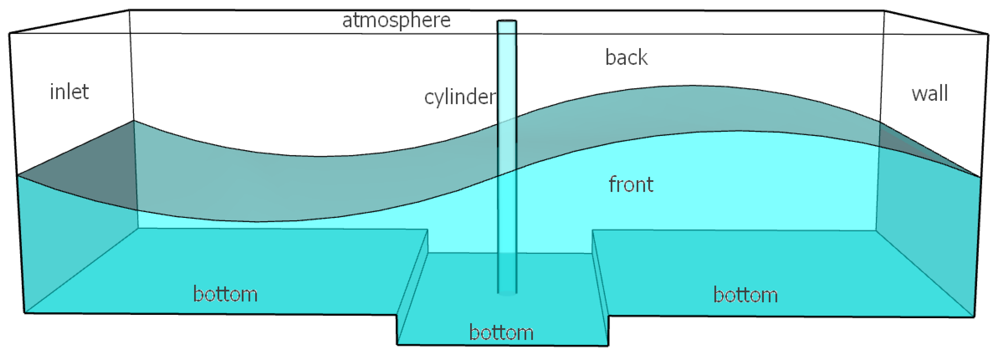
The main computational domain of this study is a three-dimensional wave flume. As sketched in Figure 1, a slot is specified on the flume bottom in the middle of the flume, to be filled with viscous fluid mud. In addition, a vertical cylinder is fixed at the center of the flume. Of course, depending on the problem to be simulated, the exact configuration of the numerical wave flume varies. The no slip condition is imposed on all solid boundaries: “wall”, “bottom”, “front”, “back”, and “cylinder”, as labeled in Figure 1; an incident solitary wave is specified on the “inlet” boundary; the “atmosphere” boundary is open to the atmosphere. Since the right wall of the flume is a solid boundary, wave reflection occurs after the incident wave reaches the right wall. Nonetheless, we analyze and present only the results before the arrival of the reflected waves. Therefore, wave reflection from the right wall is irrelevant in this study.
3. Validation Tests
OpenFOAM in combination with the olaFlow module has been widely applied to study free surface flows (see, e.g., the references provided by Higuera [42]), including the generation and propagation of solitary waves. However, to the best of our knowledge, it has not been applied to investigate wave–structure interaction over a muddy seabed. Hence, we find it necessary to perform and present validation tests relevant to the problem of interest—solitary wave interaction with a vertical cylinder over a viscous mud bed. Unfortunately, no experimental measurements resembling this configuration are available for a direct validation test. As second-best options, we select two validation tests, each resembling part of the wave–cylinder–mud problem. The two tests are: a solitary wave propagating over a viscous mud bed, and a solitary wave passing a vertical cylinder over a rigid bottom.
3.1. Solitary Wave Propagating over a Viscous Mud Bed
This section presents the validation test for a solitary wave propagating over a viscous mud bed, based on the Park et al. [27] laboratory experiment, which was conducted in a physical wave flume of length of 32 m, width m, and depth m. A piston-type wavemaker was installed on the left side of the flume. A slot of length m, width m, and height m was placed at a distance of m away from the left side of the flume. To mimic a muddy seabed, the slot was filled with a highly viscous Newtonian silicone fluid. The silicone fluid has a kinematic viscosity of 5.24 × 10⁻³ m2s−1 and a density of 1050 kg/m3. It is transparent, allowing for optical measurements of the flow. Outside of the mud slot, the flume was filled with water to a depth of m. A solitary wave with a wave height of m and an effective wavelength of m was generated by the wavemaker as the incident wave. According to Park et al. [27], based on the Reynolds number similarity, this configuration approximately translates to a prototype water depth of 10 m over a viscous mud with a kinematic viscosity of 5.36 m2s−1. In comparison, Gade [23] estimated the viscosity of the top-layer sediments in the Mississippi River Delta, USA to be between 0.1 m2s−1 and 1 m2s−1.
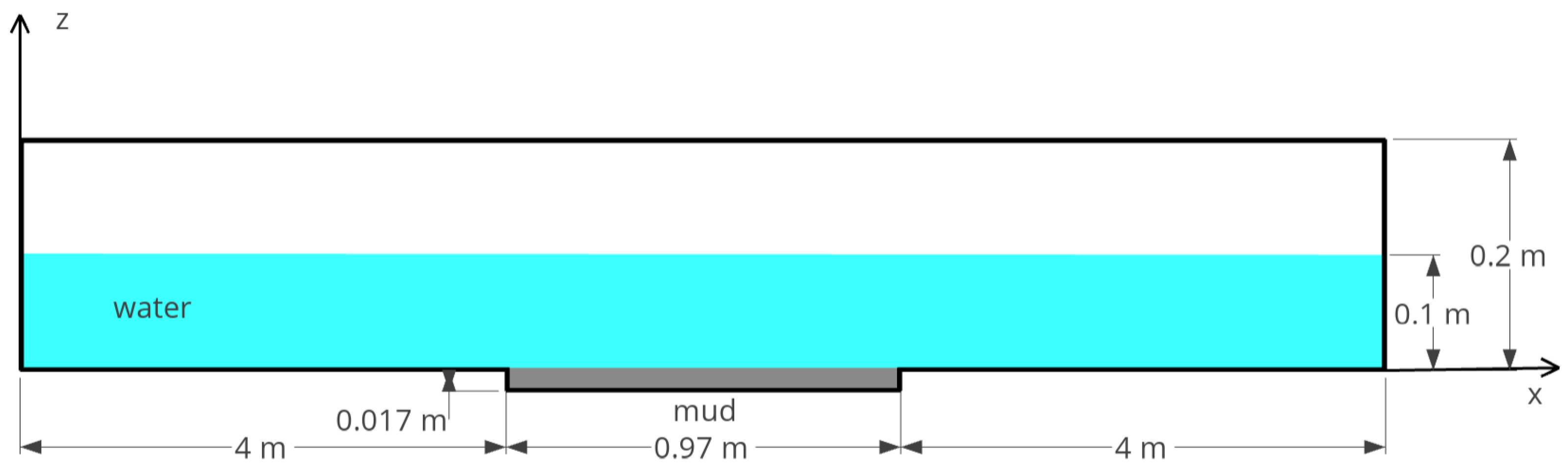
In our numerical simulations, the kinematic viscosity of water was set to be 10−6 m2s−1, and the density of water was set to be 1000 kg/m3. To increase computational efficiency, a shorter wave flume was used. As sketched in Figure 2, the numerical wave flume is 8.97 m long. The origin of the coordinate system is defined at the bottom left of the numerical wave flume; i.e., x = 0 m is defined at the left side of the flume, and z = 0 m is defined at the bottom of the left side of the flume.
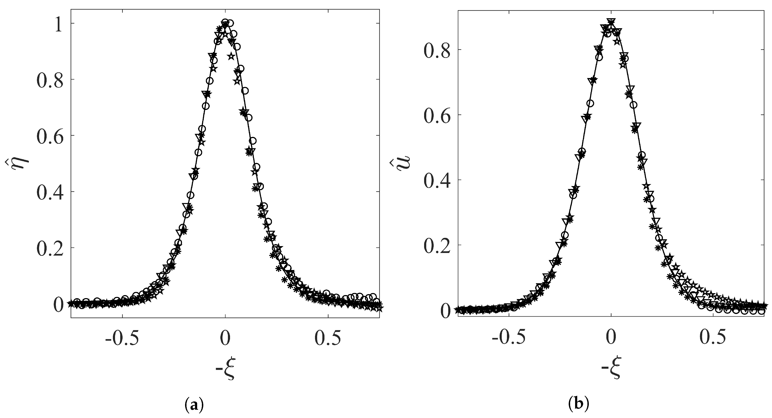
Park et al. [27] measured the water surface displacement, the water flow velocities, the mud surface displacement, and the mud flow velocities. In Figure 3, we compare the numerical results at m for the water surface and the horizontal water flow velocity (at m) with experimental measurements. Numerical results based on three different mesh sizes are shown: coarse mesh ( cm, cm), medium mesh ( cm, cm), and fine mesh ( cm, cm). The Grimshaw [3] solitary wave analytical solutions are also plotted. The same symbols and nondimensionalization factors as in Park et al. [27] are used. Thus, for brevity they need not be reiterated here. It can be seen that the results agree well with each other. The coarse-mesh results slightly underestimate the peak values, whereas the medium-mesh results are nearly identical to the fine-mesh results, indicating that the medium mesh is sufficient for simulating the water wave in this problem.
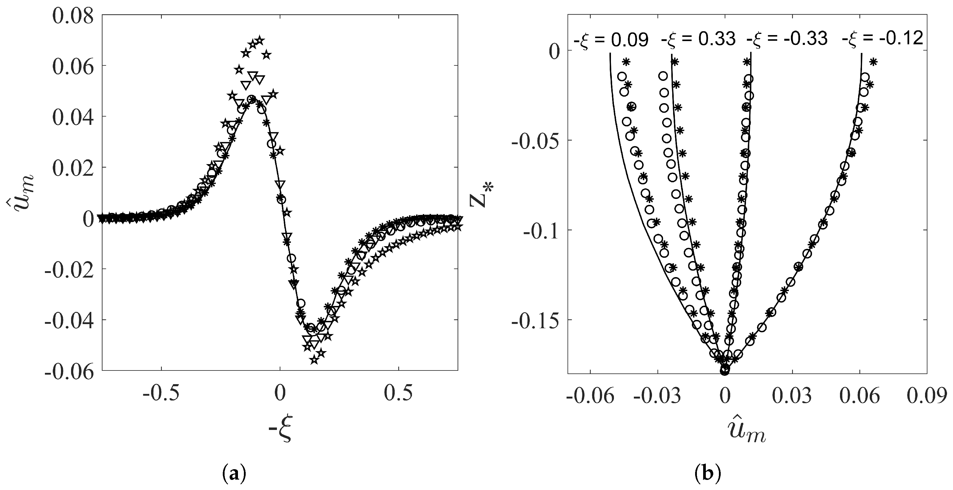
In Figure 4, we compare the numerical results at m for the horizontal mud flow velocity (at m), and the mud flow velocity profiles with experimental measurements. The analytical solutions from Liu and Chan [26] are also plotted. Again, the same symbols and nondimensionalization factors as in Park et al. [27] are used, which need not be reiterated here. In Figure 4a, numerical results based on three different mesh sizes are shown for the horizontal mud flow velocity. Although the medium mesh is sufficient for simulating the water wave, to accurately simulate the mud flow is more demanding—Figure 4a shows that the fine mesh is needed for the numerical results to agree with experimental measurements. Therefore, in Figure 4b, only the fine-mesh numerical results are shown.
Overall, good agreement between the fine-mesh numerical results and the experimental measurements is achieved. Therefore, we have validated the capability of the numerical model to simulate a solitary wave propagating over a viscous mud bed.
3.2. Solitary Wave Passing a Vertical Cylinder over a Rigid Bottom
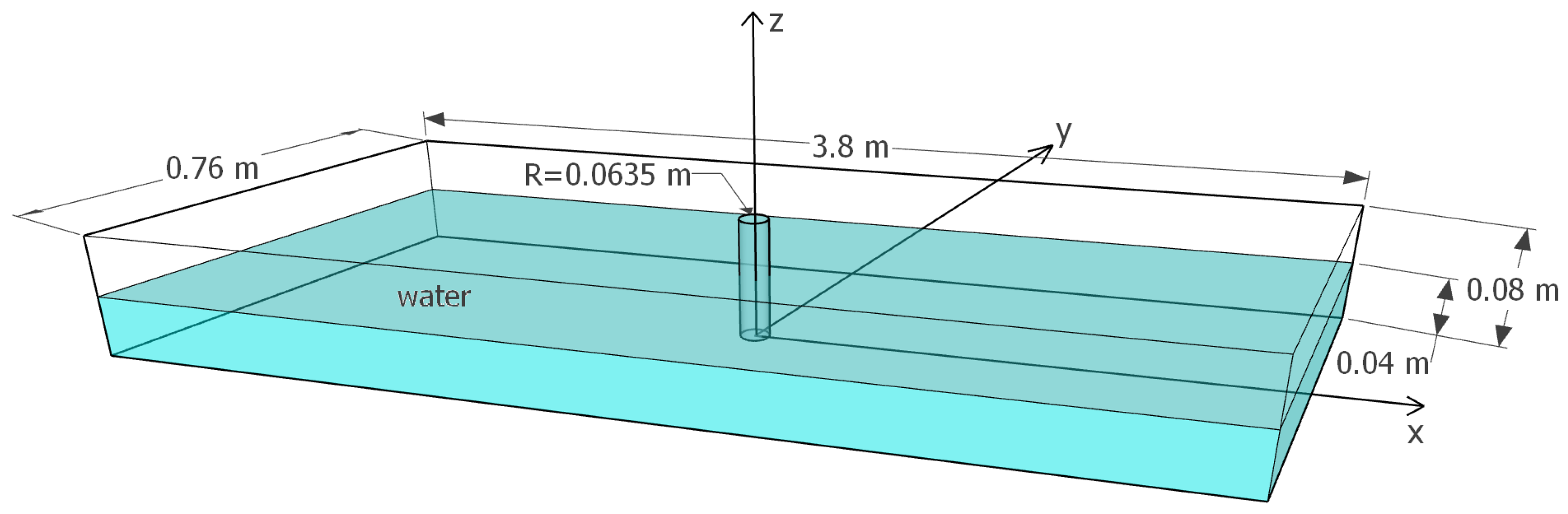
This section presents the validation test for a solitary wave passing a fixed vertical cylinder over a rigid bottom, based on the Yates and Wang [6] laboratory experiment, which was conducted in a physical wave flume of length m, width m, and height m. A piston-type wavemaker was installed on the left side of the flume. Along the center line and in the middle of the flume, a vertical cylinder of radius m and height m was installed. The still water depth was m, and the incident wave height of the solitary wave was m. According to Yates and Wang [6], this configuration falls in the large-body and shallow-water regime. The diffraction parameter is
in which D is the cylinder diameter, and l is the effective wavelength of a solitary wave, Equation (3). Based on the criterion derived by Isaacson [4], solitary wave diffraction by the cylinder is important in this experiment. For a solitary wave, Yates and Wang [6] calculated the Keulegan–Carpenter number to be
in which H is the incident wave height and h is the still water depth as defined in (1). For , drag forces can be neglected in comparison to inertia forces (see, e.g., Sarpkaya and Isaacson [45] and Yates and Wang [6]).
The three-dimensional numerical wave flume used for this validation test is sketched in Figure 5. The origin of the coordinate system is defined at the center of the base of the cylinder. x points in the streamwise direction, y points in the lateral direction, and z points in the vertical direction. To increase computational efficiency, a shorter numerical wave flume of length m was used.
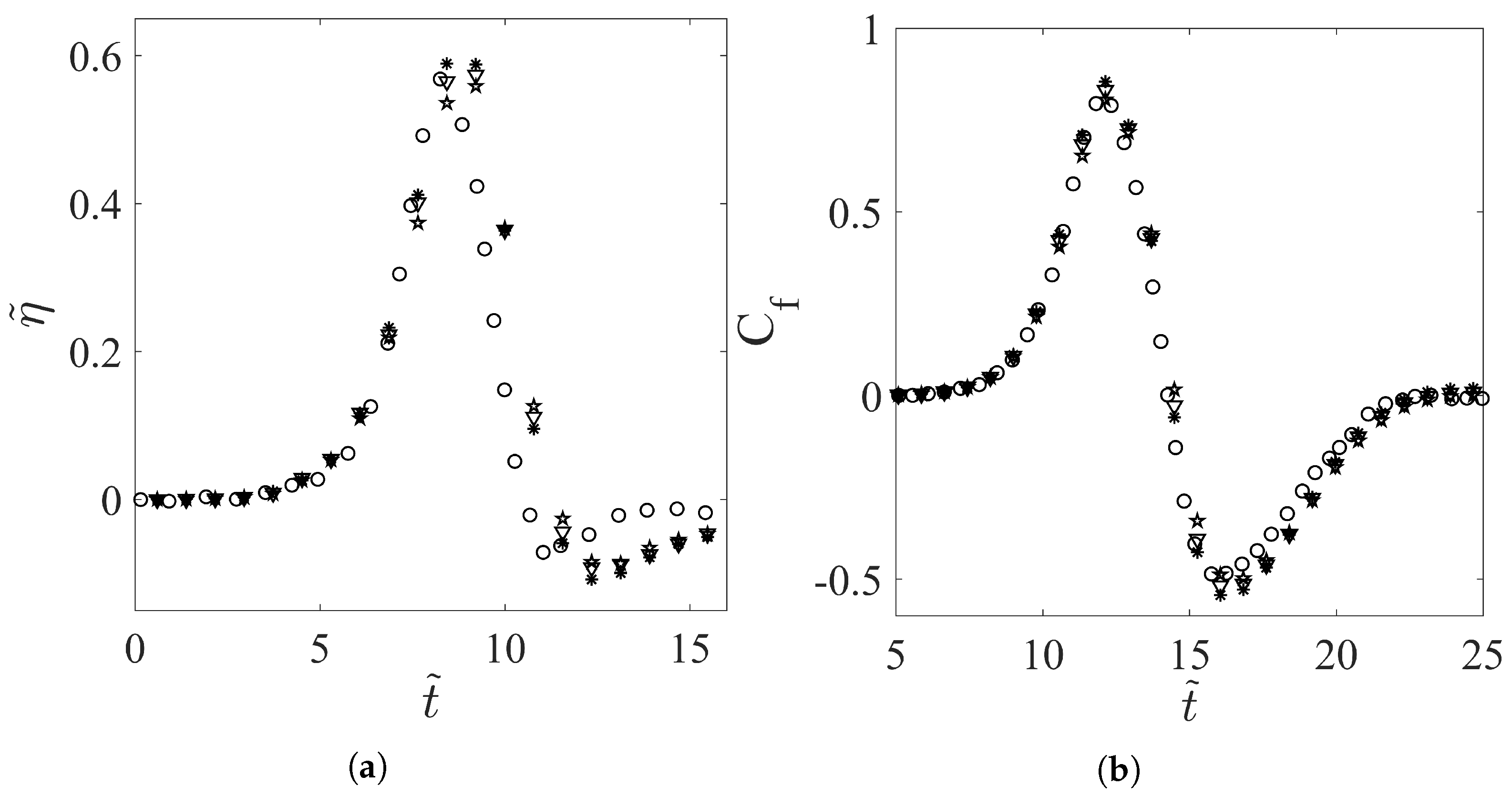
Yates and Wang [6] measured the water surface displacement and the horizontal wave force exerted on the cylinder. The numerical results are compared with experimental measurements for the water surface displacement at m in Figure 6a, and for the horizontal wave force exerted on the cylinder in Figure 6b. The same symbols and nondimensionalization factors as in Yates and Wang [6] are used. Hence, for brevity they need not be reiterated here. Numerical results based on three different mesh sizes are shown: coarse mesh (smallest cell size: cm, cm, cm), medium mesh (smallest cell size: cm, cm, cm), and fine mesh (smallest cell size: cm, cm, cm). For these three mesh sizes, the numerical results are not very sensitive to the mesh sizing, as can be seen in Figure 6.
The water surface results, i.e., Figure 6a, shows a slight difference in the wave shape between the numerical results and the experimental measurements. This is likely due to the less-than-ideal solitary wave generation in the laboratory, since this deviation from experimental measurements also shows in the numerical simulation of this problem performed by Wang et al. [5]. Aside from the slight shape difference, the overall agreement between the numerical results and the experimental measurements is good. Therefore, we have validated the capability of the numerical model to simulate a solitary wave passing a fixed vertical cylinder over a rigid bottom.
4. Setup of Numerical Investigation
Having validated the numerical model for simulating wave–mud interaction and wave–cylinder interaction, we shall begin the numerical investigation on the wave–mud–cylinder interaction. This section is dedicated to describing the numerical configuration. The results will be presented in the next section.
4.1. Numerical Experiments
Adopting the concept of control variables, we devised four numerical experiments. The configurations of these four numerical experiments are summarized in Table 1. Comparing the results from these four numerical experiments shall reveal the influences of the cylinder, of the bottom slot, and of the fill material placed in the bottom slot. The same incident wave, a solitary wave with , was used in all four numerical experiments.
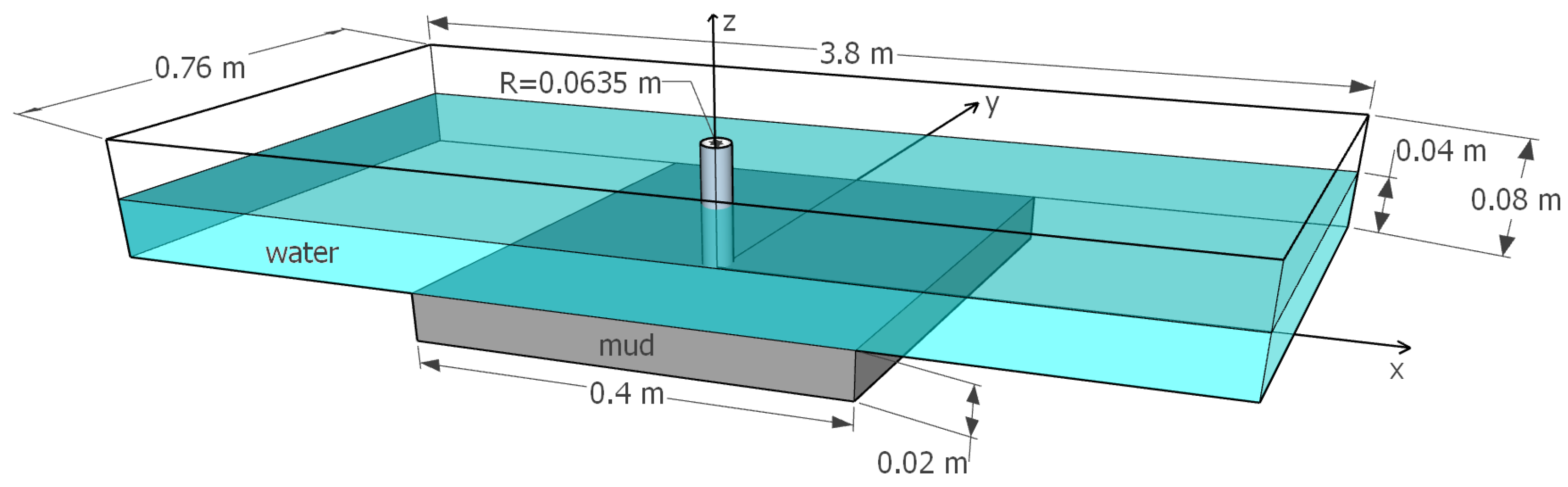
As an example, the numerical wave flume used for test1 is sketched in Figure 7. The origin of the coordinate system is defined at the center of the cylinder and on the initial water–mud interface. Therefore, in still water, water occupies , and the viscous fluid mud occupies . To ensure that the numerical simulations are within the validated range of applicability, scaling and parameter choice in the present investigation are based purely on existing laboratory experiments.
As in the validation test based on the Yates and Wang [6] experiments, the still water depth is m, the incident solitary wave has a wave height of m, and the effective wavelength is m. Since these scales are the same as those in Yates and Wang [6], the wave–cylinder interaction falls in the large-body and shallow-water regime. The diffraction parameter is , Equation (4)—wave diffraction by the cylinder is significant; the Keulegan–Carpenter number is , Equation (5)—drag forces are negligible in comparison to inertia forces.
As indicated in Figure 7, a bottom slot of length m, width m, and depth m is installed in the middle of the flume. The vertical cylinder extends all the way to the bottom of the slot; i.e., m. The slot is filled with the highly viscous silicone fluid used by Park et al. [27]. Its kinematic viscosity is 5.24 × 10⁻³ m2s−1, and its density is 1050 kg/m3. The kinematic viscosity of water is set to be 10−6 m2s−1, and the density of water is set to be 1000 kg/m3. Since the water depth and the mud slot depth are both different from the Park et al. [27] experiment, the prototype scales are also different. Based on the Reynolds number similarity proposed by Park et al. [27], our numerical configuration approximately translates to a prototype water depth of 10 m over a viscous mud with a kinematic viscosity of 20.71 m2s−1, about four times more viscous than the prototype viscosity of the Park et al. [27] experiment.
4.2. Mesh Configuration
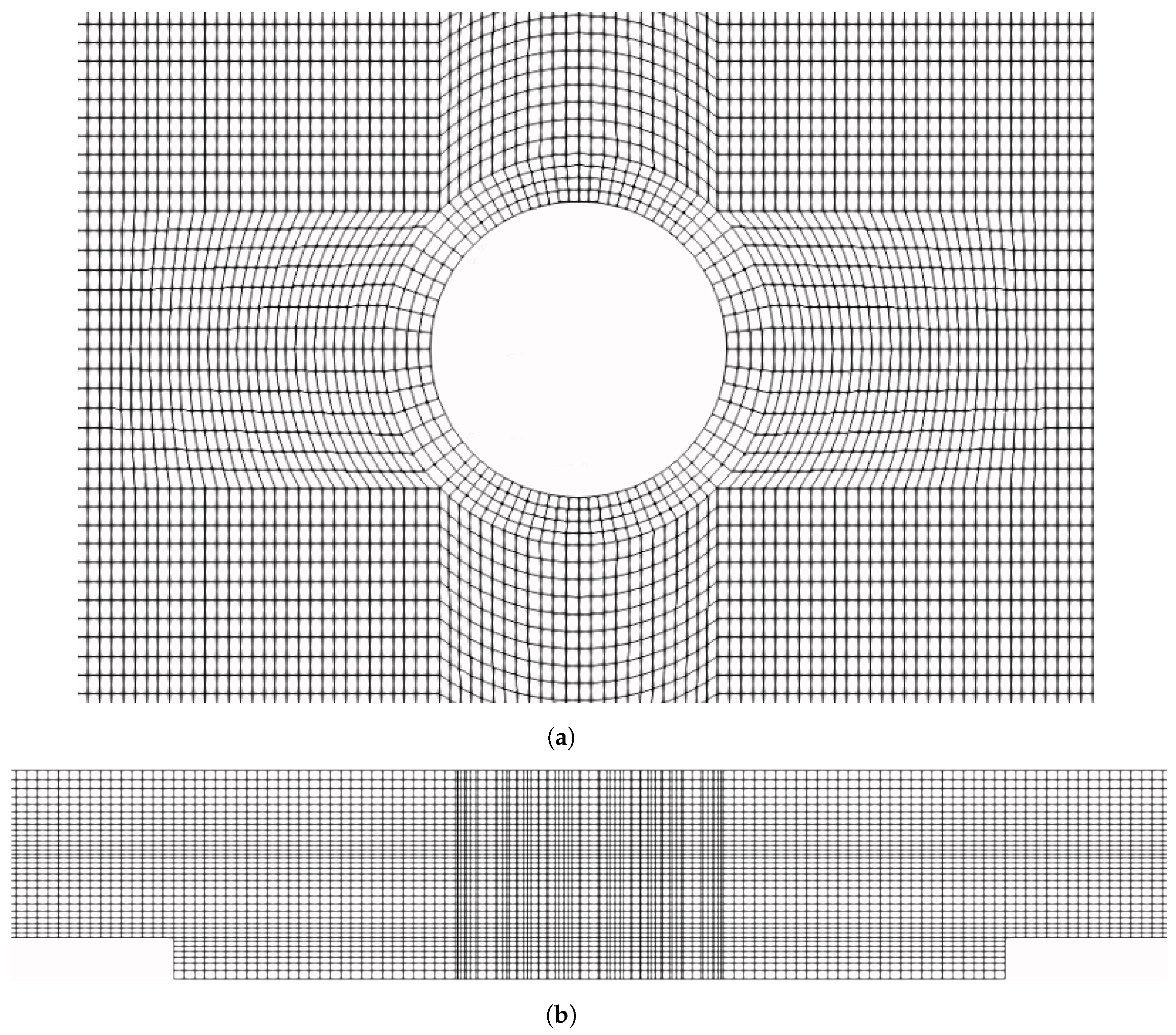
As sketched in Figure 8, a structured yet nonuniform mesh is used. Since our main interests are the fluid interfaces and flows near the slot and the cylinder, a graded mesh is utilized. Mesh spacing in the x-direction is coarser near the two ends of the flume and gets finer near the slot; mesh spacing in the z-direction is finer near the air–water interface and the water–mud interface; mesh spacing in the y-direction is uniform. As can be seen in Figure 8a, the mesh is curvilinear near the cylinder; elsewhere, the mesh is rectilinear.
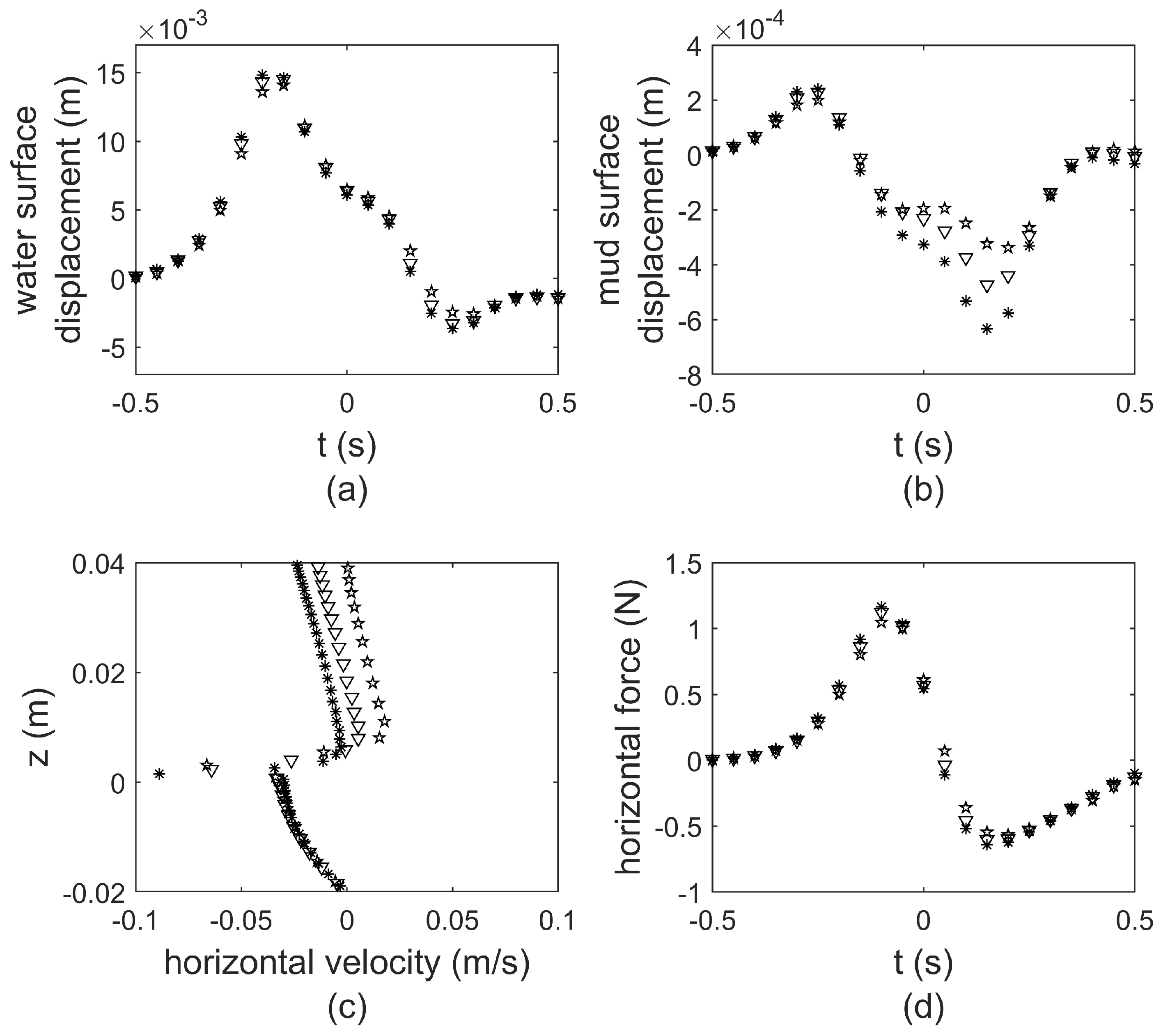
Mesh convergence tests for test1 were conducted based on this mesh configuration. In the coarse mesh, the smallest cell size is cm. In the medium mesh, the smallest cell size is cm. In the fine mesh, the smallest cell size is cm. Comparisons of the numerical results for the water surface displacement at m, the mud surface displacement at m, the velocity profile at m, and the horizontal force exerted on the cylinder are shown in Figure 9. While the results based on differently sized meshes agree well with each other for the water surface displacement and the horizontal force, discrepancies are noticeable for the mud surface displacement and the velocity profile. We note that the mud surface displacement is one order of magnitude smaller than the water surface displacement. In addition, the mud surface displacement is smaller than the vertical mesh spacing, and the VOF method is not designed to precisely track the interfaces. Despite the discrepancies, the trends and characteristics of the results agree with each other regardless of the mesh size.
Numerical experiments with an event duration of 5 s were simulated on the Intel i7-9800X CPU ( GHz ). The coarse-mesh computation time is approximately 10 h, the medium-mesh computation time is approximately 7 days, and the fine-mesh computation time is approximately 54 days. As this study is a preliminary investigation focusing more on the qualitative understanding, rather than precise quantitative measurements, of an underexplored problem, the coarse mesh was adopted due to its feasibility and computational efficiency. More details on the mesh configuration based on the coarse mesh are tabulated in Table 2 for the four numerical experiments to be investigated.
5. Results
Having described the mesh configuration, we now present and discuss the numerical results based on the coarse mesh for the four numerical experiments listed in Table 1. The incident solitary wave travels from negative x towards positive x. s is defined as the instant when the freestream (i.e., away from the cylinder) wave crest passes . Therefore, the wave is upstream of the cylinder for s, and downstream of the cylinder for s.
5.1. Water Surface and Mud Surface
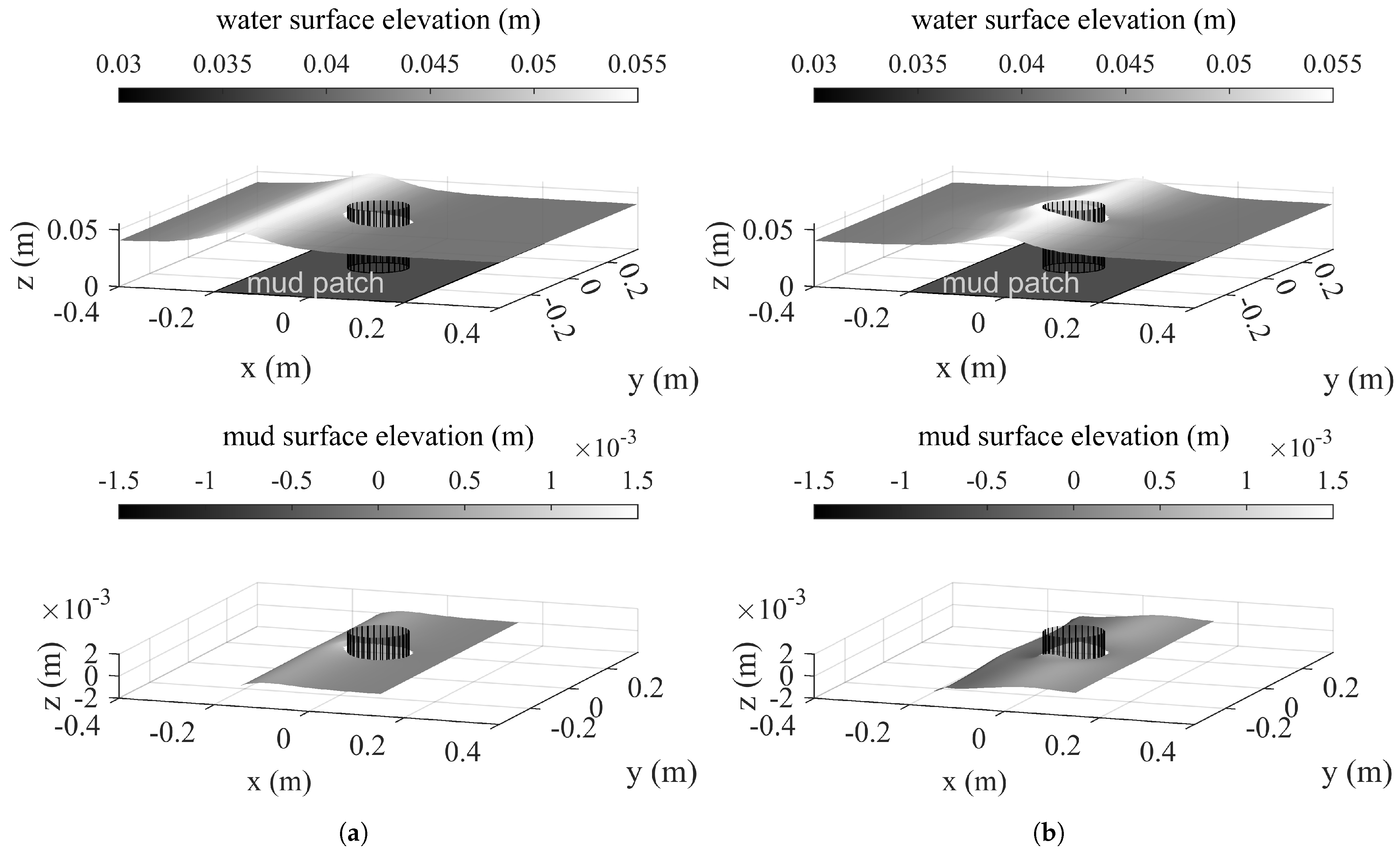
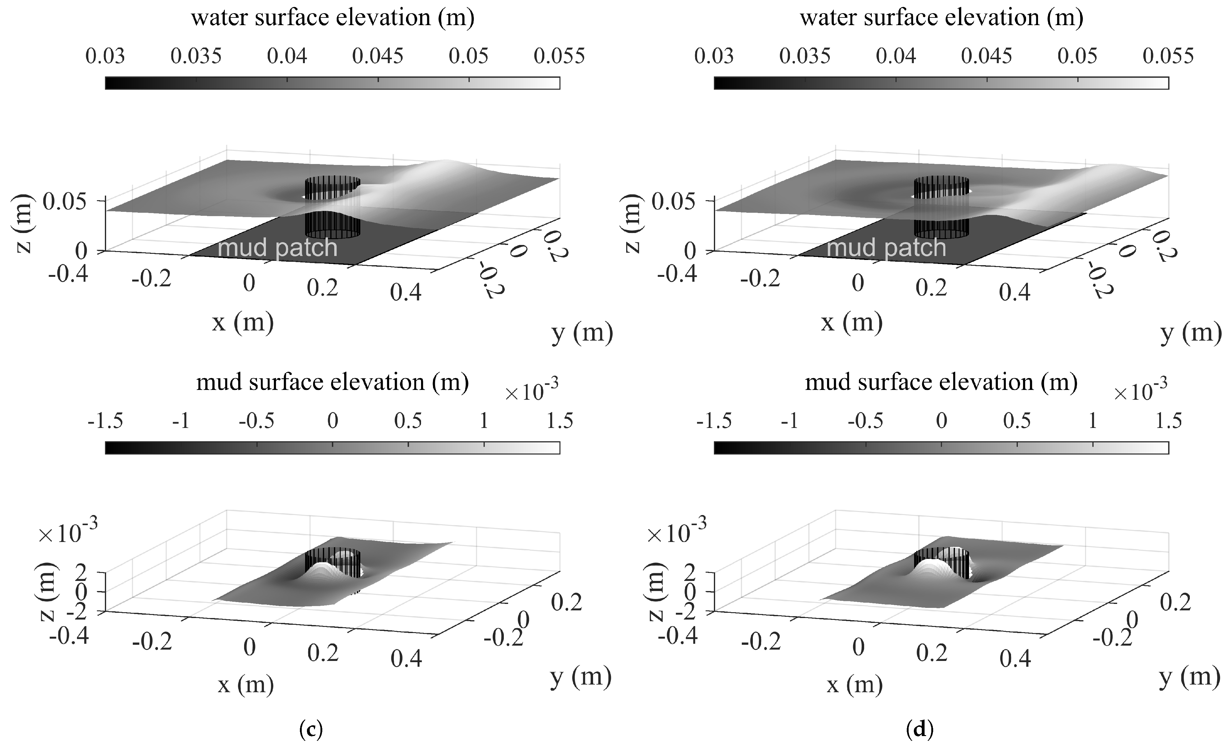
Snapshots of the water surface displacement and the mud surface displacement are shown in Figure 10 from s to s. In Figure 10a at s, the wave crest approaches the cylinder. Both the water surface and the mud surface rise upstream of the cylinder. In Figure 10b at s, the wave crest reaches the lateral axis of the cylinder ( m). Water surface upstream of the cylinder and on the lateral sides of the cylinder rises. The mud surface rises on the lateral sides of the cylinder. However, depressions occur on the mud surface upstream of the cylinder. In Figure 10c at s, the wave is just downstream of the cylinder. Wave runup on the cylinder can be observed on the downstream side. Due to wave scattering, an area of water surface depressions shows on the upstream and lateral sides of the cylinder. The mud surface also shows a depression upstream of the cylinder. However, differently from the water surface, on the lateral sides, the mud surface rises; a slight mud surface depression also shows immediately downstream of the cylinder. In Figure 10d at s, the wave has just left the cylinder. The water surface depression due to wave scattering continues radiating outwards from the cylinder. The mud surface depression upstream of the cylinder remains, the mud surface elevation on the lateral sides of the cylinder rises near to a maximum, and the mud surface depression downstream of the cylinder also grows near to a maximum extent.
From all panels of Figure 10, it can be seen that the mud surface displacement is one order of magnitude smaller than the water surface displacement; i.e., mm vs. cm. The water wave height is slightly reduced by the mud bed as expected per the derivation by Liu and Chan [26]. Nonetheless, the overall solitary wave scattering pattern due to a vertical cylinder remains similar to that predicted by Wang et al. [5]. Although the mud surface displacement is induced by the water waves, it deforms differently from the water surface displacement—on the upstream side of the cylinder, the mud surface first rises, and then depresses; on the lateral sides of the cylinder, the mud surface rises; on the downstream side of the cylinder, the surface depresses. These seabed deformation characteristics differ significantly from typical solitary-like wave scour on a sandy seabed around a cylinder, which tend to show a scour hole around the cylinder, and sediment deposits some distance downstream of the cylinder (see e.g., Larsen et al. [12], Li et al. [16]). Albeit the present study is a preliminary investigation assuming a highly idealized fluid mud model (i.e., a highly viscous Newtonian fluid), it nonetheless reveals the possibility of achieving a different scour pattern in the event of a muddy seabed, as opposed to the commonly assumed sandy seabed. As the scour problem is important in both foundation design and sediment transport, further investigations assuming a more realistic mud model may be needed.
5.2. Velocity Field
Just like the water surface, the freestream (i.e., away from the mud bed) water flow velocity is only slightly affected by the mud bed. Since the freestream water flow velocity is similar to that in existing studies on a solitary wave passing a vertical cylinder over a rigid bottom (e.g., Isaacson [4], Wang et al. [5]), our focus is on the water flow velocity near the mud bed and the mud flow velocity, which are understudied phenomena that warrant further discussions.
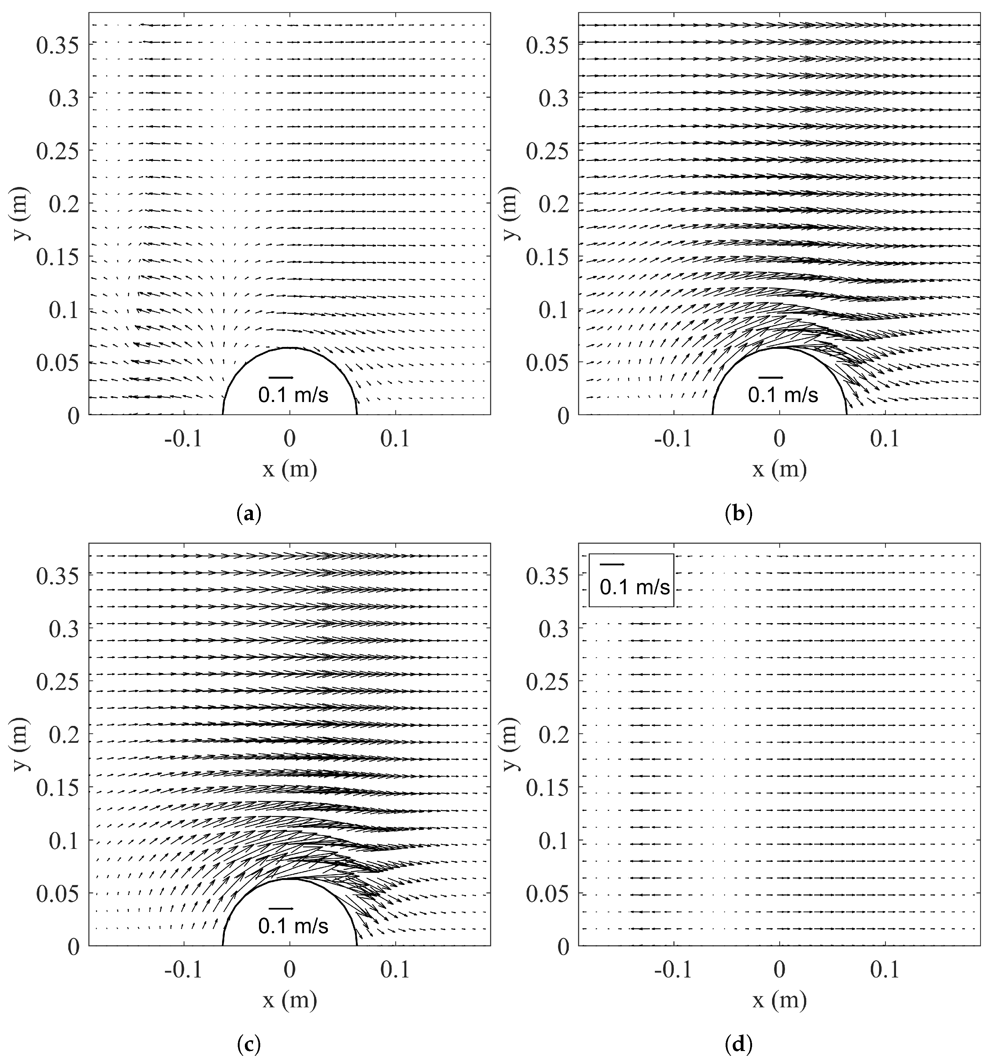
Snapshots of the horizontal water flow field at m (near the water–mud interface or the water–solid bottom boundary) and s (when the wave crest reaches m) are shown in Figure 11 for the four numerical experiments listed in Table 1. In Figure 11b,c, where no mud is present, a typical flow-around-a-cylinder pattern shows, with the horizontal velocities mostly pointing towards the positive direction. However, in Figure 11a,d, where a mud bed is present, flow reversal can be clearly observed: the horizontal velocities are zero near m, positive for m, and negative for m. In addition, the flow speeds in Figure 11a,d are noticeably smaller than those in Figure 11b,c—namely, the water–mud interface slows down the flow more than the water–solid interface. On the other hand, due to an increase in the effective local water depth in test3, to satisfy mass conservation the flow speeds in Figure 11b appear slower than those in Figure 11c. By comparing Figure 11a with Figure 11d, it can also be seen that the existence of the cylinder increases the reverse flow speeds immediately upstream of the cylinder.
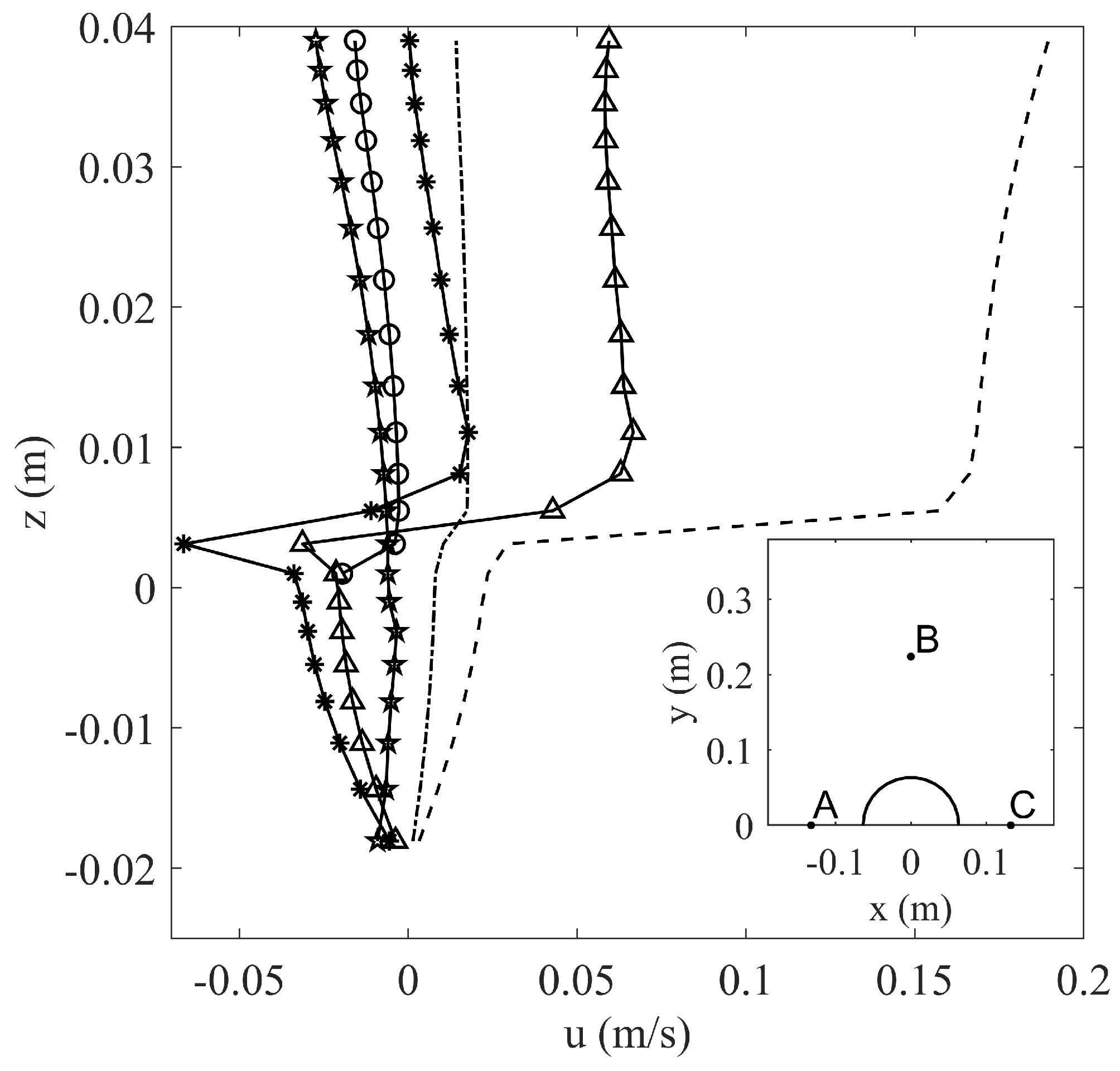
To show the vertical distributions of the horizontal velocities, the velocity profiles at three representative locations are examined—the upstream location m, the freestream location m, and the downstream location m, as sketched in the bottom right of Figure 12. Velocity profiles from the four numerical experiments listed in Table 1 are plotted in Figure 12 at s.
At the upstream location A, both the test1 results and the test4 results show a reversal of water flow—the horizontal velocity changes sign near m in test1, and the horizontal velocity changes sign near m in test4. This difference in the elevation of water flow reversal is most likely due to the damming effects of the cylinder—the only configuration difference between test1 and test4. In addition, the mud flow velocity also points in the negative direction, and its overall magnitude is smaller than the water flow.
In the results for test2 and test3, where no mud is present, water flow reversal is not evident under the present mesh resolution, indicating that the presence of a mud bed enlarges the region in which flow reversal may occur.
At the freestream location m and the downstream location m, flow velocities for test1 are all positive. It can be seen that water flow is slowed down near the water–mud interface, and that the mud flow is noticeably slower than the water flow.
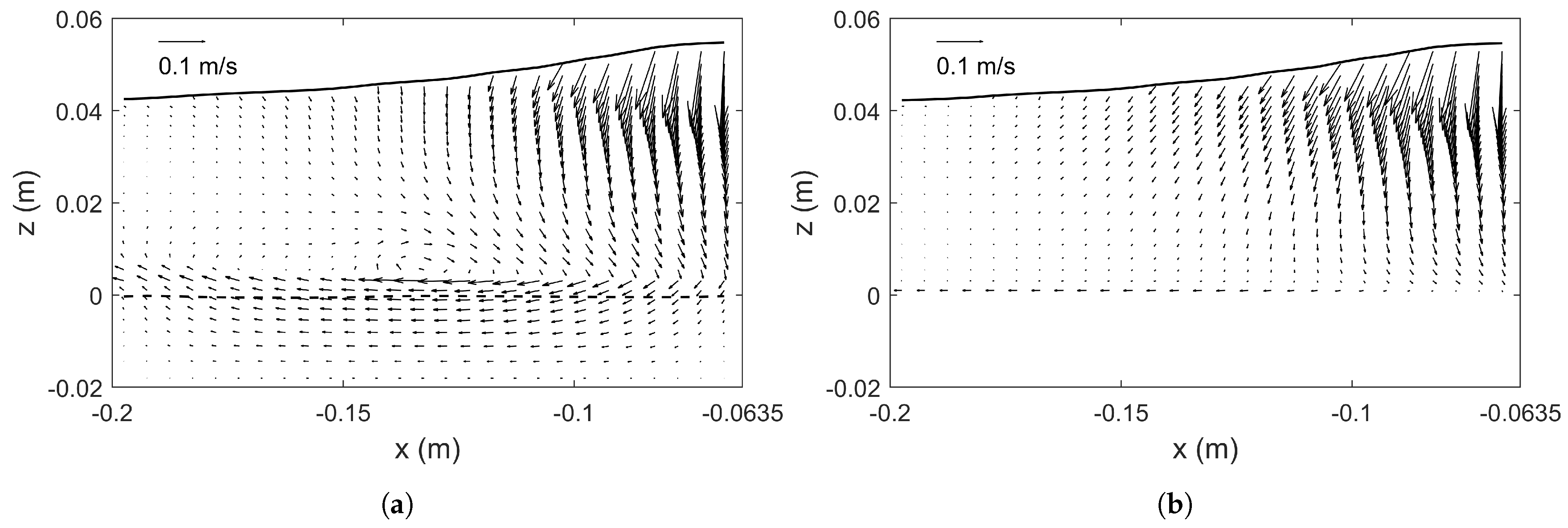
In test1, due to the presence of both a vertical cylinder and a viscous mud bed, a clockwise vortex on the -plane forms immediately upstream of the cylinder when the local water surface starts to fall. This phenomenon resembles the horseshoe vortex commonly observed in the scour problem. A snapshot at s is shown in Figure 13a for test1. As shown in Figure 13b for test3, this phenomenon is not evident in the absence of a mud bed.
After inspecting the velocity results in Figure 11, Figure 12 and Figure 13, it is found that the mud bed not only slows down the water flow near the water–mud interface, but also appears to facilitate water flow reversal. Hence, in the next section we shall examine the flow reversal phenomenon further.
5.3. Flow Reversal
Water flow reversal near the water–mud interface is observed in the numerical results. Liu et al. [38] pointed out that flow reversal tends to occur within boundary layers. Therefore, the study on water flow reversal is closely linked to the study of wave-induced boundary layer flow, on which various studies exist; e.g., Keulegan [36], Liu and Orfila [37], Liu et al. [38] examined the water boundary layer of a solitary wave over a rigid bottom, and Dalrymple and Liu [24], Jiang and Zhao [25], Liu and Chan [26], Park et al. [27] examined the mud boundary layer induced by a solitary wave traveling over a mud bed.
Existing studies did not consider the boundary layer induced by a solitary wave passing a vertical cylinder, nor was particular attention paid to the water flow reversal phenomenon for waves traveling over a muddy seabed. Hence, this section shall further discuss this phenomenon based on the newly obtained numerical results. We stress that this study is intended as a preliminary investigation of an underexplored problem, thus an elaborate boundary layer flow analysis is beyond the scope of this study.
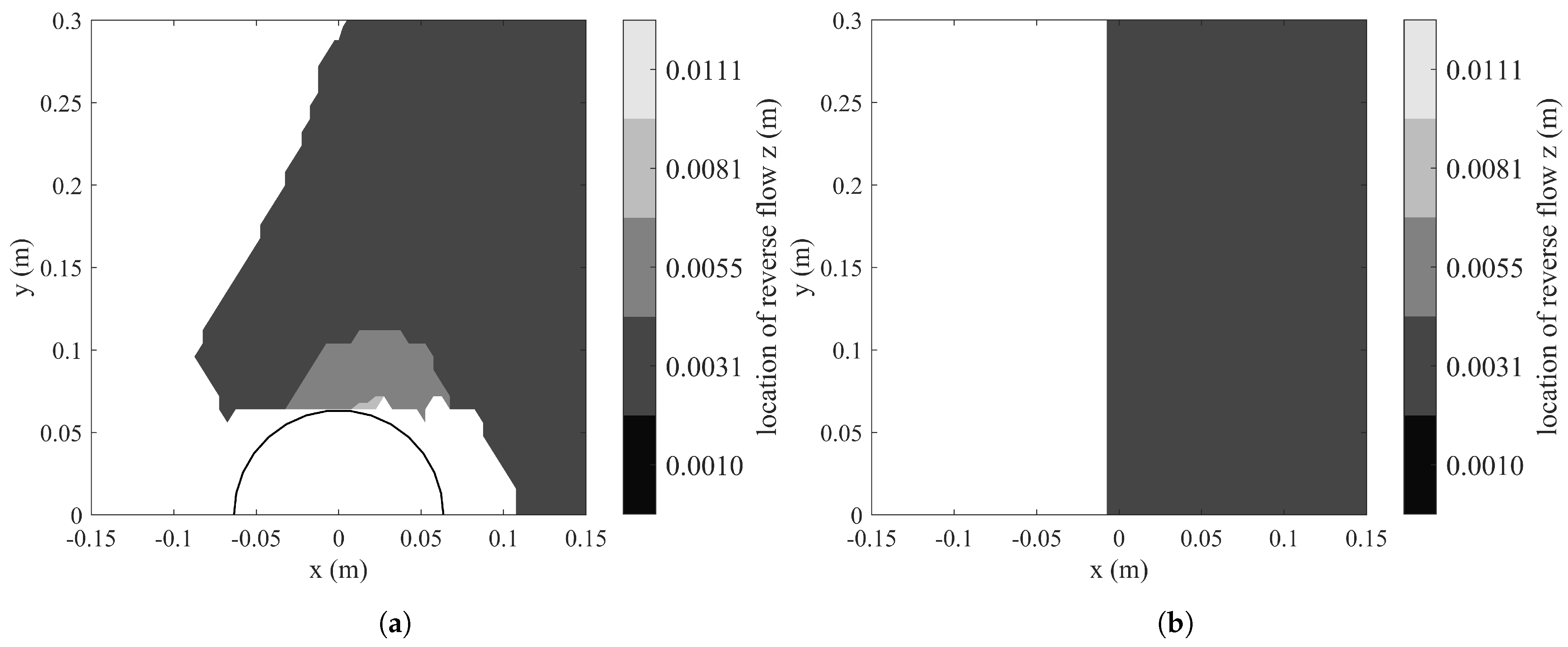
To better visualize the location where flow reversal occurs, we define the vertical location where flow reversal occurs as the vertical location where the horizontal velocity in the x-direction changes sign; a linear velocity distribution between two vertically adjacent numerical cells is assumed. An example comparing the test1 results and the test4 results at s is shown in Figure 14. Because of the existence of a mud bed, water flow reversal is facilitated and captured in both cases using the present mesh resolution. The effects due to the cylinder are evident—it allows water flow reversal to occur further upstream near the cylinder and increases the vertical location of occurrence on the lateral sides of the cylinder. However, water flow reversal does not occur immediately downstream of the cylinder.
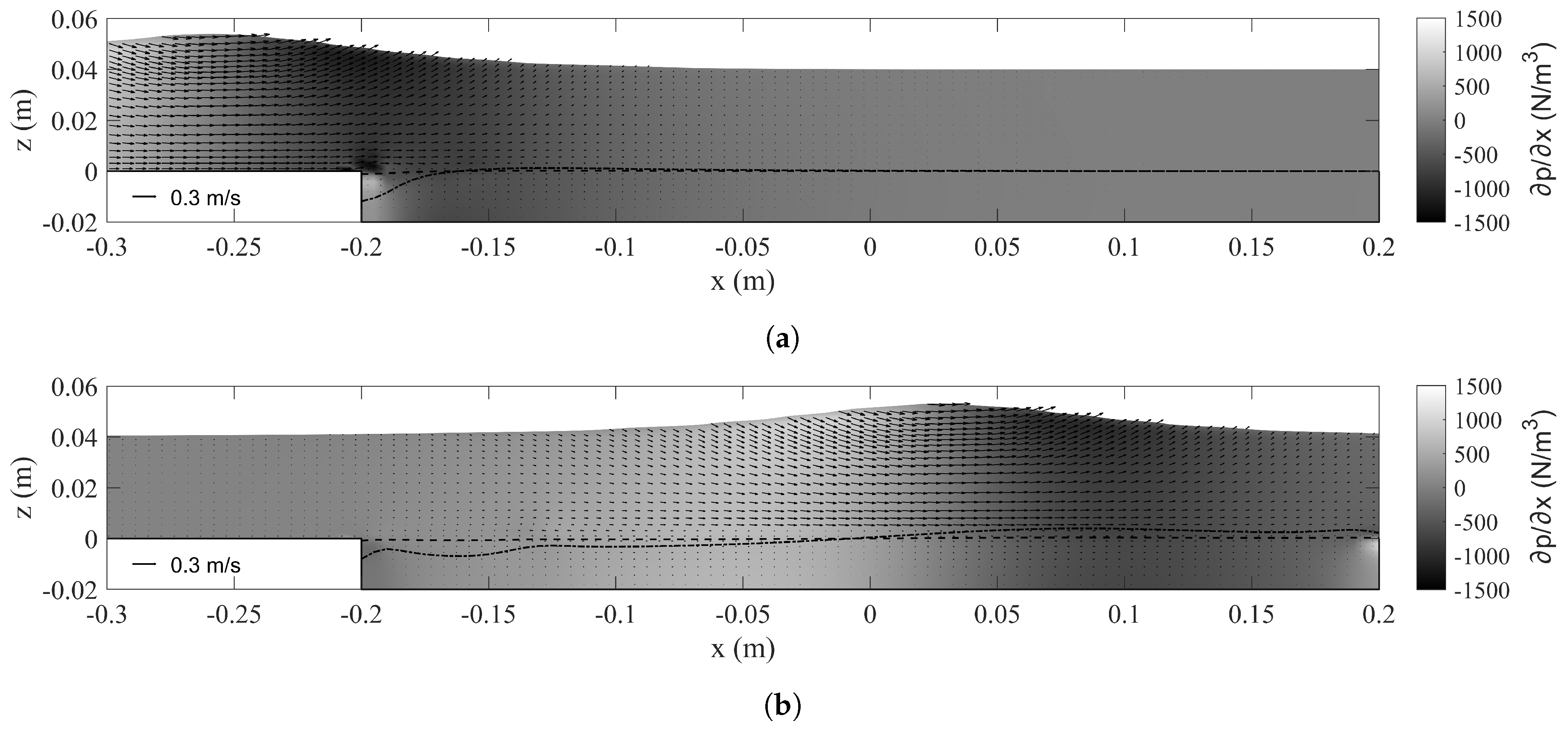
Next, we examine the simpler case test4 more closely. As suggested by Liu and Chan [26], in wave–mud interaction, a pressure gradient can be used to explain the behaviors of the mud flow and the water flow near the water–mud interface. Therefore, we shall utilize the numerical results for test4 to examine the relations between the water surface, the pressure gradient, and water flow reversal. A two-point central difference is adopted to estimate the horizontal pressure gradient . Snapshots at s and s are provided in Figure 15.
As can be seen in Figure 15, the pressure gradient is negative ahead of the wave crest and is positive behind the wave crest. Flow reversal occurs in the presence of a positive pressure gradient, which is referred to as the wave deceleration phase by Liu et al. [38]. It can also be seen that regardless of whether flow reversal occurs or not, water flow velocities near the water–mud interface are noticeably smaller than those in the freestream. The near-interface region (approximately mm), in which water flow slows down, is significantly larger than the solitary wave boundary layer thickness of mm predicted by Liu and Chan [26]. Hence, the numerical results seem to imply that the mud bed increases the thickness of the water boundary layer induced by a solitary wave propagating over a viscous mud bed; in Liu and Chan [26], the boundary layer thickness is assumed to be the same regardless of whether the bottom is rigid or a viscous mud bed. Another possible explanation is that the water flow near the water–mud interface slows down due to the momentum transfer to the mud flow.
To summarize, the flow reversal phenomenon is further discussed in this section. Although the flow reversal under a solitary wave over a rigid bottom has been well studied by Liu and Orfila [37] and Liu et al. [38], that over a viscous mud bed has not been studied carefully. Liu and Chan [26] assumed the solitary wave boundary layer thickness on a viscous mud bed to be the same as that on a rigid bottom. However, newly obtained numerical results suggest that may be untrue—a vast difference between the mm thickness predicted by existing theory and the ∼3 mm thickness observed in the numerical results. As a preliminary investigation, the present mesh resolution in the vertical direction is at best 2 mm, which is inadequate for precisely describing boundary layer flow characteristics. Therefore, future investigations focusing more on this subject are needed.
5.4. Mud Flow
Per the expressions provided by Park et al. [27], the ratio of the mud layer thickness to the mud boundary layer thickness in the present numerical experiments is estimated to be . The ratio was in the Park et al. [27] laboratory experiments. As the ratio is smaller than one, the mud flow is purely a boundary layer flow and has an approximately parabolic profile according to Park et al. [27]. As can be seen in Figure 12, this is indeed true.
Since the mud flow in the numerical experiments is a boundary layer flow, it is primarily driven by the viscous effects and the pressure gradient. As can be seen in Figure 15, the mud flow corresponds nearly instantly to the pressure gradient—the mud moves forward in the presence of a negative pressure gradient ahead of the wave crest, decelerates quickly, and eventually moves in the opposite direction in the presence of a positive pressure gradient behind the wave crest. In addition, both the mud surface and the mud flow velocities demonstrate oscillatory characteristics. While the water surface and the freestream velocities of a solitary wave are strictly nonnegative, those of the mud oscillate between positive and negative values.
5.5. Forces and Moments
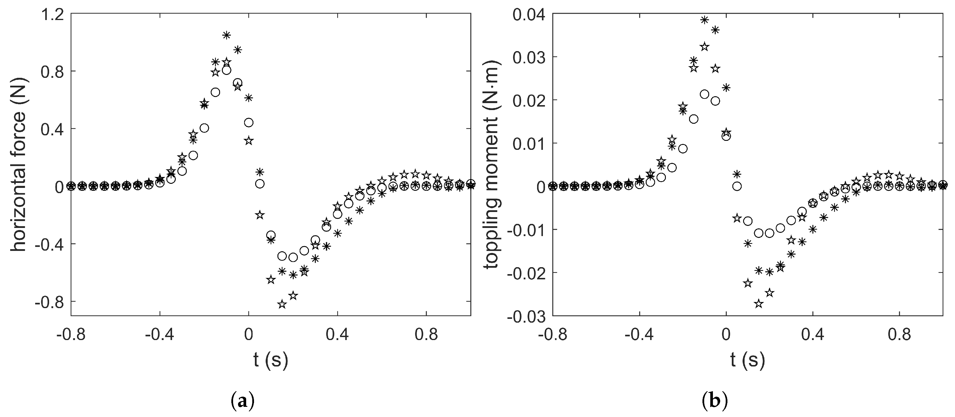
Wave forces and moments exerted on a vertical cylinder are of practical engineering value. The horizontal forces exerted on the cylinder from the three numerical experiments listed in Table 1 that have a vertical cylinder are compared in Figure 16a; the toppling moments are compared in Figure 16b. A positive force means a net force in the positive x-direction; a negative force means a net force in the negative x-direction. Mud flow induced forces are included in the force calculation whenever applicable (i.e., in test1 and test2). Toppling moments are taken at the base of the cylinder along the pitch axis; i.e., along the line for test1 and test2, and along the y-axis for test3, per the coordinate system sketched in Figure 7. A positive toppling moment means a moment that tends to topple the cylinder towards the downstream direction; a negative toppling moment means a moment that tends to topple the cylinder towards the upstream direction.
Two extreme values can be identified in all three numerical experiments in Figure 16a—a peak whose magnitude we shall refer to as the “maximum positive force” and a trough whose magnitude we shall refer to as the “maximum negative force”. In all three numerical experiments, the horizontal force exerted on the cylinder first rises to the maximum positive force, drops to the negative positive force, and then attenuates back to zero. In each of the three cases, the maximum positive force is larger than the maximum negative forces. These features are typical for a solitary wave passing a vertical cylinder, as can be seen in Yates and Wang [6] and in the validation test results (Figure 6).
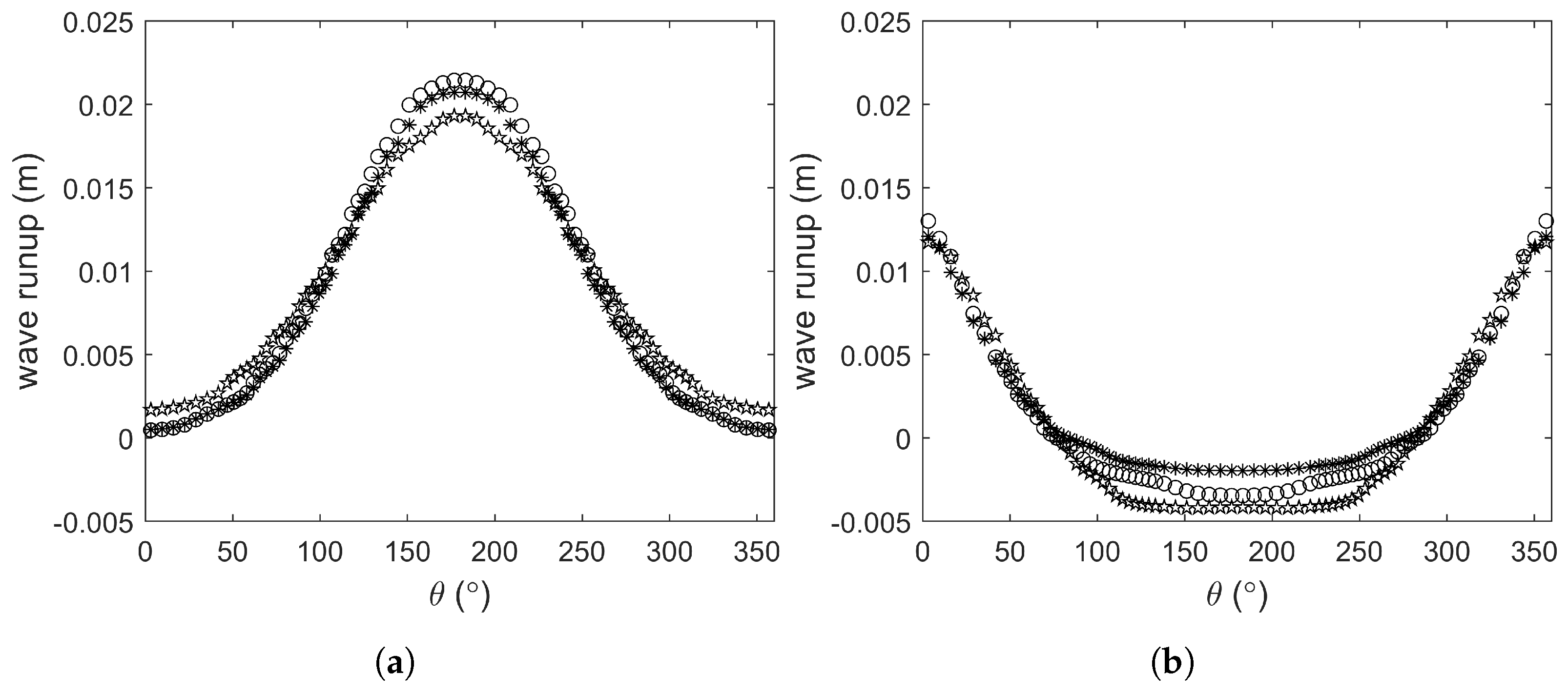
Wave runup around the cylinder changes the effective area used in the calculations of wave forces. At two instants, s, approximately when the maximum positive force occurs, and s, approximately when the maximum negative force occurs, wave runup around the cylinder is plotted in Figure 17. The polar coordinate system is used in the figure, such that points in the downstream direction and points in the upstream direction. It can be seen that the difference between the runup results is small. Therefore, the slight difference in the wave runup among the three numerical experiments does not explain the differences in the horizontal wave forces observed in Figure 16a.
The remaining factors causing the differences in the horizontal wave forces are then the existence of a bottom slot and the fill material placed in the slot. From Figure 16a, it can be seen that the existence of a bottom slot (i.e., test1 and test2) increases both the maximum positive force and the maximum negative force. If the slot is filled with viscous mud (i.e., test1), the maximum positive force becomes the largest of the three cases; if the slot is filled with water instead (i.e., test2), the maximum negative force becomes the largest of the three cases. A breakdown of the maximum forces is provided in Table 3.
Comparing the test2 results with the test3 results in Figure 16a reveals that both the maximum positive force and the maximum negative force are larger in test2, and the difference in the maximum negative force is more pronounced. The breakdown in Table 3 shows that the contribution from the above-slot region ( m) to the maximum positive force in test2 is actually smaller than that in test3. However, when the contribution from the slot region ( m) is added, the total maximum positive force in test2 becomes larger than that in test3. In contrast, the contribution from the above-slot region to the maximum negative force in test2 is already larger than that in test3. When the contribution from the slot region is added, the total maximum negative force in test2 becomes even larger.
Comparing the test2 results with the test1 results in Figure 16a reveals that changing the fill material in the slot from water to viscous mud makes the maximum positive force larger but makes the maximum negative force smaller. The breakdown in Table 3 shows that both the contribution from the above-slot region and the contribution from the slot region to the maximum positive force in test1 are larger than those in test2; similarly both the contribution from the above-slot region and the contribution from the slot region to the maximum negative force in test1 are smaller than those in test2.
Comparing the test1 results with the test3 results in Figure 16a reveals that both the maximum positive force and the maximum negative force are larger in test1, and the difference in the maximum positive force is more pronounced. The breakdown in Table 3 shows that the contribution from the above-slot region to the maximum positive force and the maximum negative force in test1 are both smaller than those in test3. However, when the contribution from the slot region is added, both the total maximum positive force and the total maximum negative force in test1 become larger than that in test3. Therefore, although a muddy seabed is capable of attenuating wave energy, the wave energy transferred to the mud may induce mud flow, which in turn may increase the total loading on a marine structure.
To summarize, comparing the test2 results with the test3 results shows that the existence of a bottom slot increases the maximum horizontal forces exerted on the cylinder; comparing the test2 results with the test1 results shows that a bottom slot filled with mud increases the maximum positive force but decreases the maximum negative force, as compared to a bottom slot filled with water; comparing the test1 results with the test3 results shows that although a viscous mud bed attenuates wave energy, it nonetheless increases the total horizontal forces exerted on the cylinder due to the wave-induced mud flow.
Lastly, we examine the toppling moments exerted on the cylinder. The time series is shown in Figure 16b and a breakdown is provided in Table 4. The overall trends of the toppling moments are similar to those of the horizontal wave forces—both the maximum positive moment and the maximum negative moment increase if a bottom slot is considered, and a bottom slot filled with viscous mud results in the largest maximum toppling moment. The discussions on the wave forces also apply to the toppling moments. In terms of the toppling moments, the differences between the results from the three numerical experiments become even more pronounced.
6. Concluding Remarks
This study constructed and validated a three-dimensional numerical wave flume to investigate solitary wave interaction with a vertical cylinder over a highly viscous Newtonian fluid mud bed. Numerical experiments were performed to investigate the water surface displacement, the mud surface displacement, the velocity field, and the forces and moments exerted on the vertical cylinder in the wave–cylinder–mud problem. The main findings include:
- The mud surface deformation is one order of magnitude smaller than the water surface deformation and their deformation patterns are different.
- The scour pattern caused by a solitary wave on a viscous mud bed is different from that commonly observed on a sandy seabed and warrants future investigation.
- In contrast to existing theories assuming a water–solid boundary, the existence of a mud bed instead of a solid boundary appears to have increased the thickness of the water boundary layer near the water–mud interface. Subsequently, the water flow reversal phenomenon occurring inside the boundary layer became more prominent. A more elaborate boundary layer flow analysis is needed.
- The existence of a mud bed increases the total loading and the toppling moment on the cylinder due to wave-induced mud flow.
To the best of the authors’ knowledge, no previous studies had been performed on solitary wave interaction with a vertical cylinder over a viscous mud bed, even though such a problem is of practical relevance in the design of marine structures over a muddy seabed. Therefore, this study is intended as a preliminary investigation on this subject whose main objective is to explore the underlying physical processes and to pave the way for future investigations.
Presently, scaling is based purely on existing laboratory experiments and this study is qualitative in nature. To widen the range of applicability and provide quantitative findings, more numerical experiments along with laboratory benchmark tests should be conducted to examine the sensitivity of the present findings to scaling effects, material properties of the viscous mud, the rheological model assumed for the mud, the dimensions of the mud slot, the dimensions of the cylinder, the incident wave conditions, etc. Of course, detailed information on the rheological behaviors of real mud, however difficult it may be to acquire, is essential to extending the findings to more realistic conditions. It is hoped that the findings of this study may eventually benefit the foundation design of marine structures in clay or muddy soils.
Author Contributions
Conceptualization, P.H.-Y.L. and R.G.; methodology, R.G. and P.H.-Y.L.; software, R.G.; validation, R.G.; formal analysis, R.G.; investigation, R.G.; resources, P.H.-Y.L.; data curation, P.H.-Y.L.; writing—original draft preparation, P.H.-Y.L. and R.G.; writing—review and editing, P.H.-Y.L.; visualization, R.G. and P.H.-Y.L.; supervision, P.H.-Y.L.; project administration, P.H.-Y.L.; funding acquisition, P.H.-Y.L. All authors have read and agreed to the published version of the manuscript.
Funding
This research was funded by the Ministry of Science and Technology of Taiwan grant numbers 110-2221-E-002-171-MY3 and 109-2221-E-002-094, and National Taiwan University grant number NTU-111L7835.
Data Availability Statement
The data presented in this study are available on request from the corresponding author.
Acknowledgments
The authors acknowledge the support from National Taiwan University, and the constructive feedback from the two anonymous reviewers.
Conflicts of Interest
The authors declare no conflict of interest.
References
- Correia, J.A.; Ferradosa, T.; Castro, J.M.; Fantuzzi, N.; De Jesus, A.M. Editorial: Renewable energy and oceanic structures: Part I. Proc. Inst. Civ. Eng. Marit. Eng. 2019, 172, 1–2. [Google Scholar] [CrossRef] [Green Version]
- Fazeres-Ferradosa, T.; Chambel, J.; Taveira-Pinto, F.; Rosa-Santos, P.; Taveira-Pinto, F.V.C.; Giannini, G.; Haerens, P. Scour protections for offshore foundations of marine energy harvesting technologies: A review. J. Mar. Sci. Eng. 2021, 9, 297. [Google Scholar] [CrossRef]
- Grimshaw, R. The solitary wave in water of variable depth. J. Fluid Mech. 1970, 42, 639–656. [Google Scholar] [CrossRef]
- Isaacson, M.D.S.Q. Solitary wave diffraction around large cylinder. J. Waterw. Port Coast. Ocean Eng. 1983, 109, 121–127. [Google Scholar] [CrossRef]
- Wang, K.H.; Wu, T.Y.; Yates, G.T. Three-dimensional scattering of solitary waves by vertical cylinder. J. Waterw. Port Coast. Ocean Eng. 1992, 118, 551–566. [Google Scholar] [CrossRef]
- Yates, G.T.; Wang, K.H. Solitary wave scattering by a vertical cylinder: Experimental study. In Proceedings of the 4th International Offshore and Polar Engineering Conference, Osaka, Japan, 10–15 April 1994. [Google Scholar]
- Tonkin, S.; Yeh, H.; Kato, F.; Sato, S. Tsunami scour around a cylinder. J. Fluid Mech. 2003, 496, 165–192. [Google Scholar] [CrossRef]
- Mo, W.; Irschik, K.; Oumeraci, H.; Liu, P.L.F. A 3D numerical model for computing non-breaking wave forces on slender piles. J. Eng. Math. 2007, 58, 19–30. [Google Scholar] [CrossRef]
- Lo, H.Y.; Liu, P.L.F. Solitary waves incident on a submerged horizontal plate. J. Waterw. Port Coast. Ocean Eng. 2014, 140, 04014009. [Google Scholar] [CrossRef] [Green Version]
- Pujara, N.; Liu, P.L.F.; Yeh, H. The swash of solitary waves on a plane beach: Flow evolution, bed shear stress and run-up. J. Fluid Mech. 2015, 779, 556–597. [Google Scholar] [CrossRef]
- Larsen, B.E.; Fuhrman, D.R.; Baykal, C.; Sumer, B.M. Tsunami-induced scour around monopile foundations. Coast. Eng. 2017, 129, 36–49. [Google Scholar] [CrossRef] [Green Version]
- Larsen, B.E.; Arbøll, L.K.; Kristoffersen, S.F.; Carstensen, S.; Fuhrman, D.R. Experimental study of tsunami-induced scour around a monopile foundation. Coast. Eng. 2018, 138, 9–21. [Google Scholar] [CrossRef] [Green Version]
- Wu, T.R.; Lo, H.Y.; Tsai, Y.L.; Ko, L.H.; Chuang, M.H.; Liu, P.L.F. Solitary wave interacting with a submerged circular plate. J. Waterw. Port Coast. Ocean Eng. 2021, 147, 04020046. [Google Scholar] [CrossRef]
- Jamalabadi, M.Y.A.; Oveisi, M. Numerical simulation of interaction of a current with a circular cylinder near a rigid bed. J. Appl. Math. Phys. 2016, 4, 398–411. [Google Scholar] [CrossRef] [Green Version]
- Li, J.; Fuhrman, D.R.; Kong, X.; Xie, M.; Yang, Y. Three-dimensional numerical simulation of wave-induced scour around a pile on a sloping beach. Ocean Eng. 2021, 233, 9–21. [Google Scholar] [CrossRef]
- Li, J.; Kong, X.; Yang, Y.; Deng, L.; Xiong, W. CFD investigations of tsunami-induced scour around bridge piers. Ocean Eng. 2022, 244, 110373. [Google Scholar] [CrossRef]
- Healy, T.; Wang, Y.; Healy, J.A. Muddy Coasts of the World: Processes, Deposits and Function, 1st ed.; Elsevier: Amsterdam, The Netherlands, 2002. [Google Scholar]
- Sumer, B.M.; Whitehouse, R.J.S.; Tørum, A. Scour around coastal structures: A summary of recent research. Coast. Eng. 2001, 44, 153–190. [Google Scholar] [CrossRef]
- Schindler, R.; Stripling, S.; Whitehouse, R.; Harris, J. The influence of physical cohesion on scour around a monopile. In Proceedings of the 8th International Conference on Scour and Erosion, Oxford, UK, 12–15 September 2016. [Google Scholar]
- Harris, J.M.; Whitehouse, R.J.S. Scour development around large-diameter monopiles in cohesive soils: Evidence from the field. J. Waterw. Port Coast. Ocean Eng. 2017, 143, 04017022. [Google Scholar] [CrossRef] [Green Version]
- Fazeres-Ferradosa, T.; Taveira-Pinto, F.; Rosa-Santos, P.; Chambel, J. A review of reliability analysis of offshore scour protections. Proc. Inst. Civ. Eng. Marit. Eng. 2019, 172, 104–117. [Google Scholar] [CrossRef]
- Porter, K.E.; Simons, R.; Harris, J.; Ferradosa, T.F. Scour development in complex sediment beds. Coast. Eng. Proc. 2012, 1, sediment.3. [Google Scholar] [CrossRef] [Green Version]
- Gade, H.G. Effects of a nonrigid, impermeable bottom on plane surface waves in shallow water. J. Mar. Res. 1958, 16, 61–81. [Google Scholar]
- Dalrymple, R.A.; Liu, P.L.F. Waves over soft muds: A two-layer fluid model. J. Phys. Oceanogr. 1978, 8, 1121–1131. [Google Scholar] [CrossRef] [Green Version]
- Jiang, L.; Zhao, Z. Viscous damping of solitary waves over fluid-mud seabeds. J. Waterw. Port Coast. Ocean Eng. 1989, 115, 345–362. [Google Scholar] [CrossRef]
- Liu, P.L.F.; Chan, I.C. On long-wave propagation over a fluid-mud seabed. J. Fluid Mech. 2007, 579, 467–480. [Google Scholar] [CrossRef]
- Park, Y.S.; Liu, P.L.F.; Clark, S.J. Viscous flows in a muddy seabed induced by a solitary wave. J. Fluid Mech. 2008, 598, 383–392. [Google Scholar] [CrossRef]
- Hsu, W.Y.; Hwung, H.H.; Hsu, T.J.; Torres-Freyermuth, A.; Yang, R.Y. An experimental and numerical investigation on wave-mud interactions. J. Geophys. Res. Ocean. 2013, 118, 1126–1141. [Google Scholar] [CrossRef]
- Guo, X.; Nian, T.; Wang, Z.; Zhao, W.; Fan, N.; Jiao, H. Low-temperature rheological behavior of submarine mudflows. J. Waterw. Port Coast. Ocean Eng. 2020, 146, 04019043. [Google Scholar] [CrossRef]
- Guo, X.; Nian, T.; Zhao, W.; Gu, Z.; Liu, C.; Liu, X.; Jia, Y. Centrifuge experiment on the penetration test for evaluating undrained strength of deep-sea surface soils. Int. J. Min. Sci. Technol. 2021; in press. [Google Scholar] [CrossRef]
- Mei, C.C.; Liu, K.F. A Bingham-plastic model for a muddy seabed under long waves. J. Geophys. Res. Ocean. 1978, 92, 14581–14594. [Google Scholar] [CrossRef]
- Chan, I.C.; Liu, P.L.F. Responses of Bingham-plastic muddy seabed to a surface solitary wave. J. Fluid Mech. 2009, 618, 155–180. [Google Scholar] [CrossRef]
- Guo, X.; Nian, T.; Wang, D.; Gu, Z. Evaluation of undrained shear strength of surficial marine clays using ball penetration-based CFD modelling. Acta Geotech. 2021. [Google Scholar] [CrossRef]
- Mei, C.C.; Krotov, M.; Huang, Z.; Huhe, A. Short and long waves over a muddy seabed. J. Fluid Mech. 2010, 643, 33–58. [Google Scholar] [CrossRef] [Green Version]
- Oveisy, A.; Hall, K.; Soltanpour, M.; Shibayama, T. A two-dimensional horizontal wave propagation and mud mass transport model. Cont. Shelf Res. 2009, 29, 652–665. [Google Scholar] [CrossRef]
- Keulegan, G.H. Gradual damping of solitary waves. J. Res. Natl. Bur. Stand. 1948, 40, 487–498. [Google Scholar] [CrossRef]
- Liu, P.L.F.; Orfila, A. Viscous effects on transient long-wave propagation. J. Fluid Mech. 2004, 520, 83–92. [Google Scholar] [CrossRef]
- Liu, P.L.F.; Park, Y.S.; Cowen, E.A. Boundary layer flow and bed shear stress under a solitary wave. J. Fluid Mech. 2007, 574, 449–463. [Google Scholar] [CrossRef]
- Xu, K.; Milliman, J.D.; Li, A.; Liu, J.P.; Kao, S.J.; Wan, S. Yangtze- and Taiwan-derived sediments on the inner shelf of East China Sea. Cont. Shelf Res. 2009, 29, 2240–2256. [Google Scholar] [CrossRef]
- Huh, C.A.; Chen, W.; Hsu, F.H.; Su, C.C.; Chiu, J.K.; Lin, S.; Liu, C.S.; Huang, B.J. Modern (<100 years) sedimentation in the Taiwan Strait: Rates and source-to-sink pathways elucidated from radionuclides and particle size distribution. Cont. Shelf Res. 2011, 31, 47–63. [Google Scholar] [CrossRef]
- Weller, H.G.; Tabor, G.; Jasak, H.; Fureby, C. A tensorial approach to computational continuum mechanics using object-oriented techniques. Comput. Phys. 1998, 12, 620–631. [Google Scholar] [CrossRef]
- Higuera, P. olaFlow: CFD for Waves [Software]. 2017. Available online: https://doi.org/10.5281/zenodo.1297013 (accessed on 1 March 2022).
- Greenshields, C.J. OpenFOAM Programmer’s Guide; Technical Report Version 3.0.1; OpenFOAM Foundation Ltd.: London, UK, 2015. [Google Scholar]
- Hirt, C.W.; Nichols, B.D. Volume of fluid (VOF) method for the dynamics of free boundaries. J. Comput. Phys. 1981, 39, 201–225. [Google Scholar] [CrossRef]
- Sarpkaya, T.; Isaacson, M.D.S.Q. Mechanics of Wave Forces on Offshore Structures, 1st ed.; Van Nostrand Reinhold: New York, NY, USA, 1981. [Google Scholar]
Figure 1.
Conceptual sketch of a numerical wave flume (not drawn to scale).

Figure 2.
Sketch of the numerical wave flume used to simulate the Park et al. [27] experiment (not drawn to scale).
Figure 2.
Sketch of the numerical wave flume used to simulate the Park et al. [27] experiment (not drawn to scale).

Figure 3.
Comparison of the numerical results and the experimental measurements from Park et al. [27]. (a) free surface displacement; (b) horizontal water velocity. The same mathematical symbols as in Park et al. [27] are used: denotes the nondimensional wave phase, denotes the nondimensional free surface displacement, and denotes the nondimensional horizontal water velocity. Solid line: Grimshaw [3] analytical solution; star: coarse-mesh numerical results; triangle: medium-mesh numerical results; asterisk: fine-mesh numerical results; circle: experimental measurements. The results indicate that the medium mesh is sufficient for accurately simulating the water motion in this experiment.

Figure 4.
Comparison of the numerical results and the experimental measurements from Park et al. [27]. (a) horizontal mud velocity; (b) mud velocity profile. The same mathematical symbols as in Park et al. [27] are used: denotes the nondimensional wave phase, denotes the nondimensional horizontal mud velocity, and denotes the nondimensional z-coordinate. Solid line: Liu and Chan [26] analytical solution; star: coarse-mesh numerical results; triangle: medium-mesh numerical results; asterisk: fine-mesh numerical results; circle: experimental measurements. The results indicate that the fine mesh is required for accurately simulating the mud motion in this experiment.

Figure 5.
Sketch of the numerical wave flume used to simulate the Yates and Wang [6] experiment (not drawn to scale).
Figure 5.
Sketch of the numerical wave flume used to simulate the Yates and Wang [6] experiment (not drawn to scale).

Figure 6.
Comparison of the numerical results and the experimental measurements from Yates and Wang [6]. (a) free surface displacement; (b) horizontal wave force exerted on the cylinder. The same mathematical symbols as in Yates and Wang [6] are used: denotes the nondimensional free surface displacement, denotes the nondimensional time, and denotes the nondimensional horizontal wave force. Star: coarse-mesh numerical results; triangle: medium-mesh numerical results; asterisk: fine-mesh numerical results; circle: experimental measurements.

Figure 7.
Sketch of the numerical wave flume used in this study to investigate solitary wave interaction with a vertical cylinder over a viscous mud bed (not drawn to scale). Scaling is based on available laboratory experiments: the wave–cylinder interaction falls in the large-body and shallow-water regime, and the wave–mud interaction approximately translates to a prototype water depth of 10 m over a viscous mud with a kinematic viscosity of 20.71 m2s−1.

Figure 8.
Illustrations of the numerical mesh used to simulate solitary wave interaction with a vertical cylinder over a viscous mud bed (not drawn to scale). (a) plan view (-plane) near the cylinder; (b) side view (-plane) showing the cylinder and the mud slot.
Figure 8.
Illustrations of the numerical mesh used to simulate solitary wave interaction with a vertical cylinder over a viscous mud bed (not drawn to scale). (a) plan view (-plane) near the cylinder; (b) side view (-plane) showing the cylinder and the mud slot.

Figure 9.
Mesh convergence test results for test1. (a) free surface displacement at m; (b) mud surface displacement at m; (c) velocity profile at m and s, defined as the instant when the incident wave crest passes m; (d) horizontal wave force exerted on the cylinder. Star: coarse-mesh numerical results; triangle: medium-mesh numerical results; asterisk: fine-mesh numerical results.

Figure 10.
Snapshots of the water surface and the mud surface for test1. The still water depth was m, so the initial water surface elevation was m. (a) s; (b) s; (c) s; (d) s.
Figure 10.
Snapshots of the water surface and the mud surface for test1. The still water depth was m, so the initial water surface elevation was m. (a) s; (b) s; (c) s; (d) s.


Figure 11.
Snapshots of the water velocity field on the m plane (near the mud–water interface) at s. The solid line marks the location of the cylinder (when applicable). (a) test1 (cylinder; slot filled with mud); (b) test2 (cylinder; slot filled with water); (c) test3 (cylinder; no slot); (d) test4 (no cylinder; slot filled with mud).

Figure 12.
Velocity profiles of the horizontal velocity in the x-direction u at s. Asterisk: test1 (cylinder; slot filled with mud) at m; star: test2 (cylinder; slot filled with water) at m; circle: test3 (cylinder; no slot) at m; triangle: test4 (no cylinder; slot filled with mud) at m; dashed line: test1 at m; dash-dot line: test1 at m. The locations of points A, B, and C are also plotted in the bottom right.

Figure 13.
Snapshots of the velocity field on the m plane immediately upstream of the cylinder at s for (a) test1 (cylinder; slot filled with mud) and (b) test3 (cylinder; no slot). The solid line indicates the water surface; the dashed line indicates the mud surface where applicable.
Figure 13.
Snapshots of the velocity field on the m plane immediately upstream of the cylinder at s for (a) test1 (cylinder; slot filled with mud) and (b) test3 (cylinder; no slot). The solid line indicates the water surface; the dashed line indicates the mud surface where applicable.

Figure 14.
The vertical location where flow reversal occurs, plotted at s. Flow reversal does not occur in unshaded area. (a) test1 (cylinder; slot filled with mud); (b) test4 (no cylinder; slot filled with mud).
Figure 14.
The vertical location where flow reversal occurs, plotted at s. Flow reversal does not occur in unshaded area. (a) test1 (cylinder; slot filled with mud); (b) test4 (no cylinder; slot filled with mud).

Figure 15.
Snapshots of the water surface, mud surface (dashed line), velocity field, and pressure gradient on the m plane for test4. (a) s; (b) s. Dash-dot line: mud surface displacement vertically exaggerated ten times, in order to highlight its relatively small deformation.
Figure 15.
Snapshots of the water surface, mud surface (dashed line), velocity field, and pressure gradient on the m plane for test4. (a) s; (b) s. Dash-dot line: mud surface displacement vertically exaggerated ten times, in order to highlight its relatively small deformation.

Figure 16.
Horizontal wave force and toppling moment exerted on the cylinder. (a) Horizontal force; (b) moment. Asterisk: test1 (cylinder; slot filled with mud); star: test2 (cylinder; slot filled with water); circle: test3 (cylinder; no slot).
Figure 16.
Horizontal wave force and toppling moment exerted on the cylinder. (a) Horizontal force; (b) moment. Asterisk: test1 (cylinder; slot filled with mud); star: test2 (cylinder; slot filled with water); circle: test3 (cylinder; no slot).

Figure 17.
Snapshots of wave runup around the cylinder. (a) s; (b) s. Asterisk: test1 (cylinder; slot filled with mud); star: test2 (cylinder; slot filled with water); circle: test3 (cylinder; no slot).
Figure 17.
Snapshots of wave runup around the cylinder. (a) s; (b) s. Asterisk: test1 (cylinder; slot filled with mud); star: test2 (cylinder; slot filled with water); circle: test3 (cylinder; no slot).


Table 1.
Configurations of the four numerical tests.
| Name | Test1 | Test2 | Test3 | Test4 |
|---|---|---|---|---|
| Incident wave | solitary wave () | solitary wave () | solitary wave () | solitary wave () |
| Cylinder | yes | yes | yes | no |
| Slot | yes | yes | no | yes |
| Material in slot | highly viscous Newtonian fluid | water | N/A | highly viscous Newtonian fluid |
Table 2.
Descriptions of the numerical meshes used in the four numerical experiments.
| Name | Test1 | Test2 | Test3 | Test4 |
|---|---|---|---|---|
| Flume size | 3.80 m long, 0.76 m wide, 0.08 m high | same as test1 | same as test1 | same as test1 |
| Slot size | 0.40 m long, 0.76 m wide, 0.02 m high | same as test1 | N/A | same as test1 |
| Cylinder | radius 0.0635 m | same as test1 | same as test1 | N/A |
| Min. mesh | cm | same as test1 | same as test1 | same as test1 |
| cm for ; increases to cm at 1.9 m | same as test1 | same as test1 (w/o slot) | same as test1 (w/o cylinder) | |
| cm for rectangular cells; cm for curvilinear cells | same as test1 | same as test1 (w/o slot) | same as test1 (w/o cylinder) | |
| cm near the air–water and water–mud interfaces; increases to cm away from the interfaces | same as test1 | same as test1 (w/o slot) | same as test1 (w/o cylinder) | |
| Mesh near cylinder | 4 concentric layers from the cylinder; each layer consists of 76 curvilinear cells of roughly equal size as nearby rectangular cells | same as test1 | same as test1 (w/o slot) | same as test1 (w/o cylinder) |
| No. of cells | 1,609,884 | same as test1 | 1,557,468 | 1,628,110 |
Table 3.
Maximum horizontal forces exerted on the cylinder.
| Name | Test1 | Test2 | Test3 |
|---|---|---|---|
| Total maximum positive force | N | N | N |
| Maximum positive force from to water surface | N | N | N |
| Maximum positive force from m to m | N | N | N/A |
| Total maximum negative force | N | N | N |
| Maximum negative force from to water surface | N | N | N |
| Maximum negative force from m to m | N | N | N/A |
Table 4.
Maximum toppling moments exerted on the cylinder.
| Name | Test1 | Test2 | Test3 |
|---|---|---|---|
| Total maximum positive moment about m | N·m | N·m | N/A |
| Maximum positive moment about m, calculated only from m to water surface | N·m | N·m | N·m |
| Total maximum negative moment about m | N·m | N·m | N/A |
| Maximum negative moment about m, calculated only from m to water surface | N·m | N·m | N·m |
Publisher’s Note: MDPI stays neutral with regard to jurisdictional claims in published maps and institutional affiliations. |
© 2022 by the authors. Licensee MDPI, Basel, Switzerland. This article is an open access article distributed under the terms and conditions of the Creative Commons Attribution (CC BY) license (https://creativecommons.org/licenses/by/4.0/).
Share and Cite
MDPI and ACS Style
Guo, R.; Lo, P.H.-Y. Numerical Investigation on Solitary Wave Interaction with a Vertical Cylinder over a Viscous Mud Bed. Water 2022, 14, 1135. https://doi.org/10.3390/w14071135
AMA Style
Guo R, Lo PH-Y. Numerical Investigation on Solitary Wave Interaction with a Vertical Cylinder over a Viscous Mud Bed. Water. 2022; 14(7):1135. https://doi.org/10.3390/w14071135
Chicago/Turabian StyleGuo, Ronglian, and Peter H.-Y. Lo. 2022. "Numerical Investigation on Solitary Wave Interaction with a Vertical Cylinder over a Viscous Mud Bed" Water 14, no. 7: 1135. https://doi.org/10.3390/w14071135
Note that from the first issue of 2016, this journal uses article numbers instead of page numbers. See further details here.