
Prediction of Concrete Dam Deformation through the Combination of Machine Learning Models


1
E.T.S. de Ingenieros de Caminos, Canales y Puertos, Universidad Politécnica de Madrid (UPM), Profesor Aranguren s/n, 28040 Madrid, Spain
2
ACIS Innovation+Engineering S.L. (ACIS2in), Planeta Urano 13, P18 2ºA, Parla, 28983 Madrid, Spain
*
Author to whom correspondence should be addressed.
Water 2022, 14(7), 1133; https://doi.org/10.3390/w14071133
Submission received: 25 February 2022
/
Revised: 26 March 2022
/
Accepted: 29 March 2022
/
Published: 1 April 2022
(This article belongs to the Special Issue Dam Safety. Overtopping and Geostructural Risks)
Abstract
:Dam safety monitoring is of vital importance, due to the high number of fatalities and large economic damage that a failure might imply. This, along with the evolution of artificial intelligence, has led to machine learning techniques being increasingly applied in this field. Many researchers have successfully trained models to predict dam behavior, but errors vary depending on the method used, meaning that the optimal model is not always the same over time. The main goal of this paper is to improve model precision by combining different models. Our research focuses on the comparison of two successful integration strategies in other areas: Stacking and Blending. The methodology was applied to the prediction of radial movements of an arch-gravity dam and was divided into two parts. First, we compared the usual method of estimating model errors and their hyperparameters, i.e., Random Cross Validation and Blocked Cross Validation. This aspect is relevant not only for the importance of robust estimates, but also because it is the source of the data sets used to train meta-learners. The second and main research topic of this paper was the comparison of combination strategies, for which two different types of tests were performed. The results obtained suggest that Blocked CV outperforms the random approach in robustness and that Stacking provides better predictions than Blending. The generalized linear meta-learners trained by the Stacking strategy achieved higher accuracy than the individual models in most cases.
1. Introduction and Background
Monitoring the safety status and behavior of dams plays a crucial role in civil engineering, due to the high cost that dam failure can entail. Monitoring techniques that comprise the safety system of a dam and its follow-up have evolved over time with technological advances, including artificial intelligence.
In recent years, the development of predictive models with machine learning techniques has been widely applied to different practical problems. Specifically, in the field of dam safety, the area of machine learning is attracting growing attention because of the complexity of the dam system, involving materials of great heterogeneity. Machine learning models achieve high accuracy in the prediction of their behavior, and a comparison with the measured responses allows early detection of anomalous behavior that may reveal an internal failure of the infrastructure. It is therefore of vital importance to achieve the highest possible accuracy with the trained models. From this derives the main objective of this research, which is to increase the accuracy of the usual models through their combination.
Many researchers have already successfully applied these techniques, including Support Vector Machine (SVM) [1], Boosted Regression Trees (BRT) [2], Random Forest (RF) [3], and different types of Neural Networks (NN) [4].
Fernando Salazar et al., for example, obtained promising results by applying these techniques to real cases in the field of dam safety. However, he emphasizes the need for further generalization and validation [4]. They successfully used BRT in several of their research studies [2,5,6]. Furthermore, they demonstrated the effectiveness of the mentioned techniques compared to the usual statistical models, concluding that BRT was the best model over 14 target variables [7]. Support Vector Regression can also be used as an accurate model to predict displacement of dams [8], while J. Mata demonstrates that Neural Networks have great potential for assessing dam behavior [9]. Herrera et al. compared Machine Learning models of different nature and managed to accurately predict hourly urban water demand [10]. Kang et al. also obtained good results using the Machine Learning RBFN technique [11].
These models, called experts or first-level models, do not perform in the same way in all periods of the series. Therefore, the possibility of finding different optimal experts depending on patterns arise. By combining those experts, a second-level machine learning model, or meta-learner, can identify such patterns and maximize accuracy, which leads us to the main topic of this paper: combination of models through Stacking and Blending.
Stacked generalization was introduced by Wolpert in 1992, where the first-level models are trained and later combined during the training of the meta-learner. The inputs of the meta-learner are the predictions of each of the experts generated during the Cross Validation (CV) process [12]. If all the available predictions are used to train the meta-learner, we speak of Stacking, while if only 10 or 20% of the data is used, we speak of Blending [13]. The training set used in Blending is called the Hold-out set.
Before detailing the main topic of this paper, we consider it necessary to emphasize the importance of the Cross Validation process and robust estimation, since the inputs of the second-level model of Stacking and Blending are derived from this process.
The usual division of the data set between training and validation allows for the evaluation of the models in the latter subset, which has a reduced percentage of inputs. For a more reliable and accurate estimation, the concept of Cross Validation is introduced.
This evaluation method consists of dividing the training set into folds (usually 10), where a model is iteratively trained with all folds except one, which is used for testing. This is repeated until all folds have been used for testing. Hence, all the examples of the training set are used for training and testing at least once. The estimated error is the average of the errors committed across these test folds.
In all machine learning problems, CV plays a fundamental role since it is used to estimate not only the error that the model will make on future data, but also the optimal hyperparameters of the model. For the research discussed in this paper, CV also plays an important role in the generation of the training set of the second-level model, which is explained in detail in Section 2. Therefore, we compare two types of CV to select the best process: Random or Blocked CV.
Random CV is the most common Cross Validation process and consists of dividing the training data set into folds whose records are chosen randomly. However, it is not the most appropriate option for practical problems where time dependence between instances is found, as in the case of dams. If Random CV is used in such problems, the error of the Random CV will be too optimistic (over-estimated error), giving very low errors during Cross Validation compared to the validation set. As Roberts et al. note, “The tendency for values of nearby observations to be more similar than distant observations is widespread, if not pervasive” [14], which implies an overly optimistic CV error.
To solve this problem, researchers, such as Bergmeir and Benítez, developed and used different types of CV. Among these methods lies the method based on the last block, used in some papers that will be mentioned below, and also the following methods: Cross Validation with omission of dependent data, where the dependent data are identified and excluded from the training set, and Cross Validation with blocked subsets, which is the CV proposed in this paper, where each fold corresponds to a year of the training set [15]. Although CV based on the last block is also appropriate, more weight should be given to the most recent estimated errors, since following a forward sequence, the fewer data there are, the higher the calculated error [2].
Roberts et al. demonstrate that Blocked CV generates a more robust error estimate than Random CV [14]. On the other hand, Bergmeir and Benítez do not find under- or over-estimated error when applying Random CV, although they recommend using Blocked CV together with an adequate stationarity control [15]. Regarding the research carried out by Herrera et al., the authors prefer a sequential CV as it is more similar to the original problem, where predictions are always made on data in ascending time order [10].
Few of the articles on the behavior of dams contain specific research on the CV employed. Some researchers use only one validation set to estimate the error [11] and emphasize that, if the conditions affecting the dam change, the model will perform poorly in future [4]. This hypothesis always contains some truth, but it is more reliable to give estimates of errors through Blocked CVs because it tests models considering more years. Some authors do not specify the type of CV used [5,7,8,9], while others divide the data set into training, validation (last two years available) and test (last year available) [3]. Fernando Salazar specified the processes used in two articles, using sequential CVs to estimate errors as averages of weights that decrease geometrically every year [2,6].
Since the movement cycle of the dam is annual, we decided to use Blocked CV, also called Annual CV, in this paper, where each block corresponds to a year. The predictions made, during the CV process of each year, are used to train the meta-learner through Stacking and Blending.
The main interests in the comparison of Stacking and Blending strategies focus on computational cost reduction and error optimization. The development of engineering technology to collect data has led to a very large data set for modeling training, depending on the data collection period. Thus, the computational cost of model training increases. Efficiently decreasing the dimensions of the data set, while being able to maintain model accuracy, is fundamental. However, it is reasonable to expect that a model with more examples would be more accurate.
Regarding this matter, numerous articles have been published in several fields showing the successful results generated from combining experts by linear regression [13], or a multi-response model classifier [16]. These techniques have been applied not only in the scientific domain, but also in business. For instance, Netflix held a Kaggle (a subsidiary of Google LLC, it is an online community of data scientists and machine learning professionals) competition to develop an algorithm to predict user ratings for films, which was won by BellKor’s Pragmatic Chaos team thanks to the combination of different experts.
The success of these strategies in other fields [13,17], together with their novelty, explains the interest in their application to the field of dam safety.
Research related to model combination for dam safety encompasses several approaches. Multi-model ensemble strategies using machine learning algorithms have been used to combine the inflow predictions of the Probability Distributed Model, Integrated Flood Analysis System, and Génie Rural à 4 paramètres Horaire models, and improve the accuracy of the predictions [18]. Other authors also use predictions from statistical and time series models as inputs to a second-level model trained by the Extreme Machine Learning algorithm [19], or induced ordered weighted averaging (IOWA) [20].
Other approaches that have been taken include the integration of models that attempt to predict parts of a series caused by external factors with models that attempt to predict the unknown [21,22].
On the other hand, Hong et al. were able to identify a pattern of behavior of two models (Random Forest and Gradient Boosting) to predict dam inflow, where one performed better than the other above a certain cutoff point [23]. However, for most dam problems, the detection of patterns among experts’ performance is not straightforward and a more general solution is needed.
All these articles use statistical or time series models to train a second-level predictive model using machine learning algorithms, while we use the predictions of machine learning models as input. Moreover, none of the mentioned articles specifies whether the comparisons have been performed using Stacking or Blending. Our research is innovative because, to our knowledge, it is the first to introduce a combination of experts with these strategies to improve the precision of typical ML models used in the research of the existing literature.
Therefore, this study aims to improve the precision of first-level models by their combination through Stacking and Blending, and to broaden knowledge of both strategies in order to determine the best one. The algorithm chosen to perform such combinations is Generalized Linear Regression (GLM), due to its success in other fields. The selection of the best experts to use as input is made by the Akaike information criterion. We also analyze the differences between Random and Blocked CV.
2. Materials and Methods
2.1. General Approach
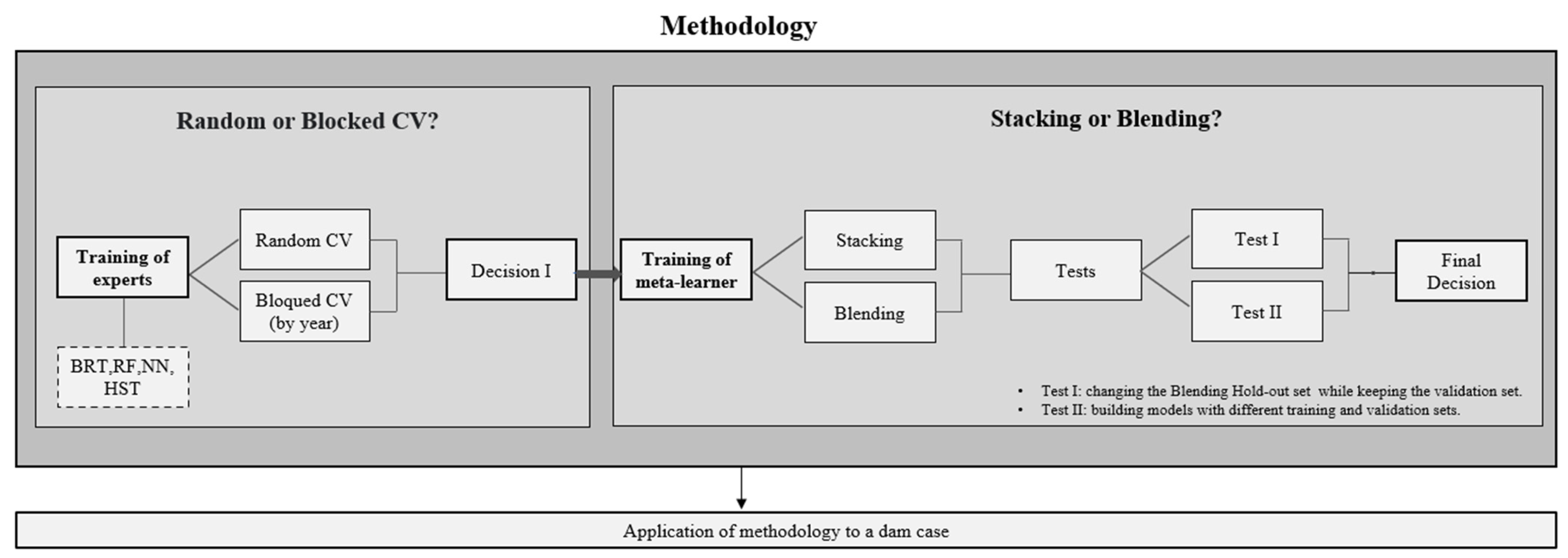
This section briefly describes the general approach to the research, with the aim of proposing a strategy to develop prediction models based on a combination of experts (Figure 1).
In the first place, the training of four experts of different algorithmic natures was executed: Boosted Regression Trees (BRT), Random Forest (RF), Neural Networks (NN), Hydrostatic-Seasonal-Time (HST). Each of these experts was trained using two different evaluation and hyperparameter optimization methods: Random and Blocked Cross Validation (CV). In this paper, each block corresponds to a different year, so the term Annual CV will appear throughout this article, referring to a Blocked CV where the blocks are years.
The errors obtained from the two processes of Cross Validation were compared for every expert. The main objective was to observe which one gave a better error estimator and prediction for future data. The strategy that yields a CV error most similar to the validation error is the appropriate estimation strategy.
On the other hand, the optimal hyperparameters of each expert obtained by both strategies were compared and their impact on the error in the validation set was analyzed. Thus, we studied which strategy, Random or Blocked CV, generates a better prediction in the validation set.
The decision made after this analysis is called “Decision I” (Figure 1) and determined which experts and which CV process should be implemented for training the second-level models of combination of experts.
The predictions of the experts chosen were used to train the second-level models through two different strategies: Stacking and Blending. The main objective of this research was to determine the best strategy and improve the accuracy of predictions.
For that purpose, two different sets of tests were performed, Test I and Test II (Figure 1). Test I consisted of changing the Blending Hold-out set while keeping the validation set. This involved training several models where the training set of each model was a different year. Therefore, it was possible to analyze the differences in the errors in the validation year, depending on the election of the training year (Hold-out set). The variance and mean of the resulting set of errors were used to determine whether Blending is an appropriate strategy or not. Test II was based on the building of models with different training and validation sets. Each training set contained different years and was used to train the experts and the meta-learner. The errors in the validation set of the second-level models, trained through the Stacking and Blending strategies, were compared to determine the best one.
The described methodology was applied to the monitoring data of radial movements of an arch dam.
2.2. Methodology
In this methodology, the experts used to build the meta-learner were chosen based on the quality of their performance and their nature. Sufficiently accurate models of different natures were selected to cover as much information as possible through their prediction vectors. Therefore, we worked with ensembles of decision trees, BRT and RF; Neural Networks, NN; and Hydrostatic-Season-Time, HST. Regarding the integrative method, meta-learners of Stacking and Blending were both built by Generalized Linear Regression. These experts were trained using external and time factors as explanatory variables, including synthetic variables derived from them, such as moving averages, aggregates, and variation rates of different orders.
2.2.1. Random or Blocked Cross Validation?
As mentioned in Section 1, the folds generated during CV are usually composed of randomly chosen instances to achieve an optimal representation of the data set. However, this method is not valid for series where there is time dependence, as is the case for dam behavior. For this reason, the need to partition in a different way arises to better represent the problem. Hence, Blocked CV, or Annual CV, where each block is a year, is introduced to optimize the hyperparameters and estimate the error in future data.
For ease of explanation, it is assumed that there are no hyperparameters to optimize. Therefore, for each split shown in Figure 2, a model is trained on the training folds and predictions are made on the test fold. Thus, we have a vector of predictions for each fold, which together add up to a number of instances, or dates, equal to the total training set. Due to the fact that we have such prediction vectors, we can calculate the error by comparing the observed and predicted values of the test fold using some error measure. The mean error made in all of these folds is the estimated error for future data.
It should be noted that, in each of these splits, the data reserved for testing have not been considered during the training phase. This fact is of utmost importance, since it allows one to use the instances corresponding to that fold to make predictions and calculate the error.
Up to this point, the Blocked CV by years has been explained to estimate the model error assuming there are no hyperparameters to optimize.
To introduce the optimization of the hyperparameters, we operate in a similar way. The main difference is that, instead of training only one model for each split, we must train as many models as there are combinations of hyperparameters. These are used to make predictions over the test fold in each split. The combination that gives the lowest mean error among folds is chosen, and its error becomes the estimated value for future data.
The same approach is taken for Random CV, but the instances in each fold are chosen randomly without replacement. In a Random CV, instances from different years can be found, whereas in the Blocked CV, used in our research, all instances necessarily belong to the same year. Decision I in Figure 1 was taken by comparing the errors estimated during Blocked and Random CV to the error in the validation set.
The error measure applied to all estimations was the Root-Mean-Square Error (RMSE), which has the following mathematical form [25]:
where is the predicted value of instance i, is the observed value of the same instance i, and m is the total number of instances.
2.2.2. Stacking or Blending?
Predictions originating from the test folds of the Blocked CV served as the training data set for the meta-learner built through the Stacking and Blending strategies. If all the available predictions are used to train the meta-learner, we speak of Stacking, while if only 10 or 20% of the data is used, we speak of Blending. The origin of both is detailed below.
We started from an m × n matrix corresponding to the training set D, where m is the number of rows, or available dates, and n the number of explanatory variables:
Assume that for each expert a Blocked CV with 5 folds, similar to Figure 2, has been used to find the optimal hyperparameters and estimate the RMSE. Thus, the training set is divided into five blocks, and predictions for each test fold are obtained, so that eventually all instances of the set are used at least once for validation. Then, the following data set shown in Table 1 is obtained:
For each fold shown in Table 1, four subsets are used for training (Train) and one subset is used for testing (Test). Train cells are green in Figure 2 and test cells are blue. The prediction vectors of each Test subset are calculated during Cross-Validation for every model. Therefore, for each expert (from 1 to ) we obtain a prediction vector that contains a total number of elements corresponding to the instances of all Test folds together (Test1, …, Test5 in Table 1), which is the same amount as that of matrix in Equation (2).
By joining these vectors to the target variable , the following training matrix is obtained:
where is prediction of the expert . The first column in Equation (3) is the prediction vector of expert 1, and so on.
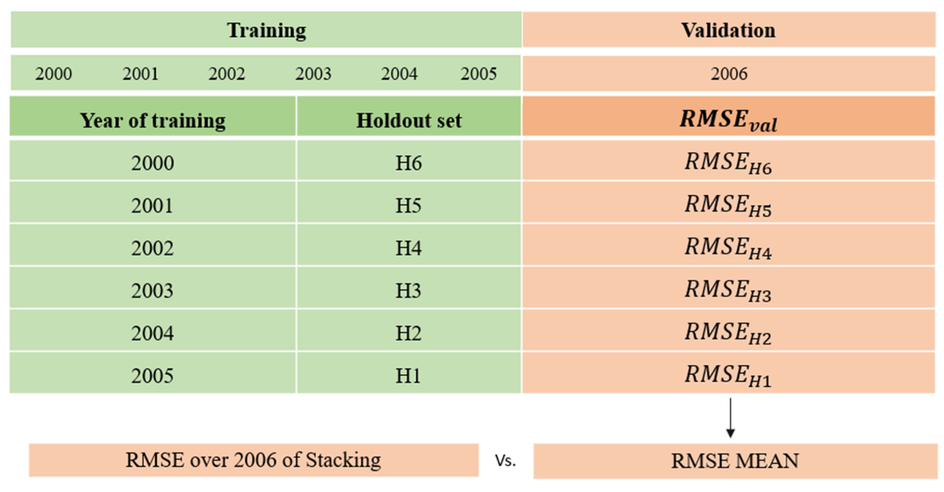
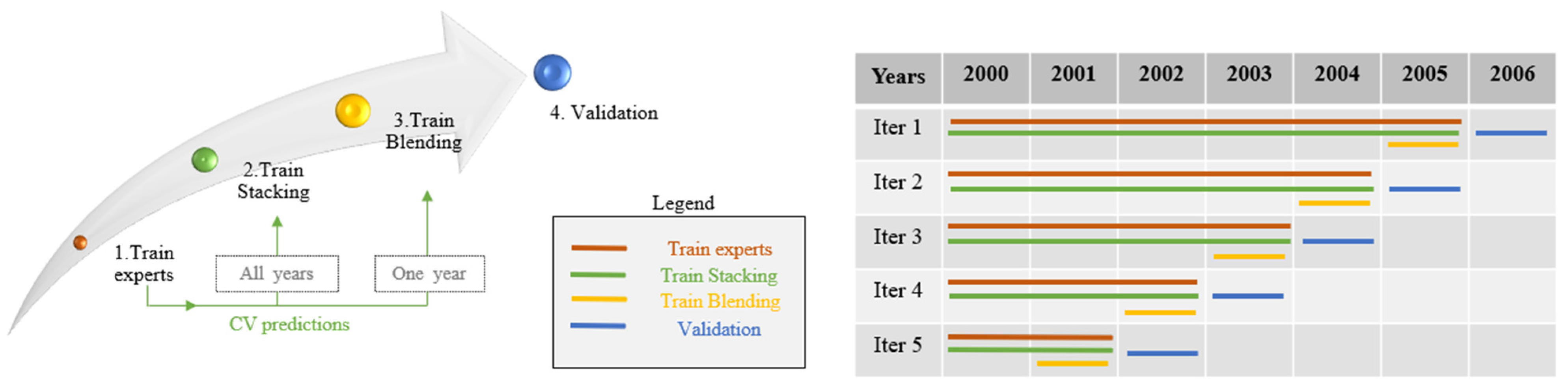
The following Figure shows a specific example where 6 years are available in the training set and there are 3 experts built:
The elements on the left of Figure 3 show what has been explained so far in matrix form. Three experts are trained on data from 2000 to 2005, where each year is one fold. The prediction vector for each year is obtained from CV and the matrix D′ is formed to train the meta-learner with Stacking strategy. The elements on the right show the number of years used for Stacking and the year used for Blending (2005), called the Hold-out set. Both the experts and the meta-learner are then validated over the validation set (2006). Thus, an error is obtained for every model built.
More generally, the matrix representing the training set of the experts is D, shown in Equation (2), while that of the Stacking-trained meta-learner is D′ (Equation (3)). The matrix representing the instances of the Blending Hold-out set is as follows:
where is the total number of instances in the training set, is the total number of experts and is the total number of instances in the last available year of the training set .
As mentioned in the previous section, two different sets of tests were performed to achieve the main goal of this research. Test I consisted of changing the Hold-out set used to train Blending meta-learners, to analyze the mean and variance of the error made over the validation set.
Figure 4 shows an example of this analysis where 6 years are available in the data set. The usual approach to train the second-level model with the Blending strategy would be using data from 2005. However, to solve the question posed, a meta-learner is trained for each available year in the training set and validated with data from 2006. Thus, it is possible to analyze the variance of the error measure as a function of the year used for its construction and compare its mean to the error made by the Stacking second-level model.
On the other hand, Test II consisted of training the experts and the Stacking and Blending meta-learners with different training sets, i.e., with a different number of years. In each case, a validation was performed in the following year of the last training set to compare both strategies.
The flow of the different training processes can be observed in the arrow shown in Figure 5. First, the experts are trained, then, the second-level model with all CV predictions (Stacking), next, the Blending meta-learner is trained with the predictions of the last year of the training set, and, finally, all models are validated. In the table of Figure 5, five different training processes are simulated, where several colored lines are drawn to represent the years used to train and validate the different models. The red color represents the training of experts; the green color represents the Stacking meta-learner; the yellow color is reserved for Blending; and the blue color for the validation year. Thus, in the first round of training, or iteration 1, the training flow is as follows:
- The experts are first trained with the data corresponding to the instances between 2000 and 2005.
- The Stacking second-level model is trained with the CV predictions of these experts, which belong to the same years as them.
- The Blending meta-learner is built with the CV predictions of the experts of the last year available in the training.
- Models are validated over the following year.
Through this methodology, we expected to achieve the objectives of this research and be able to draw solid conclusions on the best combination and Cross Validation strategy.
2.3. Dam Case: Description and Available Data
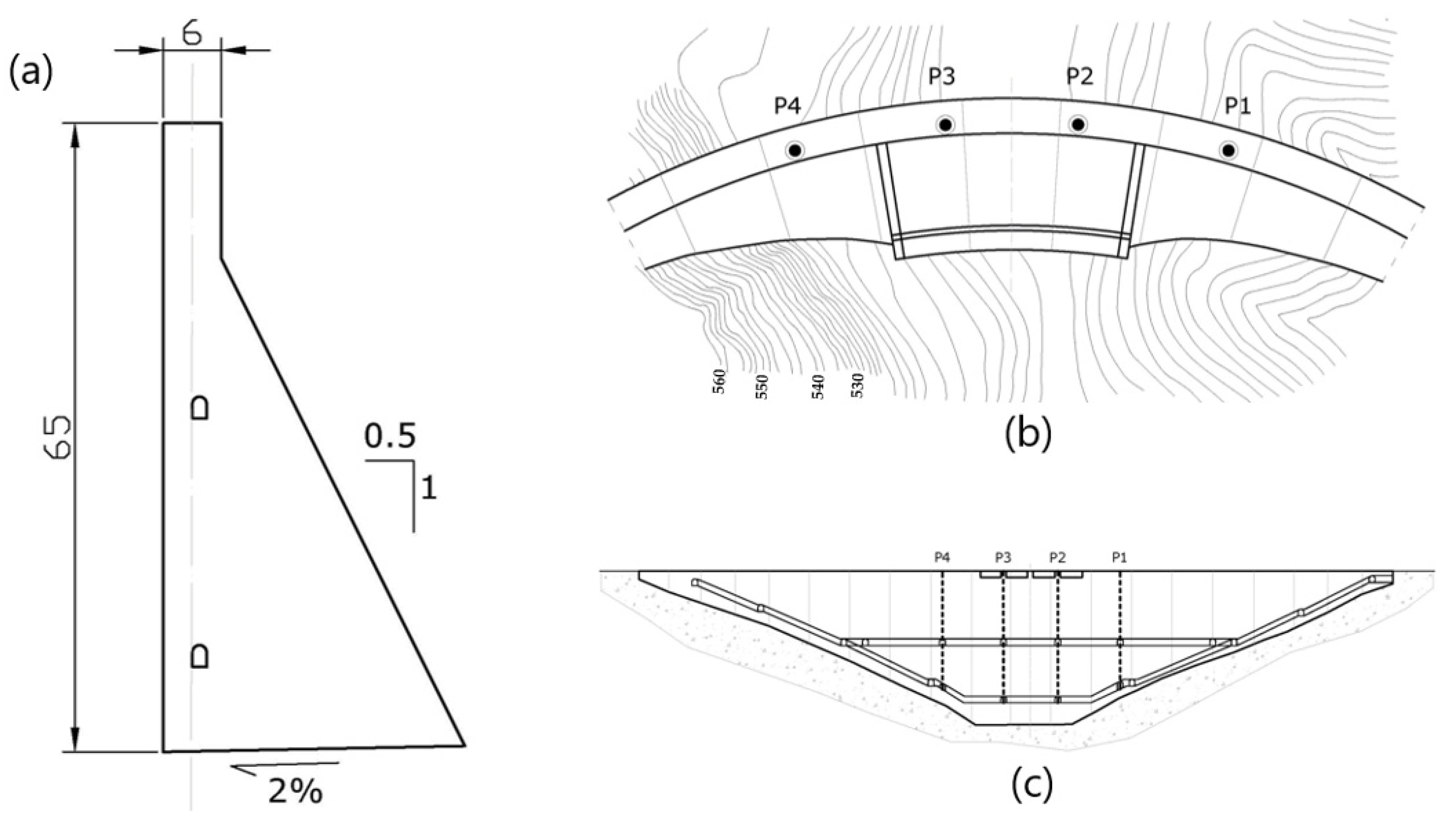
With the aim of testing the proposed methodology, data obtained from an arch-gravity dam more than 60 m high were used.
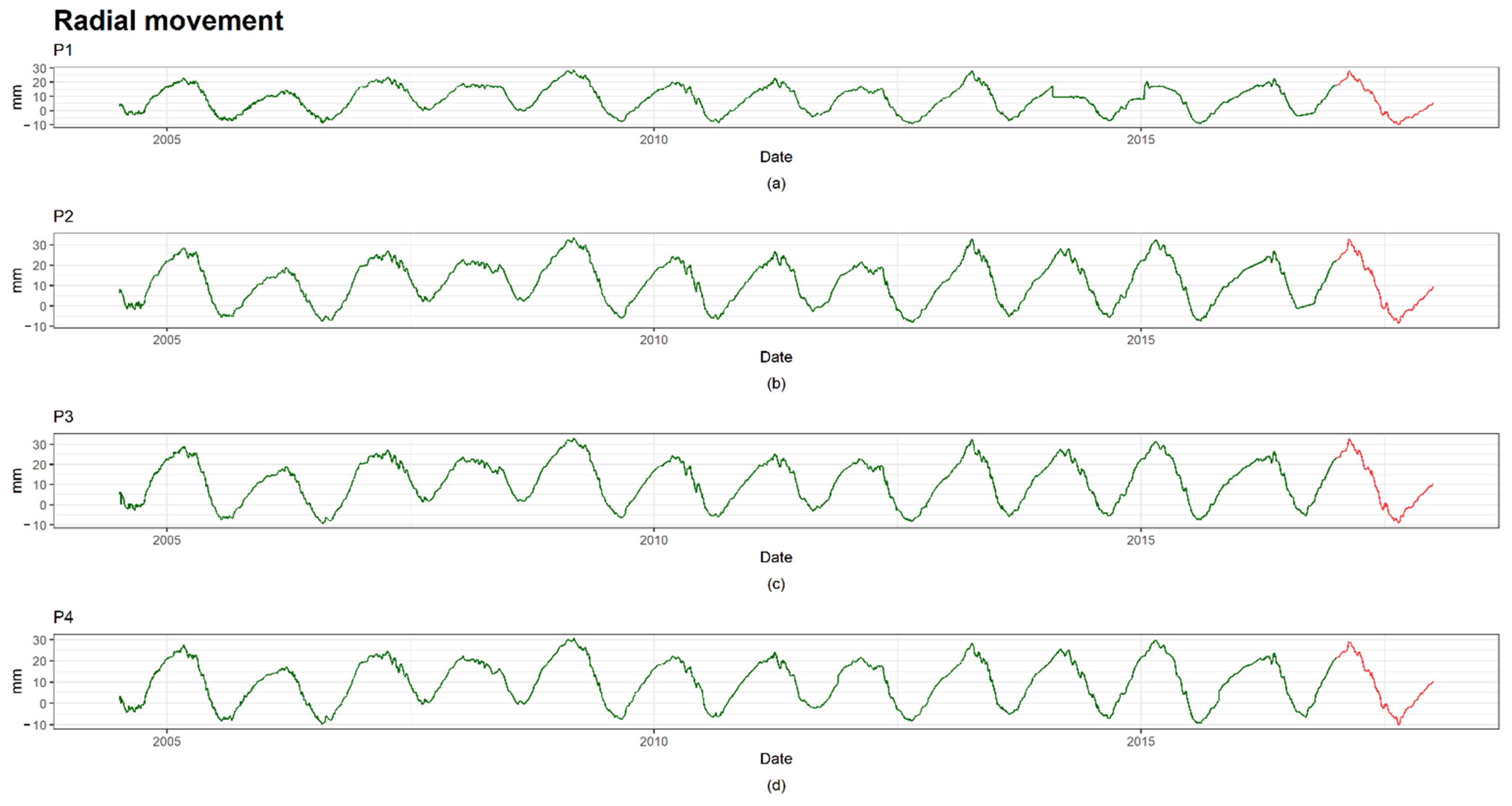
The dam is equipped with different monitoring devices, including direct pendulums. Since the displacement of the dam is a good indicator of its safety condition, the measurement of radial movement at four direct pendulums was chosen. The devices are located in the upper zone and in the horizontal gallery (Figure 6).
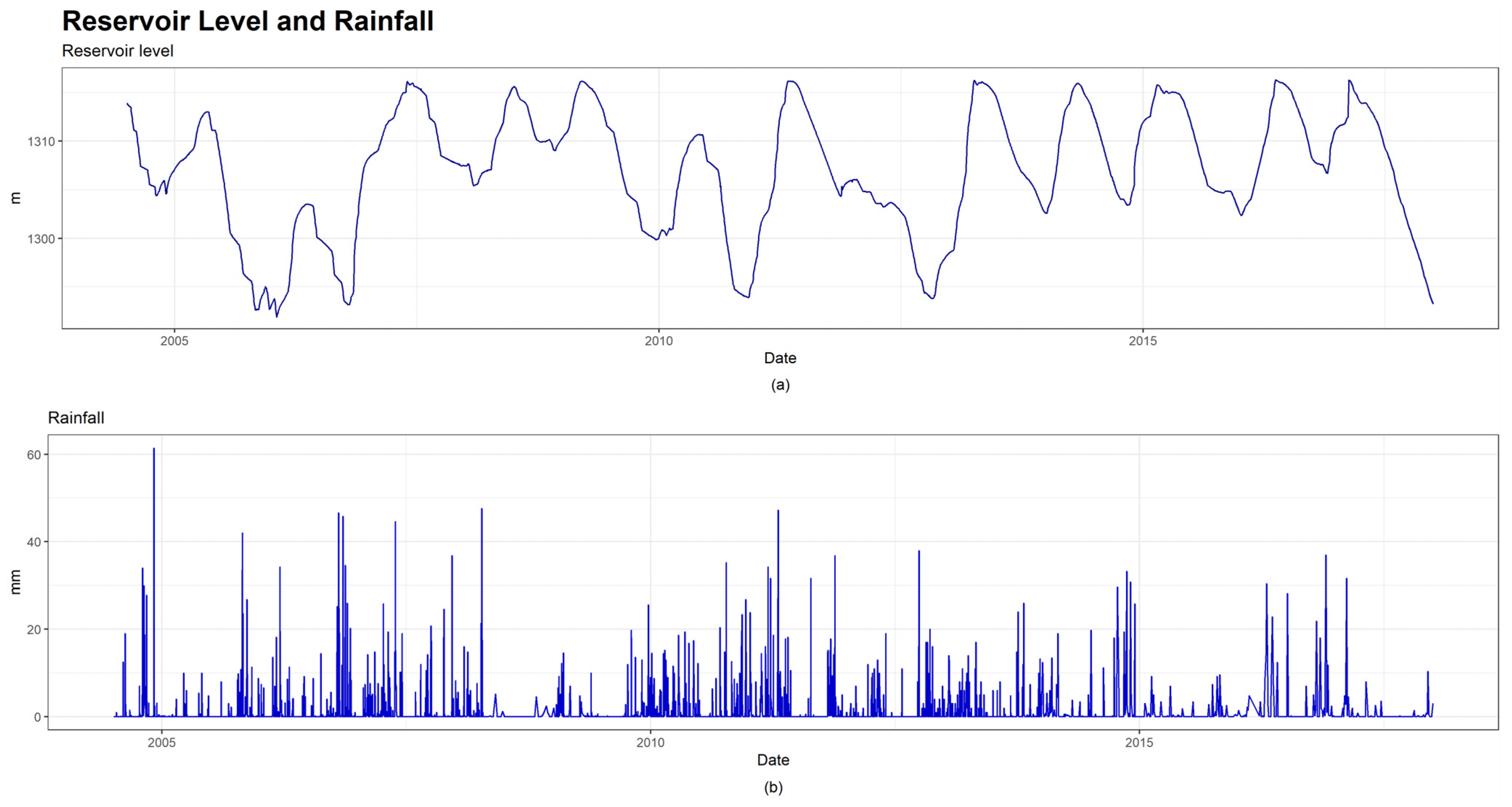
Altogether, there are approximately 3560 instances and 5 explanatory variables related to the external factors affecting the dam: maximum, minimum and mean temperature (Figure 7), reservoir level and rainfall (Figure 8). The data sets include records from 2004 to 2017. The latter was reserved as a validation set and the remaining dates were used for training (Figure 9).
3. Results and Discussion
This section presents and discusses the results obtained by applying the proposed methodology to the dam described in the previous section. It has been divided into two subsections, following the outline shown in Figure 1.
3.1. Cross Validation
Table 2 shows two different RMSE values for both strategies: RMSEcv and RMSEval. The first measures the error (RMSE) during the Cross Validation process, which is the mean of the RMSE values across folds. The second refers to the error over the validation set [24]. The third measure is the relative difference between both errors calculated by the following formula:
where .
As mentioned in previous chapters, it is more robust to use the estimated error obtained during the CV process, because it is calculated using a larger number of instances. However, the RMSE in the validation set should be compared with the RMSEcv value, seeking the smallest difference between them.
The negative values of RD in Table 2 show that the error over the validation set is higher than the one estimated by CV. All these values, except one, are negative and quite high in the case of Random CV. They fall within the range of [−578.06%, −8.26%], excluding the result of HST, which can be considered atypical. Those of Blocked CV are significantly lower, as they fall within the range of [−62.14%, 25.81%]. The mean RD of Random CV is −210.56%, while the mean RD of Blocked CV is −8.23%. Therefore, the error estimated during the Annual CV, or Blocked CV, is considered a preferable estimator for future data.
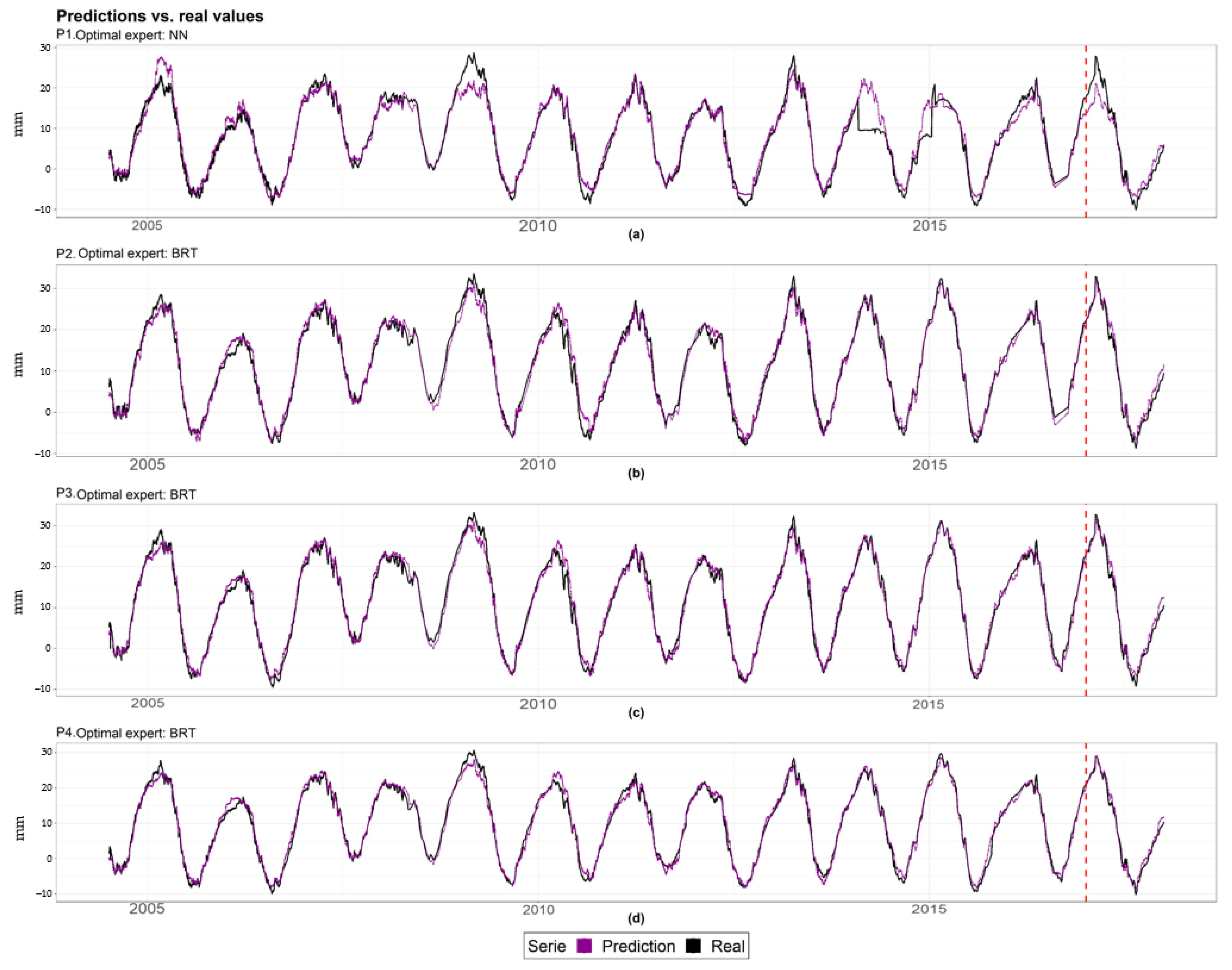
Looking at the RMSEcv values and the predictions series (Figure 10), BRT is the best expert with respect to the precision of both Random and Blocked CV in all cases, except pendulum 1, where the lowest error is reached by NN trained using the Blocked CV. The predictions of pendulum 1 (a) are less accurate in some of the peaks than those of the other pendulums. Specifically, approximately in 2014, some atypical data are detected, probably generated by a failure in the measuring device. All other experts provide significantly accurate predictions.
In addition to affecting the estimated RMSE, the choice of CV also influences the selection of hyperparameters. We use the example of the expert BRT of pendulum 4 (Table 2) to show the differences between the optimal combination of hyperparameters obtained from both processes.
Two of the hyperparameters differ between the two CV processes (Table 3)This fact, summed up in the difference between the cuts made by the ensemble trees, causes the error in the validation set to be different depending on the CV used for training.
The HST expert generates the same RMSEval regardless of the CV used (Table 2) because there are no hyperparameters to optimize. The results over the validation set of the rest of experts vary among the devices. The results shown in Table 2 indicate that Blocked CV only gives a lower RMSEval than the random approach in 4 out of the 12 cases, excluding HST. In the case of pendulums 1, 2 and 3, the RMSEval generated by Blocked CV is generally higher. However, the models of pendulum 4 are more precise when trained with such CV.
Although the RMSEval of the Random CV is lower 8 out of 12 times, the difference between the two CV types is not significantly high, between 1 and 8% in absolute value. Furthermore, considering that it is better to give an estimation where more years are included, it is convenient to use the estimated error during the CV. Since the RMSEcv of the Random CV does not serve as a good estimator for future data, as the results shown in Table 2 indicate, Annual CV is recommended as the adequate strategy to estimate the error of the model and find the optimal hyperparameters.
3.2. Experts Committee
Once the decision of applying Blocked CV to train models was taken, Decision I in Figure 1, the relevant tests were performed to determine the best strategy of combination of experts.
The results of the Test I trainings, which consist of changing the Hold-out set used to train Blending, are shown in Table 4. The column titled Training Year indicates the year used as the Hold-out set to train the Blending model. RMSEval is the error measure in the validation set: 2017. The mean and variance of these values are presented as Mean and Variance for each device, respectively. On the other hand, the error committed by the Stacking meta-learner on the same validation set is represented by RMSEvalS.
The results (Table 4) reveal that the error depends on the Hold-out set used to train the Blending meta-learner. It reaches the maximum variance in pendulum 1, with a value of 0.868. The error has lower variation in the case of pendulum 2, where the minimum variance is found.
On the other hand, the mean error of Blending meta-learners is higher than the value of RMSEvalS in most cases. It is only lower in the case of pendulum 4. However, looking at the errors made by the models trained with each Hold-out set, it is clear that Blending accuracy is higher than Stacking in most cases: 69.2% in pendulum 1, 61.5% in pendulum 3 and 76.9% in pendulum 4. Only in the case of pendulum 2 is there a lower error obtained with Stacking most of the time: 15.4% of cases.
These results were not sufficient to draw a solid conclusion on the issue addressed in this paper, although they do show the dependence of the meta-learner’s error on the Hold-out set chosen for training. Hopefully, if the training year is similar to the validation set, the error will be low. The drawback lies in the uncertainty of this fact.
Therefore, further experiments were performed with different training sets and different validation sets (Test II) to make the final decision.
The summary of the results obtained during Test II are shown in Table 5. The column named Available years indicates the number of years contained in the simulated training set. T years Stacking and experts represents the years used for the training of experts and the Stacking meta-learner. T year Blending shows the year used for Blending training, while V year is the validation set. RMSEvalS and RMSEvalB are the errors made by the Stacking and Blending meta-learners, respectively. The last column refers to the percentage improvement, reduction of the error (ER) of Stacking over Blending, calculated as follows:
The error of the meta-learner constructed through Stacking was lower than Blending in 60% of the cases, for different validation years. For pendulums 1 and 3, the error of Stacking was lower in 3 out of 5 validations (60%). In the case of pendulum 2, the maximum percentage is found, where Stacking is better in 80% of the cases. In contrast, this was met in only 40% of the validation sets in the case of pendulum 4. The results in Table 4 show that for this pendulum, Blending is better than Stacking 76.9% of the time over the validation of 2017.
The maximum advantage of Stacking over Blending is found in 2014 in pendulum 3, where the Stacking meta-learner is 36.1% better than Blending. Regarding the advantage of Blending over Stacking, its maximum is reached in the validation of 2006 in pendulum 1, where the error reduction is 47.6%.
The evident dependence of the Blending meta-learner result on the Hold-out set and the results obtained in Test II where, overall, Stacking gives a lower error, makes Stacking a more robust strategy. It might be due to the fact that Stacking strategy uses more data to train the model.
The final decision was taken, and the second-level models were finally trained following the Stacking strategy and using Blocked CV, where each block was one year.
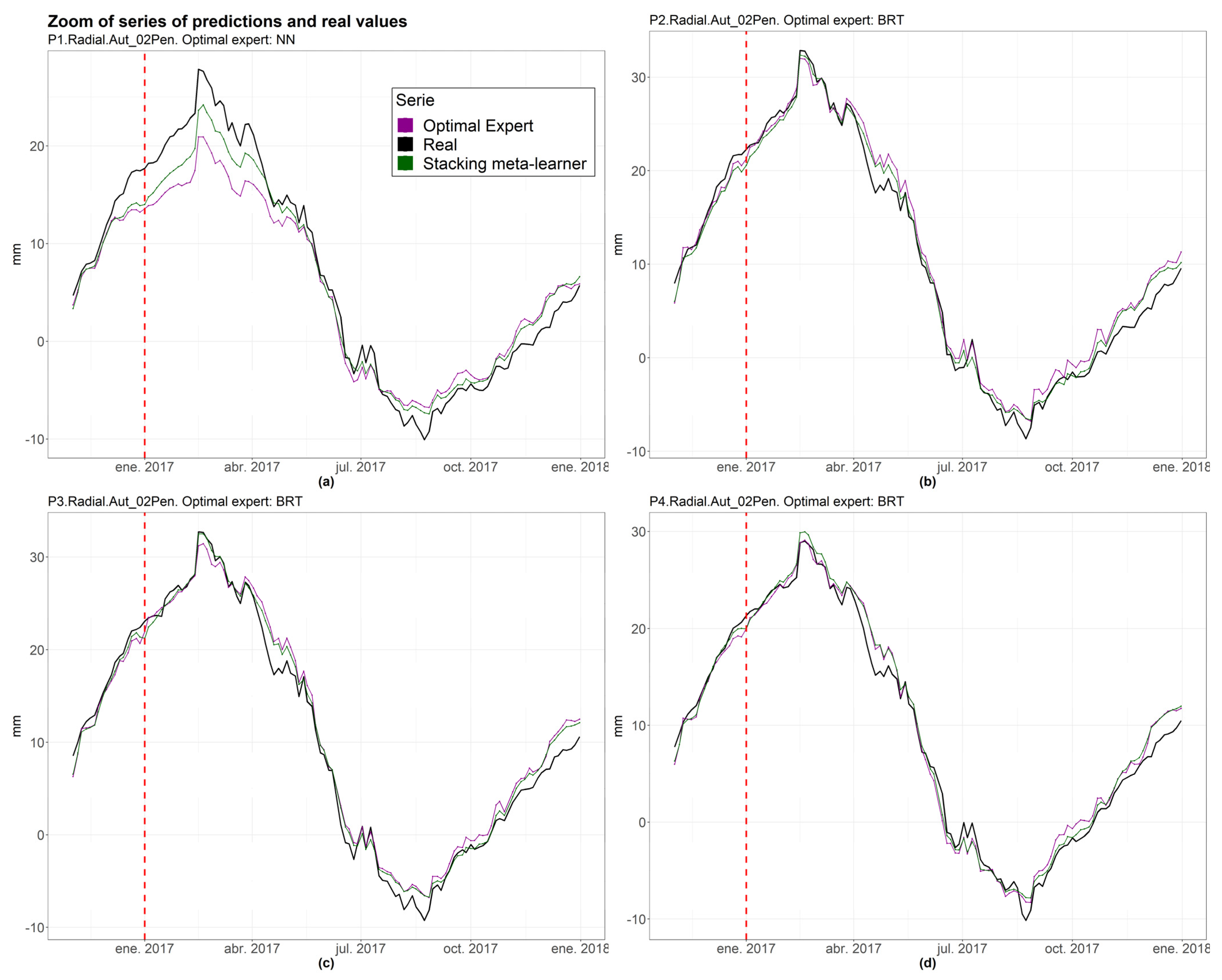
The results in Table 6 show that for all pendulums, besides pendulum 1, the meta-learner reduces the error of the optimal expert. The maximum relative difference is reached at 14.48% in pendulum 2. Furthermore, regarding individual experts, BRT achieves the greatest accuracy for all pendulums, except pendulum 1, where NN is the most precise. Figure 11 shows parts of the series where the meta-learner performs better than the best expert.
Overall, these results suggest that a combination of experts can improve the optimal expert’s precision through Stacking combination, and that Blocked CV gives the best estimate of the model error on future data compared to the random approach.
4. Conclusions
We presented a methodology that successfully combined experts to improve the accuracy and robustness of a machine learning model of the movement of a concrete dam. This paper provides new insights into the optimal strategy for performing combinations in the field of dam behavior and security. Furthermore, we highlighted the importance of the appropriate choice of the type of Cross Validation process.
Blocked CV was preferable to Random CV to estimate the model error on future data. It was observed that Random CV generates an error estimator significantly different from that obtained in the validation set, with an average difference (Equation (5)) of −210.56%, presumably due to time dependence, which makes it an unreliable strategy. On the contrary, the differences (Equation (5)) regarding Blocked CV have a mean value of −8.23%, which is significantly lower than Random CV. The RMSE values in the validation set for both types of CV are similar. Regarding the training of experts through Blocked CV, we achieved models with good prediction accuracy for all target variables, with a RMSEcv of the optimal experts lying within the range of 1.288 mm and 2.018 mm.
Stacking was considered a better strategy than Blending, since clear dependence of the Blending model on the Hold-out set used in the training was observed, with a variance value of up to 0.868 in the case of pendulum 1. Since a model trained using the Blending strategy involves using 10% or 20% of the data, the model is subject to the peculiarities of the year used in its training. The results in Table 4 emphasized that, by changing the Hold-out set in blending, the RMSE committed in the validation set significantly varies, and is higher, on average, than when adopting the Stacking strategy.
Regarding the results obtained by training experts and meta-learners on different sets and validated over different years, it was noted that the Stacking meta-learner was more accurate in most cases (60% on average). Consequently, Stacking was considered a more robust strategy for training second-level models, presumably due to superiority in the number of instances used for training.
Finally, comparing the series of predictions of the meta-learner built by generalized linear regression and the optimal expert, the second-level model improves the accuracy of the best expert in all the pendulums, with improvement percentages of up to 14.8%. Only one exception is found where accuracy is almost identical. Future research should aim to train the meta-learner through different algorithms using the Stacking strategy to determine the best meta-learner algorithm.
As a global conclusion, a methodology is proposed in which experts of different natures are trained using Blocked CV combined with a Stacking strategy.
Author Contributions
Conceptualization, P.A., M.Á.F.-C. and M.Á.T.; methodology, P.A.; software, P.A.; formal analysis, P.A., M.Á.F.-C. and M.Á.T.; investigation, P.A.; data curation, P.A.; writing—original draft preparation, P.A.; writing—review and editing, M.Á.F.-C. and M.Á.T.; visualization, P.A.; supervision, M.Á.T. All authors have read and agreed to the published version of the manuscript.
Funding
This research was funded by the project ARTEMISA (grant number RIS3-2018/L3-218), funded by the Regional Authority of Madrid (CAM) and partially funded by the European Regional Development Fund (ERDF) of the European Commission.
Institutional Review Board Statement
Not applicable.
Informed Consent Statement
Not applicable.
Data Availability Statement
The data are not available due to confidential reasons.
Acknowledgments
The authors thank Canal de Isabel II (CYII) for providing the data. In particular, we acknowledge the collaboration of David Galán from CYII.
Conflicts of Interest
The authors declare no conflict of interest.
Nomenclature
| BRT | Boosted Regression Trees |
| CV | Cross Validation |
| D | matrix representation of the data set |
| D′ | matrix form of prediction vectors of the experts |
| Di,S | relative difference between the expert (i) and the second-level model (S) |
| ER | reduction of the error of Stacking over Blending |
| GLM | Generalized Linear Regression |
| HST | Hydrostatic-Seasonal-Time |
| interactionDepth | hyperparameter of BRT that controls the depth of the tree |
| k | number of experts |
| m | number of instances of the data set |
| n | number of explanatory variables |
| nMinObsInNode | hyperparameter of BRT representing the minimum number of observations to consider in one node |
| NN | Neural Networks |
| nTree | hyperparameter of BRT representing the number of trees |
| RD | relative difference between the Rooted Squared Error over CV and the Validation set |
| RF | Random Forest |
| RMSE | Root-Mean-Square Error |
| RMSEcv | Root-Mean-Square Error over Cross Validation |
| RMSEval | Root-Mean-Square Error over validation |
| RMSEvalB | RMSE of Blending approach in Test II |
| RMSEvalS | the RMSE committed by the Stacking meta-learner in the validation set |
| shrinkage | hyperparameter of BRT that controls overfitting |
| SVM | Support Vector Machine |
References
- Hariri-Ardebili, M.A.; Pourkamali-Anaraki, F. Support vector machine based reliability analysis of concrete dams. Soil Dyn. Earthq. Eng. 2018, 104, 276–295. [Google Scholar] [CrossRef]
- Salazar, F.; Toledo, M.; Gonzalez, J.M.; Oñate, E. Early detection of anomalies in dam performance: A methodology based on boosted regression trees. Struct. Control Health Monit. 2017, 24, e2012. [Google Scholar] [CrossRef]
- Tsihrintzis, G.A.; Virvou, M.; Sakkopoulos, E.; Jain, L.C. Machine Learning Paradigms Applications of Learning and Analytics in Intelligent Systems. Available online: http://www.springer.com/series/16172 (accessed on 13 April 2021).
- Salazar, F.; Morán, R.; Toledo, M.; Oñate, E. Data-Based Models for the Prediction of Dam Behaviour: A Review and Some Methodological Considerations. Arch. Comput. Methods Eng. 2015, 24, 1–21. [Google Scholar] [CrossRef] [Green Version]
- Salazar, F.; Toledo, M.; Oñate, E.; Suárez, B. Interpretation of dam deformation and leakage with boosted regression trees. Eng. Struct. 2016, 119, 230–251. [Google Scholar] [CrossRef] [Green Version]
- Salazar, F.; González, J.M.; Toledo, M.Á.; Oñate, E. A Methodology for Dam Safety Evaluation and Anomaly Detection Based on Boosted Regression Trees. 2016. Available online: https://www.researchgate.net/publication/310608491 (accessed on 5 March 2020).
- Salazar, F.; Toledo, M.; Oñate, E.; Morán, R. An empirical comparison of machine learning techniques for dam behaviour modelling. Struct. Saf. 2015, 56, 9–17. [Google Scholar] [CrossRef] [Green Version]
- Rankovic, V.; Grujović, N.; Divac, D.; Milivojević, N. Development of support vector regression identification model for prediction of dam structural behaviour. Struct. Saf. 2014, 48, 33–39. [Google Scholar] [CrossRef]
- Mata, J. Interpretation of concrete dam behaviour with artificial neural network and multiple linear regression models. Eng. Struct. 2011, 33, 903–910. [Google Scholar] [CrossRef]
- Herrera, M.; Torgo, L.; Izquierdo, J.; Pérez-García, R. Predictive models for forecasting hourly urban water demand. J. Hydrol. 2010, 387, 141–150. [Google Scholar] [CrossRef]
- Kang, F.; Li, J.; Zhao, S.; Wang, Y. Structural health monitoring of concrete dams using long-term air temperature for thermal effect simulation. Eng. Struct. 2018, 180, 642–653. [Google Scholar] [CrossRef]
- Wolpert, D.H. Stacked generalization. Neural Netw. 1992, 5, 241–259. [Google Scholar] [CrossRef]
- Wu, T.; Zhang, W.; Jiao, X.; Guo, W.; Hamoud, Y.A. Evaluation of stacking and blending ensemble learning methods for estimating daily reference evapotranspiration. Comput. Electron. Agric. 2021, 184, 106039. [Google Scholar] [CrossRef]
- Roberts, D.R.; Bahn, V.; Ciuti, S.; Boyce, M.; Elith, J.; Guillera-Arroita, G.; Hauenstein, S.; Lahoz-Monfort, J.J.; Schroder, B.; Thuiller, W.; et al. Cross-validation strategies for data with temporal, spatial, hierarchical, or phylogenetic structure. Ecography 2017, 40, 913–929. [Google Scholar] [CrossRef]
- Bergmeir, C.; Benítez, J.M. On the use of cross-validation for time series predictor evaluation. Inf. Sci. 2012, 191, 192–213. [Google Scholar] [CrossRef]
- Džeroski, S.; Ženko, B. Is Combining Classifiers with Stacking Better than Selecting the Best One? Mach. Learn. 2004, 3, 255–273. [Google Scholar] [CrossRef] [Green Version]
- Dou, J.; Yunus, A.P.; Bui, D.T.; Merghadi, A.; Sahana, M.; Zhu, Z.; Chen, C.-W.; Han, Z.; Pham, B.T. Improved landslide assessment using support vector machine with bagging, boosting, and stacking ensemble machine learning framework in a mountainous watershed, Japan. Landslides 2019, 17, 641–658. [Google Scholar] [CrossRef]
- Mohd, L.; Gasim, S.; Ahmed, H.; Mohd, S.; Boosroh, H. Water Resources Development and Management ICDSME 2019 Proceedings of the 1st International Conference on Dam Safety Management and Engineering. Available online: http://www.springer.com/series/7009 (accessed on 13 April 2021).
- Cheng, J.; Xiong, Y. Application of Extreme Learning Machine Combination Model for Dam Displacement Prediction. Procedia Comput. Sci. 2017, 107, 373–378. [Google Scholar] [CrossRef]
- Bin, Y.; Hai-Bo, Y.; Zhen-Wei, G. A Combination Forecasting Model Based on IOWA Operator for Dam Safety Monitoring. In Proceedings of the 2013 5th Conference on Measuring Technology and Mechatronics Automation, ICMTMA 2013, Hong Kong, China, 16–17 January 2013; pp. 5–8. [Google Scholar] [CrossRef]
- Wei, B.; Yuan, D.; Li, H.; Xu, Z. Combination forecast model for concrete dam displacement considering residual correction. Struct. Health Monit. 2017, 18, 232–244. [Google Scholar] [CrossRef]
- Wei, B.; Yuan, D.; Xu, Z.; Li, L. Modified hybrid forecast model considering chaotic residual errors for dam deformation. Struct. Control Health Monit. 2018, 25, e2188. [Google Scholar] [CrossRef]
- Hong, J.; Lee, S.; Bae, J.H.; Lee, J.; Park, W.J.; Lee, D.; Kim, J.; Lim, K.J. Development and Evaluation of the Combined Machine Learning Models for the Prediction of Dam Inflow. Water 2020, 12, 2927. [Google Scholar] [CrossRef]
- Pedregosa, F.; Varoquaux, G.; Gramfort, A.; Michel, V.; Thirion, B.; Grisel, O.; Blondel, M.; Prettenhofer, P.; Weiss, R.; Dubourg, V.; et al. Scikit-learn: Machine learning in Python. J. Mach. Learn. Res. 2011, 12, 2825–2830. [Google Scholar]
- Chai, T.; Draxler, R.R. Root mean square error (RMSE) or mean absolute error (MAE)?—Arguments against avoiding RMSE in the literature. Geosci. Model Dev. 2014, 7, 1247–1250. [Google Scholar] [CrossRef] [Green Version]
- Berrar, D. Cross-Validation. In Encyclopedia of Bioinformatics and Computational Biology: ABC of Bioinformatics; Elsevier: Amsterdam, The Netherlands, 2018; Volume 1–3, pp. 542–545. [Google Scholar] [CrossRef]
Figure 1.
Summary of the methodology.

Figure 2.
Five-fold Cross Validation, where each fold coincides with an available year. The green color represents the subdivisions for model training, while the blue color represents the test subsets. The validation set is orange in color [24].
Figure 2.
Five-fold Cross Validation, where each fold coincides with an available year. The green color represents the subdivisions for model training, while the blue color represents the test subsets. The validation set is orange in color [24].

Figure 3.
Origin of the data set used to train the Stacking and Blending meta-learners.

Figure 4.
Test I with 6 years available in the data set. RMSEval is the error over the validation set (2006) and RMSEHi is the error made by the model trained with the Hold-out set Hi.
Figure 4.
Test I with 6 years available in the data set. RMSEval is the error over the validation set (2006) and RMSEHi is the error made by the model trained with the Hold-out set Hi.

Figure 5.
Test II. The arrow on the left indicates the training flow: experts, Stacking, Blending and validation. The table placed on the right points out the years used to train and validate each model.
Figure 5.
Test II. The arrow on the left indicates the training flow: experts, Stacking, Blending and validation. The table placed on the right points out the years used to train and validate each model.

Figure 6.
Cross-section (a), Plan (b) and section (c) of the dam. The source of this figure relies on information from the project that has funded this research, called ARTEMISA.
Figure 6.
Cross-section (a), Plan (b) and section (c) of the dam. The source of this figure relies on information from the project that has funded this research, called ARTEMISA.

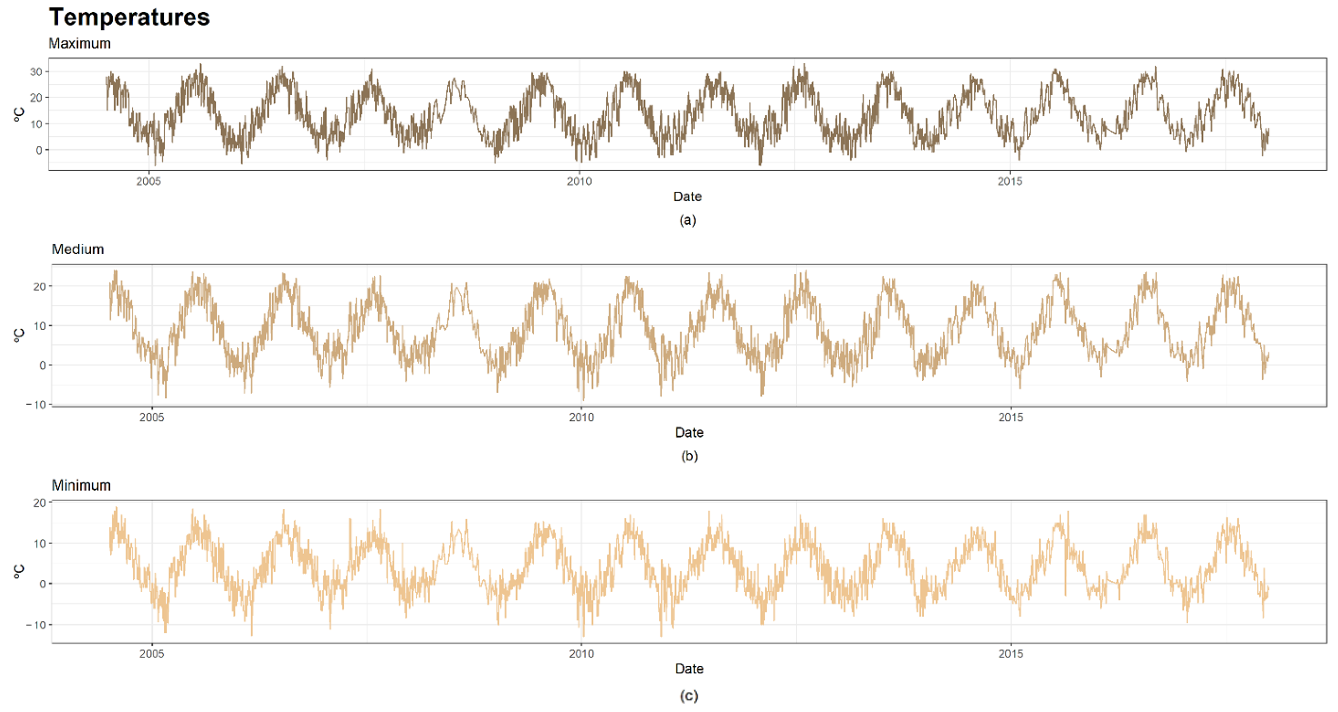
Figure 7.
Series of temperatures. (a) Series of maximum temperature; (b) Series of medium temperature; (c) Series of minimum temperature.
Figure 7.
Series of temperatures. (a) Series of maximum temperature; (b) Series of medium temperature; (c) Series of minimum temperature.

Figure 8.
Series of reservoir level and rainfall. (a) Series of reservoir level; (b) Series of rainfall.
Figure 8.
Series of reservoir level and rainfall. (a) Series of reservoir level; (b) Series of rainfall.

Figure 9.
Series of direct pendulums. Training instances are colored in green and validation dates are colored in red. (a) Series of pendulum 1; (b) Series of pendulum 2; (c) Series of pendulum 3; (d) Series of pendulum 4.
Figure 9.
Series of direct pendulums. Training instances are colored in green and validation dates are colored in red. (a) Series of pendulum 1; (b) Series of pendulum 2; (c) Series of pendulum 3; (d) Series of pendulum 4.

Figure 10.
Series of predictions (magenta color) vs. series of measured values (black color) for each target. The red dashed line separates the training (left) and validation (right) periods. (a) Series of predictions of pendulum 1; (b) Series of predictions of pendulum 2; (c) Series of predictions of pendulum 3; (d) Series of predictions of pendulum 4.

Figure 11.
Zoom series of the optimal expert, the real value and the Stacking meta-learner. The red dashed line indicates the first date of validation. (a) Zoom series of pendulum 1; (b) Zoom series of pendulum 2; (c) Zoom series of pendulum 3; (d) Zoom series of pendulum 4.
Figure 11.
Zoom series of the optimal expert, the real value and the Stacking meta-learner. The red dashed line indicates the first date of validation. (a) Zoom series of pendulum 1; (b) Zoom series of pendulum 2; (c) Zoom series of pendulum 3; (d) Zoom series of pendulum 4.


Table 1.
Representation of the data set by train and test folds in tabular form [26].
Table 1.
Representation of the data set by train and test folds in tabular form [26].
| Split | Fold 1 | Fold 2 | Fold 3 | Fold 4 | Fold 5 |
|---|---|---|---|---|---|
| 1 | Test1 | Train | Train | Train | Train |
| 2 | Train | Test2 | Train | Train | Train |
| 3 | Train | Train | Test3 | Train | Train |
| 4 | Train | Train | Train | Test4 | Train |
| 5 | Train | Train | Train | Train | Test5 |
Table 2.
Prediction errors for both strategies: Random and Blocked Cross Validation.
| Pendulum | Expert | RMSEcv | RMSEval | RD | |||
|---|---|---|---|---|---|---|---|
| Random CV | Blocked CV | Random CV | Blocked CV | Random CV | Blocked CV | ||
| 1 | BRT | 0.435 | 2.2 | 2.522 | 2.331 | −479.77% | −5.95% |
| HST | 2.113 | 2.848 | 2.113 | 2.113 | 0.00% | 25.81% | |
| NN | 1.397 | 2.018 | 3.254 | 3.272 | −132.93% | −62.14% | |
| RF | 0.506 | 2.649 | 3.431 | 3.494 | −578.06% | −31.90% | |
| 2 | BRT | 0.346 | 1.404 | 1.487 | 1.596 | −329.20% | −13.65% |
| HST | 1.853 | 2.080 | 2.249 | 2.249 | −21.38% | −8.15% | |
| NN | 0.933 | 1.446 | 1.359 | 1.385 | −45.58% | 4.22% | |
| RF | 0.437 | 1.925 | 2.073 | 2.117 | −374.77% | −9.98% | |
| 3 | BRT | 0.368 | 1.288 | 1.478 | 1.587 | −301.63% | −23.21% |
| HST | 2.224 | 2.438 | 2.433 | 2.433 | −9.40% | 0.21% | |
| NN | 0.884 | 1.473 | 1.316 | 1.367 | −48.87% | 7.20% | |
| RF | 0.439 | 1.832 | 2.015 | 1.998 | −359.00% | −9.06% | |
| 4 | BRT | 0.361 | 1.299 | 1.433 | 1.314 | −296.95% | −1.15% |
| HST | 2.203 | 2.436 | 2.385 | 2.385 | −8.26% | 2.09% | |
| NN | 0.882 | 1.416 | 1.35 | 1.371 | −53.06% | 3.18% | |
| RF | 0.426 | 1.652 | 1.832 | 1.805 | −330.05% | −9.26% | |
Table 3.
Optimal hyperparameters of BRT found by Random and Blocked CV. NTree is the number of trees, nMinObsInNode is the minimum number of observations to consider in one node, shrinkage controls, overfitting and interaction depth control the tree depth.
Table 3.
Optimal hyperparameters of BRT found by Random and Blocked CV. NTree is the number of trees, nMinObsInNode is the minimum number of observations to consider in one node, shrinkage controls, overfitting and interaction depth control the tree depth.
| CV Type | nTree | InteractionDepth | Shrinkage | nMinObsInNode |
|---|---|---|---|---|
| Random | 5000 | 8 | 0.01 | 5 |
| Blocked | 5000 | 2 | 0.01 | 15 |
Table 4.
Results of Test I, which consists of changing the training Hold-out set of Blending models.
Table 4.
Results of Test I, which consists of changing the training Hold-out set of Blending models.
| Training Year | RMSEval | |||
|---|---|---|---|---|
| Pendulum 1 | Pendulum 2 | Pendulum 3 | Pendulum 4 | |
| 2004 | 4.184 | 2.524 | 2.866 | 2.175 |
| 2005 | 1.342 | 1.257 | 1.090 | 1.203 |
| 2006 | 1.843 | 1.28 | 1.215 | 0.581 |
| 2007 | 2.232 | 1.622 | 1.611 | 1.534 |
| 2008 | 1.775 | 1.527 | 1.167 | 1.181 |
| 2009 | 1.793 | 1.583 | 1.313 | 1.168 |
| 2010 | 1.416 | 1.611 | 1.098 | 1.720 |
| 2011 | 1.485 | 1.357 | 1.021 | 0.576 |
| 2012 | 2.505 | 1.447 | 1.351 | 0.750 |
| 2013 | 3.336 | 1.086 | 0.937 | 0.810 |
| 2014 | 1.495 | 1.126 | 0.960 | 0.757 |
| 2015 | 1.112 | 1.213 | 0.902 | 1.198 |
| 2016 | 1.967 | 1.309 | 1.412 | 0.974 |
| Mean | 2.037 | 1.457 | 1.303 | 1.125 |
| Variance | 0.868 | 0.367 | 0.513 | 0.469 |
| RMSEvalS | 2.035 | 1.1813 | 1.257 | 1.257 |
Table 5.
Results of Test II, which consists of training the experts, Stacking and Blending meta-learners, with different training sets. Positive values of ER imply a lower error on the Stacking meta-learner than Blending.
Table 5.
Results of Test II, which consists of training the experts, Stacking and Blending meta-learners, with different training sets. Positive values of ER imply a lower error on the Stacking meta-learner than Blending.
| Pendulum | Available Years | T years Stacking and Experts | T Year Blending | V Year | RMSEvalS | RMSEvalB | ER |
|---|---|---|---|---|---|---|---|
| 1 | 3 years: [2004–2006] | 2 years: [2004–2005] | 2005 | 2006 | 2.443 | 1.655 | −47.6% |
| 5 years: [2004–2008] | 4 years: [2004–2007] | 2007 | 2008 | 0.960 | 0.988 | 2.8% | |
| 6 years: [2004–2009] | 5 years: [2004–2008] | 2008 | 2009 | 1.454 | 1.317 | −10.4% | |
| 11 years: [2004–2014] | 10 years: [2004–2013] | 2013 | 2014 | 6.864 | 7.444 | 7.8% | |
| 13 years: [2004–2016] | 12 years: [2004–2015] | 2015 | 2016 | 3.171 | 3.330 | 4.8% | |
| 2 | 3 years: [2004–2006] | 2 years: [2004–2005] | 2005 | 2006 | 23.830 | 28.095 | 15.2% |
| 5 years: [2004–2008] | 4 years: [2004–2007] | 2007 | 2008 | 1.389 | 1.152 | −20.6% | |
| 6 years: [2004–2009] | 5 years: [2004–2008] | 2008 | 2009 | 1.948 | 2.714 | 28.2% | |
| 11 years: [2004–2014] | 10 years: [2004–2013] | 2013 | 2014 | 1.232 | 1.435 | 14.1% | |
| 13 years: [2004–2016] | 12 years: [2004–2015] | 2015 | 2016 | 1.055 | 1.157 | 8.8% | |
| 3 | 3 years: [2004–2006] | 2 years: [2004–2005] | 2005 | 2006 | 3.736 | 3.488 | −7.1% |
| 5 years: [2004–2008] | 4 years: [2004–2007] | 2007 | 2008 | 0.908 | 0.974 | 6.8% | |
| 6 years: [2004–2009] | 5 years: [2004–2008] | 2008 | 2009 | 1.393 | 1.139 | −22.4% | |
| 11 years: [2004–2014] | 10 years: [2004–2013] | 2013 | 2014 | 1.048 | 1.639 | 36.1% | |
| 13 years: [2004–2016] | 12 years: [2004–2015] | 2015 | 2016 | 1.238 | 1.347 | 8.1% | |
| 4 | 3 years: [2004–2006] | 2 years: [2004–2005] | 2005 | 2006 | 3.024 | 2.412 | −25.4% |
| 5 years: [2004–2008] | 4 years: [2004–2007] | 2007 | 2008 | 0.892 | 0.797 | −11.9% | |
| 6 years: [2004–2009] | 5 years: [2004–2008] | 2008 | 2009 | 1.433 | 2.096 | 31.6% | |
| 11 years: [2004–2014] | 10 years: [2004–2013] | 2013 | 2014 | 1.094 | 0.954 | −14.7% | |
| 13 years: [2004–2016] | 12 years: [2004–2015] | 2015 | 2016 | 1.088 | 1.241 | 12.3% |
Table 6.
Results of experts and meta-learners trained through Stacking strategy and Blocked CV. Di,S is the relative difference between the expert (i) and the second-level model (S).
Table 6.
Results of experts and meta-learners trained through Stacking strategy and Blocked CV. Di,S is the relative difference between the expert (i) and the second-level model (S).
| Pendulum | 1 | ||||
| Model | BRT | NN | RF | HST | Meta-Learner |
| RMSEcv | 2.200 | 2.018 | 2.649 | 2.848 | 2.019 |
| Di,S | −9.02% | 0.00% | −31.27% | −41.13% | −0.05% |
| 2 | |||||
| Model | BRT | NN | RF | HST | Meta-Learner |
| RMSEcv | 1.404 | 1.446 | 1.925 | 2.080 | 1.201 |
| Di,S | 0.00% | −2.97% | −37.07% | −48.08% | 14.48% |
| 3 | |||||
| Model | BRT | NN | RF | HST | Meta-Learner |
| RMSEcv | 1.288 | 1.473 | 1.832 | 2.438 | 1.174 |
| Di,S | 0.00% | −14.36% | −42.24% | −89.29% | 8.85% |
| 4 | |||||
| Model | BRT | NN | RF | HST | Meta-Learner |
| RMSEcv | 1.299 | 1.416 | 1.652 | 2.436 | 1.223 |
| Di,S | 0.00% | −9.01% | −27.17% | −87.53% | 5.85% |
Publisher’s Note: MDPI stays neutral with regard to jurisdictional claims in published maps and institutional affiliations. |
© 2022 by the authors. Licensee MDPI, Basel, Switzerland. This article is an open access article distributed under the terms and conditions of the Creative Commons Attribution (CC BY) license (https://creativecommons.org/licenses/by/4.0/).
Share and Cite
MDPI and ACS Style
Alocén, P.; Fernández-Centeno, M.Á.; Toledo, M.Á. Prediction of Concrete Dam Deformation through the Combination of Machine Learning Models. Water 2022, 14, 1133. https://doi.org/10.3390/w14071133
AMA Style
Alocén P, Fernández-Centeno MÁ, Toledo MÁ. Prediction of Concrete Dam Deformation through the Combination of Machine Learning Models. Water. 2022; 14(7):1133. https://doi.org/10.3390/w14071133
Chicago/Turabian StyleAlocén, Patricia, Miguel Á. Fernández-Centeno, and Miguel Á. Toledo. 2022. "Prediction of Concrete Dam Deformation through the Combination of Machine Learning Models" Water 14, no. 7: 1133. https://doi.org/10.3390/w14071133
Note that from the first issue of 2016, this journal uses article numbers instead of page numbers. See further details here.