Estimating Evapotranspiration of Screenhouse Banana Plantations Using Artificial Neural Network and Multiple Linear Regression Models

Abstract

Measured evapotranspiration (LE) of screenhouse banana plantations was utilized to derive and compare two types of machine-learning models: artificial neural network (ANN) and multiple linear regression (MLR). The measurements were conducted by eddy-covariance systems and meteorological sensors in two similar screenhouse banana plantations during two consecutive seasons, 2016 and 2017. Most of the study focused on the season of 2017, which includes a more extended data set (141 days) than 2016 (52 days). The results show that in most cases, the ANN model was superior to MLR. When trained and validated over the whole data set of 2017, the ANN and MLR models provided R² of 0.92 and 0.89, RMSE of 37.5 and 45.1 W m⁻² and MAE of 21 and 27.2 W m⁻², respectively. Models could be derived using a training dataset as short as one month and still provide reliable estimations. Depending on the chosen calendar month for training, R² of the ANN model varied in the range 0.81–0.89, while for the MLR model, it ranged 0.73–0.88. When trained using a data set as short as one week, there was some deterioration in model performance; the corresponding ranges of R² for the ANN and MLR models were 0.37–0.89 and 0.37–0.71, respectively. As expected for a screenhouse decoupled environment, solar radiation (Rg) was the variable that most influenced LE; using Rg as the sole input variable, the ANN model resulted in R², RMSE and MAE of 0.88 and 47 W m⁻² and 25.6 W m⁻², respectively, values that are not much worse than using all input variables (solar radiation, air temperature, air relative humidity and wind speed). Using Rg alone as the input to the MLR model only slightly deteriorated R² (=0.88); however, RMSE (=124 W m⁻²) and MAE (=75.7 W m⁻²) were significantly larger compared to a model based on all input variables. To examine model performance in different seasons, models were trained using the data set of 2017 and validated in 2016, and vice versa. Results showed that training on the data of 2017 and validation in 2016 provided superior results than the opposite, presumably since the 2017 measurement season was longer and weather conditions were more diverse than in the 2016 data set. It is concluded that the ANN and MLR models are reasonable options for estimating evapotranspiration in a banana screenhouse.

1. Introduction

Crop evapotranspiration (ETc, also denoted as LE) represents the rate of water vapour loss to the atmosphere from plants (transpiration) and soil (evaporation). Hence, sound knowledge of ETc is vital for hydrological and weather modelling, water resources management, and irrigation decision-making.

Crop evapotranspiration can be determined using different approaches. In modern agricultural practice, the recommended method estimates the reference evapotranspiration, ET₀, from standard meteorological data and multiplies it by a crop coefficient [1]. The most common method for estimating ET₀ is the Penman-Monteith (PM) FAO56 equation [1]. This method considers ET₀ as the evapotranspiration from a well-irrigated hypothetical grass, uniformly covering an infinite horizontal flat surface. Field experiments determine the crop coefficient empirically, and corresponding tables are available for many conventional crops worldwide [1].

The PM-FAO56 approach is quite simple since it can determine ET₀ from a standard meteorological station near the field of interest. Therefore, this approach became highly popular among growers. However, unavoidable differences between the local crop microclimate and that measured by a nearby weather station may cause significant inaccuracies in estimating ETc from ET₀. Moreover, the tabulated crop coefficient data are based on average conditions and may not accurately represent the plants’ specific status. Another approach for estimating ETc applies the Penman-Monteith equation, using local microclimate data and crop-specific aerodynamic and surface resistances. This method can provide reliable data on actual ETc; for example, Katerji and Rana [2] showed that estimating ETc by the Penman-Monteith equation provided more accurate data than the PM-FAO56 for six irrigated crops under Mediterranean conditions. However, this approach requires crop-specific data that is not always easy to collect under routine field operations.

Another modelling approach that has become more and more popular in the research community utilizes machine learning methods. In these models, a target value of ETc is determined, either through direct measurement or through the PM-FAO56 approach. Then, a set of input meteorological and crop variables corresponding to the target value is used to train a system that builds a mathematical function connecting the input variables and the target. The output obtained from this function is compared with actual data, and the network fine-tunes the function until it provides an estimate with satisfactory accuracy. This stage is called either training or learning. In the validation stage that follows the learning, input meteorological values that were not included in the training phase are used, and the estimated ETc is compared against measured values. Usually, R², RMSE (root mean square error) and MAE (mean absolute error) of a linear regression between calculated and measured daily or half-hourly ETc values are used to evaluate the model’s performance.

A popular model of the above type is the artificial neural network (ANN). This non-linear statistical technique resembles the human brain’s neural network in building the mathematical relations among input variables and the target. The system consists of input and output layers with intermediate hidden layers, each with several neurons [3].

Several studies examined the ANN model for estimating the reference evapotranspiration, ET₀. In the study by Zanetti et al. [4], the main goal was to evaluate the model’s performance using minimum input climate data. Their analysis used data from two standard meteorological stations in Brazil. The results showed good agreement between ET₀ estimated by ANN and by the PM-FAO56 method. Moreover, they showed that using only the minimum and maximum daily air temperatures as input variables, satisfactory results of ET₀ could be obtained. An approach combining a neural network (NN) and fuzzy logic (FL) for estimating ET₀ was also examined [5]. The input data included daily solar radiation, relative humidity, air temperature, and wind speed, collected from a wide variety of climates. They [5] showed that the combined new approach (NN + FL) was in better agreement with evapotranspiration measured from a grass-covered lysimeter that simulated ET₀ than the traditional PM-FAO56 model. Laaboudi et al. [3] examined the effectiveness of artificial neural networks (ANNs) for evaluating ET₀, using data of meteorological stations in the region of Adrar Province, Algeria. They analysed different neural network structures and found that the network with two hidden layers and eight neurons per layer provided the best results. Manikumari et al. [6] used the deep learning neural network (DLNN) methodology to estimate ET₀ in India’s rice cultivation region, using climatic conditions from standard meteorological stations. This study showed superior performance of the DLNN model over other types of ANN models and the PM-FAO56. Deep learning methods were also examined by Chen et al. [7], who examined three DL models, namely, deep neural networks (DNNs), temporal convolution neural networks (TCNs) and long short-term memory neural network (LSTMs) to estimate daily reference evapotranspiration with incomplete meteorological data. Their results showed that generally, the methods examined outperformed classical empirical models for estimating ET₀. Tikhamarine et al. [8] examined five novel hybrid machine-learning approaches to estimating monthly reference evapotranspiration in two different regions: India and Algeria. Results showed that the model ANN-GWO (ANN-grey wolf optimizer) provided better results than the others using five input variables: min/max temperature, relative humidity, wind speed and solar radiation. Satisfactory results were also obtained by these models using only three input variables: min/max temperature and solar radiation.

The above studies used an ANN to estimate the reference evapotranspiration, ET₀, not the actual one, ETc. Kelley et al. [9] used the eddy-covariance method to measure ETc over various field crops. An ANN was trained to estimate ETc utilizing the output from nearby standard meteorological sensors. Results of the ANN prediction were in accord with those calculated by the PM equation under most conditions. In a more recent study, actual crop evapotranspiration, ETc, from vegetable beans and hazelnuts was measured by eddy-covariance and estimated by ANN [10]. Results showed that this approach robustly estimated ETc using input data of the four major climatic variables: air temperature, solar radiation, air humidity, and wind speed, and a training period as short as one week. Chen et al. [11] used a temporal convolution network (TCN), which is a new form of convolution neural network, to predict daily ETc of maize under mulched drip irrigation conditions. The data were collected in a two-year field study with lysimeters. Predictions were also used to estimate the crop coefficient and compare it with literature data (FAO-56) for maize. The results [11] suggested that the seven variables of plant height, mean temperature, maximal temperature, relative humidity, solar radiation, leaf area index and soil temperature mostly affected maize evapotranspiration. The TCN model predicted daily ETc with R² and MSE in the ranges 0.91–0.95 and 0.144–0.296 mm d⁻¹ respectively. A comparative study of different machine learning algorithms was carried out by Granata [12]. The models predicted actual evapotranspiration from grass pastures at a Central Florida site, using different combinations of the input variables. Actual evapotranspiration measurements were done by the eddy covariance method. The study [12] concluded that it is possible to build a reliable machine-learning model to predict ETc with mean temperature, net radiation and relative humidity as input variables.

Another method within the machine learning family is multiple linear regression (MLR). The method assumes a linear relationship between each of the input variables and the target. The model adjusts the coefficients of the linear functions to obtain satisfactory accuracy in the estimation of the target. Laaboudi et al. [3] compared the performance of ANN and MLR on the same data set and demonstrated the superiority of ANN in predicting ET₀. For example, during the validation phase, R² for ANN and MLR were 1.00 and 0.95, while corresponding values of RMSE were 0.17 and 0.49 mm day⁻¹, respectively. Adamala [13] compared ANN and MLR in estimating daily ET₀ from data of 15 meteorological stations in India. Their results showed that ANN models performed better than the MLR models for 14 out of the 15 locations. This finding was confirmed by both higher values of R² and lower values of RMSE (mm day⁻¹).

ANN and MLR models’ performance was also compared in estimating evaporation from water reservoirs. Although evaporation is not precisely the same process as evapotranspiration, both describe similar physical processes of water phase change from liquid to vapour and water vapour transport from the biosphere to the atmosphere. For example, Deswal and Pal [14] made such a comparison and indicated that ANN performed better than MLR in evaporation predictions.

Undoubtedly, the actual routine measurement of ETc is preferable over modelling and could provide more reliable data for irrigation management. Measurement techniques are based on soil, plant, or atmospheric approaches. One popular method is the lysimeter, which measures water vapor loss from a potted plant [15]. In this method, soil evaporation and plant transpiration are monitored through the temporal change in the pot weight. Another method is the heat-pulse [16,17], which measures transpiration only based on quantifying the sap flow rate in plant stems. Under conditions of low evaporation, e.g., when plant cover fraction is high, transpiration can be considered nearly equal to evapotranspiration. Another family of methods, generally called atmospheric methods, measures the vertical flux of water vapour through the surface boundary layer above the crop. The most common and reliable of these methods is the eddy-covariance, which can provide continuous data over long periods [18,19].

While all ETc measurement techniques can provide reliable and continuous data, they are costly and complex to operate, and hence, unattainable for day-to-day irrigation management by farmers. Therefore, they are mainly used for research purposes, and a more straightforward approach is sought for practical irrigation management.

The increased use of cultivation in protected systems, such as greenhouses and screenhouses [20,21,22,23,24] enhanced the challenge of reliable ETc estimations under these confined environments. Crops in such structures are isolated at different levels from the external environment [21], such that the crop microclimate can be significantly different from that outside. Furthermore, the physical conditions in protected environments are usually different from those of the hypothetical grass crop used to estimate ET₀ in the PM-FAO56 model. Hence, estimating ETc through ET₀ [1] in protected cultivation systems, might be even more erroneous than in the open field.

The screenhouse is a protected cultivation structure that envelopes the crop with a porous screen deployed on the roof and sidewalls. Screen properties such as porosity and texture [25] determine the effect of the cover on the crop microclimate and water use. Its low cost, as compared to greenhouses, along with its contribution to increased yield and product quality, make it highly popular in many regions of the world [26]. Screenhouses can be classified as insect-proof or shading [22]. Insect-proof screens are very dense, thus avoiding the penetration of insects onto the crop and reducing pesticide application. On the other hand, shading screens have a higher porosity, which mildly affects the internal microclimate conditions.

In both insect-proof and shading screenhouses, the porous screen modifies the crop microclimate variables such as solar radiation, wind speed, air temperature, and air relative humidity. Changing these variables usually reduces the evaporative demand and hence the crop evapotranspiration. Consequently, irrigation demand is lower than in the open field. For example, in a study on pepper evapotranspiration in an insect-proof screenhouse, Möller et al. [16] showed that inside measured ETc was about 40% of that calculated outside. Measurements in a shading banana screenhouse [27] showed that inside measured ETc was about 66% of external ET₀, implying potential water saving. A long-term irrigation trial in a banana screenhouse in the Jordan Valley region of Northern Israel showed that irrigation could be reduced by about 30% without significantly reducing yield [28], thus increasing the water use efficiency of banana production.

The above review highlights the challenge of determining ETc for irrigation management, especially in screenhouse-protected cultivation systems where the internal microclimate is different from the outside. Direct ETc measurements require expensive sensors and are complex and hence not applicable for day-to-day use by farmers. On the other hand, various machine learning modelling approaches exist that require different types of data. However, in the scientific literature, these models were mostly applied for crops under open field conditions. The knowledge gap that this study aims to bridge is using existing machine learning approaches to estimate the evapotranspiration of crops cultivated in the screenhouse environment. Hence, the primary goal of this study was to elaborate machine learning modelling approaches to ETc in large banana screenhouses. The main particular aims were: (i) to compare the performances of two types of machine-learning models, namely, artificial neural network and multiple linear regression, derived from data collected in field measurements; (ii) to examine the models’ performances under limited input data; and (iii) to examine the effect of short training periods on the models’ performances.

2. Materials and Methods

2.1. The Field Experiments and Data Sets

The data of this study were collected in two field experiments in two separate large, flat-roof banana screenhouses located on the Mediterranean coastal plain of Israel, near Kibbutz Nachsholim, west of the Carmel Ridge, at 32°37′16.2″ N 34°56′45.5″ E and 10 m AMSL (Figure 1). In 2016 (Season 1, S1), the screenhouse width, roughly oriented E-W (azimuth of 275°), was 210 m; its length, roughly in the N-S direction, was 610 m; and its height 5.5 m. In 2017 (Season 2, S2), the screenhouse width, oriented E-W (azimuth of 270°), was 450 m, its length in the N-S direction was 400 m, and its height was 5.5 m. The two structures were completely enveloped (roof and sidewalls) with a white woven 17 mesh ‘Crystal’ screen with 9% nominal shading (Ginegar Plastic Products Ltd., Kibbutz Ginegar, Israel). Young banana plants were planted in both seasons with 4.5 m between rows and 3.5 m within-row spacing.

Measurements were carried out by sensors installed on a lifting tower (model ULK 800, GUIL, Valencia, Spain), with a platform that a manual crank could elevate to selected heights below and above the screened roof. Elevations above the screen were facilitated through a horizontal opening in the screenhouse ceiling. In S1, the lifting tower was located about 330 m north of the screenhouse southern edge and 30 m west of its eastern border. This position allowed a fetch of at least 170 m for the prevailing westerly wind. In S2, the place of the lifting tower was about 200 m north of the screenhouse southern edge and 50 m west of its eastern border. This position allowed a fetch of at least 400 m for the prevailing westerly wind. During S1, the following sensors were mounted on the mast: a pyranometer (model CM5, Kipp & Zonen, Delft, The Netherlands) that measured solar radiation, a net-radiometer (model Q7.1, REBS—Radiation and Energy Balance Systems, Bellevue, WA, USA), a temperature/relative humidity sensor (HMP45-C, Campbell Sci., Logan, UT, USA), and an eddy-covariance system consisting of a 3D ultrasonic anemometer (model 81000, R. M. Young, Traverse City, MI, USA) and a krypton hygrometer (model KH20, Campbell Sci., Logan, UT, USA). During S2, similar sensors were used, except for the eddy covariance system that consisted of a CSAT3 ultrasonic anemometer (Campbell Sci., Logan, UT, USA) and an LI-7500 Infra-Red Gas Analyzer (LI-COR, Lincoln, NE, USA).

Table 1. Data about plants, measurement periods, and sensor heights during the two seasons.

Item	S1—2016	S2—2017
Planting date	March 2016	April 2017
Data collection period	52 days From 17 June (DOY 169) to 7 August (DOY 220)	141 days From 27 June (DOY 178) to 14 November (DOY 318)
Plant height change during data collection (m)	1.7–4.1	1.9–5.1
LAI change during data collection	0.3–1.6	0.7–2.3
Sensor height above the ground (m); dates	2.8; 17 June–9 July 2016 4.3; 10 July–7 August 2016	2.8; 27 June–19 July 2017 5.6; 19 July–3 August 2017 7.1; 3 August–14 November 2017

provides information about plant characteristics, measurement periods, and sensor heights.

Eddy covariance raw data were sampled at 10 Hz and processed by the Eddy-Pro software package (Version 6; LI-COR, Lincoln, NE, USA) to generate a series of half-hourly evapotranspiration data, LE. The analysis took into account plant growth with time and corresponding changes in EC system height (Table 1). The study consisted of 30-min time intervals of all variables, a time step typical for eddy covariance data analysis. Data gaps caused by momentary sensor malfunctioning or data outliers were filled with averages of corresponding values from one preceding and one subsequent day at the same hours.

Due to a technical problem, direct soil heat-flux measurements are not available for this study. Instead, soil heat flux, G, was estimated using measurements of net radiation, Rn, and leaf area index, LAI. We used data collected in 2011 in a banana screenhouse planted in the same season, the same geographical region, and managed similarly to those studied here [29]. Data of G, Rn, and LAI measured by Pirkner [29] were used to derive the following relation:

$$G/Rn=0.236\times e^{-0.565LAI} \left({\mathrm{R}}^2=0.93\right)$$

where Rn is net radiation, and G is soil heat flux, both in W m⁻².

Two data sets were used for modelling, based on the two measurement campaigns. Each set consisted of half-hourly averages of latent heat flux (evapotranspiration) LE (W m⁻²), air temperature, T (K), relative humidity, RH (%), wind speed, U (m s⁻¹), solar radiation, Rg (W m⁻²) and leaf area index (LAI). For the analysis, each of the time series was normalized with respect to its maximum and minimum values during the season. The normalized values ranged between 0 and 1. Leaf area index was determined from measurements of length and maximum width of all leaves on three typical plants. To obtain LAI, the product of these two measures was multiplied by 0.78, the area factor for this variety of bananas [30,31]. LAI was measured manually about once a week, and, to comply with the other data sets, values were interpolated into half-hourly time steps. The databases of S1 and S2 consisted of 2496 and 6768 half-hourly data lines of these variables, respectively.

2.2. The Models

Two models were examined and compared in this study, ANN and MLR. The artificial neural network (ANN) model is suitable for processes with complex and non-linear relations between inputs and outputs. The network architecture is highly flexible; however, in this study, we used a network with two hidden layers: one with two junctions and the other with one junction. The choice of two hidden layers follows the recommendation by Laaboudi et al. [3] for evapotranspiration estimates, while the number of junctions (neurons) in each hidden layer was determined by trial and error tests using data of the present study. The model was run by the “neuralnet” package of the R package with its default parameters (https://cran.r-project.org/web/packages/neuralnet/index.html (accessed on 8 March 2022)). The training algorithm was resilient backpropagation with weight backtracking. The maximum number of epochs was set to 100,000 with earlier stopping criteria based on the partial derivative of the error function. The learning rate dynamically changed between 1 × 10⁻¹⁰ and 0.1.

The second model, multiple linear regression (MLR), assumes a linear relationship between the input variables and the output. The resulting regression equation consists of a coefficient for each of the independent input variables. The linear regression examined here has the form: $LE\left[\mathrm{W} {\mathrm{m}}^{-2}\right]=a\cdot Rg+b\cdot T+c\cdot U+d\cdot RH+e\cdot LAI$, where, a, b, c, d and e are the coefficients of the solar radiation (Rg), air temperature (T), wind speed (U), relative humidity (RH) and leaf area index (LAI), respectively, each with corresponding units. The coefficients were determined through a multivariate linear regression using the R package.

2.3. Data Analysis

Various types of analyses were carried out in this study. The first analysis used the entire dataset, including all four input variables (solar radiation, air temperature, air relative humidity and wind speed) and avoiding the standard practice in developing machine learning models where part of the data is used for model derivation (training) and the rest for validation. Hence, the models derived in this analysis (see Section 3.3 below) used 100% of the data for training and validation and served as benchmarks for the following analyses.

The next analysis (see Section 3.4 below) compared the performance of the two models when training and validation were carried out on different portions of the data set. In the first analysis, the models were trained using one month of data (each of the calendar months during the measurement period) and validated on the rest. In the second, models were trained using a one-week data set where the training week for each analysis was chosen arbitrarily as the first week of each calendar month.

In an attempt to identify the most influencing input variable, and to build models using this variable, the correlation between the different variables was analysed (Section 3.5). A correlation matrix was constructed based on the whole data set of 2017. Using this matrix, models were then derived using different combinations of the input variables and their performances were compared.

Several types of analyses treated the leaf area index. In the first analysis (Section 3.6.1), the whole study period (of 2017) was divided into equal-duration sub-periods. It is hypothesized that during short periods, the temporal variation of LAI is small, such that its effect on the results will be smaller compared to a longer period of analysis. The first analysis of this series consisted of a single period of 141 days (the entire season), while the last analysis considered 14 periods of 10 days each (total of 140 days). Fourteen types of analyses were performed for training periods of intermediate lengths between 10 and 141 days. In each case, the model was trained and validated on each considered period’s duration, using all input variables and the average R² for all the equal-duration sub-periods was determined.

The second analysis regarding LAI aimed at isolating the effect of LAI on LE (Section 3.6.2). Values of LE and LAI were extracted at half-hourly data points where each of the four meteorological variables had nearly the same value within a certain range. The values and ranges chosen were Rg = 653 ± 50 W m⁻², T = 302 ± 2 K, RH = 72 ± 5% and U = 2 ± 0.2 m s⁻¹. Hence, using such an analysis, the factor that mostly affected LE was LAI. The third analysis used daily values instead of the half-hourly data (Section 3.6.3). The entire 2017 data set was converted from half-hourly to average daily values. Daily values of LAI were extracted from the measured and interpolated LAI time series, and daily averages of LE and all meteorological values were calculated.

2.4. Performance Measures

Linear regressions were used to evaluate the models’ performance, with the independent and dependent variables being the measured and estimated half-hourly LE values, respectively. Only the analysis of daily values used regressions of the daily measured and estimated LE. Three measures were used to assess the performance of the models. The first is R², a statistical measure representing the proportion of the variance for a dependent variable explained by an independent variable in a regression model. The second measure is the Root Mean Square Error (RMSE), representing the differences between values predicted by a model or an estimator and the observed values. The third is Mean Absolute Error (MAE), which represents the mean difference between predictions and observations. Whereas R² is non-dimensional and usually can vary between 0 and 1, RMSE and MAE have the units of the variable under study; thus, they represent an absolute value of the mean deviation between the model estimation and the measurement.

3. Results

3.1. Energy Balance Closure and Footprint Analysis

The quality of the measured eddy covariance flux data was evaluated through energy balance closure analysis for each season. The energy balance considers the closure between half-hourly values of the available energy, Rn-G, and the energy consumed by the crop as latent and sensible heat fluxes, LE + H. Here, Rn is net radiation, G is soil heat flux, LE is evapotranspiration, and H is the sensible heat flux, all expressed in W m⁻². For the 2016 season, the closure slope (regression through the origin) was 0.76 [32], whereas, for the 2017 season, it was 0.77 (unpublished results). Both values are within the slope range, 0.55–0.99, reported for 22 FLUXNET sites [33]. We also examined the ratio between the seasonal sums of consumed and available energies $\frac{{\displaystyle \sum _j{\left(LE+H\right)}_j}}{{\displaystyle \sum _j{\left(Rn-G\right)}_j}}$, where the index j represents the half-hourly periods. In S1, this ratio was 0.86, while in S2, it was 0.81. Hence, in both seasons, presentation of the energy fluxes as seasonal values provided a closure closer to 1 than that obtained based on the half-hourly energy balance analysis. Although the energy balance was not perfectly closed, in this research, LE was not corrected for closure, except for the comparison with the PM model (see Section 3.8 below).

The footprint is the upwind distance from the eddy covariance tower, from which a certain percentage of the measured flux originates. During the 2016 season, the 90% flux footprint of all daytime data points (07:00–17:00, spring–summer) was smaller than 140 m, which is well within the available screenhouse fetch of 170 m for the dominant westerly wind during this period. For the 2017 season, the corresponding footprint for all daytime data points (08:00–16:00, during spring, summer, and autumn) was smaller than 300 m, also well within the available screenhouse fetch of about 400 m for that season. Hence, all data collected during the two seasons represented fluxes emanating from the screenhouse banana plants under study.

Most of the results in the following sections are presented for the 2017 season because it was longer than 2016 and covered more diverse weather conditions.

3.2. Diurnal Courses of the Input Variables

The model derivations in this study used solar radiation rather than net radiation (that is used in the energy balance analysis, Section 3.1 above), for two main reasons. First, due to the horizontal opening in the screenhouse roof (Section 2.1), the screen affected net radiation measurements differently depending on the measurement height below and above the screen. Secondly, solar radiation is more commonly measured in agricultural systems than net radiation; thus, it might be more attainable for the practical application of the models examined in this study. Additionally, solar radiation is generally strongly correlated with net radiation in screenhouses [34].

Diurnal courses of the normalized input and target variables are shown in Figure 2a–c for typical days in June, August, and November of the 2017 season, respectively. A close correlation is observed between Rg and LE because solar radiation is the primary energy source for evapotranspiration. LE is at a maximum in August and lower in June and November. This is because August is the warmest month and atmospheric demand is high, while in June, the plants are still relatively small and during November, the weather becomes cooler. The other meteorological variables also present a rather consistent diurnal course. On the other hand, as expected, LAI does not change on the daily timescale.

3.3. Overall Performance of the Models

This analysis used 100% of the data set for training and validation. Linear regressions between estimated and measured half-hourly LE for the entire data set of the 2017 season gave the parameters in

Table 2. Performance measures of ANN and MLR models using the entire data set of 2017 for training and validation. The Y and X axes of the regressions are the estimated and the measured half-hourly LE (W m⁻²), respectively.

Model	ANN	MLR
Slope	0.92	0.89
Y-intercept (W m−2)	7.7	11.1
R2	0.92	0.89
RMSE (W m−2)	37.5	45.1
MAE (W m−2)	21.0	27.2

. The results in Table 2 show that in all the examined measures, ANN is superior to MLR.

3.4. Models Based on Distinct Training Periods

Figure 3a,b present the results of the analysis where data of one month was used for training and the rest of the data used for validation. The figure shows that except when trained using August data, ANN performed better than MLR giving lower RMSE and MAE, and higher R² than MLR.

Next, we compare the models when trained using only one week of data. In each analysis, the first week of the month indicated on the horizontal axis of Figure 4 was chosen for training. Again, validation was done over the rest of the measurement period. Results of this analysis are presented in Figure 4a,b. Considering R², the ANN model is superior to MLR, except for July, where their performance was similar. Regarding RMSE and MAE, the ANN model was better than MLR except for September.

3.5. The Most Influencing Input Variables

The matrix in Figure 5 shows the correlations between the half-hourly time series of the input variables and the target. Of primary interest is the correlation between the dependent variable LE (the target) and independent variables. It is seen in the figure that solar radiation is mainly correlated with LE (0.94). In contrast, wind speed, air temperature, and air relative humidity, have a significantly lower correlation with LE (0.63, 0.59, and −0.57, respectively). The leaf area index (LAI) has the lowest correlation with LE. A stepwise analysis (using the function Step of the R package) considering the four meteorological variables provided similar results: the solar radiation was the most influencing variable, then the wind speed, and finally the air temperature and relative humidity.

Following this analysis, ANN and MLR models were derived using several combinations of the input variables. We investigated two types of models: based on Rg alone and based on the other three variables, T, RH, and U. For each set of input variables, models were derived with and without LAI. Analysis was done on the entire data set of 2017. Values of R², RMSE and MAE are presented in Figure 6a,b.

The results in Figure 6a,b show that the inclusion of LAI as input made only a slight improvement to the statistical measures, except for the MLR model where RMSE and MAE with Rg + LAI was higher than for Rg alone (Figure 6b). For the ANN model, the results also show that using Rg alone as input provided R²_, RMSE and MAE that are not much worse than using all input variables. On the other hand, using only U, T and RH, as input variables reduced model performance. With the MLR model, using Rg alone only slightly decreased R²; however, RMSE and MAE were significantly larger than a model based on all input variables. A similar analysis was done, estimating ${\mathrm{R}}_{\mathrm{adj}}^2$, which compensates for a different number of data points in each regression (results not presented). Since the number of data points (a few thousand) is much larger than the number of variables (five), ${\mathrm{R}}_{\mathrm{adj}}^2$ values were almost the same as R².

3.6. The Leaf Area Index (LAI)

Since LAI temporal variation is slow, it is not correlated with the diurnal course of half-hourly LE (Figure 2 and Figure 5). Besides, its inclusion as a half-hourly input variable in the models based on a partial data set only slightly affected the results (Figure 6a,b). On the other hand, it is anticipated that for well-watered crops, LE would increase with leaf area. Hence, three different types of analyses were performed to explore the role of LAI in estimating LE by the examined models.

3.6.1. Periods of Variable Duration

In each of the analyses, the whole measurement period of 2017 was divided into equal-duration sub-periods. Results of this analysis are presented in Figure 7. The results for both ANN and MLR models show that as the analysis period became shorter (the number of analysed periods increased), R² slightly increased. We note that the increase was more pronounced when the change in period duration was more prominent (i.e., when the number of analysed periods in Figure 7 was small).

3.6.2. Isolating the Effect of LAI on LE

The results of the analysis where the effect of LAI on LE was isolated from the other effects on LE are presented in Figure 8. The X-axis represents the time points during the season when all meteorological variables were approximately the same (Section 2.3), except for LAI, and the Y-axis shows the corresponding normalized LAI and LE.

The results in Figure 8 show that while LAI increased throughout the season, normalized LE reached saturation at about 0.5. The correlation between LE and LAI in this database was 0.55, significantly larger than −0.01 (Figure 5), the correlation obtained for the entire dataset of half-hourly values.

ANN and MLR models were examined using the database presented in Figure 8, with LE as target and LAI as the single input variable. MLR gave R² = 0.304, whereas ANN resulted in R² = 0.43.

3.6.3. Models Based on Average Daily Values

A daily dataset of 2017, including the four meteorological variables and LAI was used to train and test ANN and MLR models. Regression results for ANN and MLR were R² = 0.84 and 0.72, respectively. Running the analysis (training and testing) without LAI in the input variables resulted in R² = 0.64 and 0.61 for the ANN and MLR models, respectively. Hence, in the daily analysis, LAI improved the performance of both models.

3.7. Training and Validating on Different Seasons

In all previous analyses, training and validation were done on the 2017 dataset. This section describes results obtained when a model trained on the data of one season is validated on the data of the other season and vice versa. The ANN and MLR models were examined on the complete datasets of 2016 and 2017.

Table 3. Regression results of R², RMSE, MAE and slope for ANN and MLR. Training and validation were done on data sets from different seasons. Modelled—Y-axis; Measured—X-axis.

	Training & Validation Seasons	ANN	MLR
R2	Trained ’17; validated ’16	R2 = 0.94 ${\mathrm{R}}_{\mathrm{adj}}^2$= 0.939	R2 = 0.913 ${\mathrm{R}}_{\mathrm{adj}}^2$ = 0.913
	Trained ’16; validated ’17	R2 = 0.89 ${\mathrm{R}}_{\mathrm{adj}}^2$ = 0.889	R2 = 0.838 ${\mathrm{R}}_{\mathrm{adj}}^2$ = 0.838
RMSE [W m−2]	Trained ’17; validated ’16	25.7	55.2
	Trained ’16; validated ’17	62.5	70.0
MAE [W m−2]	Trained ’17; validated ’16	16.8	39.5
	Trained ’16; validated ’17	41.2	52.7
slope (Intercept) [W m−2]	Trained ’17; validated ’16	0.78 (1.7)	1.5 (−13.7)
	Trained ’16; validated ’17	1.09 (23.8)	0.54 (46.1)

summarizes the results of these analyses. The Table presents both R² and ${\mathrm{R}}_{\mathrm{adj}}^2$ because the datasets of the two seasons have different numbers of data points.

Table 3 shows that in all the statistical measures, the ANN model performed better than MLR. Besides, models trained on the 2017 season and validated in 2016 showed higher R² and lower RMSE and MAE than models trained in 2016 and validated in 2017. The reason for this finding is that the 2017 measurement season was longer and included more diverse weather conditions than 2016; thus, when models were trained on the 2017 dataset, they had a superior prediction capability over those trained on the shorter 2016 season.

Another observation in Table 3 refers to the slope between modelled and measured values. When a model trained on one season is validated on the other, ideally one would anticipate a unit slope. However, this is not the case in practice due to inevitable variations between crop and climate on different seasons and sites. Nevertheless, the results show that using the ANN model, the slopes in both directions of the analyses (0.78 and 1.09) are closer to one than the slopes obtained with the MLR model (1.5 and 0.54).

3.8. Comparison with a Penman-Monteith Model for Banana Plants

Another model compared with the measurements was a Penman-Monteith (PM) model using resistances for a banana plantation. The aerodynamic resistance was derived from the logarithmic wind profile [35]. The canopy resistance was extracted from previous measurements in a similar banana screenhouse in the same region [29]. The LE estimated by the PM model, LE_PM, was regressed against a modified LE_EB; namely, LE extracted as a residual of the energy balance (i.e., corrected for energy balance closure) measured in the present study during 2017. This approach was adopted [36] since the PM model assumes a complete closure of the energy balance; hence, the measured value should also be derived assuming that the energy balance is completely closed.

Regressing 6768 half-hourly data points (2017 season) of LE_PM estimated by the PM model against LE_EB extracted from the measurements resulted in LE_PM = 0.91 × LE_EB, R² = 0.89, RMSE = 60.02 W m⁻² and MAE = 37.4 W m⁻². These results indicate a somewhat lower performance of the PM model than the ANN model and approximately similar performance as the MLR model (Table 2).

4. Summary and Discussion

Applying the models using the complete data set for training and validating is not common in machine learning studies. Usually, part of the data is used for training and the rest for validation. However, the first analysis in this study was performed on the whole data set to establish a best-case reference for the further analyses, in which only part of the data was used for training. This analysis showed that the ANN model was superior to the MLR, with R² = 0.92 and 0.89, RMSE = 37.5 and 45.1 W m⁻² and MAE = 21.0 and 27.2 W m⁻², respectively. This result agrees with Adamala [13], who showed the superiority of ANN over MLR in estimating daily ET₀ in India.

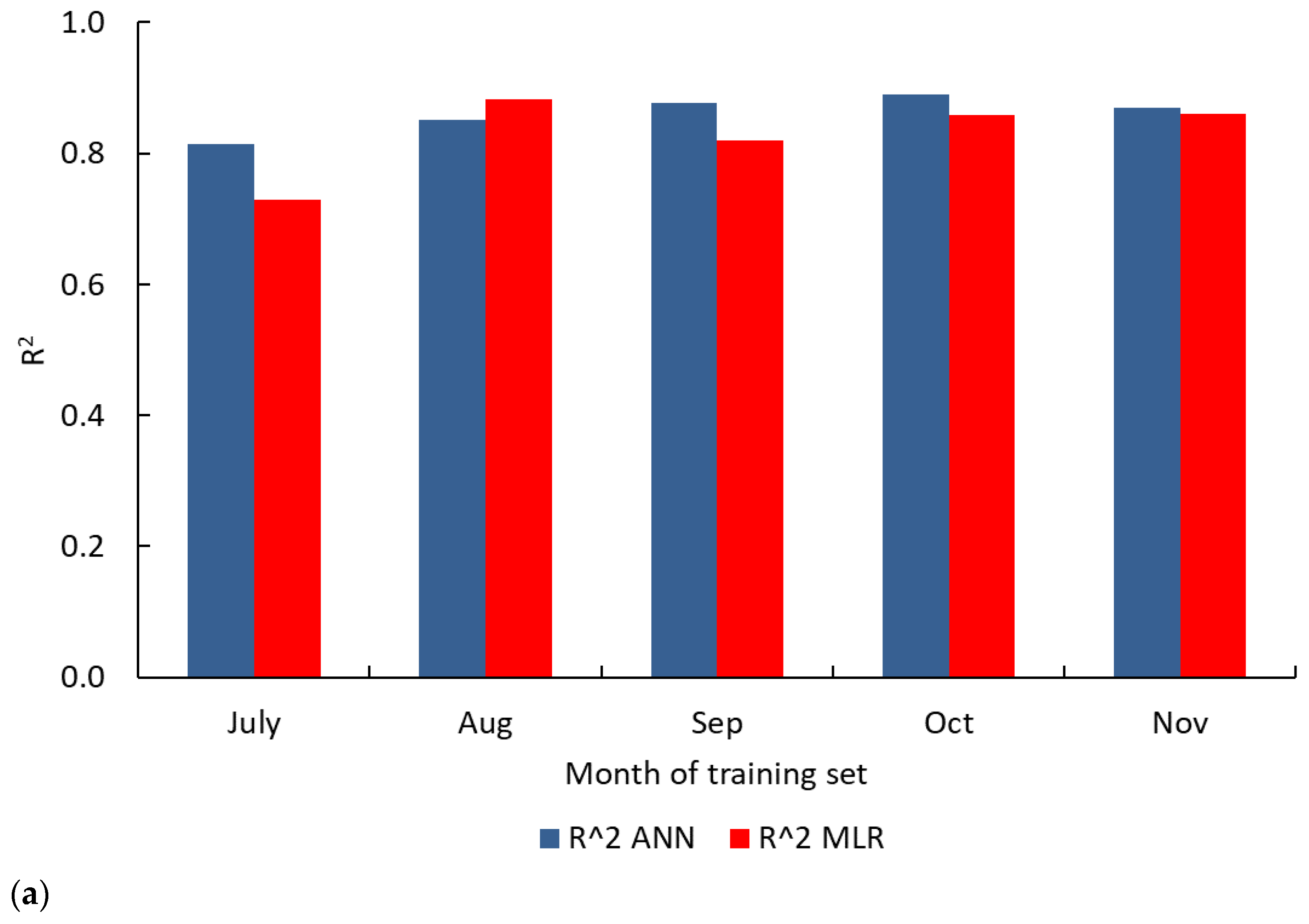
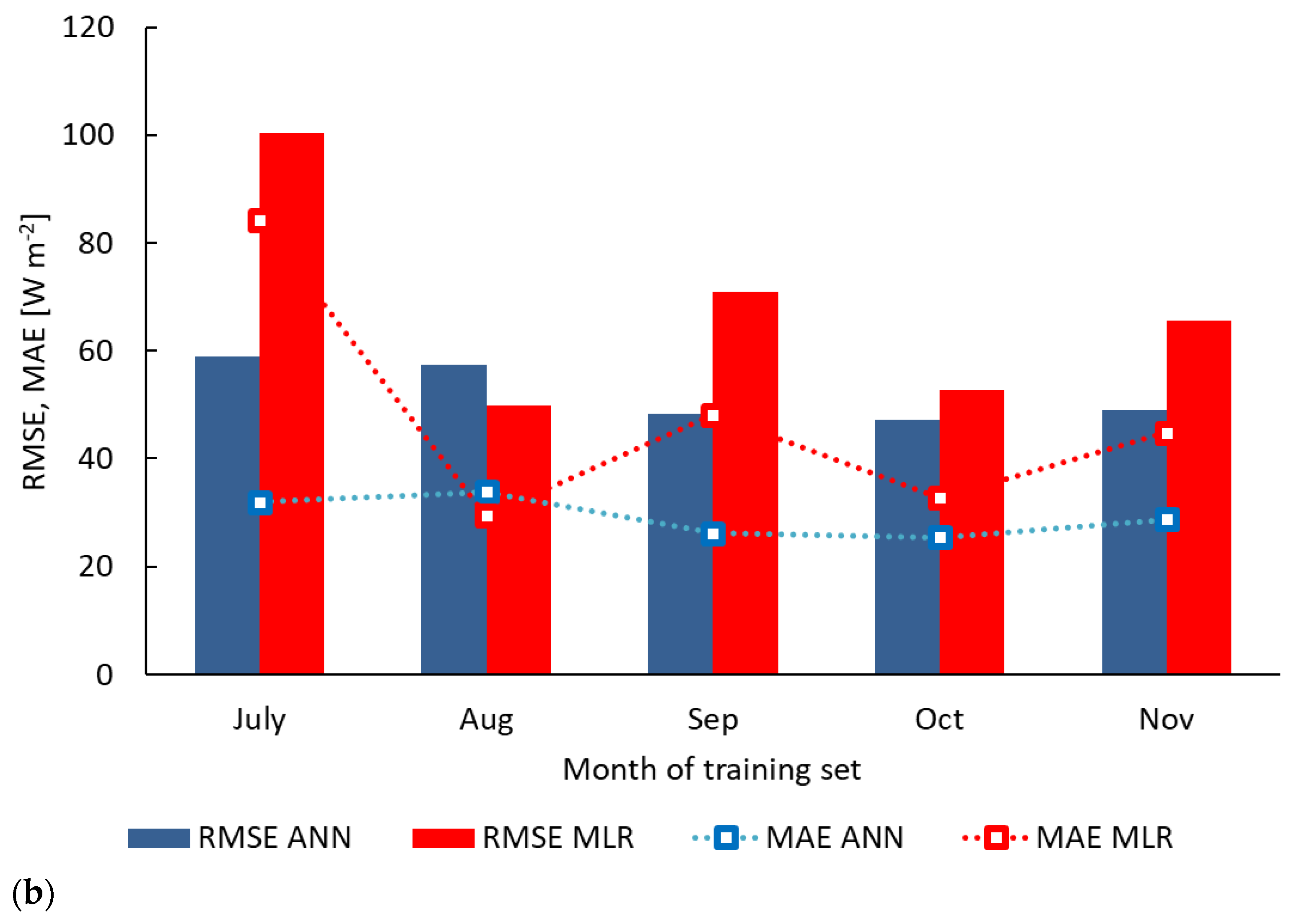
Training ANN evapotranspiration models requires data acquisition of field measurements using complex and expensive methods, e.g., the eddy covariance system [37]. Hence, from a practical point of view, it is of interest to examine the model performance with short training periods. In this study, model performance was examined with one-month and one-week training periods. Running the models using a one-month training period in 2017 showed that ANN was superior to MLR (Figure 3) except when August data was used for training, where MLR performed better than ANN. Specifically, training the ANN model using October data provided the highest R² = 0.89 (only slightly lower than 0.92 obtained with the whole data set) and lowest values of RMSE and MAE, 47.3 and 25.4 W m⁻² respectively. On the other hand, training the ANN model using July 2017 data provided the lowest R² = 0.81.

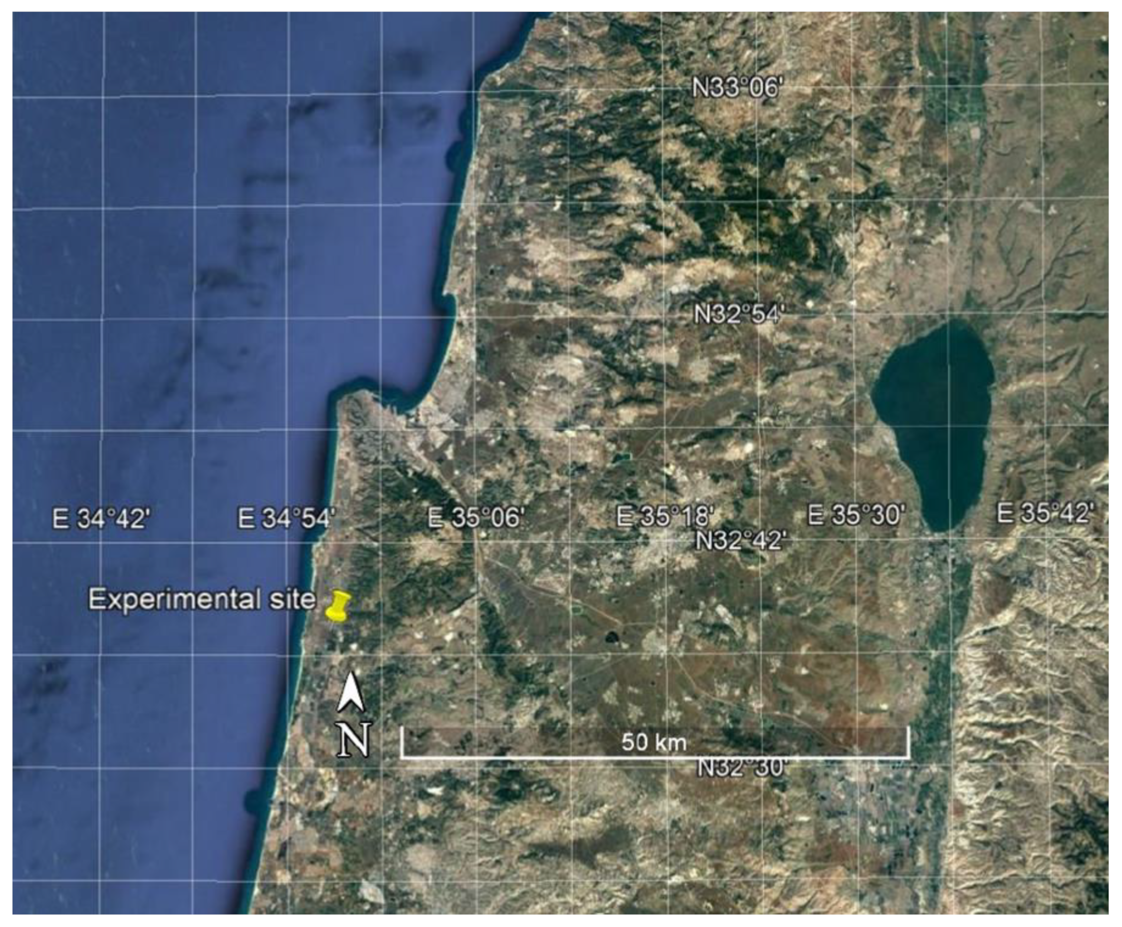
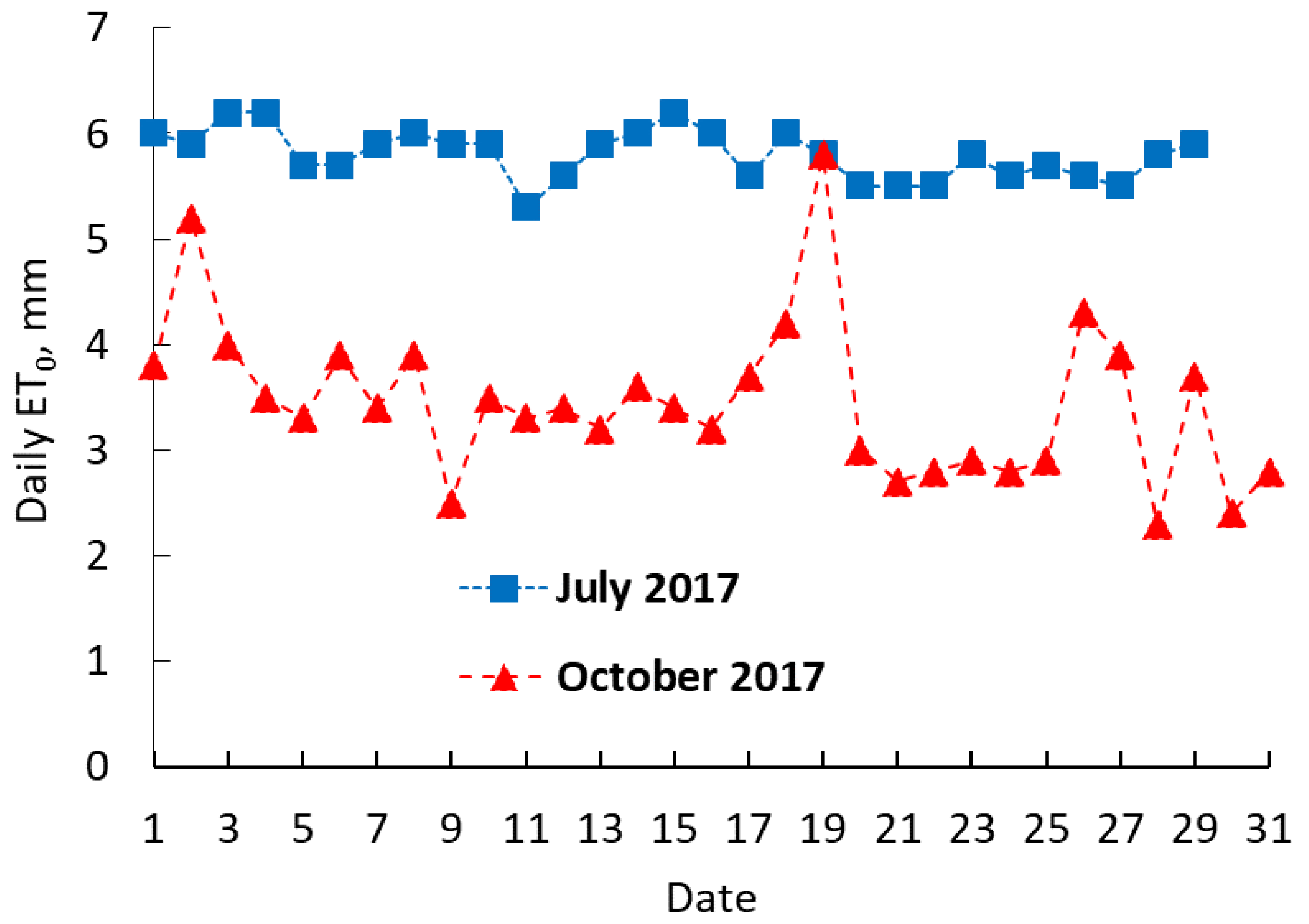
A possible reason for this difference is that at the experimental site, weather conditions are much more variable during October than during July, which provided a training dataset for a more reliable model. To illustrate this difference, we analysed the reference evapotranspiration, ET₀, from a nearby meteorological station operated by the IMS—Israel Meteorological Service—during October and July 2017. We chose ET₀ for this comparison because it represents an integrated measure of weather conditions. The results of this analysis are presented in Figure 9. The results show a much larger variability of weather conditions in October than in July, which supports the improved performance of the model when trained using October rather than July data.

The MLR model performance was best when trained using August 2017 data (Figure 3); which gave R² = 0.88, RMSE = 49.9 W m⁻² and MAE = 29.4 W m⁻². August weather in Israel is rather monotonous without much variability, which implies that such conditions are advantageous for the MLR model. This result is different from the ANN model, where variable weather conditions during October were presumably favourable. This difference between the two methods requires further research.

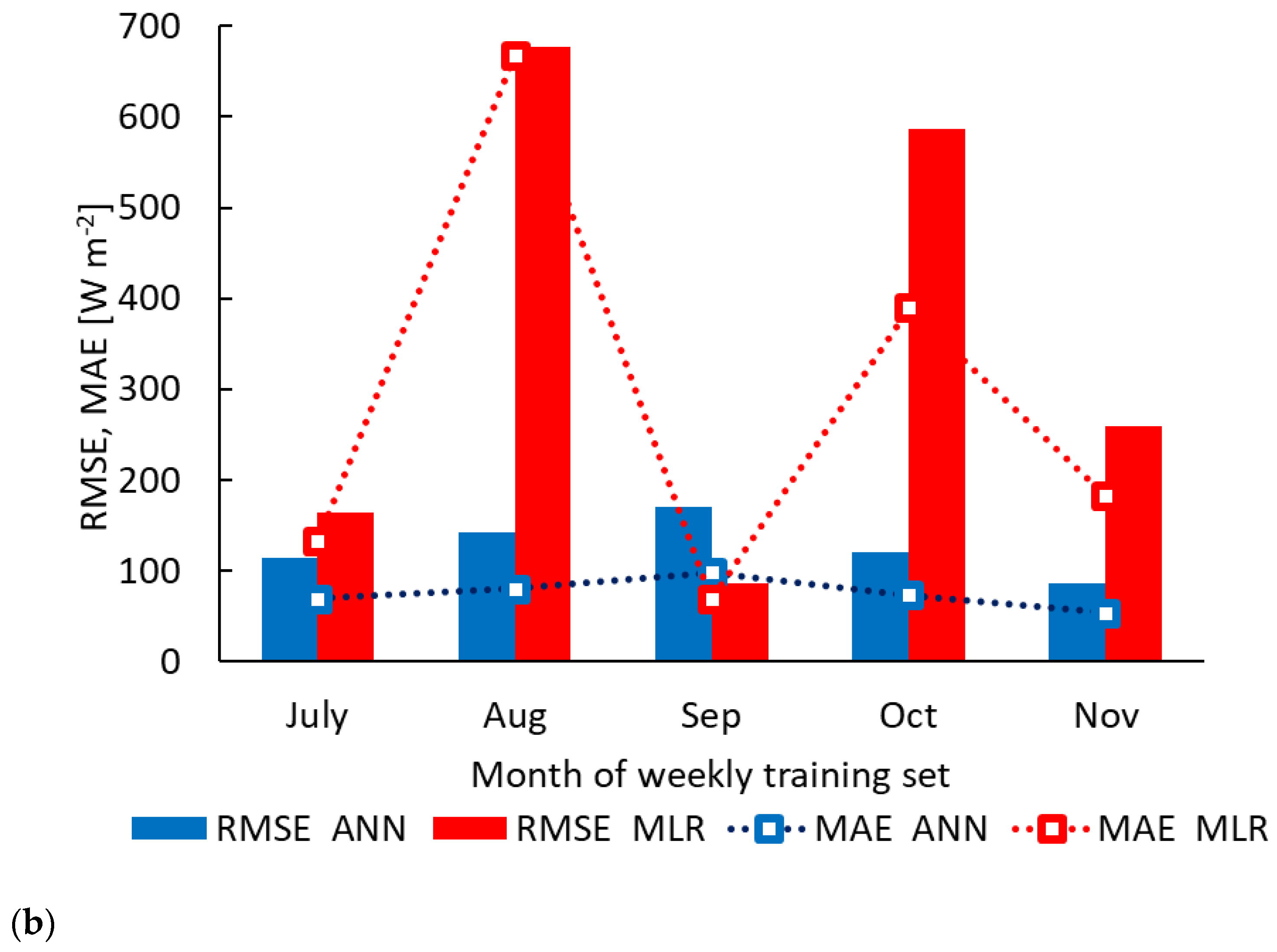
Analysis was also performed using a one-week training period. The results in Figure 4 showed that when the one-week training period used September, October, and November data, the ANN model’s performance (R²) was higher than during July and August. Again, this can be explained by the diverse weather during the autumn months (September, October and November) compared to the uniform weather during the summer months of July and August. Regarding the MLR model, R² with training during a week in October and November was lower than during July, August, and September. Similar to the results for one-month training, this result of the MLR model is opposite to that obtained with the ANN model and deserves further research.

The ability of the ANN model to provide satisfactory R² with one-week training in certain months is in agreement with Kelley and Pardyjak [10], who showed high performance of an ANN model that was trained during seven days under open field conditions. Kelley and Pardyjak [10] also highlighted that robust estimation could be obtained, provided climatic and field conditions of the seven-day training period were similar to those during data validation.

A comparison between the results obtained with one month (Figure 3) and one week (Figure 4) training shows that using data of September, October, and November, R² of the ANN model is approximately the same for the two training periods, weekly and monthly. However, the RMSE and MAE of the ANN model trained with a one-month data set are significantly lower (indicating better performance) than those of the ANN model trained with a one-week data set. The ANN model trained during one month generated a much higher R² than the model trained during one week using July and August data. For the MLR model, training using one-month data yielded higher R² and lower RMSE and MAE than training using one-week data, regardless of the month or week chosen for training.

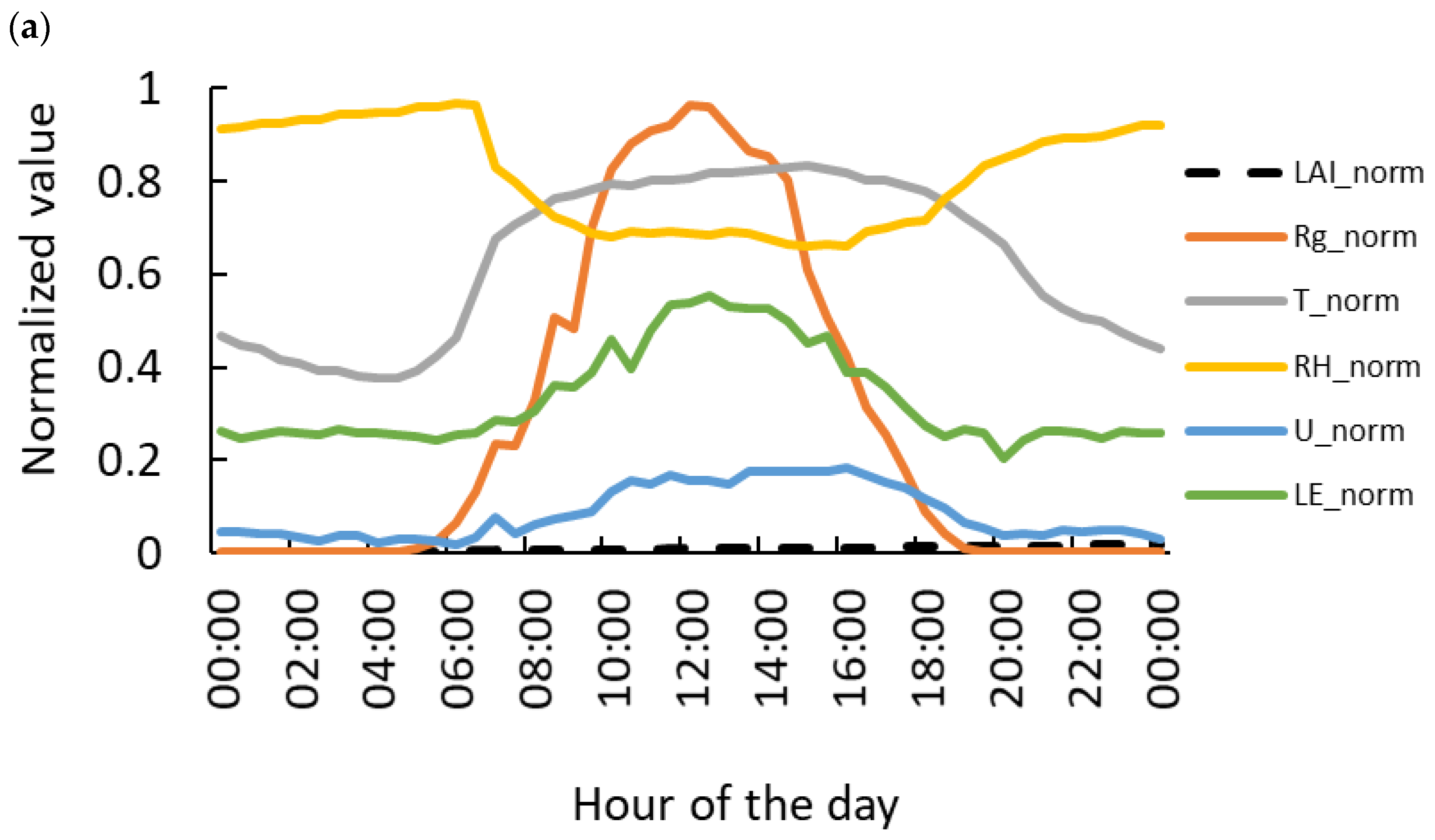
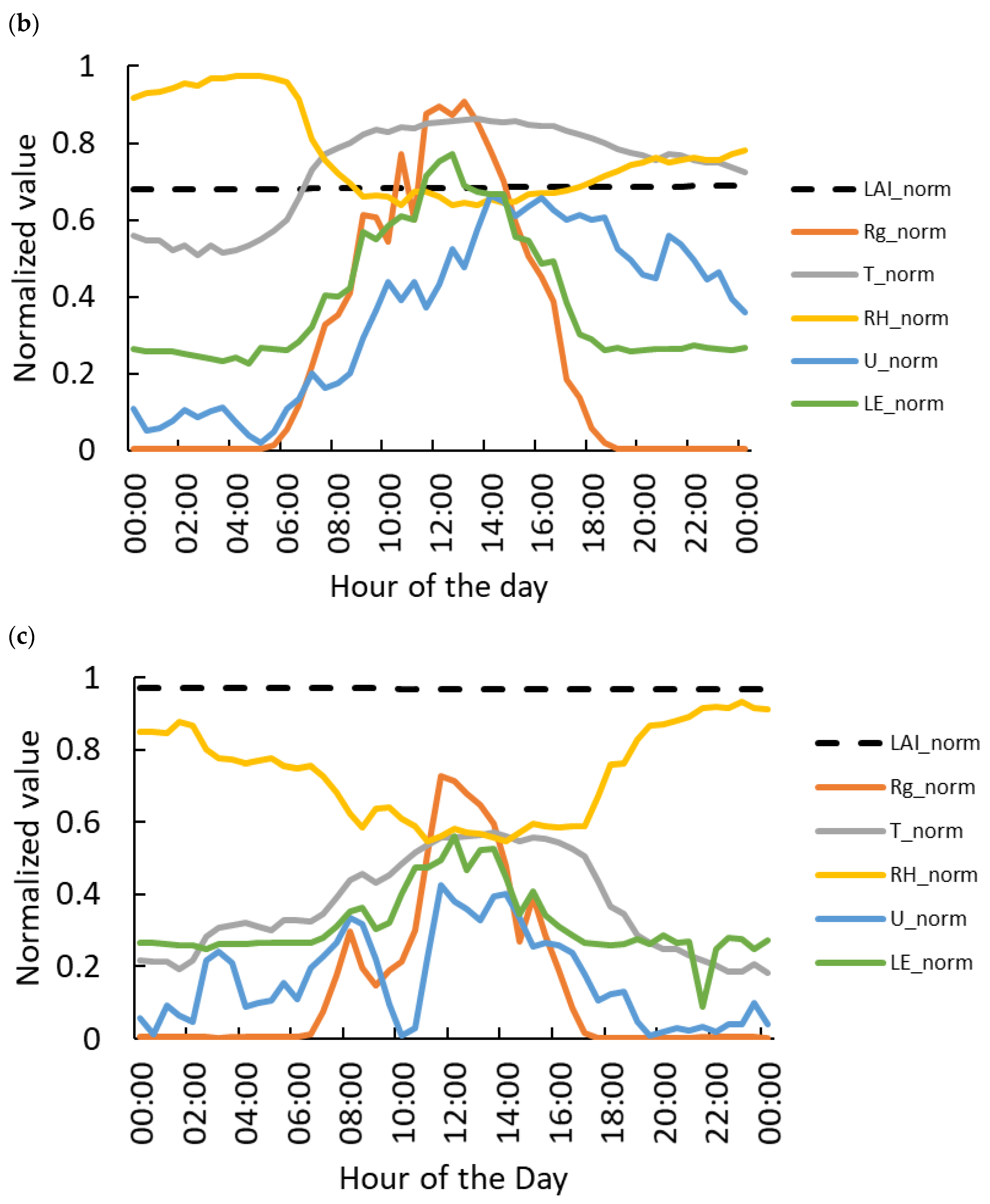
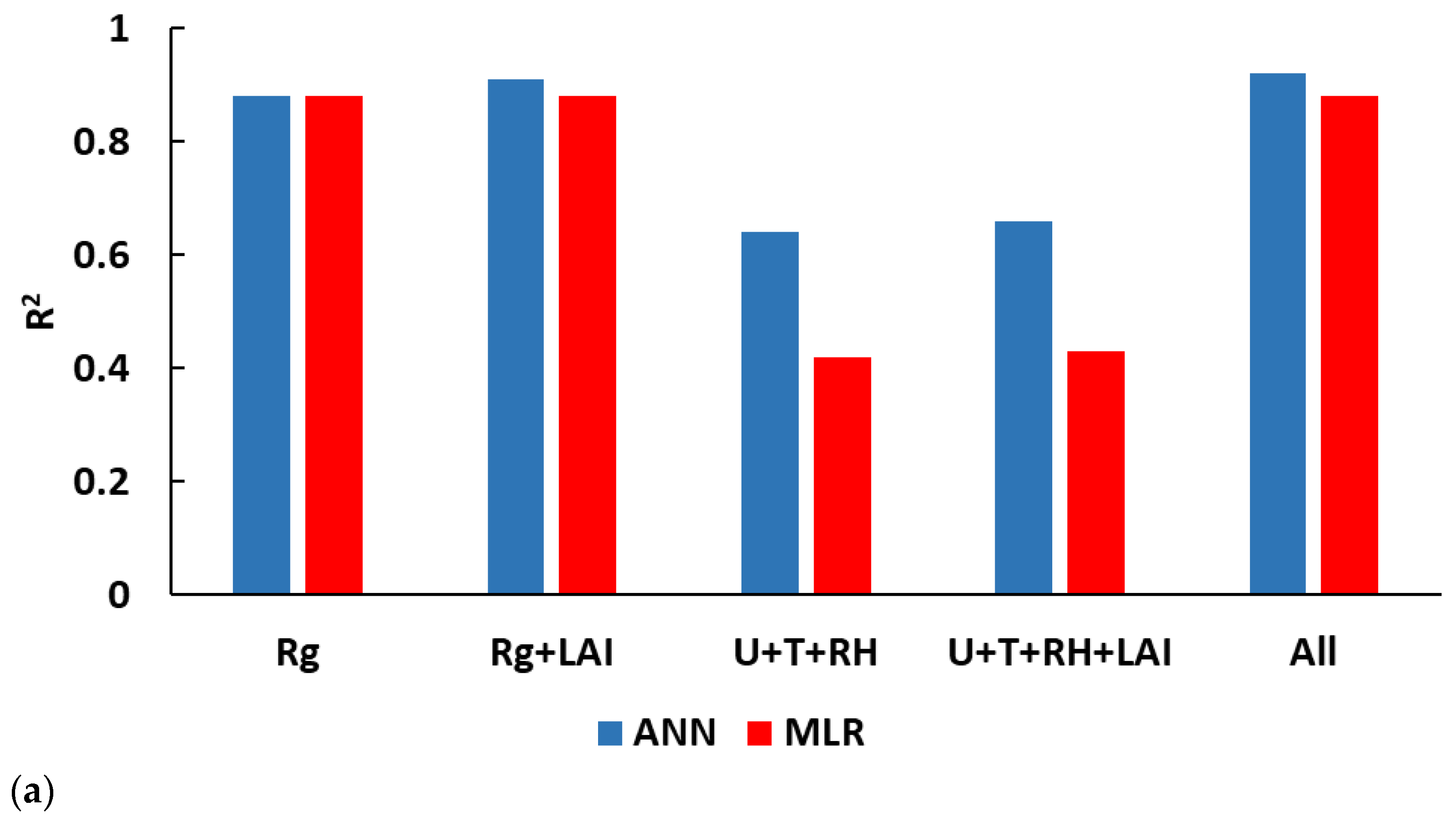
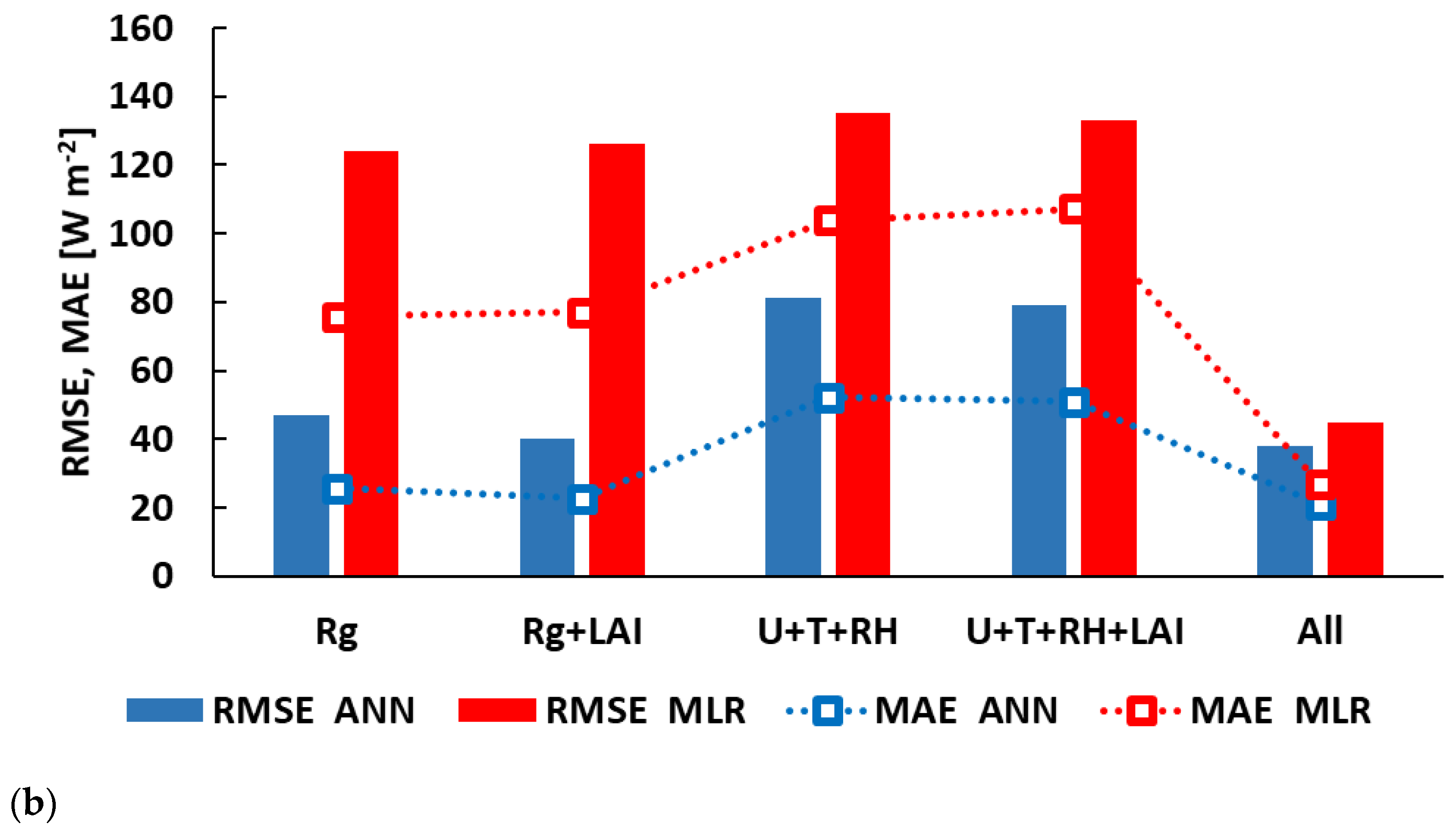
Analysis showed that the input variable most influential on evapotranspiration was solar radiation, then wind speed, air temperature, and air relative humidity. The strong influence of solar radiation on LE in screenhouses is mainly due to the decoupled microclimate [35] in this environment, as demonstrated by Möller et al. [16] for a pepper screenhouse, by Haijun et al. [17] for a banana screenhouse, and by Hadad et al. [24] for pepper screenhouses and greenhouses. In such protected environments, the low wind speed enhances the contribution of radiation to evapotranspiration. This result is also in general agreement with Zanetti et al. [4], who estimated reference evapotranspiration using ANN models under open field conditions, and showed that solar radiation and minimum/maximum air temperature data are sufficient to derive reliable estimates of ET₀.

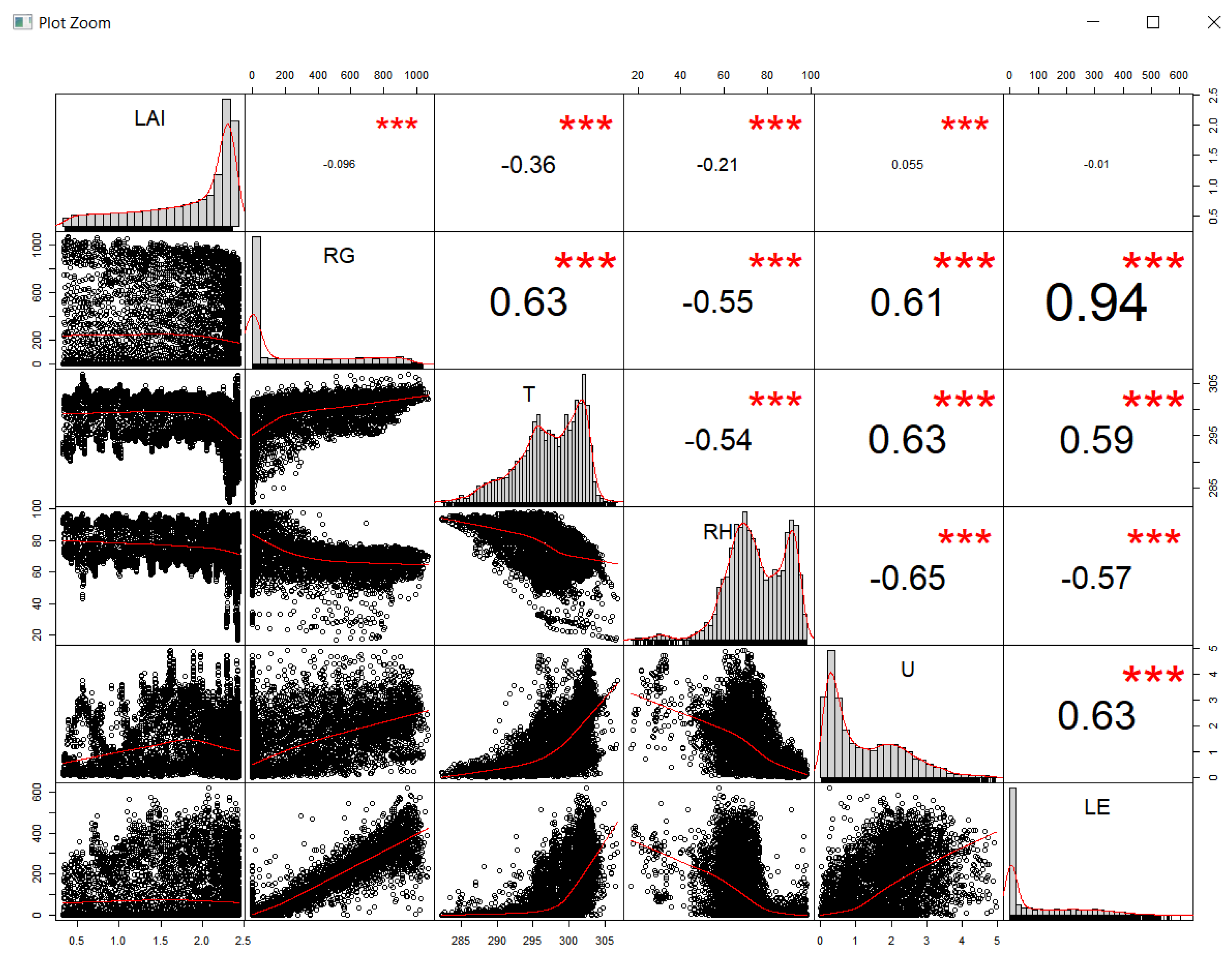
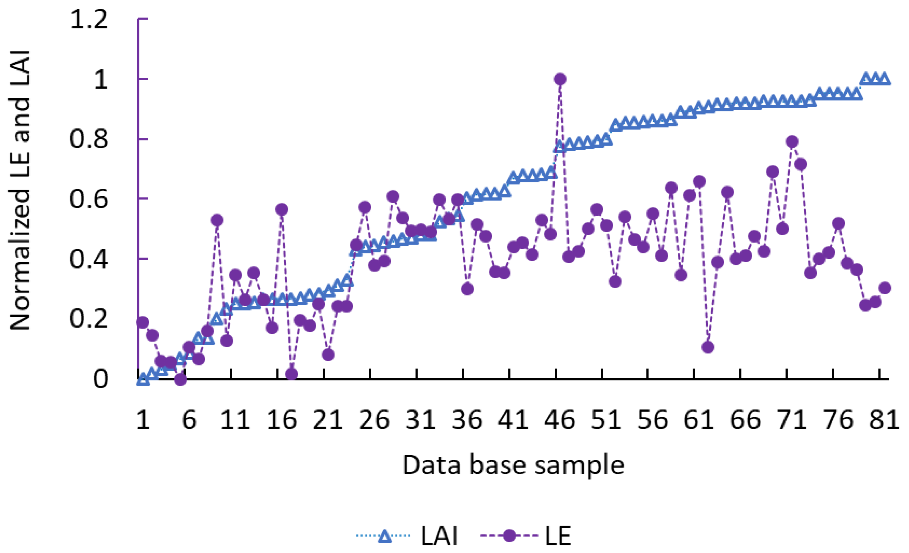
The influence of LAI on LE depended on the time scale of the analysis. When analysing the half-hourly values, the addition of LAI only made a minute improvement on the models’ performance (Figure 6a,b). The small contribution of LAI to model performance was due to its low correlation with LE on the half-hourly timescale (Figure 5). However, when data were analysed on a daily timescale (Section 3.6.3), the addition of LAI to the input data set increased R² of the ANN and MLR models by 31% and 18%, respectively.

Comparing the performance of the ANN model with the commonly used Penman-Monteith model over the whole data of 2017 showed that the ANN is superior to PM. This result is in general agreement with the literature, where other versions of ANN were evaluated compared to the PM model. For example, Odhiambo et al. [5] showed that a model which combined neural networks and fuzzy logic was in better agreement with measurements than PM-FAO56. Manikumari et al. [6] used the deep learning neural network (DLNN) methodology to estimate ET₀ in a region of rice cultivation in India. Results of this study also showed superior performance of the DLNN model over the PM-FAO56. Zanetti et al. [4] demonstrated the ability of the ANN model to estimate ET₀ with reasonable accuracy. These literature reports studied LE or ET₀ in open fields, whereas our study investigated a screenhouse crop. The superiority of the different versions of the ANN model over PM, in both the open field and protected environments, is probably due to its high flexibility in describing the complex and non-linear interactions between meteorological variables and evapotranspiration. On the other hand, it should be noted that the ANN approach is totally empirical as compared to the PM model; the latter is based on physical principles, and thus may provide more insight into the mechanism of the evapotranspiration process.

Several issues that were not considered in this research require further study. The first, related to the data set, is sensor height relative to screenhouse height and its effect on the models. Although the measurement system was positioned at different heights during each campaign (Table 1), all data were aggregated into a single database. It is possible that separately considering data from different heights would improve model performance. On the other hand, machine learning approaches require large amounts of data for reliable performance, and deriving a distinct model for each sensor height would cause the models to be based on small pieces of data. For this reason, in the present study, data from all sensor heights were collected into a single large data set.

Secondly, developing models using short training periods is essential from a practical point of view. Installing measurement systems such as those in the present study, including the eddy covariance system, is highly time-, cost-, and labor-consuming. The current analysis considered training periods as short as a month or a week. The results showed that training during specific seasons of the year was advantageous over other seasons. In a future study, collection of a more extensive data set would enable a more detailed analysis to better identify the optimal season for training with a short-term data set.

5. Main Conclusions

This study examined the performance of artificial neural network and multiple linear regression models in estimating the actual evapotranspiration of banana screenhouses. In most cases, ANN was superior to MLR. Models could be trained using a relatively short period dataset of one month and still perform reliably. When training used a weekly dataset, the performance of the MLR model was generally poor; however, the ANN model’s performance was reliable when the weekly dataset was from a season that included diverse weather conditions. Analysis with limited meteorological data showed that when the model was trained with solar radiation only, results only slightly declined relative to the analysis using all variables. Adding the leaf area index as an input variable to the solar radiation somewhat improved the models’ performance. When trained over one season and applied on a similar banana screenhouse during another season, the performance of the ANN model was satisfactory (R² = 0.94) and superior to the MLR model. Comparing the machine learning models with the Penman-Monteith model for screenhouse banana plants, the PM performance was somewhat lower than the ANN model and approximately similar to the MLR model.