
Household Water Consumption in Spain: Disparities between Region


1
Department of Economic Analysis, University of Zaragoza, 50005 Zaragoza, Spain
2
Department of Applied Economics, University of Zaragoza, 50005 Zaragoza, Spain
*
Author to whom correspondence should be addressed.
Water 2022, 14(7), 1121; https://doi.org/10.3390/w14071121
Submission received: 8 February 2022
/
Revised: 20 March 2022
/
Accepted: 28 March 2022
/
Published: 31 March 2022
(This article belongs to the Section Urban Water Management)
Abstract
:This paper studies the regional consumption of household water in Spain in the period 2000–2018. The use of the methodology proposed by Phillips and Sul allows us to conclude that there is no single pattern of behavior across the Spanish regions. By contrast, we can determine the existence of three convergence clubs, confirming serious regional disparities in water consumption. Navarra, País Vasco, La Rioja, and Cataluña are included in the convergence club that shows the lowest levels of household water consumption, while the Islas Canarias, Comunidad Valenciana, Castilla y León and Cantabria belong to that with the highest consumption. The determinants of the forces that drive these convergence clubs are difficult to identify because the demographic, economic and structural variables of the network interact in different ways. Nevertheless, we can select a group of explanatory variables that help to explain the formation of the convergence clubs. These are regional household income, the birth rate in the regions, and the regional spending on environmental protection. Increments in the levels of these variables are helpful for reducing household water consumption.
1. Introduction
Water has been identified not only as one of the most important natural resources for human life but has also been shown to be a source of prosperity and wealth, as Arbués, et al. [1] note. In addition, as Marshall [2] points out, it is well known that water has played a crucial role in the location, function, and growth of communities. Water and humanity have been, are, and will be inextricably linked. As a consequence, the scarcity of this natural resource represents a serious danger to life and prosperity, and governments throughout the world need to invest large sums of human and technological resources to ensure adequate water supplies.
Whilst water scarcity is commonly associated with less developed countries (Africa in particular), this is a problem that also affects other regions, even in the heart of Europe. This is explained by the fact that water availability and use are unevenly distributed, despite the relative abundance of freshwater resources in certain European regions. These disparities are especially worrying if the results and warnings of the European Environment Agency (EEA) are taken into account. This organization has estimated that the demand for water in Europe has increased over the last 50 years, involving an overall decline in renewable water resources of 24% (in per capita terms) with the subsequent increase in hydric stress in European regions.
The consequence of this increase in demand is that about one third of the European Union (EU) territory is exposed to water stress conditions, either permanently or temporarily. Furthermore, it is important to note that this problem does not only affect Southern European countries, such as Greece, Portugal, and Spain. Rather, this is also becoming a problem in Northern regions, including parts of the UK and Germany. This dark panorama becomes even darker if we take into account the threats of climate change, which increasingly conditions human life.
To mitigate this water scarcity problem, the EU has launched a plethora of environmental policies with the general aim of significantly reducing the negative effects of pollution, over-abstraction and other pressures on water, and ensuring that a sufficient quantity of good quality water is available. However, although the need to achieve these targets is beyond question, the main goal and the greatest challenge of the EU agenda is to increase the efficiency of water management, especially by reducing water consumption. We should note that the different policies aimed at meeting this target have important economic implications, as analyzed in Hutton and Varughese [3].
The need to find methods of increasing water use efficiency is a clear invitation to governments to assess and rethink the way in which this resource has been exploited in recent years. In this scenario, water must be conceived of as a basic resource for survival and be managed strategically as a scarce economic good of growing value, without losing sight of the human rights approach that its use and enjoyment entails. The challenge for local governments is to ensure water sustainability by implementing strategies in the short and medium term to reduce the potential for water stress in the coming years. This leads us to consider that we should begin to manage new policies for change in the understanding, use, dimension, valuation, and projection of this limited but indispensable resource not only for life, but also for global economic growth. It is not for nothing that having access to clean water and sanitation is the sixth Sustainable Development Goal (SDG) of the 2030 agenda (United Nations World Water Development Report [4]), which includes explicit targets regarding the improvement of water quality worldwide and the increase in water use efficiency and reduction in water scarcity, as studied in Ho, et al. [5] or in Hoekstra, et al. [6]. Following these authors, this objective is divided into six targets. The first two targets aim to achieve universal and equitable access to safe and affordable drinking water for all. The third target is to improve water quality by reducing pollution. Number four seeks to substantially increase water use efficiency in all sectors and ensure sustainability and freshwater supply to address water scarcity and substantially reduce the number of people suffering from such scarcity. Finally, the last two targets aim to implement, protect, and restore water-related ecosystems and integrated water resources management at all levels, including through transboundary cooperation. Therefore, governments should adopt the appropriate polices to achieve these goals.
While these policies are being developed and taking effect, the situation remains very worrying, especially in Southern European countries. The Spanish case is probably one of the most outstanding examples. This can be better understood if we take into account the results of Hofste, et al. [7] who classify Spain in the group of “high baseline water stress” countries, being the 28th country with the highest water stress (the 5th European country after Cyprus, Andorra, Belgium, and Greece). The analysis of these water problems has attracted the interest of several researchers, who have studied the evolution of Spanish water consumption from different perspectives. Although the volume of the related literature is substantial, we would highlight the papers by Cazcarro, et al. [8], Estrela, et al. [9] and Gracia-De-Rentería, et al. [10] from a general perspective, and the papers by Martínez-Espiñeira [11], Arbués, et al. [12], Hoyos, et al. [13], and Sauri [14] from the perspective of urban water consumption. We are aware of the existence of a huge volume of literature on water consumption which is not focused on the Spanish case. Appendix A provides a short summary. Besides, we would also note the recent reviews by Fuentes, et al. [15], Bich-Ngoc and Teller [16] and Abu-Bakar, et al. [17]. These papers reveal the problem of water scarcity in different parts of Spain, a problem recently aggravated by the severe drought suffered in 2005–2009 and by the consequences of the Great Recession.
This dark scenario has led Spanish governments to react and implement policy, management, administrative and infrastructure measures aimed at the progressive and continuous reduction in water consumption. The consequence is that household consumption noticeably decreased from 168 lid (liters per inhabitant per day) in 2000 to 133 lid in 2018. However, we cannot consider that the effectiveness of these measures has been similar across all the Spanish regions. Serious differences seem to persist, with the negative consequences that this could entail for an effective coordination of a common water policy throughout the Spanish territory.
Against this background, the aim of this paper is to determine whether there is a common pattern of behavior in household water consumption in all Spanish regions or, by contrast, whether regional water consumption disparities are so important that several patterns of behavior can be found. To do so, we can apply the statistics proposed in Phillips and Sul [18,19] to test the null hypothesis of convergence for a set of data. If we are not able to reject this hypothesis, we can conclude in favor of the existence of a common behavior among all Spanish regions in terms of water consumption and the disparities would not be statistically significant. However, if we are able to reject it, then we will be able to identify multiple patterns of behavior and, consequently, determine the number of estimated convergence clubs, the regions associated with them, and the forces that may drive them. The use of these techniques allows us to consider the dynamics of the variables under analysis. This is a relevant point, given that most of the previous literature is based on the use of cross-sectional data and, consequently, cannot capture the dynamic and trend components.
The remainder of the paper is organized as follows. Section 2 describes the data, methodology and analytical framework. Section 3 presents the empirical results of the convergence analyses and a description of the convergence clubs. Finally, Section 4 draws the most important conclusions and identifies the economic implications and policy recommendations.
2. Data and Methods
2.1. Database
Household water consumption has been measured by the volume of water registered according to data supplied by households. These data are collected by the Spanish Institute of Statistics (INE) and are annually available for the period 2000–2014. Since this year, they have been published biennially (2016 and 2018). Then, we have linearly interpolated the data of 2017 to compile a complete data set for the 2000–2018 period. The data are measured in liters per inhabitant per day (lid) and we include information of the total Spanish household water consumption and those of the 17 Spanish regions. To better understand the evolution of this variable, some descriptive statistics are presented in Table 1.
As can be seen in this table, household water consumption in Spain at the beginning of the sample was 168 lid, whilst the value at the end of the sample was lower (133 lid), which implies a total reduction of nearly 21%. This reduction may have occurred as a consequence of a number of factors and it is not easy to identify which has been the most important one. In our view, this reduction has been the result of a combination of the appropriate measures taken during recent years and the effect of some unexpected events, such as the Great Recession or the drought periods. Tortajada, et al. [20] and Sauri [14] offer very useful insights to better understand why the household water consumption has reduced in Spanish regions. We should also note that, at the end of the sample, the regions with the highest household water consumption were Comunidad Valenciana (175 lid) and, quite surprisingly due to the fact that it has a (comparatively) very wet climate, Cantabria (172 lid). By contrast, those with the lowest levels of water consumption were País Vasco (104 lid), Navarra (114 lid), and La Rioja (116 lid), the three located in the north of the country and experiencing a (comparatively) wet climate.
If we analyze the annual average growth rates, we observe that Spanish household water consumption decreased following a −1.3% annual average growth rate during 2000–2018, which is an excellent result if we interpret it in terms of sustainability. However, this decreasing pattern of behavior is far from being homogeneous across the Spanish regions. For instance, the values of the regional growth rates go from −2.4% (La Rioja) to 0.3% (Murcia and Comunidad Valenciana), with these two last regions increasing the household water consumption for the total sample.
This disparity also appears if we split the total sample into the three different time periods included in the Table: 2000–2008, 2008–2013 and 2013–2018. This segmentation of the sample could help us to analyze whether the recent economic crisis, commonly referred to as the Great Recession, led to a change in household water consumption patterns. The first segment is clearly related to the pre-Great Recession period, whilst the next two segments are associated with the difficult period of the crisis and the subsequent recovery period, respectively. We can observe that the average annual growth rate in Spain remained unaltered if we only consider the pre-Great Recession (2000–2008), but it clearly varied as a consequence of the Great Recession, with a very significant fall at the beginning (−3.0 during 2008–2013), followed by a moderate increase (0.5 during 2013–2018).
This aggregated behavior for Spain as a whole clearly hides the above-mentioned heterogeneity of the regions. For instance, if we consider the 2000–2008 period, the average annual growth rates go from −3.8% (Cataluña) to 1.8% (Asturias), with another five regions showing positive growth rates. During the next period, 2008–2013, the rates vary from −7.0% (Asturias) to 0.9% (Castilla y León). We should note that most of the regions had negative growth rates during this period, with the exceptions of Castilla y León and Islas Baleares. Finally, the final segment (2013–2018) is the most heterogenous. The values of the growth rates go from −3.3% (País Vasco) to 3.7% (Murcia), with 10 regions increasing their household water consumption.
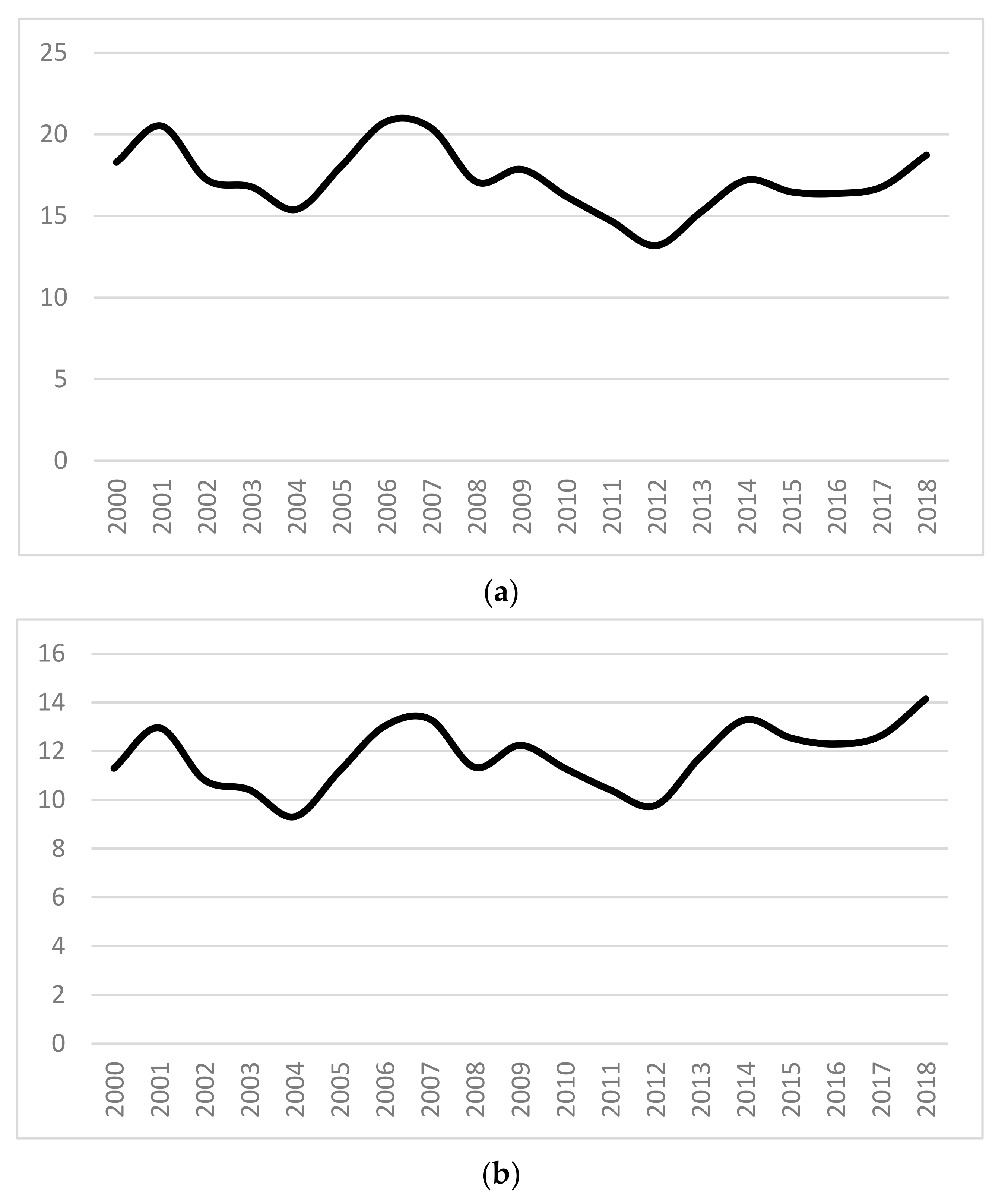
The most important insight emerging from this initial descriptive analysis is the existence of considerable disparity between household water consumption in the Spanish regions. This is even more apparent if we analyze the evolution of two dispersion measures: the standard deviation and the coefficient of variations. Figure 1a,b present the values of these two statistics. As we can see, both statistics show a decreasing path up to 2012, whilst they increase after this period. This confirms our initial suspicion of the heterogeneity of Spanish regional household water consumption. Both figures point to the presence of divergent behavior in the sample, if we interpret them in σ-convergence terms. However, the methods used do not seem the most appropriate to test for convergence and, consequently, for determining the existence of a common pattern of behavior across the Spanish regions. The next section is devoted to describing the methodology we use to discern whether the regions behave differently or, by contrast, show a common pattern of behavior.
Figure 1a,b present the evolution of the cross-sectional standard deviation and the cross-sectional coefficient of variation of the sample.
2.2. Convergence and Phillips-Sul Methodology
As we have previously seen, the pattern of behavior of household water consumption does not appear to be similar across the Spanish regions. Rather, the σ-convergence analysis suggests the existence of a divergent behavior. Given that the method employed in the previous Section is based only on a visual inspection of the evolution of the cross-sectional dispersion, it seems appropriate to use some econometric methods that allow us to explicitly test for convergence.
In this regard, we should note that the concept of convergence has been defined in the economic literature as a process where the dispersion of a variable, usually per capita Gross Domestic Product (GDP), reduces for a group of countries or regions. The interest in this type of analysis grew due to the seminal paper by Barro and Sala-i-Martí [21] who define the standard concepts of β- and σ-convergence. These initial tools were subsequently substituted by more sophisticated analysis, based on the concept of stochastic convergence, based on the results of Carlino and Mills [22] and Bernard and Durlauf [23], who base their results on the use of unit root tests.
However, none of these papers develop or use a statistic that focuses on testing the null hypothesis of convergence. This problem is considered in Phillips and Sul [18], PS hereafter, who designed a statistic that explicitly tests for convergence. This statistic has become popular nowadays and we can find several examples of its use for analyzing the disparities in the evolution of variables for a number of countries or regions. We can cite the papers by González-Álvarez, et al. [24], who analyze the evolution of obesity for a sample of countries; Clemente, et al. [25], who study the dispersion of health expenditure across the US states; Rodríguez-Benavides, et al. [26], who investigate convergence in Latin America; and Jangam, et al. [27], who focus on electricity consumption in India.
In spite of the interest in this methodology, we should note that its application to environmental variables is relatively scarce. However, we can cite some papers where convergence has been analyzed for this type of variable. Most of them are devoted to the analysis of carbon dioxide emissions: Camarero, et al. [28], Parker and Bhatti [29] and Payne and Apergis [30,31], amongst others. Similarly, Camarero, et al. [32] study eco-efficiency, whilst Alcay, et al. [33] analyze the case of municipal solid waste generation in Spain.
By contrast, the case of water consumption has not received much attention in the literature, at least so far as convergence analysis is concerned. We have only found the paper by Tzeremes and Tzeremes [34], who use the PS methodology to study the evolution of water prices in the US states. There are also a few papers that analyze convergence without using the PS methodology. For instance, Portnov and Meir [35] study convergence in urban water consumption in Israel, and Acuña, et al. [36] analyze the case of Chilean residential water consumption. Instead of using the methodology proposed by PS, their results are based on the use of the β- and σ-convergence notions and, therefore, are not free from the criticism made by Quah [37] of these tools. It therefore seems appropriate to use the PS methodology for the analysis of household water consumption across Spanish regions.
Following PS, let us consider that Xit represents the log of our variable of interest, namely the household consumption of water in the Spanish regions, with i = 1, 2,…, 17 (the 17 Spanish regions) and t = 2000,…, 2018. This variable can be decomposed as Xit = δit μt, where μt and δit are the common and the idiosyncratic components, respectively. PS suggest testing for convergence by analyzing whether δit converges towards δ. To do so, they first define the relative transition component:
In the presence of convergence, hit should converge towards unity, while its cross-sectional variation, Hit, is defined as follows:
and should go to 0 when T goes towards infinity. Then, PS test for convergence by estimating the following equation:
where , and r = 0.3. Equation (3) is commonly known as the log-t regression. The null hypothesis of convergence is rejected whenever parameter β is lower than 0. PS suggest estimating model (3) by methods that correct for the presence of autocorrelation and heteroscedasticity and, later, employ the t-statistic to test the null hypothesis β = 0. The use of these robust methods ensures that this t-ratio converges towards a standard N(0,1) distribution and, therefore, we will reject the null hypothesis of convergence whenever this t-statistic takes values lower than −1.65.
If we reject convergence, PS propose a robust clustering algorithm for identifying convergence clubs in a panel, which operates as detailed in Appendix B. PS recommend performing convergence club merging tests after running the algorithm using Equation (3) in order to avoid an over-estimation of the number of convergence clubs. Finally, we should note that we have followed the suggestion of PS and extracted the trend components of the series by filtering them using the Hodrick and Prescott [38] filter, applying the standard value λ = 400.
3. Results and Discussion
3.1. Results
The results of the use of the PS statistic are presented in Table 2. As we can see in Panel I, the log-t ratio takes the value −27.54 and clearly rejects the null hypothesis of convergence. This implies that household water consumption does not follow a common pattern of behavior across the Spanish regions, confirming the heterogeneity observed in the descriptive analysis. However, it is possible that some regions may exhibit similar behavior and create the existence of convergence clubs. In order to analyze this, we have applied the clustering algorithm proposed by Phillips and Sul [18]. The results, which are reported in Panel II of Table 2, allow us to estimate the existence of three convergence clubs. Then, we should conclude that Spanish regional household water consumption shows important differences across regions.
The analysis of the composition of the estimated convergence clubs allows us to gain some interesting insights. To make the interpretation of the results easier, Figure 2 shows the geographical composition of each estimated convergence club on a map of Spain. Using this figure, we can see that Club 3 show the lowest consumption and includes northern and north-eastern regions (País Vasco, Navarra, La Rioja and Cataluña). Club 2 includes some regions located in the center and in the south of Spain (Andalucía, Extremadura, Murcia, Castilla la Mancha, Madrid and Aragón) and, additionally, Galicia (north) and the Islas Baleares (Mediterranean Sea). The most scattered group is Club 1, which is formed by Cantabria, Castilla y León, Comunidad Valenciana and the Islas Canarias. This Club 1 shows the highest household water consumption. The inclusion of Cantabria, a northern region with a wet climate, in this group is noteworthy. However, the relatively high level of household water consumption in this region is well known, arguably related with metering procedures. Consequently, it would be necessary for the regional authorities to make a greater effort to invest in the supply network, while requesting municipalities that have not yet installed meters to proceed with their installation as the lack of meters is a possible cause of this higher consumption.
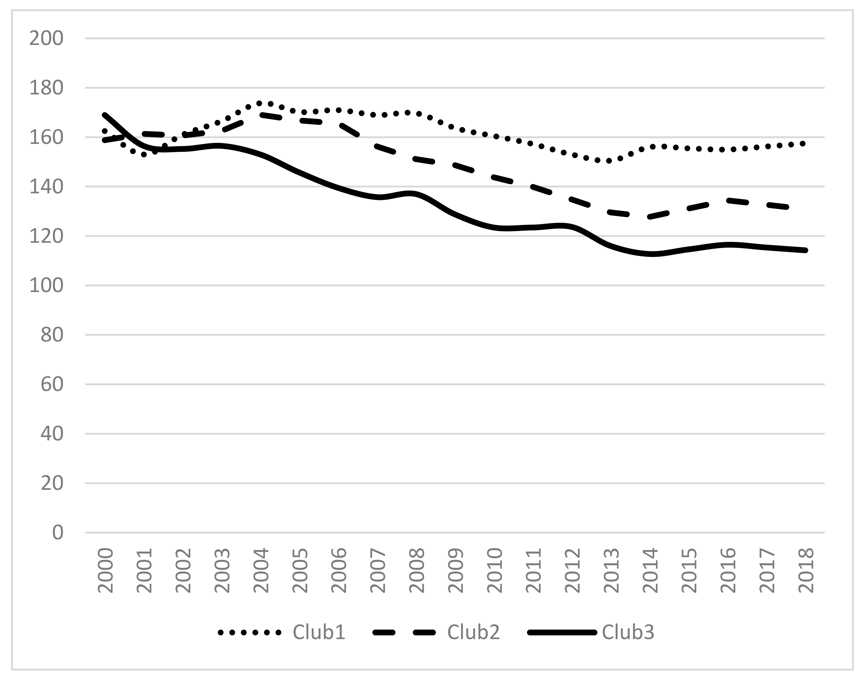
Once we have analyzed the geographical composition of the estimated convergence clubs, it seems sensible to analyze their evolution across the considered sample. To that end, Figure 3 reflects the average behavior of each one of the three estimated convergence clubs. As we can observe, the differences at the beginning of the sample are almost negligible and the three convergence clubs depart from very similar values. However, the values at the end of the sample show remarkable differences. The highest average value is given by Club 1 (158 lid), followed by Club 2 (131 lid) and Club 3 (114 lid). The average residential consumption of the regions included in Club 1 is 38% greater than that of Club 3.
We can also observe that the three estimated convergence clubs reduce household water consumption for the period 2000–2018. Club 3 does this at a remarkable average annual rate of −2.2%, whilst the declining rate of Club 2 is much more moderate (−1.1%) and is very small for Club 1 (−0.2%). This reduction is not homogenous over time. We can also find some differences if we split the sample into two periods, 2000–2008 and 2008–2018, in order to reflect the possible effect of the Great Recession. The average annual growth rates for the pre-Great Recession period are 0.5%, −0.6%, and −2.6%, respectively, for Club 1, Club 2, and Club 3. By contrast, the rates for the post-Great Recession period are −0.7%, −1.4% and −1.8%, respectively. However, we note that the aggregated behavior of Spain remains unaltered, showing a constant rate of reduction for the two subsamples considered (−1.3%), as shown in Table 1.
We can observe that the evolution of the estimated convergence clubs was different after the Great Recession, especially during the recovery period (2013–2018), given that the reduction was around −3.0% during the hardest years of this crisis (2008–2013). To illustrate this, we should note that the aggregated household water consumption of Spain grew at an annual average of 0.5% during the 2013–2018 period, whilst it plummeted (−3.0) for the 2008–2013 period (Table 1). Apparently, this is a good result in terms of sustainability. However, as Sauri [14] notes, it may also be related to the appearance of some pockets of water poverty, which would be an undesirable effect clearly associated with the Great Recession.
Having analyzed the main characteristics of the three estimated convergence clubs, we now try to determine the forces that may drive their creation.
3.2. Forces That May Drive the Convergence Club Creation
The results reported in the previous section have shown the heterogeneity of the evolution of residential consumption of water across the Spanish regions, which has implied the existence of several patterns of behavior. This section is devoted to an analysis of the forces that may drive the creation of these estimated convergence clubs. To that end, we have estimated the model:
where the dependent variable yi may have various possible outcomes, each of them related to the number of convergence clubs that the PS methodology has estimated (yi = m if the i-th region is included in the m-th convergence club, with m = 1, 2, 3.). These different values imply a preference or an ordering of the convergence clubs, which should be taken into account in the estimation. Therefore, ordered logit methods should be employed.
yi = xi’ β + ui (i = 1, 2,…, 17)
The explanatory variables (xi) have been selected from a set of general socioeconomic variables that commonly appear in the literature associated with water consumption. In this regard, we should note that authors have employed different types of variables to explain its determinants. For instance, Arbués, et al. [1], Dalhuisen, et al. [39], Sebri [40], Taylor, et al. [41], and Martínez-Espiñeira and Nauges [42] have focused on the use of economic variables. Other papers also consider the use of environmental variables, such as Domene and Sauri [43], Martínez-Espiñeira [11], Scheild and Hillenbrand [44] and Arbués and Villanúa [12]. Finally, the household structure is also considered, as can be seen in Arbués, et al. [1] and March, et al. [45], or in Marzano, et al. [46] who include household size as an explanatory variable.
Following these precedents, we have selected variables with the aim of covering these three main areas: economics (household income, price of water, secondary housing), environmental conditions (spending on environmental protection, average temperature, average rainfall), and household structure (birth rate, aging rate). We have considered two additional variables related to quality of the supply network (length of the supply network and percentage of real losses). Appendix C provides the definition and the data source of each one of these variables.
It would be interesting to use other variables that do not appear in this study but which could be investigated in future research. This is the case of the water scarcity index, the difference between houses and flats, and the percentage of houses with a garden or pool, all of which have been used in previous papers, such as those by Garrone, et al. [47]. However, these data are not currently available for the Spanish regions and, therefore, they have not been included in our set of explanatory variables.
Table 3 presents the sample average of our set of variables for each one of the estimated convergence clubs. The analysis of these values reveals very interesting insights. For instance, the regions included in Club 3 show the highest values of the household income, birth rate, spending on environmental protection, or average rainfall variables. By contrast, the average price of the water is quite similar for the three estimated convergence clubs, although it is slightly higher in Club 1. On the other hand, we can observe that the aging rate, average temperature, length of the supply network or the percentage of real losses are higher in Club 1. Finally, we should note that the household size does not seem to exhibit a high discriminating power, given that the average values for Clubs 1 and 2 are quite similar.
In order to determine which of these explanatory variables are helpful to predict why a region is included in a particular convergence club, we have estimated an ordered logit model. The final specification has been selected following a two-step procedure. We have taken into account the average values of the variables, selecting those explanatory variables that exhibit the highest power to discriminate the assignation of the regions to the estimated convergence clubs. Later, we have estimated an ordered logit model with all these variables. The final specification has been obtained by following a general-to-particular strategy where we have just maintained those variables whose estimated parameters were statistically different from 0.
The explanatory variables included in the final specification are household income, the birth rate in the different regions, and the spending on environmental protection. As we observed in Table 3, the average household income is 28.100 euros in Club 1 and rises to 35.838 in Club 3. The birth rate is 7.545 in Club 1 and rises to 8.867 in Club 3. Similarly, spending on environmental protection is 0.012% in Club 1 and rises to 0.018% in Club 3. Positive coefficients, in variables considered in the estimation shown in Table 4, imply that the probability of being included in Club 3 is higher, so the higher the values of the explanatory variables, the greater the probability of being in the convergence club that exhibits the lowest household water consumption. Finally, we should note that the pseudo R2 is relatively high (0.44), as is the percentage of correctly classified cases (a remarkable 76%). Taking into account the few observations available, this model manages largely to explain the behavior of Spanish households, and these three variables are quite helpful to discriminate the behavior of the three estimated convergence clubs.
3.3. Discussion
The results reported in the previous Section confirm the importance of income to explain the evolution of household water consumption, as reflected in the literature reviews by Arbués, et al. [1], Worthington and Hoffman [48] and Reynaud and Romano [49]. These papers show that there is a positive relationship between income and water consumption. However, we observe an inverse relationship between these two variables. The higher the per capita GDP, the lower the household water consumption per inhabitant. This appears to contradict previous results reported in the literature. Nevertheless, this can be overcome if we admit the presence of non-linearities in the income/water consumption relationship, in particular if we consider the existence of an inverted U-shape relationship, which clearly recalls the Environmental Kuznets Curve (EKC). Kuznets [50] suggested the existence of a U-shape relationship between income and inequality, which inspired some authors to analyze whether there is an inverted U-shaped relationship between environmental degradation and income. Some relatively recent papers have examined whether this EKC holds for the case of income/water consumption. The results are mostly favorable to the existence of this EKC. For instance, Duarte, et al. [51], using a sample of 65 countries; Schleich and Hillenbrand [44], who focus on the German case; and Zhao, et al. [52], who study the Chinese case, find evidence of this EKC relationship. We should note, however, that Katz [53] questions its relevance for designing water strategies, whilst Expósito, et al. [54,55] cannot find evidence of the EKC for household water consumption in the municipalities of the Guadalquivir River Basin. Finally, it is important to mention Pastor and Fullerton [56] who warn of the need to carry out a detailed analysis of the time properties of the variables, given that this can condition the use of the most appropriate econometric method.
Our results align with those which offer evidence of the existence of the EKC, suggesting the presence of a non-linear relationship between income and household water consumption. Therefore, regions with the highest per capita income levels are included in the convergence club with the lowest household water consumption. We can also associate this result with the use of water-efficient appliances, as Schleich and Hillenbrand [44] did for the German case. Those households with the highest per capita income tend to be equipped with the highest quality, newest and, therefore, the most environmentally efficient home appliances that consume less water than appliances of previous generations, which are more frequently found in low-income households. As a consequence, it comes as no surprise that several research studies have reported on the introduction of energy-saving household appliances such as efficient toilets and showers (Galarraga, et al. [57], Waris, et al. [58], Dieu-Hang, et al. [59]). Our results confirm those of Olmstead and Stavins [60], Lee and Tansel [61], Stavenhagen, et al. [62], Tortajada, et al. [20] and Suárez-Varela [63], the latter two for the Spanish case. The early replacement of older appliances by efficient models is encouraged to reduce the environmental impact in general and water savings in particular.
We should take into account that the more educated and wealthy population groups may also have greater awareness of water scarcity, the need for water conservation, and the importance of more efficient water use. This awareness may result in slower rates of increase in water consumption or even an absolute reduction in per capita water use over time, as suggested by Portnov [35]. This justifies the existence of a relationship between income and water consumption, by simply considering that the regions with the highest levels of education have the highest per capita incomes.
The second explanatory variable included in the estimated model is government spending on environmental protection. The estimated coefficient of this variable is positive and, therefore, the higher the environmental protection expenditure, the higher the probability of being included in the convergence club with the lowest household water consumption (Club 3). The presence of this variable clearly reflects the efforts made by the European Union (EU) countries to achieve greener and more sustainable economic growth. In particular, we should recall that EU Member States have made significant progress in improving the quality of Europe’s freshwater bodies through EU legislation, such as the Water Framework Directive, the Urban Wastewater Directive, and the Drinking Water Directive. These key pieces of legislation underpin the EU’s commitment to improving Europe’s water status. The aim of EU policies is to significantly reduce the negative impacts of pollution, over-abstraction and other pressures on water, and to ensure that sufficient good quality water is available for human consumption and for the environment. Our results prove that household water consumption is lower in those regions where citizens’ awareness of environmental issues is higher and, consequently, greater importance is given to the preservation of the natural environment.
Examples of this awareness about sustainable water consumption are the advertising campaigns and environmental objectives implemented by regions included in Club 3: the integrated water framework strategy of Navarra 2030, the awareness campaign carried out by the Basque Country on responsible consumption and the circular economy with the slogan “The revolution of small actions”, and the latest campaign launched by the Catalan Water Agency (ACA). Furthermore, these three regions have an agency exclusively dedicated to water management, demonstrating their commitment to sustainability. All these efforts seem to have been successful and these regions lead the reduction in household water consumption. This committed environmentalism plays an important role in water savings, as has been analyzed in Domene and Sauri [43] for the Spanish case, Gilg and Barr [64] for England, and Quentin Grafton and Jiang [65], who study the case of the Murray-Darling basin (Australia). Our results offer additional evidence that policies devoted to raising environmental awareness are very helpful to prevent the unnecessary consumption of natural resources.
The third explanatory variable included in the final specification is the birth rate, with the sign of its estimated parameter being positive. This implies that the higher the birth rate in the region, the more probable the region will be included in Club 3. This result suggests that household size is linked to household water consumption but not linearly. Rather, the presence of economies of scale seems to play some role here. Therefore, the greater the size of the household, the lower the per capita consumption, as can also be seen in Table 3. The effect of the household size on water consumption has been previously analyzed in the literature. For instance, we can cite the papers by Höglund [66], Nauges and Thomas [67], and Makki, et al. [68], who find a negative relationship between household size and household water consumption. These authors explain that this is due to the existence of the above-mentioned economies of scale and the optimum use of household appliances.
Up to this point, we have analyzed the effect of the variables whose discriminating power is high enough to appear in the final estimation. We should note, however, that there are some other relevant variables which do not appear in the final specification but may be relevant to understanding Spanish regional water consumption. Here, we are thinking especially of the price of water. We should note that, as can be seen in Table 3, the average value of this variable is similar in all the estimated convergence clubs. Then, this variable does not have enough power to predict why a region is included in a particular convergence club. To understand the absence of this relevant variable, we should take into account that water demand tends to be rather inelastic because this good has no substitutes for its basic uses, as Arbués, et al. [1], and Martínez-Espiñeira and Nauges [42] point out. In this regard, we should recall that EU water policies encourage Member States to implement better water management practices, in particular, so far as water pricing policies are concerned.
We also consider that the climate variables are relevant to understanding household water consumption. For instance, the results of Portnov [35] show that per capita water consumption tends to be higher in warm and dry places. This appears to be verified by the Spanish case, given that the regions in Club 1 are warmer and drier than those included in Club 3. In spite of this fact, these variables do not appear in the final specification of the model. Something similar occurs in the case of the length of the supply network and the percentage of real losses in the water supplied. This lack of discriminating power may be explained by considering that the cross-section sample is small and there are not enough degrees of freedom to include a larger group of explanatory variables in the final estimation. Then, we should recall that the data limitations are important in this study and the results should be interpreted with some caution. This being the case, we should also remark that the final specification includes the variables with the highest discriminating power.
4. Conclusions
The aim of this paper is to study the evolution of household water consumption in Spain, paying special attention to the analysis of possible regional differences. To that end, we have considered the per capita annual consumption of water of households for the different Spanish regions. The use of the methodology proposed in Phillips and Sul [18,19] leads us to conclude that Spanish regional household water consumption is so heterogeneous that the existence of a single pattern of behavior between the Spanish regions can be rejected.
Rather, we can observe the existence of three statistically different convergence clubs. Navarra, the País Vasco, La Rioja, and Cataluña are the regions included in Club 3, the one with the lowest consumption. By contrast, the Islas Canarias, Comunidad Valenciana, Castilla y León and Cantabria are included in the convergence club that shows the highest levels of consumption.
In order to understand the creation of these convergence clubs, we have estimated an ordered logit model which reveals that the household income, the percentage of expenditure on environmental protection and the birth rate are crucial to explain the water consumption disparities.
These variables are very useful for designing more efficient policies aimed at promoting savings in household consumption. In particular, our results show that these policies should be sustained on two pillars. First, it is crucial to help households to renew and improve their home appliances. Secondly, we have also found that public spending on environmental protection is essential for lower household water consumption, given that it creates environmental awareness, which has a great impact on such consumption. This highlights the importance of environmental and socioeconomic policies to combat water scarcity. By contrast, our results also suggest that policies based solely on prices do not seem very efficient in reducing Spanish household water consumption.
It should be noted that this research has employed a time series perspective, instead of the more standard cross-sectional view. This type of analysis has some advantages, especially related to the inclusion of the time dimension, which allows us to provide a time consistency to the results and to include the dynamic nature of the variables in the analysis. However, we should also be aware of its limitations, some of which are related to the short length of the series. This problem will be solved once longer series are available.
Finally, we should be aware that the recent COVID-19 pandemic may have affected citizen’s habits. We should especially take into account that most countries have fought the pandemic by confining their population in their homes. It is quite probable that this might have altered water consumption patterns of behavior. It would, therefore, be of considerable interest to study water consumption in the years after 2018 and analyze the behavior of households in the period of the Coronavirus confinement, when the relevant data becomes available. In this regard, a comparison with other regions or between different countries is limited by the absence of a homogeneous international database on household water consumption. If this were created, it could be of great interest to extend our study to other regions and obtain a better picture of the evolution of water consumption habits in other areas.
Author Contributions
Data curation, B.B.; Investigation, M.B.S.-F.; Methodology, A.M.; Writing—original draft, B.B.; Writing—Review & Editing, A.M. and M.B.S.-F. All authors have read and agreed to the published version of the manuscript.
Funding
This work was supported by the “Fundación Caja Rural de Aragón” Chair of the University of Zaragoza (Spain), by the Ministerio de Ciencia e Innovación, grant PID2020-113229RB-C44 and by the Aragonese Government (grant: Cassetem).
Institutional Review Board Statement
Not applicable.
Informed Consent Statement
Not applicable.
Acknowledgments
The authors would like to thank three anonymous referees for their useful suggestions and comments. The usual disclaimer applies.
Conflicts of Interest
The authors declare no conflict of interest.
Appendix A
| Author | Econometric Technique | Data | Result |
| Nauges and Thomas [67] | Panel data | 116 municipalities of Eastern France | Analyzes the effect of the public/private utilities on water demand. |
| Portnov and Meir [35] | β -convergence | 160 urban localities, Israel | Convergence or divergence in urban water consumption in Israel. |
| Schleich and Hillenbrand [44] | Cross-sectional estimation | 600 water supply areas, Germany | Price and income are relevant variables. |
| Fielding, et al. [69] | Cross-sectional estimation | 1008 households in Queensland, Australia | Demographic, psychosocial, behavioral, and infrastructure variables all have a role to play in determining household water use. |
| Wolters [70] | Cross-sectional estimation | Survey of families in Oregon, USA | The interaction of environmental concern and sociodemographics that predict identified water conservation behaviors is observed. |
| Katz [53] | Panel data | 30 OECD countries and 50 USA states. | Some support to the Environmental Kuznetz Curve. |
| Tzeremes and Tzeremes [34] | Phillips-Sul convergence analysis | 30 major U.S. cities | They find divergence, but also evidence in favor of convergence clubs. |
| Zhang, et al. [71] | Input-Ouput Tables | Chinese provinces | Important virtual scarce water differences are found across the Chinese provinces. |
| Acuña, et al. [36] | β -convergence | 348 Chilean localities from 2010 to 2015 | Shows convergence in water consumption. |
| Rondinel-Oviedo and Sarmiento-Pastor [72] | Cross-sectional analysis | Lima metropolitan area, Peru | Water use related to behavior, attitude or education is conditioned by dwelling characteristics and the types of devices employed in bathrooms. |
| Russell and Knoeri [73] | Cross-sectional estimation (hierarchical regression) | 1196 households across the UK | Attitudes, norms and habits play an important role in determining intention to conserve water. |
| Abu-Bakar, et al. [74] | Cluster analysis | 11,528 households, UK | Existence of different patterns of behavior. |
Appendix B. Phillips-Sul Clustering Algorithm
The estimated convergence clubs have been obtained by using the PS clustering algorithm, which is based on the following steps:
- Order the N regions according to their final values.
- Starting from the highest-order state, add adjacent regions from our ordered list and estimate model (3). Then, select the core group by maximizing the value of the convergence t-statistic, subject to the restriction that it is greater than −1.65.
- Continue adding one state at a time of the remaining regions to the core group, and re-estimate model (3) for each formation. Use the sign criterion (t-statistic > 0) to decide whether a state should join the core group.
- For the remaining regions, repeat steps (ii)–(iii) iteratively and stop when convergence clubs can no longer be formed. If the last group does not have a convergence pattern, conclude that its members diverge.
Appendix C. Definition of Variables
- Household income: Average annual net household income by regions. Source: National Statistical Institute of Spain (INE).
- Birth rate: Ratio between the number of observed births and the average population for each year by region. Source: National Statistical Institute of Spain (INE).
- Spending on environmental protection. (Percentage of total public spending dedicated to environmental protection.) Source: National Statistical Institute of Spain (INE).
- Price of water: Quotient between the amounts paid for water supply plus the amounts paid for sewerage, purification and sanitation or discharge charges, and the volume of water registered and distributed to users. Source: National Statistical Institute of Spain (INE).
- Aging index: Ratio (in percent) between the population over 64 years of age and the population under 16 years of age. Source: National Statistical Institute of Spain (INE).
- Average temperature: Statistical averages obtained between maximum and minimum temperatures. Source: State Meteorological Agency (Aemet).
- Average rainfall: Average rainfall recorded during a year at meteorological stations. Source: State Meteorological Agency (Aemet).
- Length of the supply network: Ratio measured in meters per inhabitant. Source: National Statistical Institute of Spain (INE).
- Percentage of real losses: Physical losses of water that occur in the public supply network up to the user’s metering point. It includes water leaks, breaks, tank overflows and breakdowns in the distribution network and in users’ connections. Source: National Statistical Institute of Spain (INE).
- Second homes: This is used during only part of the year on a seasonal, periodic, or sporadic basis and is not the usual residence of one or more persons. Source: National Statistical Institute of Spain (INE).
- Household size: Percentage of households out of the total for each of the measured sizes (less than 75 square meters, less than 105 square meters and less than 150 square meters). Source: National Statistical Institute of Spain (INE).
References
- Arbués, F.; García-Valiñas, M.Á.; Martínez-Espiñeira, R. Estimation of residential water demand: A state-of-the-art review. J. Socio-Econ. 2003, 32, 81–102. [Google Scholar] [CrossRef]
- Marshall, A. Water as an Element of National Wealth. In Memorials of Alfred Marshall; Kelley & Millman: New York, NY, USA, 1956; pp. 134–141. [Google Scholar]
- Hutton, G.; Varughese, M. The Costs of Meeting the 2030 Sustainable Development Goal Targets on Drinking Water, Sanitation, and Hygiene; Water and Sanitation Program: Technical Paper; World Bank: Washington, DC, USA, 2016. [Google Scholar]
- United Nations World Water Development Report 2021: Valuing Water; Nesco: Paris, France, 2021.
- Ho, L.; Alonso, A.; Forio, M.A.E.; Vanclooster, M.; Goethals, P.L. Water research in support of the Sustainable Development Goal 6: A case study in Belgium. J. Clean. Prod. 2020, 277, 124082. [Google Scholar] [CrossRef]
- Hoekstra, A.Y.; Chapagain, A.K.; Van Oel, P.R. Advancing water footprint assessment research: Challenges in monitoring progress towards sustainable development goal 6. Water 2017, 9, 438. [Google Scholar] [CrossRef] [Green Version]
- Hofste, R.W.; Reig, P.; Schleifer, L. 17 Countries, Home to One-Quarter of the World’s Population, Face Extremely High Water Stress; World Resources Institute: Washington, DC, USA, 2019. [Google Scholar]
- Cazcarro, I.; Duarte, R.; Sánchez-Chóliz, J. Economic growth and the evolution of water consumption in Spain: A structural decomposition analysis. Ecol. Econ. 2013, 96, 51–61. [Google Scholar] [CrossRef]
- Estrela, T.; Pérez-Martin, M.A.; Vargas, E. Impacts of climate change on water resources in Spain. Hydrol. Sci. J. 2012, 57, 1154–1167. [Google Scholar] [CrossRef]
- Gracia-De-Rentería, P.; Barberán, R.; Mur, J. Urban water demand for industrial uses in Spain. Urban Water J. 2019, 16, 114–124. [Google Scholar] [CrossRef]
- Martínez-Espiñeira, R. Residential water demand in the Northwest of Spain. Environ. Resour. Econ. 2002, 21, 161–187. [Google Scholar] [CrossRef]
- Arbués, F.; Villanúa, I. Potential for pricing policies in water resource management: Estimation of urban residential water demand in Zaragoza, Spain. Urban Stud. 2006, 43, 2421–2442. [Google Scholar] [CrossRef]
- Hoyos, D.; Artabe, A. Regional differences in the price elasticity of residential water demand in Spain. Water Resour. Manag. 2017, 31, 847–865. [Google Scholar] [CrossRef]
- Sauri, D. The decline of water consumption in Spanish cities: Structural and contingent factors. Int. J. Water Resour. Dev. 2020, 36, 909–925. [Google Scholar] [CrossRef]
- Fuentes, E.; Arce, L.; Salom, J. A review of domestic hot water consumption profiles for application in systems and buildings energy performance analysis. Renew. Sustain. Energy Rev. 2018, 81, 1530–1547. [Google Scholar] [CrossRef]
- Bich-Ngoc, N.; Teller, J. A review of residential water consumption determinants. In Proceedings of the International Conference on Computational Science and Its Applications, Melbourne, Australia, 2–5 June 2018; Springer International Publishing: Cham, Switzerland, 2018; pp. 685–696. [Google Scholar]
- Abu-Bakar, H.; Williams, L.; Hallett, S.H. A review of household water demand management and consumption measurement. J. Clean. Prod. 2021, 292, 125872. [Google Scholar] [CrossRef]
- Phillips, P.C.; Sul, D. Transition modeling and econometric convergence tests. Econometrica 2007, 75, 1771–1855. [Google Scholar] [CrossRef] [Green Version]
- Phillips, P.C.; Sul, D. Economic transition and growth. J. Appl. Econom. 2009, 24, 1153–1185. [Google Scholar] [CrossRef] [Green Version]
- Tortajada, C.; González-Gómez, F.; Biswas, A.K.; Buurman, J. Water demand management strategies for water-scarce cities: The case of Spain. Sustain. Cities Soc. 2019, 45, 649–656. [Google Scholar] [CrossRef]
- Barro, R.J.; Sala-i-Martin, X. Convergence. J. Political Econ. 1992, 100, 223–251. [Google Scholar] [CrossRef]
- Carlino, G.A.; Mills, L. Are US regional incomes converging? A time series analysis. J. Monet. Econ. 1993, 32, 335–346. [Google Scholar] [CrossRef]
- Bernard, A.B.; Durlauf, S.N. Convergence in international output. J. Appl. Econom. 1995, 10, 97–108. [Google Scholar] [CrossRef] [Green Version]
- González-Álvarez, M.A.; Lázaro-Alquézar, A.; Simón-Fernández, M.B. Global Trends in Child Obesity: Are Figures Converging? Int. J. Environ. Res. Public Health 2020, 17, 9252. [Google Scholar] [CrossRef] [PubMed]
- Clemente, J.; Lázaro-Alquézar, A.; Montañés, A. US State health expenditure convergence: A revisited analysis. Econ. Model. 2019, 83, 210–220. [Google Scholar] [CrossRef] [Green Version]
- Rodríguez-Benavides, D.; López-Herrera, F.; Venegas-Martínez, F. Are there economic convergence clubs in Latin America? J. Econ. Dev. Stud. 2014, 2, 113–123. [Google Scholar] [CrossRef]
- Jangam, B.P.; Sahoo, P.K.; Akram, V. Convergence in electricity consumption across Indian states: A disaggregated analysis. Int. J. Energy Sect. Manag. 2019, 14, 624–637. [Google Scholar] [CrossRef]
- Camarero, M.; Picazo-Tadeo, A.J.; Tamarit, C. Are the determinants of CO2 emissions converging among OECD countries? Econ. Lett. 2013, 118, 159–162. [Google Scholar] [CrossRef] [Green Version]
- Parker, S.; Bhatti, M.I. Dynamics and drivers of per capita CO2 emissions in Asia. Energy Econ. 2020, 89, 104798. [Google Scholar] [CrossRef]
- Apergis, N.; Payne, J.E. NAFTA and the convergence of CO2 emissions intensity and its determinants. Int. Econ. 2020, 161, 1–9. [Google Scholar] [CrossRef]
- Payne, J.E.; Apergis, N. Convergence of per capita carbon dioxide emissions among developing countries: Evidence from stochastic and club convergence tests. Environ. Sci. Pollut. Res. 2020, 28, 1–13. [Google Scholar] [CrossRef] [PubMed]
- Camarero, M.; Castillo, J.; Picazo-Tadeo, A.J.; Tamarit, C. Eco-efficiency and convergence in OECD countries. Environ. Resour. Econ. 2013, 55, 87–106. [Google Scholar] [CrossRef] [Green Version]
- Alcay, A.; Montañés, A.; Simón-Fernández, M.B. Waste generation in Spain. Do Spanish regions exhibit a similar behavior? Waste Manag. 2020, 112, 66–73. [Google Scholar] [CrossRef] [PubMed]
- Tzeremes, P.; Tzeremes, N.G. A convergence assessment of water price rates: Evidence from major US cities. Lett. Spat. Resour. Sci. 2018, 11, 361–368. [Google Scholar] [CrossRef]
- Portnov, B.A.; Meir, I. Urban water consumption in Israel: Convergence or divergence? Environ. Sci. Policy 2008, 11, 347–358. [Google Scholar] [CrossRef]
- Acuña, G.I.; Echeverría, C.; Godoy, A.; Vásquez, F. The role of climate variability in convergence of residential water consumption across Chilean localities. Environ. Econ. Policy Stud. 2020, 22, 89–108. [Google Scholar] [CrossRef]
- Quah, D. Galton’s fallacy and tests of the convergence hypothesis. Scand. J. Econ. 1993, 11, 427–443. [Google Scholar] [CrossRef]
- Hodrick, R.J.; Prescott, E.C. Postwar US business cycles: An empirical investigation. J. Money Credit. Bank. 1997, 29, 1–16. [Google Scholar] [CrossRef]
- Dalhuisen, J.M.; Florax, R.J.; De Groot, H.L.; Nijkamp, P. Price and income elasticities of residential water demand: A meta-analysis. Land Econ. 2003, 79, 292–308. [Google Scholar] [CrossRef]
- Sebri, M. A meta-analysis of residential water demand studies. Environ. Dev. Sustain. 2014, 16, 499–520. [Google Scholar] [CrossRef]
- Taylor, R.G.; McKean, J.R.; Young, R.A. Alternate price specifications for estimating residential water demand with fixed fees. Land Econ. 2004, 80, 463–475. [Google Scholar] [CrossRef]
- Martínez-Espiñeira, R.; Nauges, C. Is really all domestic water consumption sensitive to price control? Appl. Econ. 2004, 36, 1697–1703. [Google Scholar] [CrossRef]
- Domene, E.; Sauri, D. Urbanisation and water consumption: Influencing factors in the metropolitan region of Barcelona. Urban Stud. 2006, 43, 1605–1623. [Google Scholar] [CrossRef]
- Schleich, J.; Hillenbrand, T. Determinants of residential water demand in Germany. Ecol. Econ. 2009, 68, 1756–1769. [Google Scholar] [CrossRef] [Green Version]
- March, H.; Perarnau, J.; Sauri, D. Exploring the links between immigration, ageing and domestic water consumption: The case of the Metropolitan Area of Barcelona. Reg. Stud. 2012, 46, 229–244. [Google Scholar] [CrossRef]
- Marzano, R.; Rouge, C.; Garrone, P.; Grilli, L.; Harou, J.J.; Pulido-Velazquez, M. Determinants of the price response to residential water tariffs: Meta-analysis and beyond. Environ. Model. Softw. 2018, 101, 236–248. [Google Scholar] [CrossRef]
- Garrone, P.; Grilli, L.; Marzano, R. Price elasticity of water demand considering scarcity and attitudes. Util. Policy 2019, 59, 100927. [Google Scholar] [CrossRef]
- Worthington, A.C.; Hoffman, M. An empirical survey of residential water demand modelling. J. Econ. Surv. 2008, 22, 842–871. [Google Scholar] [CrossRef] [Green Version]
- Reynaud, A.; Romano, G. Advances in the economic analysis of residential water use: An introduction. Water 2018, 10, 1162. [Google Scholar] [CrossRef] [Green Version]
- Kuznets, S. Economic growth and income inequality. Am. Econ. Rev. 1995, 45, 1–28. [Google Scholar]
- Duarte, R.; Pinilla, V.; Serrano, A. Is there an environmental Kuznets curve for water use? A panel smooth transition regression approach. Econ. Model. 2013, 31, 518–527. [Google Scholar] [CrossRef] [Green Version]
- Zhao, X.; Fan, X.; Liang, J. Kuznets type relationship between water use and economic growth in China. J. Clean. Prod. 2017, 168, 1091–1100. [Google Scholar] [CrossRef]
- Katz, D. Water use and economic growth: Reconsidering the environmental Kuznets curve relationship. J. Clean. Prod. 2015, 88, 205–213. [Google Scholar] [CrossRef]
- Expósito, A.; Pablo-Romero, M.; Sánchez-Braza, A. Testing EKC for urban water use: Empirical evidence at River Basin scale from the Guadalquivir River, Spain. J. Water Resour. Plan. Manag. 2019, 145, 04019005. [Google Scholar] [CrossRef]
- Expósito, A.; Pablo-Romero, M.D.P.; Sánchez-Braza, A. Exploring EKCs in Urban Water and Energy Use Patterns and Its Interconnections: A Case Study in Southern Spain. In Sustaining Resources for Tomorrow; Springer International Publishing: Cham, Switzerland, 2020; pp. 47–65. [Google Scholar]
- Pastor, D.J.; Fullerton, T.M. Municipal Water Consumption and Urban Economic Growth in El Paso. Water 2020, 12, 2656. [Google Scholar] [CrossRef]
- Galarraga, I.; Abadie, L.M.; Kallbekken, S. Designing incentive schemes for promoting energy-efficient appliances: A new methodology and a case study for Spain. Energy Policy 2016, 90, 24–36. [Google Scholar] [CrossRef]
- Waris, I.; Hameed, I. Promoting environmentally sustainable consumption behavior: An empirical evaluation of purchase intention of energy-efficient appliances. Energy Effic. 2020, 13, 1653–1664. [Google Scholar] [CrossRef]
- Dieu-Hang, T.; Grafton, R.Q.; Martínez-Espiñeira, R.; Garcia-Valiñas, M. Household adoption of energy and water-efficient appliances: An analysis of attitudes, labelling and complementary green behaviours in selected OECD countries. J. Environ. Manag. 2017, 197, 140–150. [Google Scholar] [CrossRef] [PubMed]
- Olmstead, S.M.; Stavins, R.N. Comparing price and nonprice approaches to urban water conservation. Water Resour. Res. 2009, 45. [Google Scholar] [CrossRef] [Green Version]
- Lee, M.; Tansel, B. Life cycle based analysis of demands and emissions for residential water-using appliances. J. Environ. Manag. 2012, 101, 75–81. [Google Scholar] [CrossRef] [PubMed]
- Stavenhagen, M.; Buurman, J.; Tortajada, C. Saving water in cities: Assessing policies for residential water demand management in four cities in Europe. Cities 2018, 79, 187–195. [Google Scholar] [CrossRef]
- Suárez-Varela, M. Modeling residential water demand: An approach based on household demand systems. J. Environ. Manag. 2020, 261, 109921. [Google Scholar] [CrossRef] [PubMed]
- Gilg, A.; Barr, S. Behavioural attitudes towards water saving? Evidence from a study of environmental actions. Ecol. Econ. 2006, 57, 400–414. [Google Scholar] [CrossRef]
- Quentin Grafton, R.; Jiang, Q. Economic effects of water recovery on irrigated agriculture in the Murray-Darling Basin. Aust. J. Agric. Resour. Econ. 2011, 55, 487–499. [Google Scholar] [CrossRef] [Green Version]
- Höglund, L. Household demand for water in Sweden with implications of a potential tax on water use. Water Resour. Res. 1999, 35, 3853–3863. [Google Scholar] [CrossRef]
- Nauges, C.; Thomas, A. Privately operated water utilities, municipal price negotiation, and estimation of residential water demand: The case of France. Land Econ. 2000, 76, 68–85. [Google Scholar] [CrossRef]
- Makki, A.A.; Stewart, R.A.; Beal, C.D.; Panuwatwanich, K. Novel bottom-up urban water demand forecasting model: Revealing the determinants, drivers and predictors of residential indoor end-use consumption. Resour. Conserv. Recycl. 2015, 95, 15–37. [Google Scholar] [CrossRef] [Green Version]
- Fielding, K.S.; Russell, S.; Spinks, A.; Mankad, A. Determinants of household water conservation: The role of demographic, infrastructure, behavior, and psychosocial variables. Water Resour. Res. 2012, 48. [Google Scholar] [CrossRef] [Green Version]
- Wolters, E.A. Attitude–behavior consistency in household water consumption. Soc. Sci. J. 2014, 51, 455–463. [Google Scholar] [CrossRef]
- Zhang, Y.; Chen, Y.; Huang, M. Water footprint and virtual water accounting for China using a multi-regional input-output model. Water 2018, 11, 34. [Google Scholar] [CrossRef] [Green Version]
- Rondinel-Oviedo, D.R.; Sarmiento-Pastor, J.M. Water: Consumption, usage patterns, and residential infrastructure. A comparative analysis of three regions in the Lima metropolitan area. Water Int. 2020, 45, 824–846. [Google Scholar] [CrossRef]
- Russell, S.V.; Knoeri, C. Exploring the psychosocial and behavioural determinants of household water conservation and intention. Int. J. Water Resour. Dev. 2020, 36, 940–955. [Google Scholar] [CrossRef] [Green Version]
- Abu-Bakar, H.; Williams, L.; Hallett, S.H. Quantifying the impact of the COVID-19 lockdown on household water consumption patterns in England. NPJ Clean Water 2021, 4, 1–9. [Google Scholar] [CrossRef]
Figure 1.
σ-convergence analysis. (a) Standard deviation. (b) Coefficient of variation.

Figure 2.
Estimated convergence clubs.

Figure 3.
Average values of the regions in the estimated convergence clubs. This figure presents the evolution of the average household water consumption of the estimated convergence clubs.
Figure 3.
Average values of the regions in the estimated convergence clubs. This figure presents the evolution of the average household water consumption of the estimated convergence clubs.


Table 1.
Descriptive analysis. Household consumption of water (liters/inhabitant/day).
| Region | Acronym | 2000 | 2018 | Min | Max | g0018 | g0008 | g0813 | g1318 |
|---|---|---|---|---|---|---|---|---|---|
| Andalucía | AND | 184 | 128 | 120 | 196 | −2.0% | −2.2% | −4.9% | 1.3% |
| Aragón | ARA | 174 | 129 | 129 | 174 | −1.6% | −2.2% | −2.4% | 0.0% |
| Asturias | AST | 152 | 140 | 122 | 187 | −0.5% | 1.8% | −7.0% | 2.8% |
| Islas Baleares | BAL | 132 | 121 | 120 | 152 | −0.5% | 0.5% | 0.6% | −3.0% |
| Islas Canarias | CAN | 143 | 135 | 135 | 159 | −0.3% | 1.3% | −2.1% | −1.1% |
| Cantabria | CAB | 187 | 172 | 144 | 202 | −0.5% | −0.2% | −4.8% | 3.6% |
| Castilla y León | CYL | 154 | 148 | 146 | 173 | −0.2% | −0.3% | 0.9% | −1.2% |
| Castilla-La Mancha | CLM | 186 | 135 | 125 | 200 | −1.8% | −2.7% | −1.2% | −0.7% |
| Cataluña | CAT | 185 | 123 | 117 | 185 | −2.2% | −3.8% | −3.0% | 1.0% |
| C. Valenciana | CVA | 166 | 175 | 152 | 188 | 0.3% | 1.4% | −3.2% | 2.1% |
| Extremadura | EXT | 158 | 126 | 125 | 185 | −1.2% | −0.2% | −2.1% | −2.1% |
| Galicia | GAL | 130 | 125 | 119 | 161 | −0.2% | 1.4% | −3.9% | 1.0% |
| Madrid | MAD | 171 | 125 | 125 | 171 | −1.7% | −2.4% | −1.5% | −0.9% |
| Murcia | MUR | 142 | 149 | 124 | 166 | 0.3% | 1.3% | −4.6% | 3.7% |
| Navarra | NAV | 157 | 114 | 111 | 157 | −1.8% | −2.6% | −2.5% | 0.4% |
| País Vasco | PAV | 155 | 104 | 104 | 155 | −2.2% | −1.5% | −2.1% | −3.3% |
| La Rioja | LAR | 179 | 116 | 106 | 179 | −2.4% | −2.3% | −5.4% | 0.7% |
| España | SPA | 168 | 133 | 130 | 173 | −1.3% | −1.3% | −3.0% | 0.5% |
This table presents a descriptive analysis of the household consumption of water (measured in liters per inhabitant per day) for the 17 Spanish regions and the total value of Spain. The columns 2000 and 2018 represent the values at the beginning and at the end of the sample, respectively. The columns min and max are the minimum and maximum values of the sample, respectively. The last four columns (g0018, g0008, g0813 and g1318) present the annual average growth rate for the periods 2000–2018, 2000–2008, 2008–2013 and 2013–2018, respectively.
Table 2.
Testing for convergence.
| Panel I. Testing for Convergence | ||||||
|---|---|---|---|---|---|---|
| −1.68 | ||||||
| Log t-ratio | −27.54 | |||||
| Panel II. Estimated Convergence Clubs | ||||||
| Initial convergence clubs | Merging convergence club analysis | Final convergence clubs | ||||
| Club 1 | CAN, CAB, CYL, CVAL | 0.017 (0.180) | Club 1 | CAN, CAB, CYL, CVAL | ||
| Club 2 | AND, ARA, AST, BAL, CLM, EXT, GAL, MAD, MUR | 0.523 (3.300) | Club 1 + 2 | −1.458 (−11.861) | Club 2 | AND, ARA, AST, BAL, CLM, EXT, GAL, MAD, MUR |
| Club 3 | CAT, NAV, PAV, LAR | 0.194 (1.880) | Club 2 +3 | −0.877 (−18.120) | Club 3 | CAT, NAV, PAV, LAR |
This table reflects the results of the use of the methodology proposed in Phillips and Sul [18]. Panel I presents the estimation of Equation (3) for the total sample. Panel II shows the results of the application of the cluster algorithm. Columns 3 and 5 reflect the estimated coefficients (upper value) and the corresponding log t-ratio resulting from the estimation of Equation (3) for the initial estimated convergence clubs and the merged convergence clubs, respectively. The regions are Andalucía (AND), Aragón (ARA), Asturias (AST), Islas Baleares (BAL), Islas Canarias (CAN), Cantabria (CAB), Castilla y León (CYL), Castilla-La Mancha (CLM), Cataluña (CAT), Comunidad Valenciana (CVA), Extremadura (EXT), Galicia (GAL), Comunidad de Madrid (MAD), Región de Murcia (MUR), Comunidad Foral de Navarra (NAV), País Vasco (PAV) and La Rioja (LAR).
Table 3.
Average values of the explanatory variables of the estimated convergence clubs.
| Variable | Club 1 | Club 2 | Club 3 |
|---|---|---|---|
| Household income | 28,100 | 29,754 | 35,838 |
| Birth rate | 7.54 | 8.59 | 8.87 |
| Spending on environmental protection | 0.012 | 0.014 | 0.018 |
| Price of water | 1.85 | 1.72 | 1.78 |
| Aging rate | 136.93 | 128.11 | 124.36 |
| Average temperature | 17.12 | 16.89 | 14.67 |
| Average rainfall | 498.88 | 455.24 | 683.10 |
| Length of the supply network | 7.40 | 5.78 | 5.00 |
| Percentage of real losses | 20.90 | 15.86 | 15.30 |
| Secondary housing | 0.28 | 0.36 | 0.37 |
| Households <75 m2 | 25.88 | 24.71 | 28.95 |
| Households <105 m2 | 42.42 | 41.65 | 44.71 |
| Households <150 m2 | 18.03 | 20.19 | 14.93 |
The table presents the average values of the different variables for each one of the estimated convergence clubs.
Table 4.
Estimation of the ordered logit model.
| Variable | Estimation |
|---|---|
| Household income | 4.277 × (10−4) (2.58) |
| Birth rate | 1.42 (2.76) |
| Spending on environmental protection | 192.62 (1.85) |
| Pseudo R2 | 0.4402 |
| % Cases correctly classified | 76% |
This table reflects the results of the ordered logit estimation of Equation (4). The dependent variable takes the value i when the region is included in convergence club i, with i = 1, 2, 3. The values in parenthesis are the robust t-statistics for testing the null hypothesis that the associated coefficient is 0.
Publisher’s Note: MDPI stays neutral with regard to jurisdictional claims in published maps and institutional affiliations. |
© 2022 by the authors. Licensee MDPI, Basel, Switzerland. This article is an open access article distributed under the terms and conditions of the Creative Commons Attribution (CC BY) license (https://creativecommons.org/licenses/by/4.0/).
Share and Cite
MDPI and ACS Style
Baigorri, B.; Montañés, A.; Simón-Fernández, M.B. Household Water Consumption in Spain: Disparities between Region. Water 2022, 14, 1121. https://doi.org/10.3390/w14071121
AMA Style
Baigorri B, Montañés A, Simón-Fernández MB. Household Water Consumption in Spain: Disparities between Region. Water. 2022; 14(7):1121. https://doi.org/10.3390/w14071121
Chicago/Turabian StyleBaigorri, Bárbara, Antonio Montañés, and María Blanca Simón-Fernández. 2022. "Household Water Consumption in Spain: Disparities between Region" Water 14, no. 7: 1121. https://doi.org/10.3390/w14071121
Note that from the first issue of 2016, this journal uses article numbers instead of page numbers. See further details here.