
Optimizing Parameters for the Downscaling of Daily Precipitation in Normal and Drought Periods in South Korea


Department of Civil and Environmental Engineering, Sejong University, Seoul 05006, Korea
*
Author to whom correspondence should be addressed.
Water 2022, 14(7), 1108; https://doi.org/10.3390/w14071108
Submission received: 9 February 2022
/
Revised: 28 March 2022
/
Accepted: 29 March 2022
/
Published: 30 March 2022
(This article belongs to the Special Issue Assessing and Managing Risk of Flood and Drought in a Changing World)
Abstract
:One important factor that affects the performance of statistical downscaling methods is the selection of appropriate parameters. However, no research on the optimization of downscaling parameters has been conducted in South Korea to date, and existing parameter selection methods are dependent on studies conducted in other regions. Moreover, several large-scale predictors have been used to predict abnormal phenomena such as droughts, but in the field of downscaling, parameter optimization methods that are suitable for drought conditions have not yet been developed. In this study, by using the K-nearest analog methodology, suitable daily precipitation downscaling parameters for normal and drought periods were derived. The predictor variables, predictor domain, analog date size, time dependence parameters, and parameter sensitivity values that are representative of South Korea were presented quantitatively. The predictor variables, predictor domain, and analog date size were sensitive to the downscaling performance in that order, but the time dependency did not affect the downscaling process. Regarding calibration, the downscaling results obtained based on the drought parameters returned smaller root mean square errors of 1.3–28.4% at approximately 70% of the stations compared to those of the results derived based on normal parameters, confirming that drought parameter-based downscaling methods are reasonable. However, as a result of the validation process, the drought parameter stability was lower than the normal parameter stability. In the future, further studies are needed to improve the stability of drought parameters.
1. Introduction
In recent decades, climate change has caused unusual extreme climate conditions all over the world. Numerous studies have reported that the flood and drought damage probability will increase in the future [1,2,3]. One of the most rational means for simulating climate change involves the use of global climate models (GCMs); most climate change studies conducted over the past decades have been based on GCMs [4,5,6]. However, since GCMs have spatial resolutions ranging from 100 to 300 km, limitations arise when using these models to simulate spatial variabilities in regional-scale climate conditions across basins, cities, etc. [7,8,9]. To address these scale mismatches, dynamic and statistical downscaling methods have been developed over the past few decades [10,11,12].
Dynamic downscaling methods have advantages in that they can produce physically consistent results. However, the lengths of data series and the ensemble members of dynamic downscaling results are often limited because considerable input data, computational resources, and professional human intervention are required to conduct these simulations. These limitations prevent the application of dynamic downscaling results in fields such as water resources, agriculture, and ecology, in which experiments are conducted with regard to various aspects [13,14,15]. Statistical downscaling methods, which are inexpensive and easily applied with simple methods, have been used in these applied fields [15]. One of the most popular statistical downscaling approaches is the analog method, which has achieved satisfactory performance despite its simple structure [13,16,17]. The analog method is based on historical analog dates with synoptic weather patterns similar to those of the target dates.
One common analog approach is the K-nearest analog method; in this method, K analog dates are adopted for the downscaling process [18]. Since this method was first developed, several attempts have been made to improve the analog methodology [16,19,20,21]. One of these attempts involved exploring parameters aiming to improve the performance of the analog method [22]. In analog downscaling, appropriate parameters should be applied in consideration of the regional synoptic weather patterns [22]. Some parameters that are highly sensitive to the downscaling performance include the predictor variable, predictor domain, analog date size used for downscaling, and time dependency [22].
Several studies have attempted to optimize the parameters listed above in specific regions [20,23,24,25,26,27]. Trial and error methods have generally been applied to this parameter selection process, and when multiple parameters are desired, a sequential process is used to search for each parameter incrementally [24,26]. In addition, global optimization has been performed based on vast computational resources to consider the combined effects of various parameters [26]. Most of these studies have been conducted in certain countries, such as Australia, France, and Switzerland [23,24,25,26], while few investigations have been conducted in Asia [27,28].
In South Korea, past studies have explored spatial downscaling predictors [29,30]. In past research, the geopotential at the 500 pressure level, mean sea surface pressure, air temperature at the 850 pressure level, and zonal and meridional wind speeds at the 200 pressure level were selected as rainfall and temperature predictors. However, these predictors were searched for by hindcasting with predictive models, and the results thus contained bias and returned potential predictors at few pressure levels. Precipitation and surface temperature were used as predictors to apply the bias-corrected constructed analog (BCCA) and multivariate adapted constructed analog (MACA) methodologies [13]. However, exploratory research on parameters other than predictor variables has not yet been conducted. Because different weather patterns occur in different regions, selecting downscaling parameters based on studies representing other regions may negatively affect the downscaling performance. Because parameter-search research results can be used as fundamental data not only for analog downscaling research but also for other downscaling approaches, parameter selection research in South Korea is critical.
In applications such as water resources, some studies have been conducted on abnormal periods that cause more significant socioeconomic risks than normal phenomena. In particular, climate change impact assessments related to drought have been conducted in various aspects based on results obtained with GCMs [5,31,32]. Therefore, downscaling studies considering drought conditions need to be conducted, but studies involving searches for analog parameters have been conducted only for normal periods thus far. Drought prediction research has suggested that synoptic weather variables, which represent large-scale weather patterns, are commonly used as predictors to predict drought situations [33,34]. In addition, according to previous studies, meaningful relationships exist between synoptic variables and rainfall during drought periods in South Korea [35,36,37]. These studies have led to reasonable inferences as follows. In analog downscaling processes that use synoptic patterns, if drought-appropriate parameters are used, the performance of the downscaling results is better than that obtained through the conventional approaches during drought periods. Therefore, it is necessary to search for analog downscaling parameters that are suitable for drought periods.
In this study, we aim to find optimal parameter sets that are suitable for downscaling daily precipitation in cases of normal and drought periods in South Korea and elaborate the added value of considering optimal drought period parameters.
2. Study Area and Data Collection
2.1. Study Area
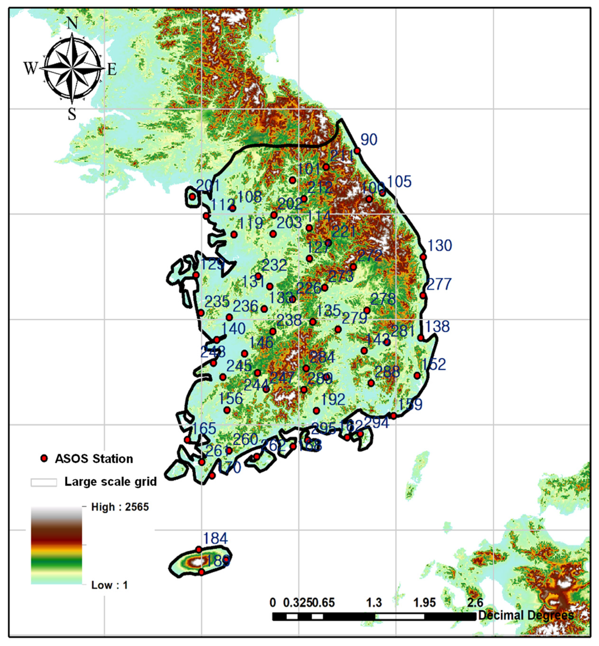
As shown in Figure 1, South Korea was selected as the study area. The large-scale reanalysis data were downscaled to the scale of the ground weather stations. The grid of reanalysis consisted of the 1.25° grids used by the Korea Meteorological Association (KMA) for global simulation, and 59 automated synoptic weather system (ASOS) stations were utilized as ground observation points. Figure 1 shows the ASOS stations, grids of reanalysis, and elevation. The annual average precipitation of the ASOS is approximately 1400 mm. The 18 grids cover most of South Korea.
2.2. Data Collection
The relationship between predictand and predictor used for spatial downscaling can be explored differently depending on the GCM performance for simulating predictand and predictor. Therefore, the relationship between predictor and predictand found in a specific GCM output may not be valid in other GCMs. To prevent this distortion in the results due to the different performances of various GCMs in terms of exploring the analog parameters, the perfect prognosis (PP) downscaling approach was adopted in this study [38]. In the PP approach, the relationship between the predictand (observed data) and the reliable predictors (e.g., reanalysis data) is derived, and this relationship is applied to the downscaling process. Since the relationship is not affected by the performance of the GCMs, it is reliable and applicable for downscaling all GCM outputs. Therefore, the PP approach is commonly used for the search parameters mentioned in the introduction section. However, its downscaling performance is relatively lower than that of other approaches because it does not consider model bias in the downscaling process.
In this study, reanalysis data were used as large-scale predictors, and the downscaling results were evaluated through comparisons with ground truth observed data. Table 1 shows the ground weather observations and reanalysis data collected in this study. To obtain ground observation data, daily precipitation data from 59 ASOS stations were collected over a 36-year period, and to obtain reanalysis data, reanalysis v5 (ERA5) data provided by the European Centre for Medium-Range Weather Forecasting (ECMWF) were collected over the same 36-year period. ERA5 data were upscaled from a 0.25° grid and hourly scale to a 1.25° grid and daily scale. The use of upscaled ERA5 data to search for the downscaling parameters was an efficient approach in terms of the associated computational costs [39]. Large-scale potential predictors, which are commonly used in previous studies, were selected [40]. The potential predictors consisted of circulation, thermal, and humidity variables known to be related to precipitation.
3. Methodology
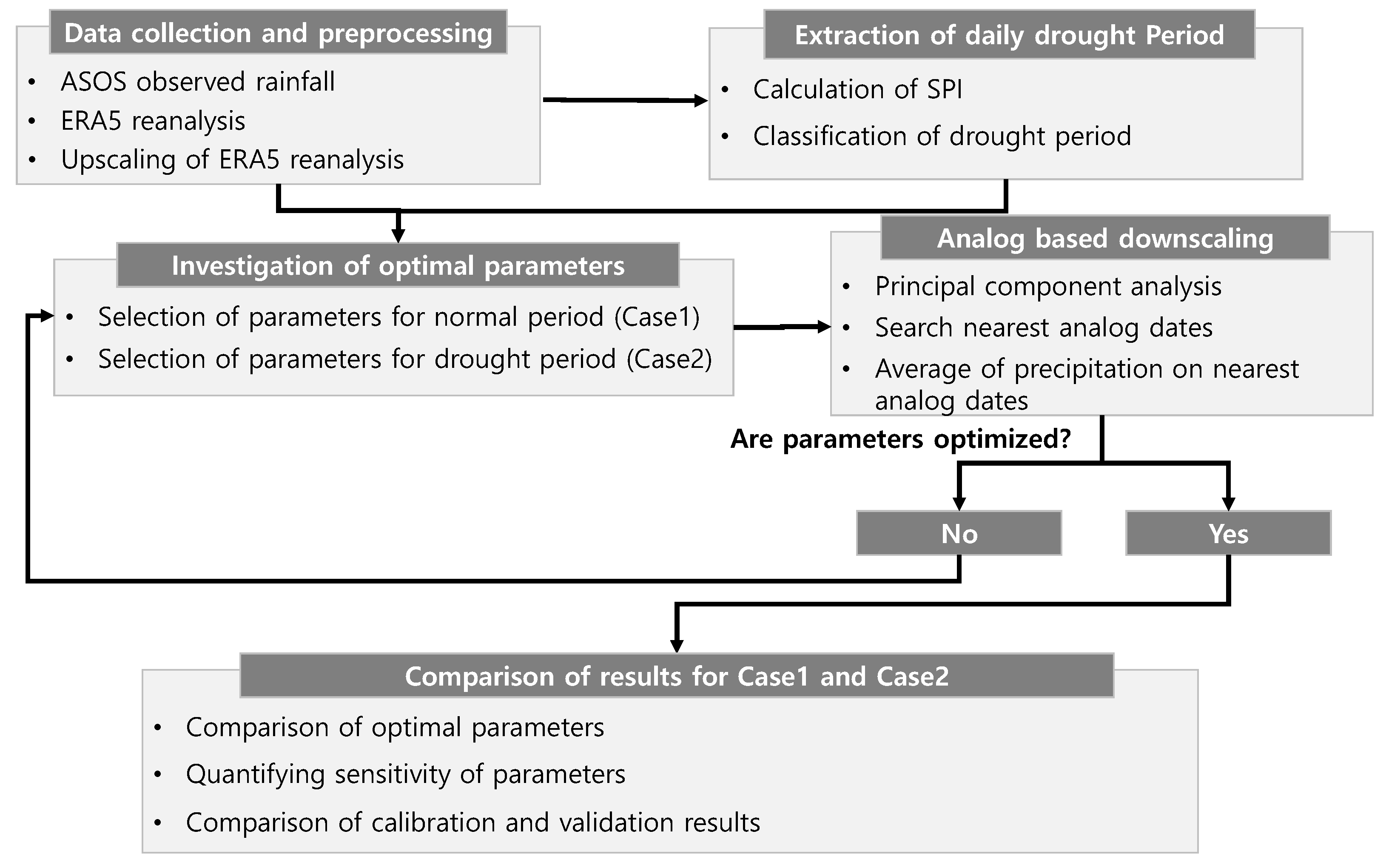
Figure 2 shows the methodological framework of this study. After collecting the data, daily drought periods were extracted by using the daily standardized precipitation index (SPI). Based on these drought periods, optimal parameter sets corresponding to the normal period (Case 1) and drought period (Case 2) were searched. Case 1 included flood, normal, and drought periods, while Case 2 included only drought periods. The performances of the downscaling results were evaluated and compared case by case. Finally, it was possible to derive the optimal parameter set and assess its sensitivity regarding the downscaling of daily precipitation in South Korea and to elaborate added values in the downscaling method to optimize the method for the drought period. All of these processes were implemented with MATLAB codes written by the authors.
3.1. Extraction of the Daily Drought Period
Seasonal or long-term precipitation is known to be related to very large-scale circulation features, such as the El Niño Southern Oscillation (ENSO) [33], while short-term precipitation is related to regional synoptic patterns. In this study, because we focused on short-term precipitation cases, regional synoptic patterns were considered. Because the downscaling method in this study was conducted at a daily scale, an index that is used to assess daily short-term drought was utilized. A daily SPI data series with a 28-day duration was adopted to extract the drought period. Series of drought indices are commonly adopted to assess short-term or very-short-term droughts, such as flash droughts [41,42]. The SPI was calculated based on the daily moving average of the precipitation data at all ASOS stations (Equations (1)–(5)). For each station, the corresponding drought period was constructed based on the dates when the SPI values were less than −1 (the criterion used to determine drought conditions) [43]:
where is the cumulative distribution function (CDF) based on the gamma distribution, is the 28-day cumulative precipitation, is a scale parameter, is a shape parameter, is the gamma function, and c0–c2 and d1–d3 are coefficients [43].
3.2. K-Nearest Analog Downscaling Method
Analog downscaling is performed with analog dates, which are extracted from historical dates. To prevent the analog downscaling performance from being artificially adjusted, the period for evaluating the downscaling performance and the period for extracting analog dates should be separated. In addition, for the calibration and validation of analog downscaling parameters, independent data periods are needed. In this study, the data period was divided into two periods (1980–1999 and 2000–2015). These two periods were then used as the validation and calibration periods. The analog parameter sets were obtained from the data corresponding to the calibration period and were used to verify the parameters for the validation period. When downscaling the calibration period, the analog dates were searched in the validation period. Downscaling the validation period, the analog dates were searched in calibration period.
In this work, the K-nearest-based approach was chosen as the downscaling method. This approach is one of simplest approaches for analog downscaling, and most analog-based downscaling methods are based on this type of simple structure [44,45,46]. Due to these characteristics, the K-nearest approach has been utilized to search for the parameters of the analog downscaling method rather than other sophisticated approaches [20]. The analog search process consisted of two steps. To consider seasonality, potential analog dates were preliminarily searched by using the average temperature similarities between the historical dates and target dates. After sorting the historical dates based on the average temperature similarities with the target dates, the dates with large similarity values were selected as potential analog dates. The number of potential analog dates (n1) was set to be equal to the length of a season (90 days) multiplied by the number of years in the calibration period. The analog dates used for the final downscaling process were selected from the potential analog dates by considering the similarities among the predictors. Hereafter, analog date size used for downscaling is called ‘K’ based on the K-nearest approach. To remove dependencies among predictors, a principal component analysis (PCA) was used. Principal component scores indicating normalized predictors with explanatory power greater than 80% were used to find the analog dates. The similarity of the scores between the target date and historical date was estimated using Euclidean distances (Equation (6)). Finally, the predictand (downscaled results) was calculated by averaging the local weather data across the K analog dates:
where is the station number, is the target date, is the historical date used in the analog search, is the number of principal scores, and is the lth principal score of the predictors.
3.3. Search of the Analog Parameter Sets
In this study, the predictor variables, domain size (hereafter D size), analog date size for downscaling (hereafter K size), and time dependency (hereafter T size) were explored as parameters in the analog downscaling method. The predictor variables included the large-scale atmospheric variables representing synoptic weather patterns that were utilized to find analog dates. Large-scale predictor variables should be physically linked to local-scale predictands and should also be accountable to local weather variabilities when used for downscaling. Most components that are physically related to rainfall are already known [38], but regionally relevant combinations of predictors and pressure levels must be explored. The D size refers to the appropriate spatial range that could reflect large-scale atmospheric states. This parameter is tightly linked to the selection of predictor variables. An appropriate D size contributes to the large-scale predictor being able to appropriately respond to local weather variations [20].
Analog methods are based on the assumption that historical meteorological phenomena will be reproduced in the future. However, in some cases, it is difficult to search for a meaningful analog date to the target date. In this case, the degradation of the downscaling performance is prevented by increasing the K size used in the downscaling process. Therefore, an appropriate K size is a significant parameter affecting the analog performance. The T size is mainly used for analog-based forecasting, and the temporal dependencies between predictors and predictands are considered by changing the time step of the predictor.
Because several parameters were explored in this work, a sequential methodology was adopted [24]. The parameter variables D size, K size and T size were searched in order. After all parameters were set to their default values, the parameters were optimized sequentially in the above order. To find the optimal predictor variable combination, a stepwise method was applied. In the process of the stepwise method, forward selection and backward elimination were applied iteratively to find the best combination of predictors. Although this approach has limitations in terms of considering all possible combinations, it has been widely used to select dependent variables in various areas due to its simplicity [38,47]. The values of the other parameters gradually increased, and the parameter value exhibiting the best downscaling performance was selected as the optimal parameter. The parameter sets were selected based on the downscaling performance of the daily precipitation data. The downscaling performance was evaluated based on the root mean square error (RMSE). The RMSE has been used as an objective function to search for parameters in previous studies [20,27]. This selection process was conducted for two cases. First, the downscaling performance in the normal period (Case 1) was considered; then, the downscaling performance of the drought period (Case 2) was assessed. Case 1 represents a conventional approach, while the approach applied to Case 2 attempted to derive parameter sets suitable for identifying drought conditions in this study.
4. Results
4.1. Extraction of the Daily Drought Period
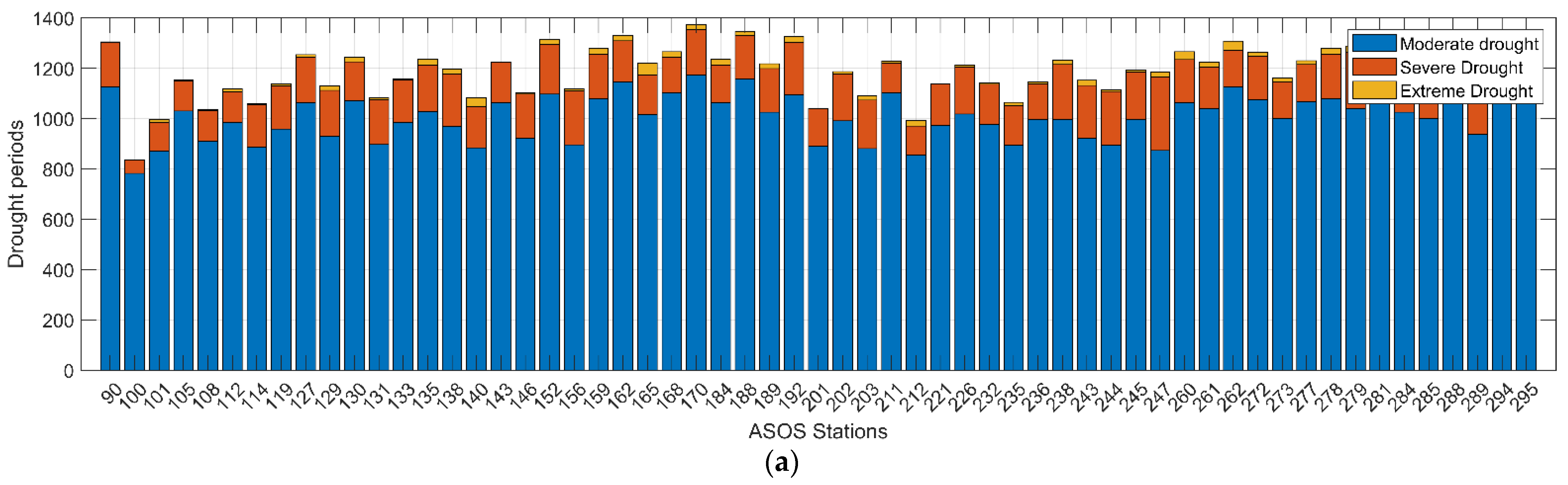
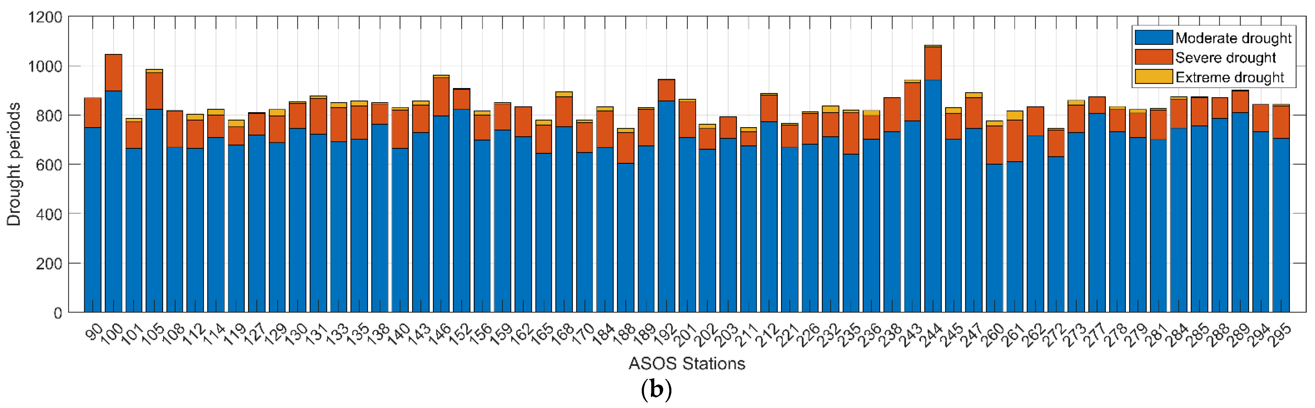
Figure 3 shows the results obtained by extracting the drought period from the ASOS station data. The drought period was extracted, and the severity values were classified based on the previously established drought classification criteria of the SPI by Mckee [43]. At most stations, approximately 14–17% of the analyzed period could be classified as reflecting drought conditions. This is an appropriate drought period proportion considering the SPI characteristics, as the SPI is calculated based on a standard Gaussian distribution.
4.2. Investigation of Optimal Predictor Variables
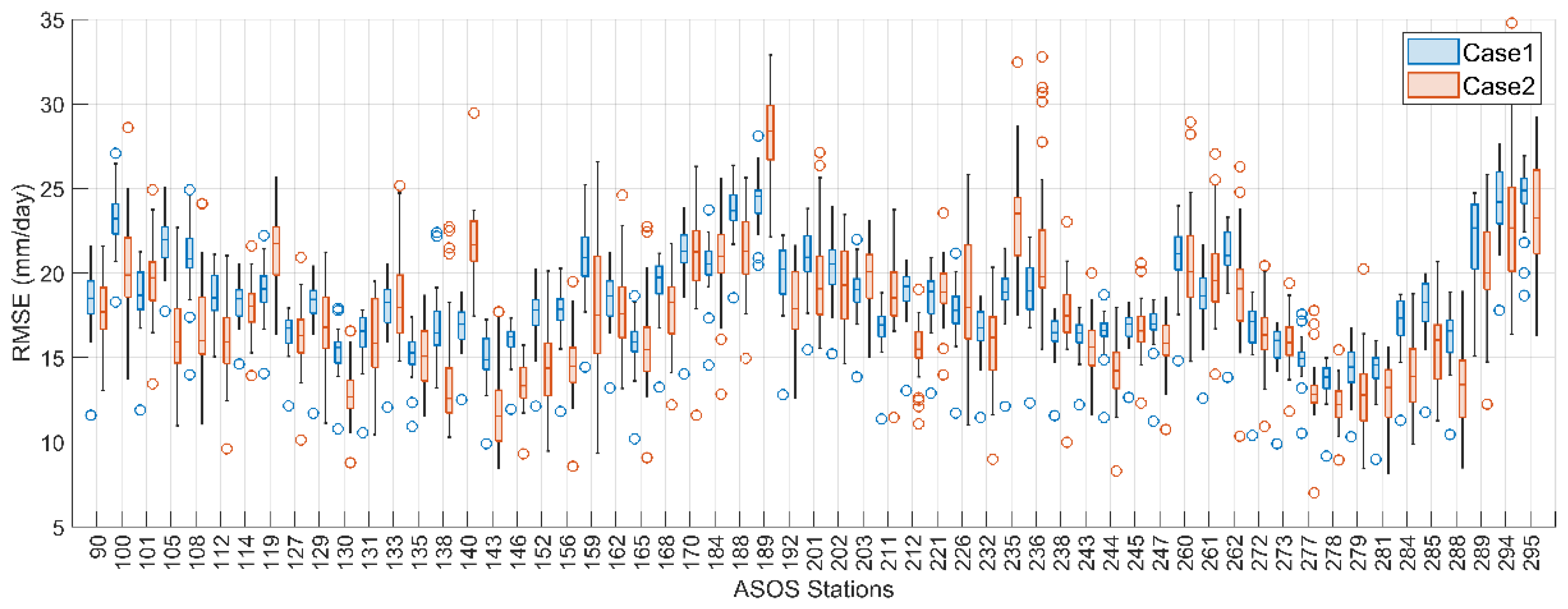
Figure 4 displays the results obtained after evaluating the downscaling performance based on a single predictor variable. The ranges of the box plots correspond to the RMSEs of the downscaled results based on each single predictor, as shown in Table 1. The average RMSE of Case 2 was slightly smaller than that of Case 1; the RMSE range of Case 2 was 38% greater than that of Case 1. This variation indicates that the drought period downscaling performance was more sensitive to the predictor selection than the performance obtained in normal periods. This result supports the concept stated herein that it is necessary to use parameters that are suitable for drought periods when attempting to downscale drought periods.
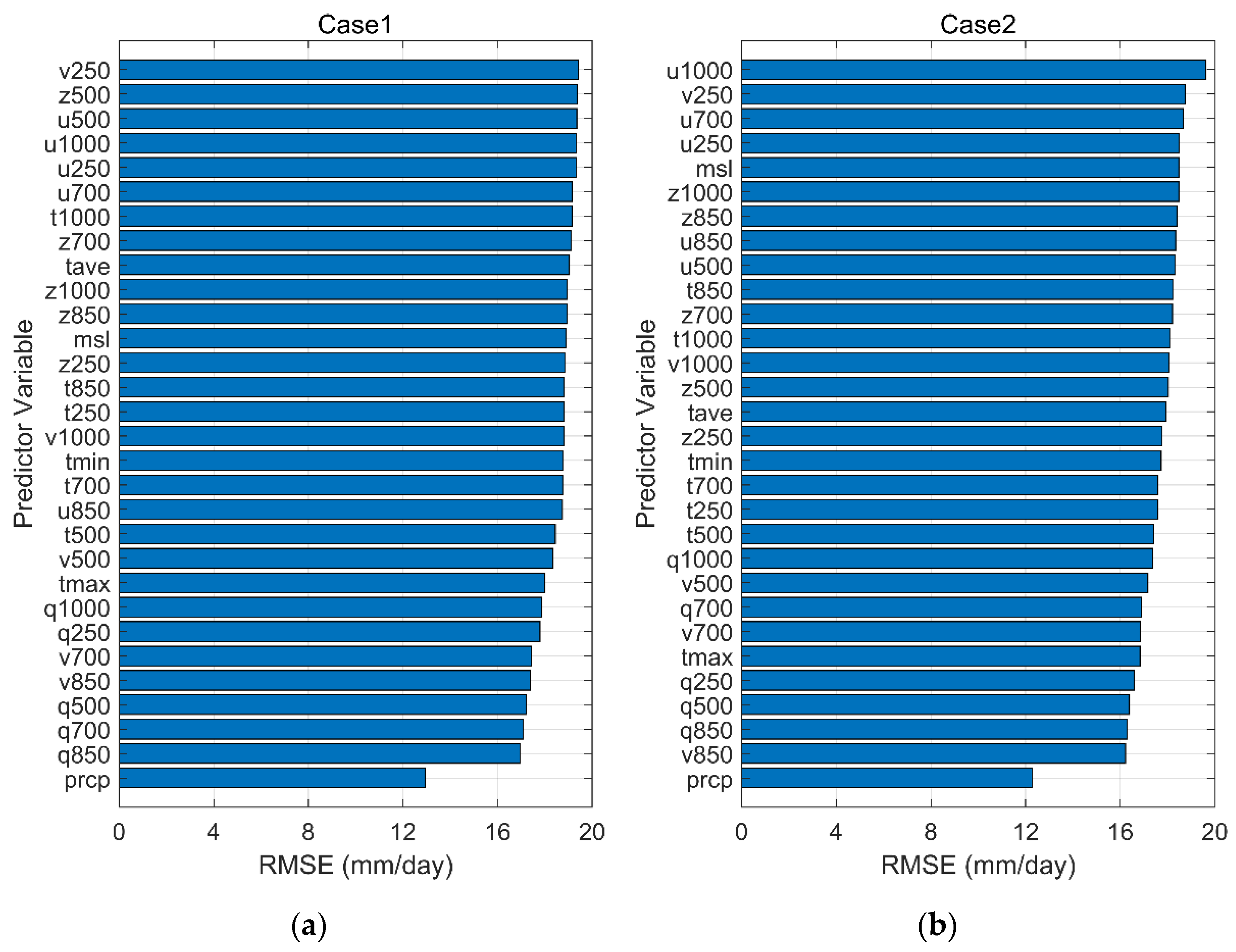
Figure 5 shows a comparison of the downscaling performance obtained for Case 1 and Case 2 using a single predictor. Each bar chart indicates the RMSE between the downscaling result and the observation based on each individual predictor. The results of both Case 1 and Case 2 showed that the maximum RMSE was approximately double the minimum RMSE. In other words, the predictor selection process was highly sensitive to the downscaling performance. In the Case 1 results, prcp showed the best performance for all stations. Additionally, v850, a circulation variable, and the humidity variables q850, q700, and q500 all showed high performances. The high-pressure-level variables showed lower RMSEs than the low-pressure-level variables. In Case 1 and Case 2, the top 10 predictors included similar variables, although their orders differed. In both cases, except for tmax, the performances of the thermal variables were low, while the performances of the humidity and circulation variables were comparatively high.
Previous literature has indicated that it is advantageous to use a combination of predictors rather than a single predictor in the downscaling process [20,21,27]. In this study, predictor combinations were searched for all stations, as shown in Table 2, through the stepwise method. When these combinations were used, the downscaling performance was 10.0% better than that obtained in the case in which individual predictors were used (Case 1) and 17.8% better than that in Case 2. The double combination was the most common, and the combination of prcp and circulation variables (u, v, z) was the most practical. Regarding the pressure level, the variables at 1000–700 mb showed relatively high performances.
By case, Case 1 and Case 2 had 41 stations for which different predictor variables were selected, composing approximately 70% of the total number of stations. To examine whether the optimal predictor set derived in Case 2 had added value compared to that in Case 1, the RMSEs obtained for Case 1 and Case 2 were compared during the drought period. Among the 41 stations where different predictors were selected between Case 1 and Case 2, the average RMSEs obtained for Case 2 were 10.5% smaller than the corresponding Case 1 RMSEs at 35 stations. Therefore, selecting drought period predictors can effectively improve the downscaled precipitation accuracy during a drought period. However, the lack of improvement at six stations was thought to be caused by the limitations of the stepwise method, as this method cannot consider all possible predictor combinations.
4.3. Investigation of Optimal D, K, and T Sizes
At each station, the optimal D size was searched for, and the shape of the domain was assumed to be a square. The search performance was evaluated by increasing the length of the side of the square by 2.5°. Nine cases were reviewed from a minimum of 1.25° to a maximum of 21.25°, and the optimal D size derived for each station is shown in Figure 6. In Case 1, more than 50% of the optimal D sizes were 1.25°, the minimum size. The D sizes were relatively large at the stations located in the southern coastal area. In South Korea, it is desirable to conduct downscaling using the smallest optimal D size at most stations, and in some southern coastal areas, D sizes of 3.75° to 6.25° should be adopted.
Comparing the results case by case, the D sizes obtained in Case 1 and Case 2 were similar. In Case 2, the minimum D size and D size of 3.75 were found at more stations, while the 6.25 D size was optimal for fewer stations. The average domain sizes were 4.09° for Case 1 and 3.62° for Case 2. Thus, the optimal D size was slightly smaller in the drought case than in the normal case.
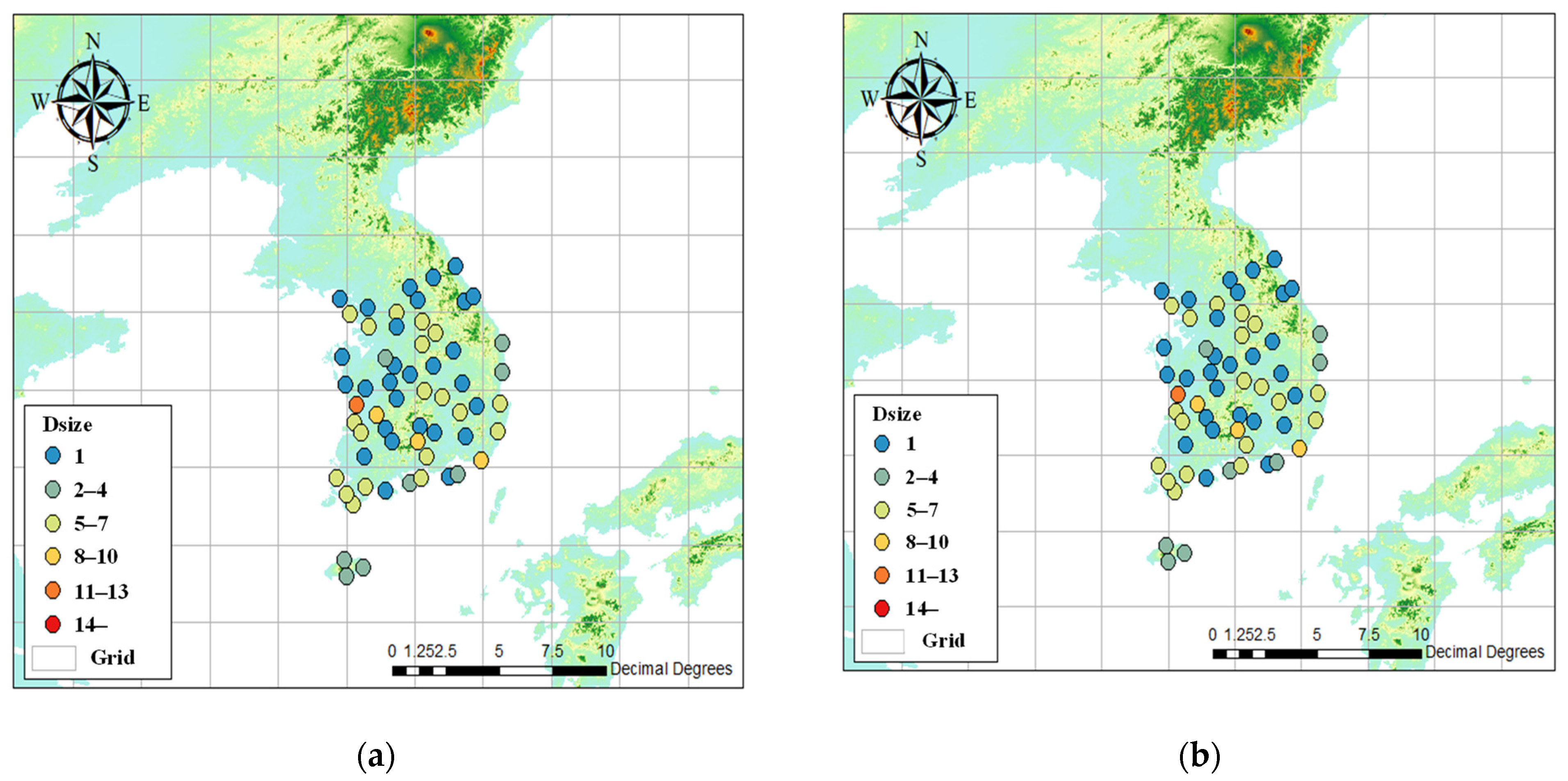
Figure 7 indicates the optimal K size for the ASOS stations. Each optimal K size was selected as the value that resulted in the best downscaling performance as K was increased from 1 to 41 by 2. The average optimal K obtained in Case 1 was 13.38, and the optimal Ks of inland stations were larger than the optimal Ks at coastal stations. The optimal K sizes were mostly distributed between 5 and 13, and stations with relatively large K sizes were distributed in western South Korea. The optimal K value obtained in Case 2 was 12.3% larger than that derived in Case 1. Unlike Case 1, in which the optimal Ks were large only at inland stations, in Case 2, the optimal Ks were relatively large at most stations. Because it is difficult to find a small number of informative analog dates that are suitable for representing unusual drought conditions, it was likely that the optimal K values obtained in Case 2 would be larger than those of Case 1. As shown in Figure 7, the appropriate K value may differ between drought and normal periods. These results support the idea of this study that suitable parameters should be explored for drought periods when performing drought assessments.
In this study, the time dependency (T size) was also searched for case by case. The predictors were averaged depending on the T size and subsequently adopted for the downscaling process. Each optimal T size was selected as the value with the best downscaling performance as T was increased from 1 to 31 by 2. In both cases, 1 was selected as the optimal T value. As the T size increased, the downscaling performance decreased at all stations, indicating that the synoptic predictor before the target date had no valid relationship with the predictand. Therefore, it was not necessary to consider the time dependence parameter when performing downscaling research rather than forecasting research.
4.4. Sensitivity of Parameters
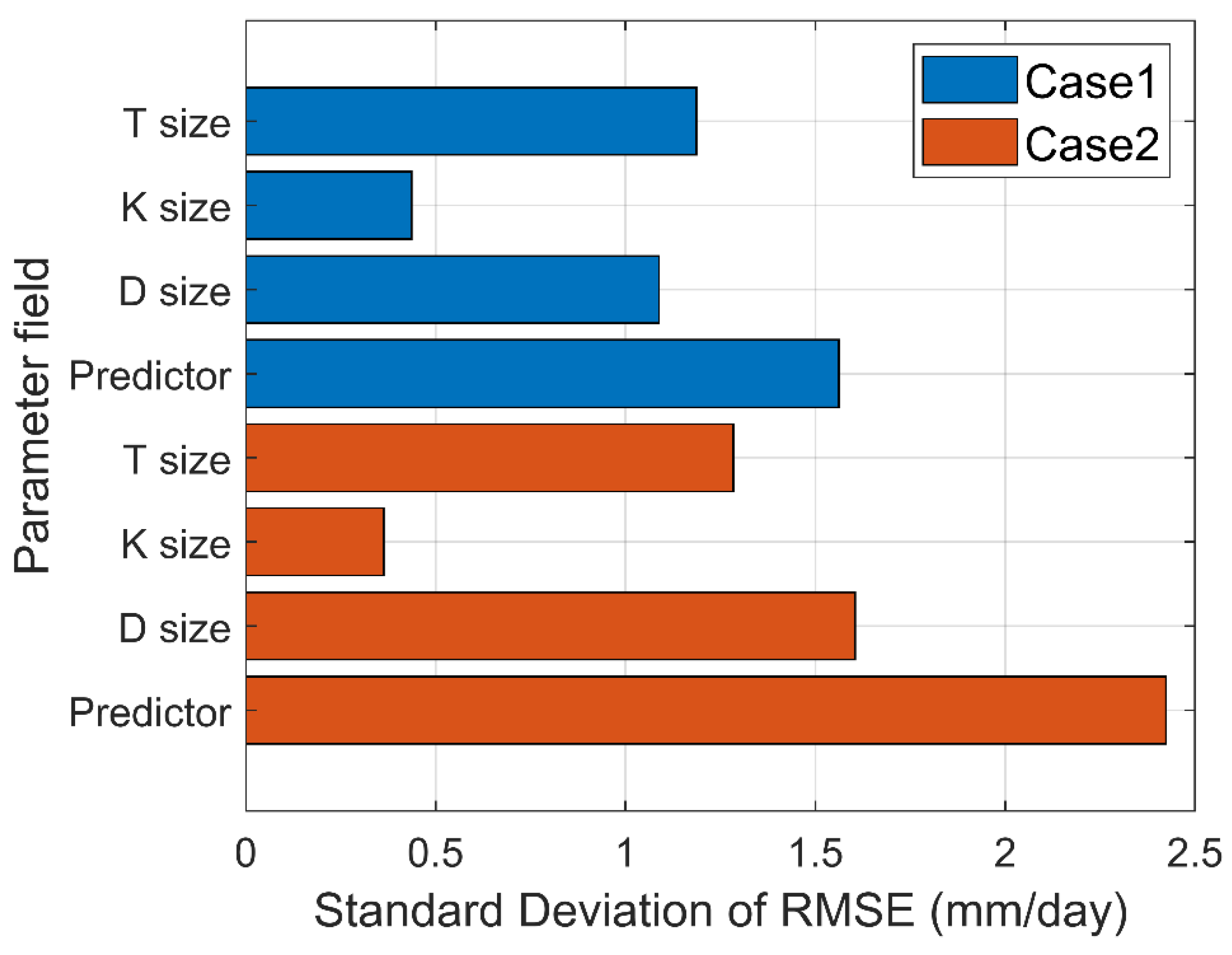
Figure 8 shows the sensitivity of each parameter, as assessed by comparing the parameter changes to the downscaling performances. The sensitivities were evaluated using the standard deviation of the RMSE. The larger the standard deviation was, the greater the sensitivity was. The standard deviation values of the T size and K size indicated RMSE changes when each parameter changed by 2. The standard deviation value of the D size indicated an RMSE change when the D size increased by 2.5°, and the predictors were assessed using the RMSE changes in accordance with the changes in the 30 individual predictors. Because each parameter had different characteristics, it was difficult to compare these sensitivities directly. However, these results can be informative due to the lack of similar references in South Korea.
As a result of the sensitivity tests performed for Case 1, the predictor variable was found to be the most sensitive parameter in the downscaling process, with a standard deviation of 1.56. In addition, the T size, D size, and K size were sensitive to the downscaling performance. Because the T size was not an effective parameter for downscaling, it could be ignored in the sensitivity results. Comparing Case 1 and Case 2, the Case 2 parameter sensitivity levels were greater than the Case 1 sensitivities. The sensitivities of the predictor variable and D size in Case 2 were 55% and 47% higher than those in Case 1, respectively, and the sensitivity of the K size showed no significant difference between the two cases, suggesting that the parameter optimization process is more important when conducting spatial downscaling for drought periods than for normal periods.
4.5. Comparison of the Calibration and Validation Sets
The results described in Section 4.2, Section 4.3 and Section 4.4 are the results of the analog downscaling parameter search based on the calibration set. In the current section, the robustness of the searched parameters was reviewed by comparing the downscaling results obtained during the calibration and validation periods. The calibration results were calculated based on the downscaling period (2000–2015) and the analog search period (1980–1999). The validation results were calculated based on the downscaling period (1980–1999) and analog search period (2000–2015).
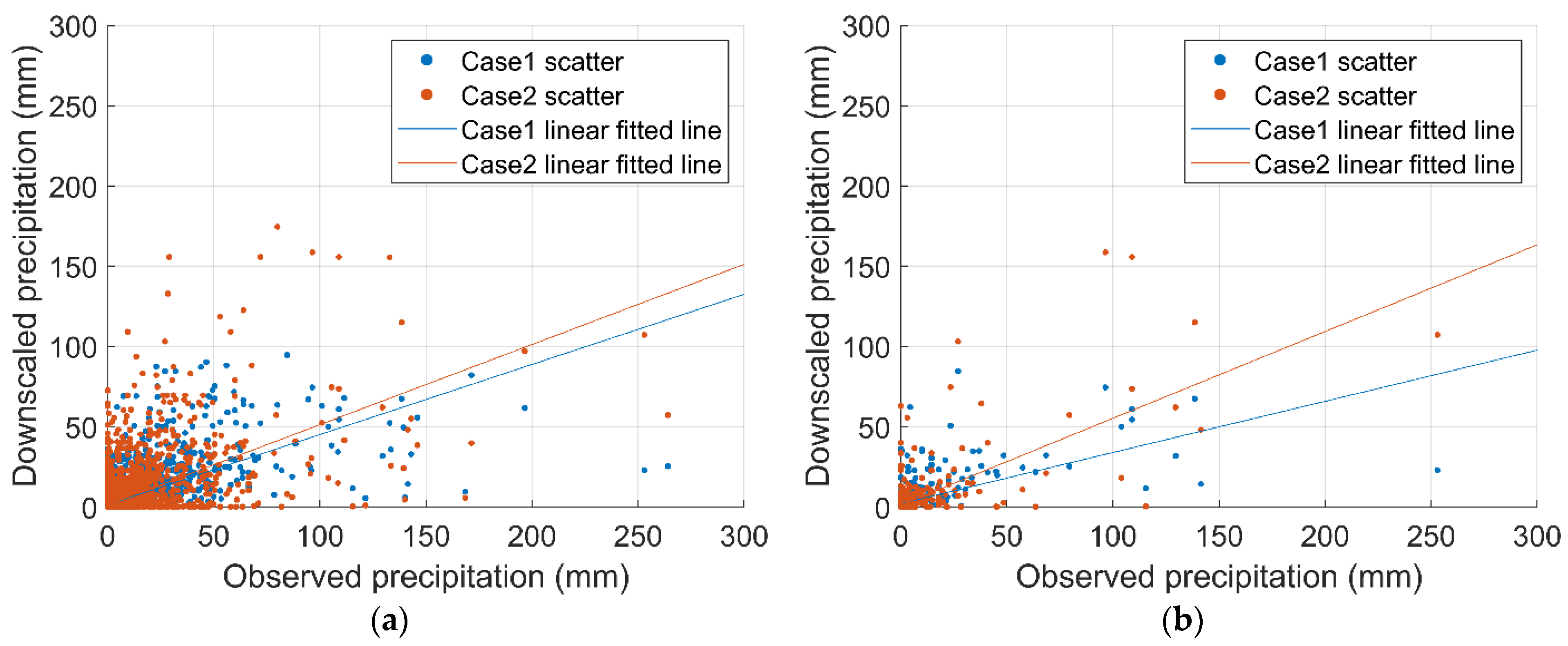
Figure 9 shows a scatter plot between the observation and downscaling results obtained during the calibration period of station 235. For both the normal and drought periods, the downscaling results were lower than the observations. The lower results were due to the bias of the ERA5 reanalysis. Since no bias correction function was contained in the PP downscaling process, the downscaling results were also lower. In most normal periods, the results of Case 1 and Case 2 were similar. However, the results of Case 2 were significantly different from the observations for a few days. In the drought period, the results of Case 2 were closer to the observations than the results of Case 1. Therefore, it was confirmed that Case 1 was relatively effective in the normal period and that Case 2 was effective in the drought period.
Table 3 shows the calibration and validation metrics achieved for Case 1 and Case 2. As the Case 1 results reveal, no significant difference was found in the downscaling performances between the calibration and validation periods; this result supported the concept that the searched parameter set was robust. On the other hand, in the Case 2 results, a relatively large difference could be observed between the calibration and validation results. Therefore, the Case 2 parameters were comparatively less stable than the Case 1 parameters.
To review whether the downscaling parameters suitable for the drought period had added value, the downscaled results based on the optimized parameter sets obtained for Case 1 and Case 2 were compared in the drought period. As a result of comparing the Case 1 and Case 2 parameter sets, the same parameter was searched for at three stations, and different parameters were searched for at 56 stations. During the calibration period, the Case 2 results reflected average RMSEs that were 8.2% (range: 1.3–28.4%) smaller than the corresponding RMSEs obtained under Case 1 at 39 stations. During the validation period, the Case 2 results reflected average RMSEs that were 6.3% (range: 1.2–25.4%) smaller than those of Case 1 at 23 stations. In the calibration period, the drought period-suitable parameters were shown to be effective for most stations. Although the number of effective stations decreased during the validation period, these parameters were still effective for a significant number of stations.
5. Discussion
In this study, the optimal parameters and parameter sensitivities associated with the analog downscaling process were explored for South Korea, and the added value provided by the optimal parameters for the drought period was reviewed. In this section, we discuss the results and limitations of this work, as well as future research ideas.
To review the usefulness of the searched parameters, the parameters for the normal period were compared with the results of previous studies. Regarding the predictor variables, previous studies have indicated that it is advantageous to use a combination of predictors rather than a single predictor in the downscaling process [20,21,27]. Several previous studies have also suggested that prcp, which is estimated by climate models, is among the best predictors for downscaling precipitation [13,27,40,48], and they showed that the use of circulation variables can improve precipitation downscaling results [29]. These results are consistent with the results of this research. However, some studies have mentioned that msl, z850, z500, and t850 are informative for the downscaling approach [29,49], but in this study, the performances of these predictors were relatively low compared to the other predictors. This was because the predictors that were not reviewed in previous research achieved better performances than these suggested predictors.
For D size, previous studies have revealed that small domains are advantageous for downscaling, and due to the influence of the ocean, the D sizes of the stations in these coastal regions are larger than those of the stations in inland regions [25,27]. These studies presented characteristics that were similar to those of the results of this research. For K size, in previous studies, the appropriate K was 30 considering the size of sample data and the number of degrees of freedom [16], but according to the results presented in this study, effective performance was achieved at a relatively low K. This may have been caused by the use of different downscaling methods. The downscaling method in this study was a simple averaging approach rather than a regression technique. T size is not an effective parameter for downscaling daily precipitation, and previous research also mentioned that T size is mostly effective for long-term downscaling or forecasting research rather than daily downscaling [50]. Since most of the parameters explored in this study were consistent with those of previous studies, this inference is reasonable. Therefore, it is concluded that the suggested parameters in the normal period are informative in the application of analog and other downscaling approaches in South Korea.
Several aspects must be improved regarding the search for downscaling parameters due to the lack of related research conducted in South Korea. In this study, a sequential methodology was adopted to search for downscaling parameters, and this methodology could not consider combinational effects among parameters. The sequential results were thus discussed as semi-optimized parameters [39], and a global optimization methodology was proposed to conduct complete optimization. Since the global optimization methodology consumes vast computational resources, there are few applied cases, but this direction should be considered in the future. Additionally, the searched parameter set is expected to differ depending on the selected reanalysis product [39,51]. In this study, ERA5, one of most advanced reanalysis datasets available [39,52], was applied, but it is necessary to examine how the parameter search results would be affected by the use of other reanalysis data. Lastly, although the parameter sensitivity and quantitative values are presented in this study, the characteristics of the increase, decrease, or bias of the downscaling results according to each parameter were not analyzed in detail. Further detailed follow-up studies are needed to improve the parameter search. It is also necessary to consider a decision tree-based methodology, which can be a powerful tool for such detailed studies [53,54,55].
The search parameters for the drought period exhibited advantages in the downscaling process for the drought period. However, the stability of the parameters was relatively low, and to apply the parameters that were suitable for the drought period to downscaling, it is necessary to improve the stability of the parameters. In this study, the drought period was classified by using only the amount of precipitation. This simple drought classification methodology may not be sensitive to the holistic extraction of drought periods, which have valid relationships with other large-scale predictors. It is not difficult to find studies that have attempted to analyze the synoptic weather patterns associated with drought occurrences [35,36,37]. Therefore, if drought classifications are conducted based not only on precipitation but also on these synoptic weather patterns, drought periods that are highly correlated with synoptic weather patterns can be derived. This sensitive drought classification process could improve the stability of the downscaling parameters used to represent drought conditions.
In addition, to derive more stable drought period parameters, it is necessary to apply a seasonal parameter extraction methodology. Because South Korea is dominated by the Asian monsoon climate and experiences large monthly precipitation variations, the rainfall mechanisms in this region differ substantially from season to season. Therefore, if a single parameter is derived without considering these mechanisms, the stability of the resulting parameters may be poor. Thus, methodologies in which seasonal effects are considered must be applied to both normal and drought periods.
6. Conclusions
In this study, optimal parameter sets, that are suitable for the downscaling of daily precipitation in the cases of normal and drought periods in South Korea, were presented, and the added value of considering the optimal drought period parameters was elaborated.
As a summary of the parameter search results for the normal period, the sensitivities of the parameters to the downscaling performance were large in the following order: the predictor variables, D size, and K size. The combination of predictor variables was more advantageous than a single predictor. The combination of prcp and the circulation variables yielded the best performance. For D size, the smallest grid was advantageous for downscaling, and a relatively large D size was effective for the southwest coast of South Korea. The average K size was 13.38, and T size was meaningless with respect to downscaling performance. The normal period parameters were reasonably calculated due to their relatively high stability and their consistency across other studies. This result is valuable because it can provide a reference not only for analog downscaling but also for other downscaling methods for South Korea.
As a summary of the parameter search results in the drought period, the order of the parameters in terms of sensitivity was similar to that of the normal case. However, the parameters were much more sensitive than in the normal case. For the predictor variables, as in the normal case, the combination of prcp and the circulation variables yielded high downscaling performance, but the selected variables were different from those used in the normal case at 70% of the stations. For D size, the smallest grid was also effective for downscaling, and the average K size was 12.3% larger than that in the normal case. T size was also not effective for the downscaling of daily precipitation. To examine the added value provided by the drought period parameters, the performances of the normal parameters and the drought parameters were compared for the drought period. The downscaling performance achieved based on the drought parameters was better than that yielded based on the normal parameters at most stations. It is concluded that suitable drought parameters provide added value in the downscaling process.
This study was meaningful in that it provided downscaling parameter information with high usability with regard to the South Korean region, where climate change and spatial downscaling studies are being actively conducted [5,13,53]. In addition, this study represents a scientific contribution in that it presents a new perspective for achieving improved downscaling performance for drought periods by considering drought conditions when searching for downscaling parameters. In the future, more downscaling approach studies considering these conditions are expected to be conducted to improve the overall downscaling performance.
Author Contributions
Conceptualization, S.-H.K.; methodology, S.-H.K.; software, S.-H.K.; validation, S.-H.K.; formal analysis, S.-H.K.; investigation, J.-B.K.; resources, J.-B.K.; data curation, J.-B.K.; writing—original draft preparation, S.-H.K.; writing—review and editing, S.-H.K.; visualization, J.-B.K.; supervision, D.-H.B.; project administration, D.-H.B.; funding acquisition, D.-H.B. All authors have read and agreed to the published version of the manuscript.
Funding
This work was supported by the faculty research fund of Sejong University in 2021 (no. 20210595).
Institutional Review Board Statement
Not applicable.
Informed Consent Statement
Not applicable.
Data Availability Statement
The data used in this study were collected from the Korea Meteorological Association and the European Centre for Medium-range Weather Forecasting at https://data.kma.go.kr/cmmn/main.do, (accessed on 8 February 2022) and https://cds.climate.copernicus.eu/cdsapp#!/dataset/reanalysis-era5-pressure-levels?tab=overview (accessed on 15 September 2020).
Acknowledgments
We thank the two anonymous reviewers for their valuable comments and constructive suggestions regarding this manuscript.
Conflicts of Interest
The authors declare no conflict of interest.
References
- Kossin, J.P.; Hall, T.; Knutson, T.; Kunkel, K.E.; Trapp, R.J.; Waliser, D.E.; Wehner, M.F. Chapter 9: Extreme Storms. In Climate Science Special Report; U.S. Department of Commerce: Lincoln, NE, USA, 2017. [Google Scholar]
- Masson-Delmotte, V.; Zhai, P.; Pörtner, H.O.; Roberts, D.; Skea, J.; Shukla, P.R.; Pirani, A.; Moufouma-Okia, W.; Péan, C.; Pidcock, R.; et al. Global Warming of 1.5 °C; IPCC Special Report; IPCC: Geneva, Switzerland, 2018. [Google Scholar]
- Pörtner, H.O.; Roberts, D.C.; Masson-Delmotte, V.; Zhai, P.; Tignor, M.; Poloczanska, E.; Mintenbeck, K.; Alegría, A.; Nicolai, M.; Okem, A.; et al. Special Report on the Ocean and Cryosphere in a Changing Climate; IPCC Special Report; IPCC: Geneva, Switzerland, 2019. [Google Scholar]
- Bae, D.H.; Koike, T.; Awan, J.A.; Lee, M.H.; Son, K.H. Climate change impacts assessment on water resources and susceptible zones identification in Asian Monsson region. Water Resour. Manag. 2015, 29, 5377–5393. [Google Scholar] [CrossRef]
- Lee, M.H.; Im, E.S.; Bae, D.H. Impact of spatial variability of daily precipitation on hydrological projection: A Comparison of GCM- and RCM-driven Cases in the Han River basin, Korea. Hydrol. Process 2019, 13, 2240–2257. [Google Scholar] [CrossRef]
- Kim, J.B.; Im, E.S.; Bae, D.H. Intensified hydroclimate response in Korea under 1.5 and 2 °C global warming. Int. J. Climatol. 2020, 40, 1965–1978. [Google Scholar] [CrossRef]
- Gangopadhyay, S.; Clark, M.; Rajagopalan, B. Statistical downscaling using K-nearnest neighbors. Water Resour. Res. 2005, 41, W02024. [Google Scholar] [CrossRef] [Green Version]
- Fowler, H.J.; Blenkinsop, S.; Tebaldi, C. Linking climate change modelling to impacts studies: Recent advances in downscaling techniques for hydrological modelling. Int. J. Climatol. 2007, 27, 1547–1578. [Google Scholar] [CrossRef]
- Wootten, A.M.; Massoud, E.C.; Sengupta, A.; Waliser, D.E.; Lee, H. The Effect of Statistical Downscaling on the Weighting of Multi-Model Ensembles of Precipitation. Climate 2020, 8, 138. [Google Scholar] [CrossRef]
- Wilby, R.L.; Wigley, T.M.L. Downscaling general circulation model output: A review of methods and limitations. Prog. Phys. Geog. 1997, 21, 530–548. [Google Scholar] [CrossRef]
- Maraun, D.; Widmann, M.; Gutiérrez, J.M.; Kotlarski, S.; Chandler, R.E.; Hertig, E.; Wibig, J.; Huth, R.; Wilcke, R.A.I. VALUE: A framework to validate downscaling approaches for climate change studies. Earth’s Future 2015, 3, 1–14. [Google Scholar] [CrossRef] [Green Version]
- Maraun, D. Bias Correcting Climate Change Simulations—A Critical Review. Curr. Clim. Change Rep. 2016, 2, 211–220. [Google Scholar] [CrossRef] [Green Version]
- Eum, H.I.; Cannon, A.J.; Murdock, T.Q. Intercomparison of multiple statistical downscaling methods: Multi-criteria model selection for South Korea. Stoch. Environ. Res. Risk Assess. 2016, 31, 683–703. [Google Scholar] [CrossRef]
- Wang, G.; Kirchhoff, C.; Seth, A.; Abatzoglou, J.T.; Livneh, B.; Pierce, D.W.; Fomenko, L.; Ding, T. Projected Changes of Precipitation Characteristics Depend on Downscaling Method and Training Data: MACA versus LOCA Using the US Northeast as an Example. J. Hydrometeorol. 2020, 21, 2739–2758. [Google Scholar] [CrossRef]
- Zhang, X.; Shen, M.; Chen, J.; Homan, J.W.; Busteed, P.R. Evaluation of Statistical Downscaling Methods for Simulating Daily Precipitation Distribution, Frequency, and Temporal Sequence. Trans. ASABE 2021, 64, 771–784. [Google Scholar] [CrossRef]
- Hidalgo, H.G.; Dettinger, M.D.; Cayan, D.R. Downscaling with Constructed Analogues: Daily Precipitation and Temperature Fields over the United States; California Energy Commission Report; California Energy Comission: Sacramento, CA, USA, 2008.
- Pierce, D.W.; Cayan, D.R.; Thrasher, B.L. Statistical Downscaling Using Localized Constructed Analogs (LOCA). J. Hydrometeorol. 2014, 15, 2558–2585. [Google Scholar] [CrossRef]
- Zorita, E.; von Storch, H. The analog method as a simple statistical downscaling technique: Comparison with more complicated methods. J. Clim. 1999, 12, 2474–2489. [Google Scholar] [CrossRef]
- Maurer, E.P.; Hidalgo, H.G. Utility of daily vs. monthly large-scale climate data: An intercomparison of two statistical downscaling methods. Hydrol. Earth Syst. Sci. 2008, 12, 551–563. [Google Scholar] [CrossRef] [Green Version]
- Bettolli, M.L.; Penalba, O.C. Statistical downscaling of daily precipitation and temperatures in southern La Plata Basin. Int. J. Climatol. 2018, 38, 3705–3722. [Google Scholar] [CrossRef]
- Chardon, J.; Hingray, B.; Favre, A.C. An adaptive two-stage analog/regression model for probabilistic prediction of small-scale precipitation in France. Hydrol. Earth Syst. Sci. 2018, 22, 265–286. [Google Scholar] [CrossRef] [Green Version]
- Bettolli, M.L. Analog models empirical-statistical downscaling. Clim. Sci. 2021, 23, 1–25. [Google Scholar]
- Timbal, B.; McAvaney, B.J. An analogue-based method to downscale surface air temperature: Application for Australia. Clim. Dyn. 2001, 17, 947–963. [Google Scholar] [CrossRef]
- Radanovics, S.; Vidal, J.P.; Sauquet, E.; Ben Daoud, A.B.; Bontron, G. Optimising predictor domains for spatially coherent precipitation downscaling. Hydrol. Earth Syst. Sci. 2013, 17, 4189–4208. [Google Scholar] [CrossRef] [Green Version]
- Chardon, J.; Hingray, B.; Favre, A.C.; Autin, P.; Gailhard, J. Spatial similarity and transferability of analog dates for precipitation downscaling over France. J. Clim. 2014, 27, 5051–5074. [Google Scholar] [CrossRef]
- Horton, P.; Jaboyedoff, M.; Obled, C. Global optimization of an analog method by means of genetic algorithms. Mon. Weather Rev. 2017, 145, 1275–1294. [Google Scholar] [CrossRef] [Green Version]
- Akhter, J.; Das, L.; Meher, J.K.; Deb, A. Evaluation of different large-scale predictor-based statistical downscaling models in simulating zone-wise monsoon precipitation over India. Int. J. Climatol. 2017, 39, 465–482. [Google Scholar] [CrossRef] [Green Version]
- Pour, S.H.; Harun, S.B.; Shahid, S. Genetic programming for the downscaling of extreme rainfall events on the east coast of Peninsular Malaysia. Atmosphere 2014, 5, 914–936. [Google Scholar] [CrossRef] [Green Version]
- Kang, H.; Park, C.K.; Hameed, S.N.; Ashok, K. Statistical downscaling precipitation in Korea using multimodel output variables as predictors. Mon. Weather Rev. 2009, 137, 1928–1938. [Google Scholar] [CrossRef]
- Kang, S.; Hur, J.; Ahn, J.B. Statistical downscaling method based on APCC multi-model ensemble for seasonal prediction over South Korea. Int. J. Climatol. 2014, 34, 3801–3810. [Google Scholar] [CrossRef]
- Ghafouri-Azar, M.; Bae, D.H. Analyzing the Variability in Low-Flow projections under GCM CMIP5-Scenarios. Water Resour. Manag. 2019, 33, 5035–5050. [Google Scholar] [CrossRef]
- Kim, J.B.; So, J.M.; Bae, D.H. Global Warming Impacts on Severe Drought Characteristics in Asia Monsoon Region. Water 2020, 12, 1360. [Google Scholar] [CrossRef]
- Hao, Z.; Singh, V.P.; Xia, Y. Seasonal Drought Prediction: Advances, Challenges, and Future Prospects. Rev. Geophys. 2018, 56, 108–141. [Google Scholar] [CrossRef] [Green Version]
- Kuswanto, H.; Yuliantin, I.L.; Khoiri, H. Statistical downscaling to predict drought events using high resolution satellite based geopotential data. In IOP Conference Series: Materials Science and Engineering; IOP Publishing: Bristol, UK, 2019; Volume 546, p. 052040. [Google Scholar]
- Yang, J.S. Synoptic climatological characteristics of spring droughts in Korea. J. Korean Assoc. Reg. Geogr. 1998, 4, 43–56. [Google Scholar]
- Yang, J.S. Synoptic climatological characteristics of autumn drought in Korea. J. Korean Assoc. Reg. Geogr. 2000, 6, 57–69. [Google Scholar]
- Yang, J.S. Synoptic climatological characteristics of winter drought in Korea. J. Korean Assoc. Reg. Geogr. 2005, 11, 429–439. [Google Scholar]
- Gutiérrez, J.M.; Maraun, D.; Widmann, M.; Huth, R.; Hertig, E.; Benestad, R.; Roessler, O.; Wibig, J.; Wilcke, R.; Kotlarski, S.; et al. An Intercomparison of a large ensemble of statistical downscaling methods over Europe: Results from the VALUE perfect predictior cross-validation experiment. Int. J. Climatol. 2019, 39, 3750–3785. [Google Scholar] [CrossRef]
- Horton, P. Analogue methods and ERA5: Benefits and pitfalls. Int. J. Climatol. 2021, 1–19. [Google Scholar] [CrossRef]
- Lu, E.; Zeng, X.; Jiang, Z.; Wang, Y.; Zhang, Q. Precipitation and precipitable water: Their temporal-spatial behaviors and use in determining monsoon onset/retreat and monsoon regions. J. Geophys. Res. 2009, 114, 105. [Google Scholar] [CrossRef] [Green Version]
- Parker, T.; Gallant, A.; Hobbins, M.; Hoggmann, D. Flash drought in Australia and its relationship to evaporative demand. Environ. Res. Lett. 2021, 16, 064033. [Google Scholar] [CrossRef]
- Noguera, I.; Domínguez-Castro, F.; Vicente-Serrano, S.M. Flash Drought Response to Precipitation and Atmospheric Evaporative Demand in Spain. Atmosphere 2021, 12, 165. [Google Scholar] [CrossRef]
- McKee, T.B.; Doesken, N.J.; Kleist, J. Drought monitoring with multiple time scales. In Proceedings of the 9th Conference on Applied Climatology, Dallas, TX, USA, 15–20 January 1995; pp. 233–236. [Google Scholar]
- Gutiérrez, J.M.; San Martín, D.; Brands, S.; Manzanas, R.; Herrera, S. Reassessing statistical downscaling techniques for their robust application under climate change conditions. J. Clim. 2013, 26, 171–188. [Google Scholar] [CrossRef] [Green Version]
- San-Martín, D.; Manzanas, R.; Brands, S.; Herrera, S.; Gutiérrez, J.M. Reassessing model undcertainty for regional proejctions of precipitation with an ensemble of statistical downscaling methods. J. Clim. 2017, 30, 203–223. [Google Scholar] [CrossRef]
- Fernández, J.; Saenz, J. Improved field reconstruction with the analog method: Searching the CCA space. Clim. Res. 2013, 24, 199–213. [Google Scholar] [CrossRef]
- Bedia, J.; Baño-Medina, J.; Legasa, M.N.; Iturbide, M.; Manzanas, R.; Herrera, S.; Casanueva, A.; San-Martín, D.; Confiño, A.S.; Gutiérrez, J.M. Statistical downscaling with the downscaleR package: Contribution to the VALUE intercomparison experiment. Geosci. Model Dev. 2020, 13, 1711–1735. [Google Scholar] [CrossRef] [Green Version]
- Keum, W.; Lim, G.H. Correlation between total precipitable water and precipitation over East Asia. In Geophysical Research Abstracts; Copernicus Publications: Göttingen, Germany, 2017; Volume 19, p. 8131. [Google Scholar]
- Min, Y.M.; Kryjov, V.N.; Oh, J.H. Probabilistic interpretation of regression-based downscaled seasonal ensemble predictions with the estimation of uncertainty. J. Geophys. Res. Atmos. 2011, 116, D08101. [Google Scholar] [CrossRef] [Green Version]
- Matulla, C.; Zhang, X.; Wang, X.L.; Wang, J.; Zorita, E.; Wanger, S.; von Storch, H. Influence of similarity measures on the performance of the analog method for downscaling daily precipitation. Clim. Dyn. 2008, 30, 133–144. [Google Scholar] [CrossRef]
- Horton, P.; Brönnimann, S. Impact of global atmospheric reanalyses on statistical precipitation downscaling. Clim. Dyn. 2019, 52, 5189–5211. [Google Scholar] [CrossRef]
- Hersbach, H.; Bell, B.; Berrisford, P.; Hirahara, S.; Horanyi, A.; Muñoz-Sabater, J.; Nicolas, J.; Peubey, C.; Radu, R.; Schepers, D.; et al. The ERA5 global reanalysis. Q. J. R. Meteorol. Soc. 2020, 146, 1999–2049. [Google Scholar] [CrossRef]
- Bedi, S.; Samal, A.; Ray, C.; Snow, D. Comparative evaluation of machine learning models for groundwater quality assessment. Environ. Monit. Assess. 2020, 192, 776. [Google Scholar] [CrossRef] [PubMed]
- Başağaoğlu, H.; Chakraborty, D.; Winterle, J. Reliable Evapotranspiration Predictions with a Probabilistic Machine Learning Framework. Water 2021, 13, 557. [Google Scholar] [CrossRef]
- Chakraborty, D.; Başağaoğlu, H.; Winterle, J. Interpretable vs. noninterpretable machine learning models for data-driven hydro-climatological process modeling. Expert Syst. Appl. 2021, 170, 114498. [Google Scholar] [CrossRef]
Figure 1.
Study region considered in this work. (Note: The red points with numbers indicate the locations and station codes of ASOS. The shading in the future indicates elevation levels.).
Figure 1.
Study region considered in this work. (Note: The red points with numbers indicate the locations and station codes of ASOS. The shading in the future indicates elevation levels.).

Figure 2.
Methodological framework used for downscaling.

Figure 3.
Drought periods recorded by ASOS stations: (a) validation period results and (b) calibration period results.
Figure 3.
Drought periods recorded by ASOS stations: (a) validation period results and (b) calibration period results.


Figure 4.
Downscaling performances derived based on a single predictor variable.

Figure 5.
Comparison results of the downscaling performance obtained when using a single predictor variable: (a) downscaling performance of Case 1 and (b) downscaling performance of Case 2.
Figure 5.
Comparison results of the downscaling performance obtained when using a single predictor variable: (a) downscaling performance of Case 1 and (b) downscaling performance of Case 2.

Figure 6.
Comparison of optimal D sizes: (a) optimal D size for Case 1 and (b) optimal D size for Case 2.
Figure 6.
Comparison of optimal D sizes: (a) optimal D size for Case 1 and (b) optimal D size for Case 2.

Figure 7.
Comparison of optimal K sizes: (a) optimal K sizes for Case 1 and (b) optimal K sizes for Case 2.
Figure 7.
Comparison of optimal K sizes: (a) optimal K sizes for Case 1 and (b) optimal K sizes for Case 2.

Figure 8.
Sensitivity of parameters by case.

Figure 9.
Scatter plots of the downscaling results obtained during the calibration period (station 235): (a) normal period; (b) drought period.
Figure 9.
Scatter plots of the downscaling results obtained during the calibration period (station 235): (a) normal period; (b) drought period.


Table 1.
Predictand and potential predictors used in the downscaling analysis based on K-nearest analog methodology.
Table 1.
Predictand and potential predictors used in the downscaling analysis based on K-nearest analog methodology.
| Type | Field | Variable | Period | Source | Spatial Boundary |
|---|---|---|---|---|---|
| Ground observations (predictand) | - | Daily precipitation | 1980–2015 | KMA | 59 stations |
| Reanalysis data (potential predictors) | Circulation variables | Mean sea level pressure (msl) | 1980–2015 | ECMWF (ERA5) | E100.75–E152.25 N19.25–N52.00 (0.25 decimal degree) |
| 1000-, 850-, 700-, 500-, and 250-mb-level horizontal wind velocity (u) | |||||
| 1000-, 850-, 700-, 500-, and 250-mb-level vertical wind velocity (v) | |||||
| 1000-, 850-, 700-, 500-, and 250-mb-level geopotential height (z) | |||||
| Thermal variables | Daily maximum temperature (tmax) | ||||
| Daily average temperature (tave) | |||||
| Daily minimum temperature (tmin) | |||||
| 1000-, 850-, 700-, 500-, and 250-mb-level temperature (t) | |||||
| Humidity variables | Daily precipitation (prcp) | ||||
| 1000-, 850-, 700-, 500-, and 250-mb-level relative humidity (q) |
Table 2.
Optimal predictor sets for ASOS stations.
| Sta. | Case 1 | Case 2 | Sta. | Case 1 | Case 2 |
|---|---|---|---|---|---|
| 90 | prcp/v1000 | prcp/v1000 | 202 | prcp/u850/u1000 | q850/z500 |
| 100 | prcp/v1000 | prcp/v1000 | 203 | prcp/u850/u1000 | q850/q500/u250 |
| 101 | prcp/u850 | prcp/u850 | 211 | prcp/v1000 | prcp |
| 105 | prcp/v1000 | prcp/v1000 | 212 | prcp/v1000 | prcp/v1000 |
| 108 | prcp/z850 | prcp/u700 | 221 | prcp/u850 | prcp/u850 |
| 112 | prcp/u850/u1000 | prcp | 226 | prcp/z850 | prcp/u850 |
| 114 | prcp/v850 | prcp/v250 | 232 | prcp/u850 | prcp/u850 |
| 119 | prcp/u850/u1000 | prcp | 235 | prcp/u850 | prcp/u850 |
| 127 | prcp/v850 | prcp | 236 | prcp/z850 | prcp/z850/z1000 |
| 129 | prcp/u500 | prcp/u500 | 238 | prcp/u1000 | prcp/v250 |
| 130 | prcp/v850 | prcp | 243 | prcp/v500 | prcp/z850 |
| 131 | prcp/u850 | prcp/u850 | 244 | prcp/u850 | prcp/v500 |
| 133 | prcp/v250 | prcp/u850 | 245 | prcp/u850 | prcp/v500 |
| 135 | prcp/v250 | prcp/v1000 | 247 | prcp/v500 | prcp/u1000 |
| 138 | q500/prcp/t1000/v500 | t500/t1000/v1000/v250 | 260 | prcp/tmin | prcp/z850 |
| 140 | prcp | q500 | 261 | prcp/v500/v250 | prcp/v500/v250 |
| 143 | prcp/v250 | v850/z500 | 262 | prcp/v500/v250 | prcp |
| 146 | prcp/v500 | prcp/v250 | 272 | prcp/v700 | prcp/v250 |
| 152 | prcp/v850/v1000 | prcp/v850 | 273 | prcp/v850/v1000 | prcp/v700 |
| 156 | prcp/v250 | prcp/u850 | 277 | prcp/v250 | prcp |
| 159 | prcp/tmin | prcp/v700 | 278 | prcp/z850 | prcp/z850 |
| 162 | prcp/v1000 | prcp/v850 | 279 | prcp/v250 | prcp/v1000 |
| 165 | prcp/v500 | prcp/u500 | 281 | prcp/v700 | prcp/v700 |
| 168 | prcp/v700 | prcp/v500 | 284 | prcp/v1000 | prcp/v1000 |
| 170 | prcp | prcp | 285 | prcp/v250 | prcp/z850 |
| 184 | prcp/u500 | prcp/v1000 | 288 | prcp/z850 | prcp/v700 |
| 188 | prcp/v250 | prcp/tmin | 289 | prcp/v700 | prcp/v700 |
| 189 | prcp/v850 | prcp/v850 | 294 | prcp/v700 | prcp/v1000 |
| 192 | prcp/z850 | prcp/z850 | 295 | prcp/v850 | prcp/v850/z700/v250 |
| 201 | prcp/z850 | q700/u250/t1000 | |||
Table 3.
Results of the calibration and validation processes.
| Type | RMSE (mm/day) | |
|---|---|---|
| Calibration (2000–2015) | Validation (1980–1999) | |
| Case 1 | 9.34 | 9.22 |
| Case 2 | 8.24 | 9.46 |
Publisher’s Note: MDPI stays neutral with regard to jurisdictional claims in published maps and institutional affiliations. |
© 2022 by the authors. Licensee MDPI, Basel, Switzerland. This article is an open access article distributed under the terms and conditions of the Creative Commons Attribution (CC BY) license (https://creativecommons.org/licenses/by/4.0/).
Share and Cite
MDPI and ACS Style
Kim, S.-H.; Kim, J.-B.; Bae, D.-H. Optimizing Parameters for the Downscaling of Daily Precipitation in Normal and Drought Periods in South Korea. Water 2022, 14, 1108. https://doi.org/10.3390/w14071108
AMA Style
Kim S-H, Kim J-B, Bae D-H. Optimizing Parameters for the Downscaling of Daily Precipitation in Normal and Drought Periods in South Korea. Water. 2022; 14(7):1108. https://doi.org/10.3390/w14071108
Chicago/Turabian StyleKim, Seon-Ho, Jeong-Bae Kim, and Deg-Hyo Bae. 2022. "Optimizing Parameters for the Downscaling of Daily Precipitation in Normal and Drought Periods in South Korea" Water 14, no. 7: 1108. https://doi.org/10.3390/w14071108
Note that from the first issue of 2016, this journal uses article numbers instead of page numbers. See further details here.