
Numerical Assessment of Groundwater Flowpaths below a Streambed in Alluvial Plains Impacted by a Pumping Field


1
IRD, CNRS, INRA, Coll France, Aix Marseille University, CEREGE, 13545 Aix-en-Provence, France
2
Geosciences Department, Mines ParisTech, PSL University, 75272 Paris, France
*
Author to whom correspondence should be addressed.
Water 2022, 14(7), 1100; https://doi.org/10.3390/w14071100
Submission received: 5 February 2022
/
Revised: 22 March 2022
/
Accepted: 28 March 2022
/
Published: 30 March 2022
(This article belongs to the Section Hydrogeology)
Abstract
:The quality of the water from a riverbank well field is the result of the mixing ratios between the surface water and the local and regional groundwater. The mixing ratio is controlled by the complex processes involved in the surface water–groundwater interactions. In addition, the drawdown of the groundwater level greatly determines the water head differences between the river water and groundwater, as well as the field flowpath inside the alluvial plain, which subsequently impacts the water origin in the well. In common view, groundwater flows from both sides of the valley towards the river, and the groundwater divide is located at the middle of the river. Here, we studied the standard case of a river connected with an alluvial aquifer exploited by a linear pumping field on one riverbank, and we proposed to determine the physical parameters controlling the occurrence of groundwater flow below the river from one bank to the other (cross-riverbank flow). For this purpose, a 2D saturated–unsaturated flow numerical model is used to analyze the groundwater flowpath below a streambed. The alternative scenarios of surface water–groundwater interactions considered here are based on variable regional gradient conditions, pumping conditions, streambed clogging and the aquifer thickness to the river width ratio (aspect ratio). Parameters such as the aspect ratio and the properties of the clogging layer play a crucial role in the occurrence of this flow, and its magnitude increases with the aquifer thickness and the streambed clogging. We demonstrate that for an aspect ratio below 0.2, cross-riverbank flow is negligible. Conversely, when the aspect ratio exceeds 0.7, 20% of the well water comes from the other bank and can even exceed the river contribution when the aspect ratio reaches 0.95. In this situation, contaminant transfers from the opposite riverbank should not be neglected even at low clogging.
1. Introduction
Alluvial aquifers provide about 45% of France’s groundwater use [1]. They have a very pivotal role in supplying the human needs of the country since they are located in alluvial plains where the most fertile agricultural lands and many cities are located. Therefore, the water demand is large in alluvial plains (river corridors). In these areas, the placement of water supply wells near rivers or lakes could induce surface water to flow to the pumping wells. It is therefore necessary to understand the water sources of riverbank well fields between surface water (SW) and groundwater (GW) in order to meet sustainable water resource management conditions [2,3,4,5]. The mixing ratios between the SW and the GW are controlled by the SW–GW exchange and the GW hydrodynamics (flowpath pattern, GW divide). In unconfined aquifers, the question of the GW divide arises especially if contamination sources are suspected. SW pollution can contaminate a pumping well field and, conversely, contaminant sources in aquifers can affect the quality of the surface water.
SW–GW exchanges have been widely documented, including the effect of hydrological events (floods, droughts) on seasonal flow reversals [6,7,8] or very short events [9], as well as the state of connection of the river–aquifer system [10,11,12,13,14] and the complex spatiotemporal GW flowpath due to the geometrical and geological heterogeneity of river corridor patterns [15,16,17,18,19,20,21]. Flowpaths are nested over several scales [5,22,23,24]. The definition of the GW divide is not as straightforward as it is for surface watersheds due to the complexities in aquifer media (geological and hydraulic conditions) and flow paths (horizontal and vertical). In practice, most studies describe the groundwater divide at piezometric highs as a line across the contours of the groundwater level at the turning points (in the plan view). The lowest elevation of the water table is assumed to be at the river center where the vertical surface is supposed to be a no flow boundary (lower groundwater divide). This definition of groundwater arises from Toth’s Theory [25], which postulates that the subsurface drainage boundaries correspond to the surface drainage. Overall, the river was considered as a curvilinear GW divide with diverging or converging GW streamlines from or towards the middle of the river. The river is accounted for as a local hydraulic head anomaly leading to local GW flow conditions [26]. Recent studies dealing with large-scale systems usually consider the combined effects of a regional gradient and local flow conditions created by a river or a lake [27]. These regional-scale studies therefore solve the GW flow problem at various scales: regional, local and intermediate, as primarily described by Toth (1963). However, while these large-scale approaches correctly reproduce the vertical exchange between streams and aquifers [28], they do not account for local hydraulic head gradient effects (natural or artificial) at a smaller scale, i.e., the scale of interest for local water resource actors, decision-makers and the policy-making process. However, their considerations may be a rough approximation given the geological heterogeneity, the river geometry, the hydraulic conditions, and anthropogenic forcing such as withdrawals. Water resource assessments are generally based on large-scale models to respond to stakeholder objectives, e.g., global [29] and regional [23,30,31] large surface area aquifers, and therefore give little consideration to local water abstraction challenges regarding sources of pollution.
Although the exchanges between rivers and aquifers are well documented, the relationship between the exact groundwater divide, the GW flowpath, and the source of the water supply has never been seriously examined in the literature to our knowledge. Numerous studies have been devoted to the impact of a pumping well on the depletion of streamflow [32,33,34], on contaminant migration from polluted streams to pumping wells [35,36,37,38], or on the attenuation of contaminants by riverbank filtration [39,40,41,42]. No study provides a precise framework without considering the stream aquifer as a symmetrical flow system. This poses the question of the existence of a non-vertical GW divide below a stream and thus the possibility of water transfers from bank to bank. In the context of pumping, GW flow below river streambeds is only described in studies focusing on the impact of the geomorphology of the river network (for example in a meandric configuration or terrace) [43]. The standard analytical solution to calculate the effect of a pumping well considers a vertical GW divide at the center of the river. This assumption allows the use of the image method which treats a groundwater boundary as a “mirror” to reflect the actual well, creating a symmetrical virtual well on the other side of the boundary [44]. The position and the geometry of the GW divide and the flowpath pattern below a stream is also analytically studied by Miracapillo and Morel-Seytoux (2014). Their analytical solution allows the calculation of the river water infiltration through the streambed in a stream subjected to aquifer hydraulic head differences between the two riverbanks [45]. The authors did not address the issue of pumping leading to water transfer from bank to bank.
To summarize, to our knowledge, the literature has not precisely addressed the local-scale issue of GW flow below the streambed, especially in the context of a pumping field aligned along a river (a common situation), despite its relevance to contamination problems. Moreover, although regional studies generally address GW–SW exchange issues, their coarse resolution is inadequate to analyze local hydraulic head gradient effects. Localized processes have to be considered in a more comprehensive framework for the study of the flowpath patterns below a streambed in an alluvial plain and of the origin of the withdrawn GW. Here, we consider GW flow within a river corridor, focusing on the natural and anthropogenic conditions for the occurrence of the poorly studied horizontal flow below a stream. Pumping wells near surface water bodies are particularly common [40,41,42,46], but the case of local asymmetrical hydraulic head gradient conditions compared with the more classical case of a gaining river is rarely considered. Although this hydraulic situation has attracted little attention, this cross-riverbank flow, i.e., groundwater flow below the river from one bank to the other, can have a significant impact in the context of GW abstraction along rivers [47]. Hence, alternative regional hydraulic head gradients (symmetrical or asymmetrical) are combined with the effect of a pumping alignment along a river to characterize the GW flow patterns below the streambed. The asymmetrical case, i.e., an unconfined aquifer subjected to a hydraulic head difference between the two riverbanks, is associated, for instance, with the presence of different surface water bodies causing a local unidirectional flow. This situation is common when the pumping field is located between different surface water bodies such as lakes or streams [42,46,48]. The numerical model GINETTE, which was developed to study GW–SW interactions for a 2D variably saturated flow using a finite-difference numerical scheme [13,49,50], was used for the proposed local scale study. Here, the GW model was modified to account for the presence of GW pumping by adding a mass balance equation that applies specifically to a pumping well. The impact of pumping on the hydraulic system below the river, i.e., the lateral translation of the hydraulic divide, is calculated and discussed in terms of advective contaminant transport for both hydraulic head gradient situations. The base-case scenarios of the simulations proposed here assume fully penetrating wells. However, the case of non-fully penetrating wells is also analyzed. Sensitivity analyses were performed to identify the parameter values and the hydraulic conditions for the initiation of a horizontal flow below the streambed (cross-riverbank flow).
2. Materials and Methods
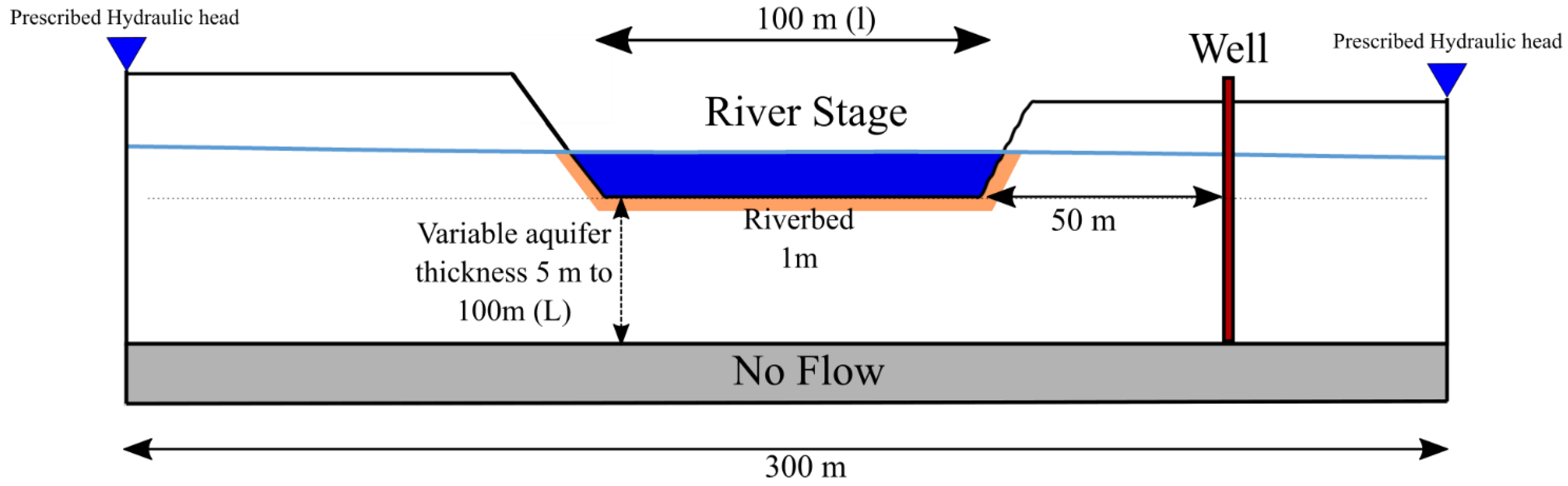
The main goal here was to estimate the natural or anthropogenic conditions leading to the occurrence of a GW flow below a stream (flowpath pattern, GW divide). The case of a fully disconnected stream aquifer was not considered. A primary objective was to characterize the enabling factors for the GW flow: the critical aquifer thickness below a stream (called L on Figure 1) to obtain a horizontal bottom flow not influenced by the river water level, which usually causes the GW flow divide associated with a vertical component of the flow, the streambed properties and the hydraulic head gradient between the two banks.
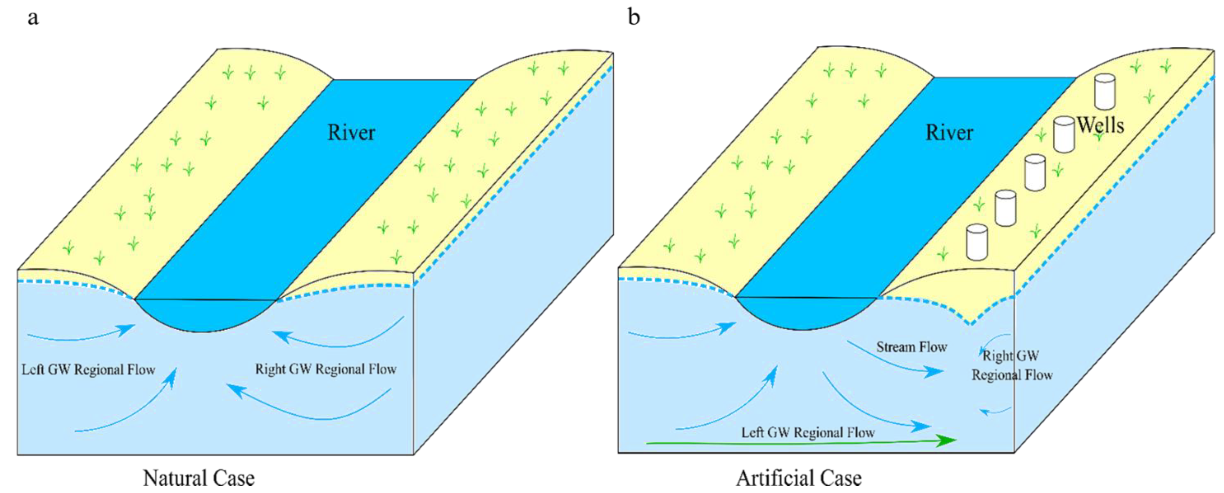
We considered two principal base conditions, a natural situation characterized by a natural hydraulic head gradient from the left bank to the river, and an artificial condition associated with the presence of an alignment of fully penetrating pumping wells on the right bank, which is a common configuration of GW exploitation in alluvial plains [46,51]. The first situation, i.e., the natural condition with a hydraulic head gradient between each bank, is the gaining river reference. The second situation is an artificial condition with the presence of a pumping field on the right bank, located 50 m from the river (Figure 1 and Figure 2). In the latter situation, some other controlling factors were tested, such as variations in the pumping rate or the initial natural gradient, to identify the impact on the water circulation below the river, notably the formation of a horizontal flow between the two banks (left GW regional flow reaching the wells, Figure 2).
We considered two principal base conditions, a natural situation characterized by a natural hydraulic head gradient from the left bank to the river, and an artificial condition associated with the presence of an alignment of fully penetrating pumping wells on the right bank, which is a common configuration of GW exploitation in alluvial plains [40,41,46,51]. The first situation, i.e., the natural condition with a hydraulic head gradient between each bank, is the gaining river reference. The second situation is an artificial condition with the presence of a pumping field on the right bank, located 50 m from the river (Figure 1 and Figure 2). In the latter situation, some other controlling factors were tested, such as variations in the pumping rate or the initial natural gradient, to identify the impact on the water circulation below the river, notably the formation of a horizontal flow between the two banks (Left GW regional flow reaching the wells, Figure 2).
The problem of identifying conditions for the occurrence of bottom horizontal GW flow below a stream, leading to a flow from one bank to the other one (cross-riverbank flow), was addressed by means of numerical modeling (Left GW regional flow, Figure 2). This requires identifying the most appropriate modeling approach. The Dupuit–Forchheimer assumption, which assumes that the flow in the aquifer is predominantly horizontal, is the basis for the water mass balance equation solved for unconfined aquifers in most hydrogeological models. This assumption is, in fact, no longer valid in the vicinity of a stream, notably when the wells are close to the river [52]. Alternatively, the continuity equation within the saturated domain, which is written:
with q Darcy’s specific discharge (m s−1), ρ the water density (kg m−3), ω the porosity, and t the time (s) can be solved. However, the upper limit of the saturated domain, i.e., the water table, is the unknown of the problem, making resolution rather difficult. In order to achieve the objectives of this study, the solution finally adopted consisted of solving variably saturated flow equations in the domain comprising the stream and the aquifer, using the variably saturated finite difference code GINETTE [13,50] that simulates GW flow and the SW–GW exchanges. This model solves Richard’s equation for a 2D (x, z) domain, with x and z being the horizontal and upwards vertical axis. The GW mass balance equation for variably saturated media is written:
where p is the pore water pressure (Pa), Sw is the water saturation, w is a volumetric water source or sink (s−1), is the total porosity, kx and kz are intrinsic permeability along the x and z axes (m2), kr(Sw) is the relative unsaturated hydraulic conductivity, g is the acceleration due to gravity (m s−2), z is the vertical coordinate taken as positive upwards (m) and is the dynamic viscosity of water (Pa s). Two soil hydraulic functions were used to characterize the parameters in the unsaturated zone: the Van Genuchten function [53] for the relationship between the pressure and water saturation (Equation (3)), and the Mualem model [54] for the relative unsaturated hydraulic conductivity (Equation (4)).
where Se is the effective water saturation (—), Sw is the soil water saturation and Srw the residual soil water saturation, pc is the capillary pressure (Pa), α (Pa−1), n and m are Van Genuchten parameters.
Here, we simulate a synthetic case that mimics a high order Strahler stream [55] representative of the great European rivers such as the Rhône River in France [46]. The computational domain represents a cross section of a stream embedded in its aquifer with constant mesh spacing (Figure 1). The total cross section is 300 m wide (x = 0 at the left boundary, positive in the right direction), 100 m deep (z, positive upwards) and 1 m deep, perpendicular to the cross-section. The mesh size is constant (dx = 1 m). The domain consists of 7187 to 64,377 cells depending on the aquifer thickness. The model is constructed with prescribed hydraulic head boundaries on each side, no flow boundary at the bottom, a river level fixed at 16 m (Figure 1), and without recharge. The prescribed hydraulic head conditions make it possible to control the regional head gradient, i.e., the background natural gradient, and these boundaries can correspond to surface water bodies imposing hydraulic head, such as lakes or other rivers. The aspect ratio Ar is the ratio of the aquifer thickness below the streambed L (m) to the width of the river l (m):
The ratio was modified between 0.05 and 1 by varying the thickness of the aquifer (Figure 1).
Furthermore, the impact of a pumping field located on the right bank was introduced in GINETTE using a dedicated water balance equation written as:
where h is the hydraulic head at the borehole (m), SB is the horizontal surface of the borehole (m2), and Qnet|B is the net flux entering the well (m3 s−1).
Here we considered the common situations of an alignment of pumping wells along the river channel (Figure 2b.). Two different pumping rates were tested: 0.01 m3 s−1 m−1 and 0.001 m3 s−1 m−1. These values correspond to the geometry considered here, and thus to pumping rates per meter of a linear field pumping. For a pumping site 100 m in length, these values correspond to a total extraction of 3600 m3 h−1 and 360 m3 h−1.
In addition, three types of streambeds were examined: no clogging layer (the same media as the aquifer), a tenfold less permeable clogging than the porous media of the aquifer, and a clogging one hundred-fold less permeable than the aquifer. The hydrodynamic parameters used here are given in Table 1. In this study, the aquifer was considered homogeneous and isotropic, made of gravel and sand. A homogeneous and isotropic clogging layer made of sandy clay was also considered. A lower hydraulic conductivity than the aquifer for the clogged streambed was assumed, with a minimum value at 10−5 ms−1. The values considered here are consistent with a 100 m wide river characterized by large discharge, and therefore weak clogging associated with small particles, even if lower values can exist in the case of a highly clogged streambed and a small stream with a low river flow [56,57]. The parameters corresponding to sand for the aquifer and sand-clay material for the clogged layers were taken from the literature [58,59].
In a first set of simulations (Sim#1, Table 2), variable pumping rates were considered for the symmetrical situation of a gaining river with a prescribed hydraulic head of 16.5 m on the right and left sides (scenario H0). These variations were tested for the three different clogging situations described above. To study the impact of a regional gradient in the situation of a pumping well field, the hydraulic head of the right boundary was varied (H0: 16.5, H0.5: 16, and H1:15.5 m), with the left boundary fixed at 16.5 m and a river stage at 16 m for an unclogged streambed in a second set of simulations (Sim#2, Table 2). Note that the boundary conditions H0.5 are unlikely in a natural environment, but give a symmetrical water slope around the pumping well (hydraulic head at 16 m in the river and at the right boundary). In situation H1, the hydraulic head prescribed to the right boundary is below the river stage. This condition gives a natural gradient with a flow from the left side to the right side. To identify the role of the different controlling factors (the clogging layer, the regional head gradient, the pumping rate), the contributions of the different compartments (the river and the left and right bank) to the pumping well discharge were calculated. The right GW regional flow supplying the wells is the sum of the flows on all the right sides of the porous media cells neighboring the wells. The left side flow at the wells was divided into two contributions: the streamflow leakage (stream water leaking down to the GW) and the left GW regional flow. The stream leakage was calculated as the output flow from the river’s cells. The left GW regional flow (the water that comes from the left boundary of the domain) was calculated by the difference between the total flow arriving to the left of the wells and the stream leakage.
The impact of the distance between the river and the wells was also analyzed in a third set of simulations (Sim#3, Table 2). Additional simulations were performed considering different distances between the wells and the river (25, 50 and 75 m), using Q = 0.001 m3 s−1 m−1, scenario H0, H0.5 and H1. When the well is moved far away from the riverbank, the well’s feeding area is expected to be restricted to the bank on which the well is located. In this situation, water is no longer supplied by the river and probably not by the left GW regional flow either, at least for gaining rivers (H0 boundary conditions). Although fully penetrating wells were also considered in this study, a fourth set of calculations (Sim#4, Table 2) were made to determine the impact of partially penetrating wells. Two simulations were made with 25 m and 75 m deep wells using assumption H0 and an aquifer depth of 100 m (Ar = 1).
3. Results
3.1. Comparison between Natural and Pumping Situations
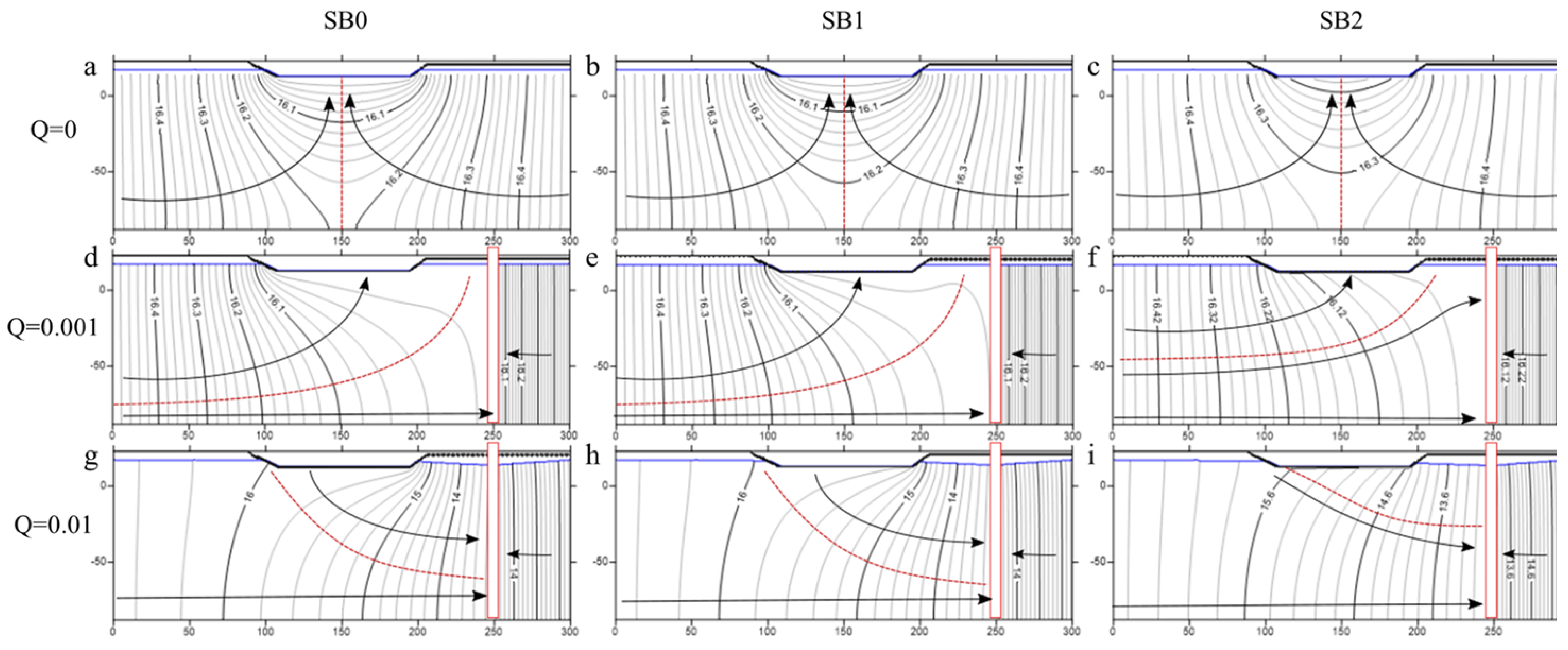
In the natural symmetric situation (Q = 0, Figure 3a–c, Sim$1.1, Sim$1.4 and Sim$1.7, Table 2), GW flow converges to the river in the usual situation of a connected gaining stream. The GW divide is vertical and located at the middle of the stream. Figure 3 illustrates that at Ar = 1, the vertical component of the GW flow below the streambed is significant. For the scenario SB0, the pumping (Q = 0.01 m3 s−1 m−1 or Q = 0.001 m3 s−1 m−1) creates a decrease in the water table level, and the shape of the piezometric lines changes (Figure 3a,d,g). The hydraulic gradient increases with the pumping rate as expected. In these simulations, the hydraulic head gradient is greater on the right side than on the left, so more water from the right side is contributed to the wells. With a pumping rate of 0.001 m3 s−1 m−1, streamlines indicate the characteristics of the flow systems, a divide line exists between the local flow system of the rivers and the regional flow towards the well. This divide line is not vertical and is not located in the center of the river. The flow from the left boundary is divided into two domains (Figure 3d–f). The first domain is located at the top of the aquifer and is characterized by a converging flow towards the river, and the second, at the bottom of the aquifer, converges directly towards the well. In this condition, the SW–GW system remains in upwelling conditions.
With a pumping rate of 0.01 m3 s−1 m−1, the flowpath patterns are no longer separated vertically into two distinct zones, but all the streamlines converge towards the well (Figure 3gh–i). In this condition, the SW–GW connections change to a downwelling configuration, with the flow from the river clearly supplying the well.
The impact of the pumping rate on the proportion of water reaching the wells in the SB0 stream clogging condition (no clogging, Sim$1.2 and Sim$1.3) is summarized in Table 3. The increase in the pumping rate decreases the flow proportion coming from the right side to the wells: it is 96% when Q = 0.001 and 67% for Q = 0.01. Increasing the pumping rate drastically increases the streamflow contribution that reaches the wells from 0% to 26.5%. The left GW regional flow contribution also increases, but more moderately from 4% to 6.5%.
3.2. Impact of the Clogging
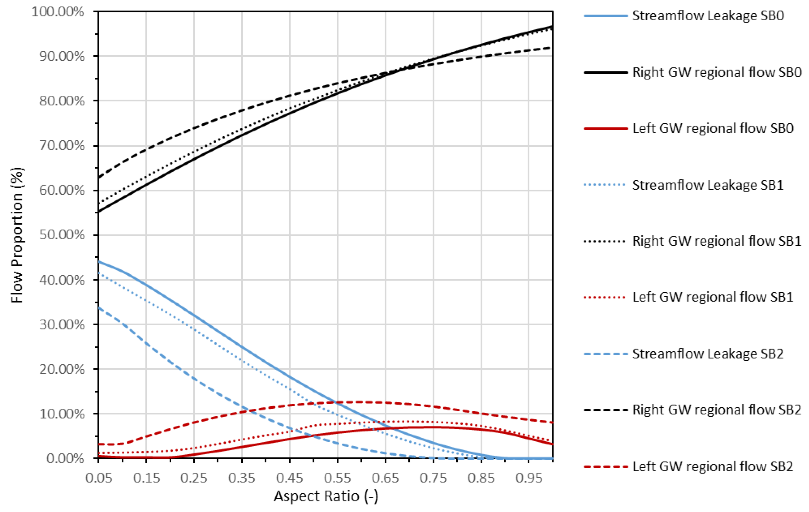
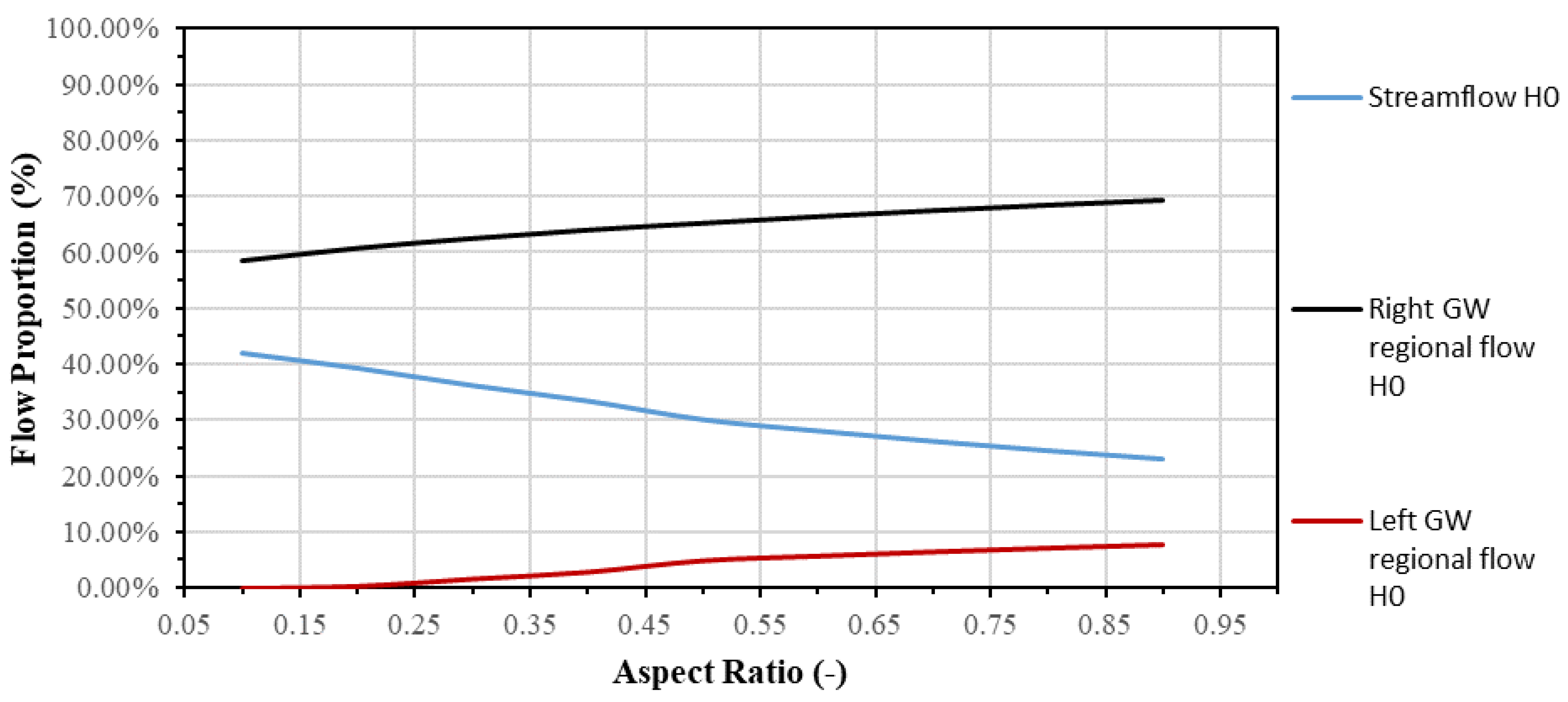
The three scenarios of streambed clogging (SB0, SB1 and SB2) considered here lead to a similar configuration of flowpath patterns, with the vertical component of the water flow (and velocities) at the bottom of the model (Figure 3). Figure 3 also shows the expected decreasing contribution and streamflow contribution as the clogging of the streambed increases (SB0 to SB2 scenarios, Figure 3g–i). Figure 4 shows the flow proportions in the well as a function of the aspect ratio value, for the 0.001 m3 s−1 m−1 pumping rate, and considering the three clogging scenarios (SB0, SB1 and SB2). In the scenario SB0, 45% of the pumping well is supplied by water from the river, and 55% from the right GW regional flow. In SB1 and SB2 clogging situations, the maximum water river contributions to the pumping well are 42% and 34%, respectively. These contributions were simulated for low values of Ar (0.05). For the hydraulic conductivity of the three different streambeds, as the aspect ratio increases, the river water contribution decreases, and the water coming from the right bank increases. The stream–aquifer system is in a complete upwelling condition. Hence, the streamflow contribution becomes negligible with a large value of the aspect ratio (0.85 for SB0 and SB1, 0.7 for SB2). In the SB0 and SB1 streambed clogging conditions, with an aspect ratio larger than 0.2, the left regional GW flow supplies the pumping well. Considering the simulations, including the most clogged streambed (SB2), a horizontal flow occurs even with a low aspect ratio. However, in this situation, less than 5% of the well is supplied by the left regional GW. In all conditions, the water coming from the left regional GW does not exceed 13%.
3.3. Impact of the Natural Hydraulic Head Gradient in the Pumping Condition
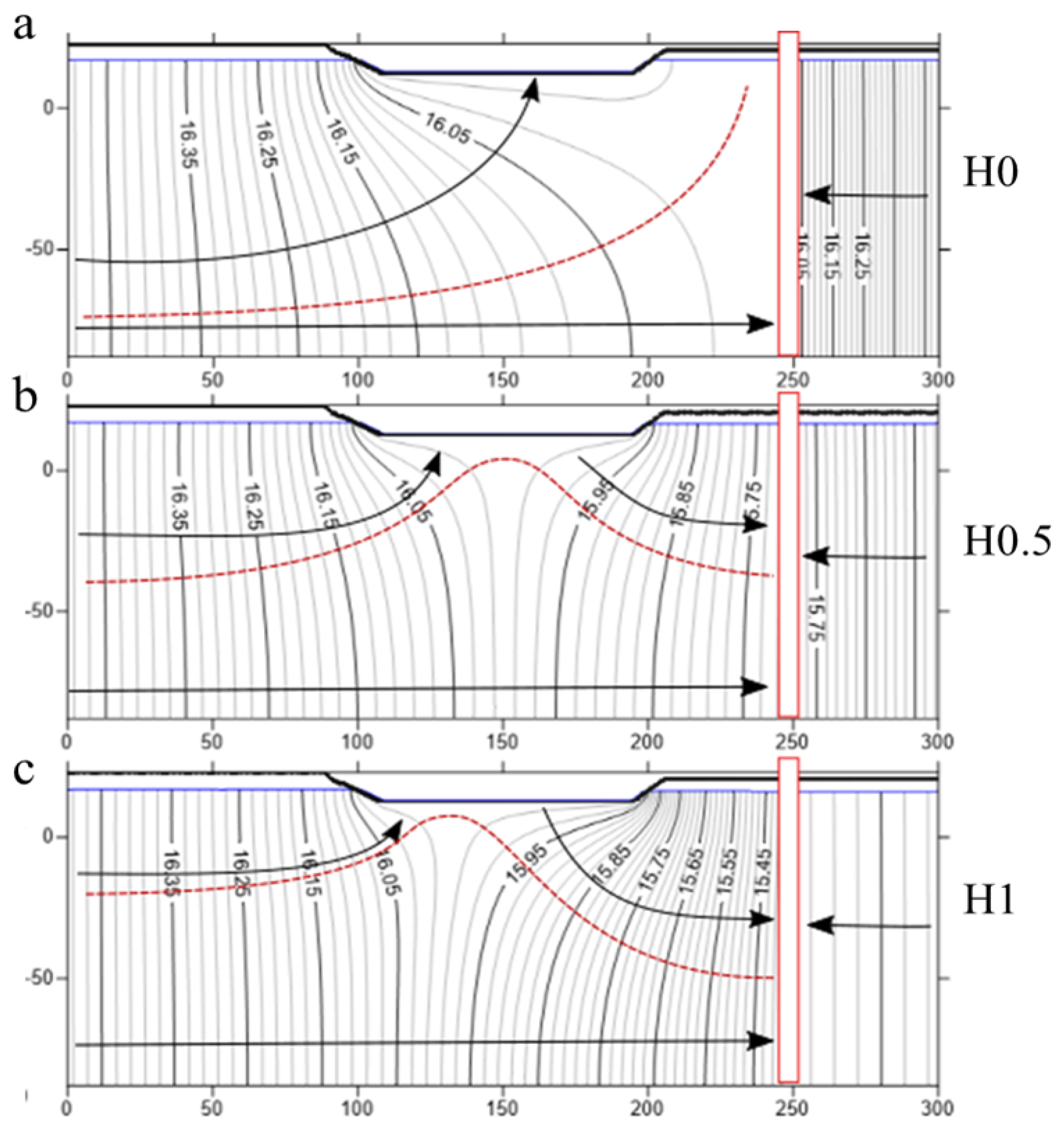
Constant values for the pumping rate and the prescribed hydraulic head at the left boundary of the domain were set at 0.001 m s−1 m−1 and 16.5 m, respectively, while the prescribed head boundary on the right of the domain was varied from 16.5 m to 15.5 m to identify the impact of the hydraulic head gradient for the unclogged layer (Figure 5). The natural hydraulic head gradient condition, i.e., the gaining river (Sim$2.1, Table 2), is the same as the symmetrical situation previously analyzed (Figure 3, SB0, Q = 0.001, Sim$1.3) and is reproduced here just for comparison (Figure 5a). Considering now the scenario H0.5 (Sim$2.2, Table 2), the piezometric level on the right boundary is the same as the river stage (Figure 5b), yielding the same water table slope between the wells and the river as between the wells and the right boundary. Here, this hydraulic head gradient depends only on the pumping rate, since the river stage and the right boundary are the same. The flowpath patterns divide the domain into three zones: two local flow systems of the river (upwelling and downwelling), and the regional flow towards the well. In this condition, the pumping well rate is supplied by both the right and left boundaries and the streamflow leakage. In situation H1, the pattern of the flow pathway is the same as in the previous situation. However, the depth of the upwelling zone is thinner, and the downwelling zone is deeper. The well is mostly supplied by the streamflow leakage and the regional flow, while the contribution of the right boundary weakens (Figure 5). In the three alternative scenarios considered here (Sim$2.1, Sim$2.2 and Sim$2.3, Table 2), the upper part of the aquifer on the left of the domain flows towards the river, and the bottom part shows a horizontal flow below the river which converges to the well. A streamflow leakage is only obtained for the head gradient conditions H0.5 and H1.
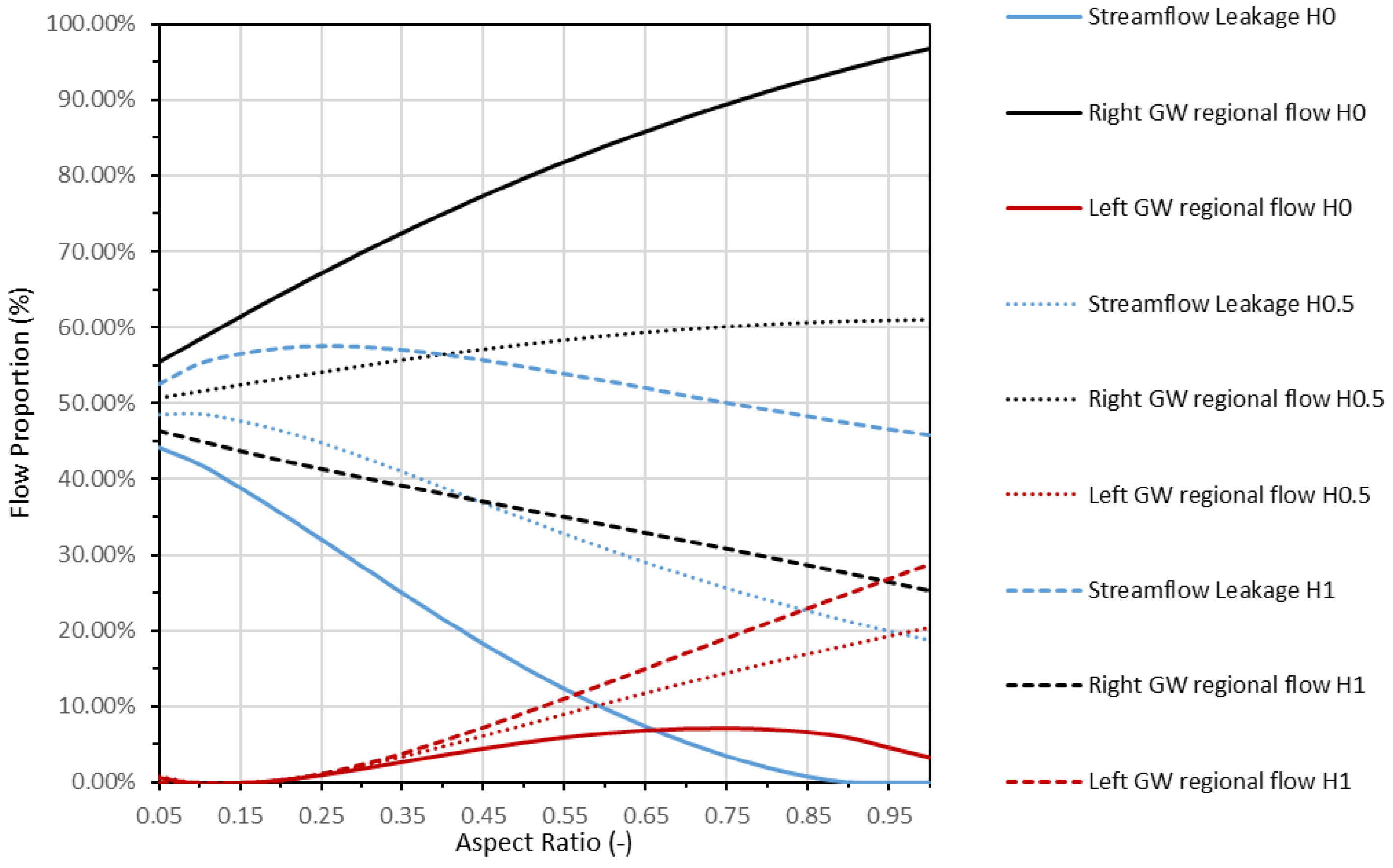
Figure 6 presents the different contributions to the well as a function of the aspect ratio for the different hydraulic head gradient condition (Sim$2.1, Sim$2.2 and Sim$2.3). In all these scenarios, the river contribution to the pumping decreases when the aspect ratio increases. The maximum values are simulated with a low value Ar (0.05): 45% for the H0, 49% for the H0.5, and 53% for the H1 scenarios. For the H0 hydraulic head gradient condition, the river contribution almost vanishes for Ar > 0.9. In the other scenarios (H0.5 and H1), the river still contributes to the well pumping even at Ar = 1 (20% for H0.5 and 45% for H1). Contrary to the river contribution, the right regional GW flow for situations H0 and H0.5 increases with increasing aspect ratio. In the H1 hydraulic head gradient condition, this flow decreases similarly to the streamflow contribution, while the left regional contribution increases. Finally, the horizontal left regional GW flow is largely influenced by the hydraulic scenario (H0, H0.5 and H1). This flow is negligible for aspect ratios below 0.2, but reaches 5% in the H0 condition, 20% for H0.5 and 30% for H1, when Ar is taken at 1.
3.4. Impact of the Distance between the Well and the Riverbank
The influence of the distance of the borehole from the riverbank, which has been considered constant hitherto, is analyzed. The calculated contributions to pumping from the river and the left GW regional flow are 33% and 8%, respectively, for a distance between the wells and the bank of 25 m (Sim$3.3), and 15% and 5% for a distance of 50 m (Sim$3.2). For 75 m (Sim$3.1), the pumping is entirely supplied by the right GW regional flow of the well. Simulations confirm that beyond a critical distance, neither SW nor GW from the left GW regional flow are drained by the well. For wells located closer to the river, the simulations lead to a constant Ar threshold value of 0.2 for cross-riverbank GW flow to occur, regardless of the distance. This is also valid using boundary conditions H0.5 and H1, but with a contribution of the SW and GW from the left GW regional flow irrespective of the distance between the well and the riverbank (Sim$3.4 and Sim$3.7).
3.5. Effect of Non-Penetrating Well
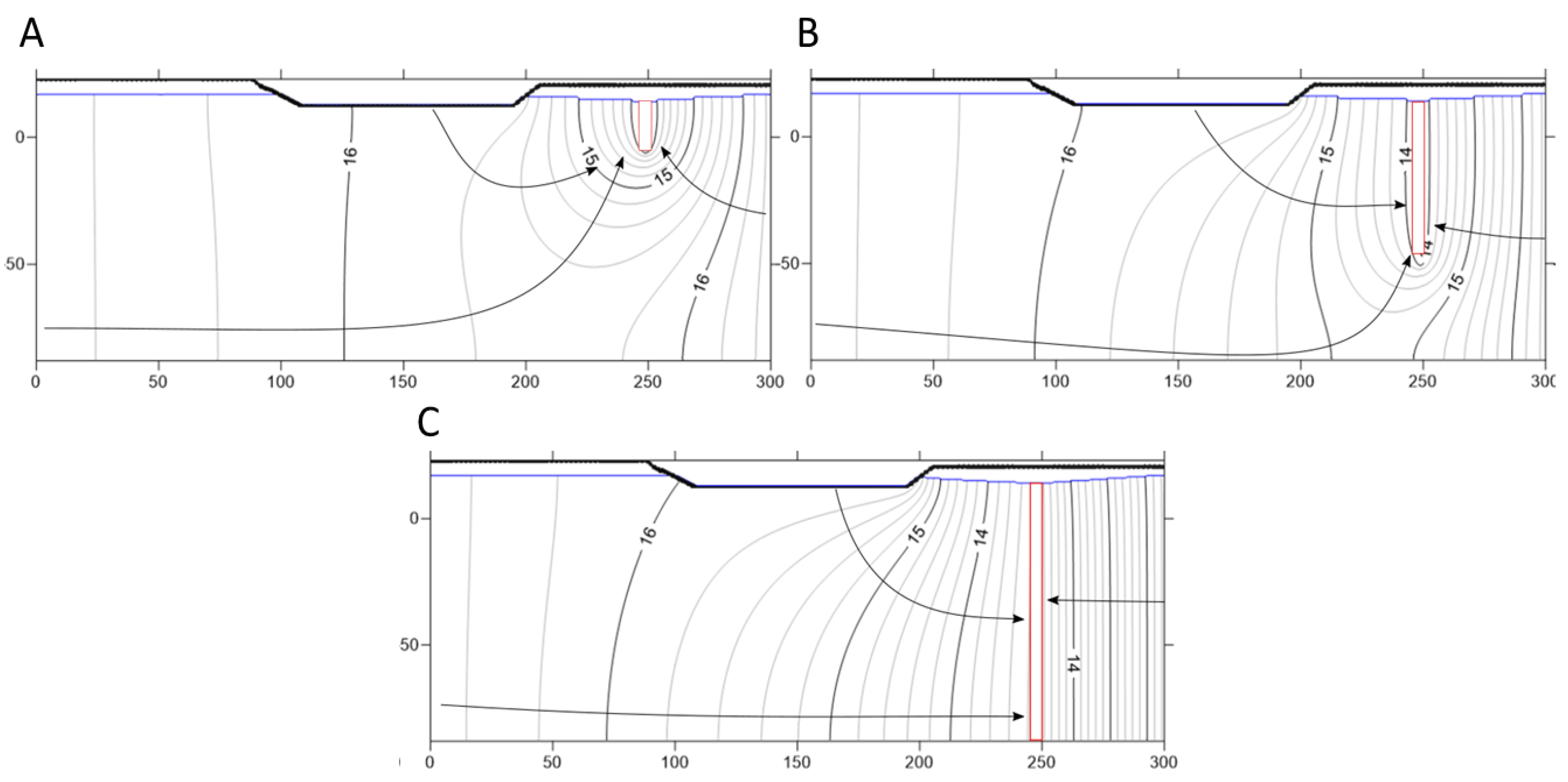
Figure 7 shows the change in flowpath patterns when the wells are not fully penetrating, with 25 and 75 m deep wells for the H0 hydraulic gradient condition (Sim$4.1 and Sim$4.2) and an aquifer depth of 100 m (Ar = 1). The well depth impacts the pumping area around the wells, changes flow directions, and enhances the contribution to the pumping from the right side in the case of shallow wells (Figure 7). The river contribution is almost independent of the well depth and remains around 25% (Table 4). Only the relative proportions supplied by the two riverbanks are impacted. More water is drained from the right GW regional flow and, conversely, the contribution from the left GW regional flow is reduced when the wells are shallower (Table 4).
4. Discussion
The simulations presented in this study confirm the possibility of no vertical GW divide, and a GW flow from one riverbank to the opposite one (cross-river bank flow), independently of the streambed properties in anthropized (pumping) situations. The controlling factors identified during the numerical simulations conducted here, i.e., the aspect ratio (Ar, Equation 5), the hydraulic conductivity of the streambed, the natural local hydraulic head gradient, the well-river distance, and the fully or partially penetrating state of the well have to now be further analyzed and discussed.
The hydraulic head gradients between the river and the well, and between the right boundary and the well, which depend on the selected scenario (H0, H0.5, or H1), are a key feature to understand the contributions to the pumping illustrated in Figure 5. This is due to the sharing of the left flow between the local flow system of the river and the regional flow. The hydraulic head gradient influences the SW–GW connectivity (upwelling and downwelling). In the H0 condition, the right boundary at 16.5 m causes a large hydraulic head gradient on the right of the well. Therefore, a prominent fraction of GW converging to the well from this side is simulated. The horizontal left regional GW flow, and the river contribution are low even at large aspect ratios. In the H1 condition, the opposite situation is simulated with a large hydraulic head gradient between the river and the well, a low contribution from the right side of the well, and an enhanced horizontal flow coming from the left riverbank below the streambed. In the simulation H0.5, with the same hydraulic head gradient on the left and right side of the well, for small aspect ratios, the proportion of flows coming from the river and from the right side of the pumping field are similar. In these hydraulic conditions, the low thickness of the aquifer promotes stream leakage. As the aquifer thickness increases, the flow coming from the right part of the domain increases while the contribution of the river water decreases. The left horizontal GW flow increases with the aquifer thickness.
Considering partially penetrating wells, increasing the well depth leads to a larger contribution from the left GW regional flow and related flow below the river. From a water management standpoint, using fully penetrating wells maximizes the efficiency of GW exploitation, but enhances the contribution from the riverbank opposite to the wells with potential quality issues.
This study shows that for a very thin aquifer below the river, i.e., Ar less than 0.2, the flow coming from the left side is negligible (Table 5). This value of Ar can be considered a threshold value. In this case, the wells are mainly supplied by local flows from the river and from the right regional GW flow. This is almost consistent with the result obtained by Bower (1969) for unclogged rivers who showed that a partially penetrating river behaves as a fully penetrating river, preventing any cross-riverbank flow for Ar < 0.33 (Table 5). In this study, we show that this ratio of Ar < 0.33 proposed by Bower (1969) is lower and that Ar < 0.2 prevents cross-riverbank flow for an unclogged river. Streambed clogging by isolating the river system reduces the proportion of streamflow in the wells, therefore increasing, especially for small aspect ratios, the right GW regional flow. Conversely, with high aspect ratios, the left GW regional flow is favored (Figure 4). For a streambed with a hydraulic conductivity two orders of magnitude lower than the aquifer, the left GW regional flow represents 8% of the well water for Ar = 0.25 and 4% for Ar = 0.05 (Table 5).
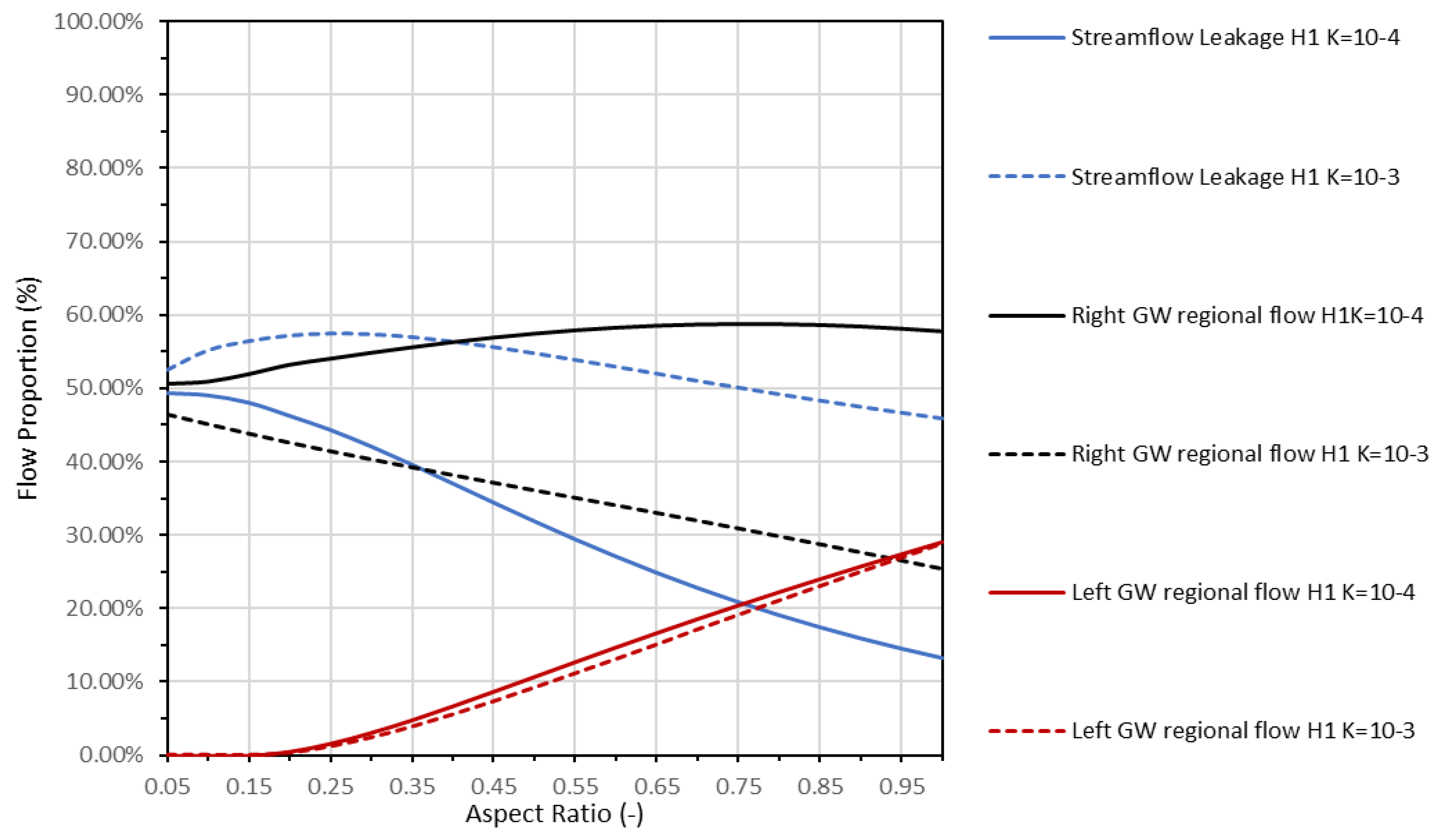
For the H0 scenario, the simulated contribution of the left GW regional flow feeding the pumping increases until Ar = 0.8 and then decreases (Figure 4 and Figure 6). This behavior, which is not observed for the other two scenarios, can be readily explained by a combination of calculated hydraulic head gradients and a constant pumping rate. Increasing the aspect ratio yields larger transmissivity which in turn leads to a larger relative contribution from the domain on the right of the wells, especially in the H0 condition (Figure 5a) of a gaining river with a natural head gradient oriented towards the river and, thus, the wells. At a constant pumping rate, as considered here, increasing the aspect ratio decreases the lateral velocity around the well, producing a similar effect to a pumping rate reduction. This may affect the relative contributions of the different compartments of the system to the wells and explain the decrease in the cross-riverbank flow at Ar > 0.8 for the H0 condition (Figure 6, H0, Sim$2.1, Sim$2.2 and Sim$2.3). This bias was verified by means of additional simulations shown in Appendix A. The calculations demonstrate that, assuming a linear increase in the pumping rate with the aspect ratio, the previous results obtained for H0.5 (Sim$2.2) and H1 (Sim$2.3) are unchanged, but the left GW regional flow fraction decrease previously calculated for H0 (Sim$2.1) at Ar > 0.8 is no longer obtained. A sensitivity analysis to the saturated hydraulic conductivity was conducted by considering a value at 10−4 m s−1 without changing the threshold value for Ar, which remains at 0.2, as well as the contribution of the cross-riverbank flow (see Appendix B). However, as the permeability decreases, the contribution to the pumping coming from the river decreases, while that from the right GW regional flow increases.
Regarding the well–river distance effect, moving the borehole away from the river simply cancels the surface water supply to the well in the H0 head gradient condition as the catchment area of the well is then restricted to the right side of the domain. Since our study focuses on the conditions required to drain the opposite riverbank groundwater, the situation of a catchment area of the pumping well disconnected from the river is not considered. Therefore, the proposed threshold Ar > 0.2 is valid in situations of a river drained by a pumping well. This is the case unconditionally in situations H1, H0.5 and H0, when the wells are less than 50 m from the river. In the condition H1, when pumping is on a bank supplied by the river, simulations show that when the well is moved farther away, the contribution from the surface water and the left GW regional flow decrease, but the threshold at 0.2 for Ar remains valid, as for H0. However, contrary to H0, when the well is 75 m from the river, pumping continues to drain the river water and left boundary water. Overall, cross-riverbank flow can occur when Ar > 0.2 and surface water is drained from the river to the pumping.
Sensitivity analysis has highlighted conditions allowing cross-river corridor horizontal GW. In cases where this flow is possible and a source of contamination was identified on the left bank, this points to a risk of pollution of the wells on the opposite bank. Since the flow below the river is maximum at the bottom of the aquifer, the densest pollutants are likely to flow at higher concentrations to the well [60]. This problem could be enhanced in the condition of fully penetrating wells that are only screened in the lower part of the aquifer. The problem is maximized if this kind of well is closer to the river and the streambed is clogged.
In the old, simplified vision, the river is considered as a drain, the GW flow converges towards the river, and the horizontal flow below the river is not considered. Conversely, situations with a local hydraulic head gradient, i.e., with a lower hydraulic head on the right boundary (H1), enhance this horizontal flow. Such hydraulic conditions can be encountered in situations of a pumping field between two rivers with different stages. In these conditions, the flow from the left side and the river will be favored, and the flow below the river will increase as the aspect ratio also increases.
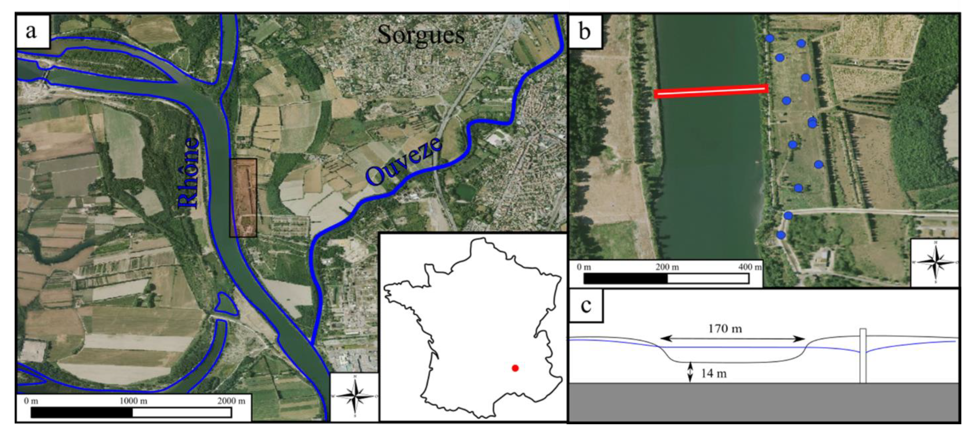
It is therefore important to consider the possible occurrence of this type of flow when working at the local scale. Neglecting the possibility of these horizontal flows may lead to an underestimation of the vulnerability of pumping. Considering or discarding this effect requires estimating the clogging of the streambed and the aspect ratio (thickness of the aquifer below the river), which may play an important role in the exchanges between aquifer and rivers. An illustrative case is provided by a well field located near the city of Sorgue (France, Figure 8) [46,48] on the left bank of the Rhône River. The configuration of the riverbank pumping well, which corresponds to our numerical simulations, is depicted in Figure 8b. The stream-aquifer system with about a 14-m thickness for the aquifer below the streambed, and with a river width of 170 m is characterized by an Ar value of about 0.08. This Ar value suggests a negligible contribution from the left riverbank, enabling a simple interpretation of ongoing tracer experiments. Another example of an unfavorable situation for cross-riverbank flow is provided by Zhu et al. [40] for the Song Hua River (China), characterized by a width of 400 m and a local aquifer thickness of 35 m (Ar < 0.1). Well field supply sources restricted to the riverbank containing the wells were confirmed by means of a geochemical analysis (major ions) leading to a river water fraction of between 40 and 60% depending on the well and the remaining fraction made of local groundwater.
In contrast to the first two examples, cross-riverbank flows were identified in Germany, for the Elbe river at a location where it is 100 m wide and the aquifer is 18 m thick leading to the Ar of 0.18 [61]. Albeit slightly below our threshold at 0.2, a significant clogging streambed explains the occurrence of this underflow, which is consistent with our simulations (Sim$1.8 and Sim$1.9). This cross-riverbank flow was evidenced by the contamination of the well field by nitrates originating from the opposite bank. By means of numerical simulations, the authors estimated a contribution of groundwater from the opposite bank to the pumping of between 5% and 15%. A final illustration of cross-riverbank flow occurrence is provided by Przybyłek et al. [62] for a well field aligned along the Warta River (Poland). The Ar ratio at 0.55, corresponding to a river width of 55m and an aquifer thickness of 30m, is consistent with this observation based on water level surveys.
Beyond these few examples, aquifer water abstractions in near-surface water bodies are a common case, and determining the fractions of the different pumping supplying sources is often difficult in the field. The use of a criterion such as the aspect ratio can help to target investigations and to constrain the mixing to interpret the tracer study. In addition, this threshold allows the identification of the role of the river as a boundary condition or not in the regional model, and thus to limit the model domain.
5. Conclusions
In this study, we investigated the problem of GW flow below a stream in the case of a connected river-aquifer system. The objective was to determine the main parameters controlling the formation of a horizontal GW flow from the left boundary of a valley to a well field located on the right bank. This exchange system between river and aquifer was simulated using the variably saturated model GINETTE with different pumping rates numerically introduced here and for different hydraulic situations: (i) the natural and common case of a gaining river and artificial cases of a gaining river, (ii) a regional hydraulic gradient, produced by the difference between the left and right boundaries of the system. Using these different modeling scenarios, we identified the conditions for GW flow to occur below the streambed from one bank to the other at the local scale. The results and sensitivity analysis showed that the cross-riverbank GW flow below the river is negligible at a low aspect ratio (Ar < 0.2), without streambed clogging. However, this cross-riverbank GW flow can represent between 20 and 30% of the well discharge when the aquifer thickness below the river is high (Ar > 0.8). This flow increases as the aspect ratio increases and is also enhanced by river clogging. We also highlighted the role of the local gradient, which modulates the water table slope around the well, and thus the supply of the well by the river and the horizontal flow below the river.
This type of flow can occur even without streambed clogging. Indeed, a large aspect ratio is sufficient to allow a significant proportion of the water to flow below the streambed. In the context of hydrological numerical modeling, our threshold Ar allows the identification of the role of the river as a boundary condition or not, and thus to limit the model domain. In the case where cross-riverbank flow is likely to occur, the model must take into account the other bank of the river and therefore shift context of groundwater flow numerical modeling. In addition, our criterion Ar can be a tool to support geochemical mixing calculations without the help of numerical simulations. Ar can determine the number of mixing poles (the river, the groundwater at the pumped bank and/or the groundwater from the opposite bank).
The results obtained here may have an impact for local studies on pumping fields located between surface water bodies imposing hydraulic head, such as lakes or rivers at different stages, therefore causing local hydraulic head gradients and favoring the horizontal flow below a stream. The impact of drawdowns of GW level could influence the mixing and dispersion processes in the aquifer below the river. Therefore, this cross-riverbank GW circulation may increase the wells’ vulnerability to pollutants coming from the opposite bank. This direct convective transport below the river may be superimposed to the kinematic dispersion process, which is enhanced in case of migration of the groundwater divide towards the well, as calculated here. Further investigations, considering the transport of pollutants and these different mechanisms, would be desirable.
Author Contributions
Conceptualization, J.T., J.G. and A.R.; Investigation, J.T.; Methodology, J.T., J.G. and A.R.; Software, J.T., J.G. and A.R.; Supervision, J.G.; Visualization, J.T.; Writing—original draft, J.T.; Writing—review & editing, J.T., J.G. and A.R. All authors have read and agreed to the published version of the manuscript.
Funding
This research was funded by the Rhône Mediterranean Corsica Water Agency and the Syndicat Rhône Ventoux.
Institutional Review Board Statement
Not applicable.
Informed Consent Statement
Not applicable.
Data Availability Statement
All analyzed data in this study have been included in the manuscript. This article is based on simulation runs using the Ginette code [13,50], which was developed to study GW–SW interactions for a 2D variably saturated flow using a finite-difference numerical scheme. More information on the computing method is given in the Methodological Approach section, and the validation of the model was made in the Rivière et al. (2014) article. The simulation configurations and parameterizations are also given in the Methodological Approach section. All the calculation and treatment equations, notably the calculation of the water proportions, are also given in the Methodological Approach section. The code used is available here: https://github.com/agnes-riviere/ginette/ (https://doi.org/10.5281/zenodo.4058821) (accessed on 21 January 2022). Additional data as simulation runs are available here (https://nuage.osupytheas.fr/s/wY5GSRX7nczjFYK) (accessed on 21 January 2022).
Acknowledgments
This research has been supported by funding from the Rhône MediterraneanCorsica Water Agency and the Syndicat Rhône Ventoux. The four anonymous referees are acknowledged for their relevant and constructive comments that enabled a substantial improvement of the manuscript.
Conflicts of Interest
The authors declare no conflict of interest.
Appendix A
Figure A1.
Fractions of water feeding the pumping WELL as a function of the aspect ratio for a variable pumping flow (Q = 0.01 *Ar).
Figure A1.
Fractions of water feeding the pumping WELL as a function of the aspect ratio for a variable pumping flow (Q = 0.01 *Ar).

Appendix B
Figure A2.
Evolution of the proportion of water in the pumping well with the aspect ratio for the hydraulic head gradient condition H1 and for a hydraulic conductivity of 10−3 m s−1 (Sim$2.3) and 10−4 m s−1.
Figure A2.
Evolution of the proportion of water in the pumping well with the aspect ratio for the hydraulic head gradient condition H1 and for a hydraulic conductivity of 10−3 m s−1 (Sim$2.3) and 10−4 m s−1.

References
- Maréchal, J.-C.; Rouillard, J. Groundwater in France: Resources, use and management issues. In Sustainable Groundwater Management; Springer: Berlin/Heidelberg, Germany, 2020; pp. 17–45. [Google Scholar]
- Winter, T.C.; Harvey, J.W.; Franke, O.L.; Alley, W.M. Ground Water and Surface Water-A Single Resource-U.S. Geological Survey Circular 1139; U.S. Geological Survey, Water Resources Division: Reston, VA, USA, 1998; Volume Circular, ISBN 0607893397. [Google Scholar]
- Holman, I.P. Climate change impacts on groundwater recharge-uncertainty, shortcomings, and the way forward? Hydrogeol. J. 2006, 14, 637–647. [Google Scholar] [CrossRef] [Green Version]
- Fleckenstein, J.H.; Krause, S.; Hannah, D.M.; Boano, F. Groundwater-surface water interactions: New methods and models to improve understanding of processes and dynamics. Adv. Water Resour. 2010, 33, 1291–1295. [Google Scholar] [CrossRef]
- Krause, S.; Freer, J.; Hannah, D.M.; Howden, N.J.K.; Wagener, T.; Worrall, F. Catchment similarity concepts for understanding dynamic biogeochemical behaviour of river basins. Hydrol. Process. 2014, 28, 1554–1560. [Google Scholar] [CrossRef] [Green Version]
- Bernard-Jannin, L.; Sun, X.; Teissier, S.; Sauvage, S.; Sánchez-Pérez, J.M. Spatio-temporal analysis of factors controlling nitrate dynamics and potential denitrification hot spots and hot moments in groundwater of an alluvial floodplain. Ecol. Eng. 2017, 103, 372–384. [Google Scholar] [CrossRef] [Green Version]
- Malama, B.; Pritchard-Peterson, D.; Jasbinsek, J.J.; Surfleet, C. Assessing stream-aquifer connectivity in a coastal California watershed. Water 2021, 13, 416. [Google Scholar] [CrossRef]
- Ranalli, A.J.; Macalady, D.L. The importance of the riparian zone and in-stream processes in nitrate attenuation in undisturbed and agricultural watersheds-A review of the scientific literature. J. Hydrol. 2010, 389, 406–415. [Google Scholar] [CrossRef]
- Shuai, P.; Cardenas, M.B.; Knappett, P.S.K.; Bennett, P.C.; Neilson, B.T. Denitrification in the banks of fluctuating rivers: The effects of river stage amplitude, sediment hydraulic conductivity and dispersivity, and ambient groundwater flow. Water Resour. Res. 2017, 53, 7951–7967. [Google Scholar] [CrossRef]
- Brunner, P.; Simmons, C.T.; Cook, P.G. Spatial and temporal aspects of the transition from connection to disconnection between rivers, lakes and groundwater. J. Hydrol. 2009, 376, 159–169. [Google Scholar] [CrossRef] [Green Version]
- Brunner, P.; Cook, P.G.; Simmons, C.T. Hydrogeologic controls on disconnection between surface water and groundwater. Water Resour. Res. 2009, 45, 1–13. [Google Scholar] [CrossRef] [Green Version]
- Fuchs, E.H.; King, J.P.; Carroll, K.C. Quantifying Disconnection of Groundwater from Managed-Ephemeral Surface Water during Drought and Conjunctive Agricultural Use. Water Resour. Res. 2019, 55, 5871–5890. [Google Scholar] [CrossRef] [Green Version]
- Rivière, A.; Gonçalvès, J.; Jost, A.; Font, M. Experimental and numerical assessment of transient stream-aquifer exchange during disconnection. J. Hydrol. 2014, 517, 574–583. [Google Scholar] [CrossRef] [Green Version]
- Simonds, F.W.; Sinclair, K.A. Surface Water-Ground Water Interactions Along the Lower Dungeness River and Vertical Hydraulic Conductivity of Surface Water-Ground Water Interactions Along the Lower Dungeness River and Vertical Hydraulic Conductivity of Streambed Sediments, Clallam Cou. USGS Prof. Pap. 2002, 2, 20327. [Google Scholar]
- Cardenas, M.B. A model for lateral hyporheic flow based on valley slope and channel sinuosity. Water Resour. Res. 2009, 45, 1–5. [Google Scholar] [CrossRef] [Green Version]
- Cardenas, M.B.; Wilson, J.L.; Zlotnik, V.A. Impact of heterogeneity, bed forms, and stream curvature on subchannel hyporheic exchange. Water Resour. Res. 2004, 40, 1–14. [Google Scholar] [CrossRef] [Green Version]
- Pryshlak, T.T.; Sawyer, A.H.; Stonedahl, S.H.; Soltanian, M.R. Multiscale hyporheic exchange through strongly heterogeneous sediments. Water Resour. Res. 2015, 51, 9127–9140. [Google Scholar] [CrossRef] [Green Version]
- Sawyer, A.H.; Cardenas, M.B. Hyporheic flow and residence time distributions in heterogeneous cross-bedded sediment W08406. Water Resour. Res. 2009, 45, 1–12. [Google Scholar] [CrossRef] [Green Version]
- Pinay, G.; Peiffer, S.; De Dreuzy, J.R.; Krause, S.; Hannah, D.M.; Fleckenstein, J.H.; Sebilo, M.; Bishop, K.; Hubert-Moy, L. Upscaling Nitrogen Removal Capacity from Local Hotspots to Low Stream Orders’ Drainage Basins. Ecosystems 2015, 18, 1101–1120. [Google Scholar] [CrossRef] [Green Version]
- Clausen, L.; Fabricius, I.; Madsen, L. Adsorption of Pesticides onto Quartz, Calcite, Kaolinite, and α-Alumina. J. Environ. Qual. 2001, 30, 846–857. [Google Scholar] [CrossRef] [PubMed]
- Song, X.; Chen, X.; Stegen, J.; Hammond, G.; Song, H.S.; Dai, H.; Graham, E.; Zachara, J.M. Drought Conditions Maximize the Impact of High-Frequency Flow Variations on Thermal Regimes and Biogeochemical Function in the Hyporheic Zone. Water Resour. Res. 2018, 54, 7361–7382. [Google Scholar] [CrossRef]
- Cardenas, M.B. Stream-aquifer interactions and hyporheic exchange in gaining and losing sinuous streams. Water Resour. Res. 2009, 45, 1–13. [Google Scholar] [CrossRef]
- Flipo, N.; Mouhri, A.; Labarthe, B.; Biancamaria, S.; Rivière, A.; Weill, P. Continental hydrosystem modelling: The concept of nested stream & ndash;aquifer interfaces. Hydrol. Earth Syst. Sci. 2014, 18, 3121–3149. [Google Scholar] [CrossRef] [Green Version]
- Barthel, R.; Banzhaf, S. Groundwater and Surface Water Interaction at the Regional-scale–A Review with Focus on Regional Integrated Models. Water Resour. Manag. 2016, 30, 1–32. [Google Scholar] [CrossRef] [Green Version]
- Toth, J. A Theoretical Analysis of Groundwater Flow in Small Drainage Basins 1 of phe low order stream and having similar t he outlet of lowest impounded body of a relatively. J. Geophys. Res. 1963, 68, 4795–4812. [Google Scholar] [CrossRef]
- Goderniaux, P.; Davy, P.; Bresciani, E.; De Dreuzy, J.R.; Le Borgne, T. Partitioning a regional groundwater flow system into shallow local and deep regional flow compartments. Water Resour. Res. 2013, 49, 2274–2286. [Google Scholar] [CrossRef] [Green Version]
- Bresciani, E.; Goderniaux, P.; Batelaan, O. Hydrogeological controls of water table-land surface interactions. Geophys. Res. Lett. 2016, 43, 9653–9661. [Google Scholar] [CrossRef]
- Khan, H.H.; Khan, A. Groundwater and Surface Water Interaction. In GIS and Geostatistical Techniques for Groundwater Science; Elsevier Inc.: Amsterdam, The Netherlands, 2019; ISBN 9780128154137. [Google Scholar]
- Gleeson, T.; Wada, Y.; Bierkens, M.F.P.; Van Beek, L.P.H. Water balance of global aquifers revealed by groundwater footprint. Nature 2012, 488, 197–200. [Google Scholar] [CrossRef] [PubMed]
- Saleh, F.; Flipo, N.; Habets, F.; Ducharne, A.; Oudin, L.; Viennot, P.; Ledoux, E. Modeling the impact of in-stream water level fluctuations on stream-aquifer interactions at the regional scale. J. Hydrol. 2011, 400, 490–500. [Google Scholar] [CrossRef]
- Pryet, A.; Labarthe, B.; Saleh, F.; Akopian, M.; Flipo, N. Reporting of Stream-Aquifer Flow Distribution at the Regional Scale with a Distributed Process-Based Model. Water Resour. Manag. 2015, 29, 139–159. [Google Scholar] [CrossRef]
- Hunt, B. Review of Stream Depletion Solutions, Behavior, and Calculations. J. Hydrol. Eng. 2014, 19, 167–178. [Google Scholar] [CrossRef]
- Huang, C.S.; Yang, T.; Yeh, H. Der Review of analytical models to stream depletion induced by pumping: Guide to model selection. J. Hydrol. 2018, 561, 277–285. [Google Scholar] [CrossRef]
- Zipper, S.C.; Gleeson, T.; Kerr, B.; Howard, J.K.; Rohde, M.M.; Carah, J.; Zimmerman, J. Rapid and Accurate Estimates of Streamflow Depletion Caused by Groundwater Pumping Using Analytical Depletion Functions. Water Resour. Res. 2019, 55, 5807–5829. [Google Scholar] [CrossRef]
- Alley, W.M.; Healy, R.W.; LaBaugh, J.W.; Reilly, T.E. Flow and storage in groundwater systems. Science 2002, 296, 1985–1990. [Google Scholar] [CrossRef] [PubMed] [Green Version]
- Barlow, P.; Leake, S. Streamflow Depletion by Wells—Understanding and Managing the Effects of Groundwater Pumping on Streamflow; U.S. Geological Survey, Water Resources Division: Reston, VA, USA, 2012; ISBN 9781411334434. [Google Scholar]
- Konikow, L.F.; Leake, S.A. Depletion and capture: Revisiting “the source of water derived from wells”. Ground Water 2014, 52, 100–111. [Google Scholar] [CrossRef] [PubMed]
- Leake, S.A.; Reeves, H.W.; Dickinson, J.E. A new capture fraction method to map how pumpage affects surface water flow. Ground Water 2010, 48, 690–700. [Google Scholar] [CrossRef] [PubMed]
- Hiscock, K.M.; Grischek, T. Attenuation of groundwater pollution by bank filtration. J. Hydrol. 2002, 266, 139–144. [Google Scholar] [CrossRef] [Green Version]
- Zhu, Y.; Zhai, Y.; Teng, Y.; Wang, G.; Du, Q.; Wang, J.; Yang, G. Water supply safety of riverbank filtration wells under the impact of surface water-groundwater interaction: Evidence from long-term field pumping tests. Sci. Total Environ. 2020, 711, 135141. [Google Scholar] [CrossRef] [PubMed]
- Zhu, Y.; Zhai, Y.; Du, Q.; Teng, Y.; Wang, J.; Yang, G. The impact of well drawdowns on the mixing process of river water and groundwater and water quality in a riverside well field, Northeast China. Hydrol. Process. 2019, 33, 945–961. [Google Scholar] [CrossRef]
- Masse-Dufresne, J.; Baudron, P.; Barbecot, F.; Patenaude, M.; Pontoreau, C.; Proteau-Bédard, F.; Menou, M.; Pasquier, P.; Veuille, S.; Barbeau, B. Anthropic and Meteorological Controls on the Origin and Quality of Water at a Bank Filtration Site in Canada. Water 2019, 11, 2510. [Google Scholar] [CrossRef] [Green Version]
- Woessner, W.W. Stream and fluvial plain ground water interactions: Rescaling hydrogeologic thought. Ground Water 2000, 38, 423–429. [Google Scholar] [CrossRef]
- Bear, J. Hydraulics of Groundwater; McGraw-Hill: New York, NY, USA, 1979. [Google Scholar]
- Miracapillo, C.; Morel-Seytoux, H.J. Analytical solutions for stream-aquifer flow exchange under varying head asymmetry and river penetration: Comparison to numerical solutions and use in regional groundwater models. Water Resour. Res. 2014, 50, 1410–1432. [Google Scholar] [CrossRef]
- Poulain, A.; Marc, V.; Gillon, M.; Cognard-Plancq, A.L.; Simler, R.; Babic, M.; Leblanc, M. Multi frequency isotopes survey to improve transit time estimation in a situation of river-aquifer interaction. Water 2021, 13, 2695. [Google Scholar] [CrossRef]
- Tzoraki, O.; Nikolaidis, N.P.; Cooper, D.; Kassotaki, E. Nutrient mitigation in a temporary river basin. Environ. Monit. Assess. 2014, 186, 2243–2257. [Google Scholar] [CrossRef]
- Poulain, A.; Marc, V.; Gillon, M.; Mayer, A.; Cognard-Plancq, A.L.; Simler, R.; Babic, M.; Leblanc, M. Enhanced pumping test using physicochemical tracers to determine surface-water/groundwater interactions in an alluvial island aquifer, river Rhône, France. Hydrogeol. J. 2021, 29, 1569–1585. [Google Scholar] [CrossRef]
- Grenier, C.; Anbergen, H.; Bense, V.; Chanzy, Q.; Coon, E.; Collier, N.; Costard, F.; Ferry, M.; Frampton, A.; Frederick, J.; et al. Groundwater flow and heat transport for systems undergoing freeze-thaw: Intercomparison of numerical simulators for 2D test cases. Adv. Water Resour. 2018, 114, 196–218. [Google Scholar] [CrossRef]
- Rivière, A.; Jost, A.; Gonçalvès, J.; Font, M. Pore water pressure evolution below a freezing front under saturated conditions: Large-scale laboratory experiment and numerical investigation. Cold Reg. Sci. Technol. 2019, 158, 76–94. [Google Scholar] [CrossRef]
- Loizeau, S.; Rossier, Y.; Gaudet, J.P.; Refloch, A.; Besnard, K.; Angulo-Jaramillo, R.; Lassabatere, L. Water infiltration in an aquifer recharge basin affected by temperature and air entrapment. J. Hydrol. Hydromech. 2017, 65, 222–233. [Google Scholar] [CrossRef] [Green Version]
- Bouwer, H. Theory of seepage from open channels. Adv. Hydrosci. 1969, 5, 121–172. [Google Scholar]
- Van Genuchten, M.T. A Closed-form Equation for Predicting the Hydraulic Conductivity of Unsaturated Soils. Soil Sci. Soc. Am. J. 1980, 44, 892–898. [Google Scholar] [CrossRef] [Green Version]
- Mualem, Y. A new model for predicting the hydraulic conductivity of unsaturated porous media. Water Resour. Res. 1976, 12, 513–522. [Google Scholar] [CrossRef] [Green Version]
- Strahler, A.N. Quantitative analysis of watershed geomorphology. Eos. Trans. Am. Geophys. Union 1957, 38, 913–920. [Google Scholar] [CrossRef] [Green Version]
- Calver, A. Riverbed Permeabilities: Information from Pooled Data. Ground Water 2001, 39, 546–553. [Google Scholar] [CrossRef] [PubMed]
- Datry, T.; Lamouroux, N.; Thivin, G.; Descloux, S.; Baudoin, J.M. Estimation of sediment hydraulic conductivity in river reaches and its potential use to evaluate streambed clogging. River Res. Appl. 2007, 7, 189. [Google Scholar] [CrossRef]
- Schaap, M.G.; Leij, F.J.; Van Genuchten, M.T. Rosetta: A computer program for estimating soil hydraulic parameters with hierarchical pedotransfer functions. J. Hydrol. 2001, 251, 163–176. [Google Scholar] [CrossRef]
- Carsel, R.F.; Parrish, R.S. Developing joint probability distributions of soil water retention characteristics. Water Resour. Res. 1988, 24, 755–769. [Google Scholar] [CrossRef] [Green Version]
- Jin, G.; Tang, H.; Li, L.; Barry, D.A. Hyporheic flow under periodic bed forms influenced by low-density gradients. Geophys. Res. Lett. 2011, 38, 2–7. [Google Scholar] [CrossRef] [Green Version]
- Grischek, T.; Schoenheinz, D.; Syhre, C.; Saupe, K. Impact of decreasing water demand on bank filtration in Saxony, Germany. Drink. Water Eng. Sci. 2010, 3, 11–20. [Google Scholar] [CrossRef] [Green Version]
- Przybyłek, J.; Dragon, K.; Kaczmarek, P.M.J. Hydrogeological investigations of river bed clogging at a river bank filtration site along the River Warta, Poland. Geologos 2017, 23, 201–214. [Google Scholar] [CrossRef] [Green Version]
Figure 1.
Schematic diagram of simulated domain with the different boundaries, a no-flow boundary at the bottom of the model, two prescribed head boundaries on the right and the left sides.
Figure 1.
Schematic diagram of simulated domain with the different boundaries, a no-flow boundary at the bottom of the model, two prescribed head boundaries on the right and the left sides.

Figure 2.
Schematic view of the modeling base situation with two main variations: (a) the natural gaining river, (b) the river variation with a pumping field.
Figure 2.
Schematic view of the modeling base situation with two main variations: (a) the natural gaining river, (b) the river variation with a pumping field.

Figure 3.
Modeling the 2D cross section of an alluvial plain for 100 m depth of aquifer (steady state flow) with different streambed hydraulic conductivities (left to right): Line 1 (a–c) without pumping (natural conditions symmetrical, Sim$1.1, Sim$1.4, Sim$1.7), line 2 (d–f) symmetrical case with pumping on the left (Q = 0.001, Sim$1.2, Sim$1.5 and Sim$1.8), line 3 (g–i) symmetrical case with pumping on the left (Q = 0.01, Sim$1.3, Sim$1.6 and Sim$1.9). The gray line represents the piezometric lines (0.1 m steps), the blue line represents the water table geometry, the black arrow represents the streamlines, and the red lines are the GW divide. With: SB0 no streambed clogging Ks = 1.10−3 ms−1, SB1 streambed clogged: Ks = 1.10−4 m s−1, SB2 ms−1 streambed clogged: KS = 1.10−5 ms−1.

Figure 4.
Evolution of the proportion of water in the pumping well with the aspect ratio and variation in the streambed properties (Q = 0.001 m3 s−1 m−1, Sim$1.2, Sim$1.5 and Sim$1.8).
Figure 4.
Evolution of the proportion of water in the pumping well with the aspect ratio and variation in the streambed properties (Q = 0.001 m3 s−1 m−1, Sim$1.2, Sim$1.5 and Sim$1.8).

Figure 5.
Modeling results for 100 m of saturated zone below the river without clogging of the streambed, and with a constant pumping rate (Q = 0.001, Ar = 1) in steady state flow (Sim$2.1, Sim$2.2 and Sim$2.3, Table 2). The right fixed head boundary is variable, with 16.5 m (a), 16 m (b) and 15 m (c). The gray line represents the piezometric lines (0.1 m steps), the blue line represents the water table geometry, the black arrow represents the streamlines, and the red lines are the GW divide.

Figure 6.
Evolution of the proportion of water in the pumping well with the aspect ratio and a variation in the right head boundary for Sim$2.1, Sim$2.2 and Sim$2.3.
Figure 6.
Evolution of the proportion of water in the pumping well with the aspect ratio and a variation in the right head boundary for Sim$2.1, Sim$2.2 and Sim$2.3.

Figure 7.
Effect of partially penetrating wells. (A) Wells of 25 m, (B) Wells of 75 m, (C) the fully penetrating wells. All simulations were made in condition H0 for Q = 0.01.
Figure 7.
Effect of partially penetrating wells. (A) Wells of 25 m, (B) Wells of 75 m, (C) the fully penetrating wells. All simulations were made in condition H0 for Q = 0.01.

Figure 8.
(a) Geographical localization, (b) the position of the pumping wells field and (c) schematic view of the pumping field at Sorgues, France. The pumping field is located between two rivers: the Rhône and the Ouvèze that prescribe a regional head gradient. The pumping produces a local piezometric depression leading to a transfer from the surface water to the alluvial aquifer.


Table 1.
Hydrodynamic parameters used in the numerical simulations.
| Materials | Ks (ms−1) | α (m−1) | n |
|---|---|---|---|
| Aquifer | 1.10−3 | 3.5 | 3.1 |
| Streambed 0 (SB0) | 1.10−3 | 3.5 | 3.1 |
| Streambed 1 (SB1) | 1.10−4 | 3.0 | 1.2 |
| Streambed 2 (SB2) | 1.10−5 | 3.0 | 1.2 |
Table 2.
Boundary conditions and parameters for the different simulations. For the simulation sets Sim$1, Sim$2, Sim$3, the Aspect Ratio Ar was varied from 0.05 to 1, leading to 400 simulations. For Sim$4, Ar is fixed to 1. The boundary conditions H0, H0.5 and H1 correspond to a right-side boundary prescribed at 16.5 m, 16 m, 15.5 m, respectively, while the left boundary condition is maintained at 16.5 m.
| Simulation | Pumping Rate | Clogging Condition | Boundaries Conditions | Wells River Distance | Wells Depth | Simulation | Pumping Rate | Clogging Condition | Boundaries Conditions | Wells River Distance | Wells Depth |
|---|---|---|---|---|---|---|---|---|---|---|---|
| Sim$1.1 | 0 | SB0 | H0 | 50 | 100% | Sim$3.1 | 0.001 | SB0 | H0 | 75 | 100% |
| Sim$1.2 | 0.001 | SB0 | H0 | 50 | 100% | Sim$3.2 | 0.001 | SB0 | H0 | 50 | 100% |
| Sim$1.3 | 0.01 | SB0 | H0 | 50 | 100% | Sim$3.3 | 0.001 | SB0 | H0 | 25 | 100% |
| Sim$1.4 | 0 | SB1 | H0 | 50 | 100% | Sim$3.4 | 0.001 | SB0 | H0.5 | 75 | 100% |
| Sim$1.5 | 0.001 | SB1 | H0 | 50 | 100% | Sim$3.5 | 0.001 | SB0 | H0.5 | 50 | 100% |
| Sim$1.6 | 0.01 | SB1 | H0 | 50 | 100% | Sim$3.6 | 0.001 | SB0 | H0.5 | 25 | 100% |
| Sim$1.7 | 0 | SB2 | H0 | 50 | 100% | Sim$3.7 | 0.001 | SB0 | H1 | 75 | 100% |
| Sim$1.8 | 0.001 | SB2 | H0 | 50 | 100% | Sim$3.8 | 0.001 | SB0 | H1 | 50 | 100% |
| Sim$1.9 | 0.01 | SB2 | H0 | 50 | 100% | Sim$3.9 | 0.001 | SB0 | H1 | 25 | 100% |
| Sim$2.1 | 0.001 | SB0 | H0 | 50 | 100% | Sim$4.1 | 0.01 | SB0 | H0 | 50 | 100% |
| Sim$2.2 | 0.001 | SB0 | H0.5 | 50 | 100% | Sim$4.2 | 0.01 | SB0 | H0 | 50 | 25 m |
| Sim$2.3 | 0.001 | SB0 | H1 | 50 | 100% | Sim$4.3 | 0.01 | SB0 | H0 | 50 | 50 m |
Table 3.
Flow proportion reaching the pumping wells at Ar = 1, with the head gradient configuration H0 and SB0 for different pumping rates.
Table 3.
Flow proportion reaching the pumping wells at Ar = 1, with the head gradient configuration H0 and SB0 for different pumping rates.
| Pumping Conditions | Q = 0.001 | Q = 0.01 |
|---|---|---|
| Right GW regional flow | 96% | 67% |
| Streamflow leakage | 0 | 26.5% |
| Left GW regional flow | 4% | 6.5% |
Table 4.
Flow proportion reaching the pumping wells at Ar = 0.5 with the head gradient H0 for different well penetration ratios and the same flow per well length unit.
Table 4.
Flow proportion reaching the pumping wells at Ar = 0.5 with the head gradient H0 for different well penetration ratios and the same flow per well length unit.
| Wells Conditions | 100% Penetrating Wells (Sim$4.1) | 25 m Partially Penetrating Wells (Sim$4.2) | 75 m Partially Penetrating Wells (Sim$4.3) |
|---|---|---|---|
| Right GW regional flow | 67% | 75% | 70% |
| Streamflow leakage | 26.50% | 24% | 26% |
| Left GW regional flow | 6.50% | 1% | 4% |
Table 5.
Simulation results: the Ar threshold is the minimum aspect ratio value to obtain a contribution of the regional left GW flow, the cross-riverbank flow contribution at Ar = 1 is the contribution of the regional left GW flow at Ar = 1 and * refers to the flow conditions not allowing a cross-riverbank flow.
| Simulation | Ar Threshold | Cross-Riverbank Flow Contribution at Ar = 1 | Simulation | Ar Threshold | Cross-Riverbank Flow Contribution at Ar = 1 |
|---|---|---|---|---|---|
| Sim$1.1 | * | 0% | Sim$3.1 | * | 0% |
| Sim$1.2 | 0.2 | 6.50% | Sim$3.2 | 0.2 | 4% |
| Sim$1.3 | 0.2 | 4% | Sim$3.3 | 0.2 | 8% |
| Sim$1.4 | * | 0% | Sim$3.4 | 0.2 | 15% |
| Sim$1.5 | 0.2 | 7% | Sim$3.5 | 0.2 | 21% |
| Sim$1.6 | 0.2 | 4% | Sim$3.6 | 0.2 | 25% |
| Sim$1.7 | * | 0% | Sim$3.7 | 0.2 | 18% |
| Sim$1.8 | 0.05 | 15% | Sim$3.8 | 0.2 | 29% |
| Sim$1.9 | 0.05 | 9% | Sim$3.9 | 0.2 | 35% |
| Sim$2.1 | 0.2 | 4% | |||
| Sim$2.2 | 0.2 | 21% | |||
| Sim$2.3 | 0.2 | 29% |
Publisher’s Note: MDPI stays neutral with regard to jurisdictional claims in published maps and institutional affiliations. |
© 2022 by the authors. Licensee MDPI, Basel, Switzerland. This article is an open access article distributed under the terms and conditions of the Creative Commons Attribution (CC BY) license (https://creativecommons.org/licenses/by/4.0/).
Share and Cite
MDPI and ACS Style
Texier, J.; Gonçalvès, J.; Rivière, A. Numerical Assessment of Groundwater Flowpaths below a Streambed in Alluvial Plains Impacted by a Pumping Field. Water 2022, 14, 1100. https://doi.org/10.3390/w14071100
AMA Style
Texier J, Gonçalvès J, Rivière A. Numerical Assessment of Groundwater Flowpaths below a Streambed in Alluvial Plains Impacted by a Pumping Field. Water. 2022; 14(7):1100. https://doi.org/10.3390/w14071100
Chicago/Turabian StyleTexier, Jérôme, Julio Gonçalvès, and Agnès Rivière. 2022. "Numerical Assessment of Groundwater Flowpaths below a Streambed in Alluvial Plains Impacted by a Pumping Field" Water 14, no. 7: 1100. https://doi.org/10.3390/w14071100
Note that from the first issue of 2016, this journal uses article numbers instead of page numbers. See further details here.