Article

Spatiotemporal Variation in Phytoplankton and Physiochemical Factors during Phaeocystis globosa Red-Tide Blooms in the Northern Beibu Gulf of China

1
Coral Reef Research Center of China, Guangxi University, Nanning 530004, China
2
Guangxi Laboratory on the Study of Coral Reefs in the South China Sea, Guangxi University, Nanning 530004, China
3
School of Marine Sciences, Guangxi University, Nanning 530004, China
4
College of Forestry, Guangxi University, Nanning 530004, China
5
Guangxi Key Laboratory of Marine Environmental Science, Guangxi Beibu Gulf Marine Research Center, Guangxi Academy of Sciences, Nanning 530007, China
*
Authors to whom correspondence should be addressed.
Water 2022, 14(7), 1099; https://doi.org/10.3390/w14071099
Submission received: 28 February 2022 / Revised: 27 March 2022 / Accepted: 28 March 2022 / Published: 30 March 2022
(This article belongs to the Section Biodiversity and Functionality of Aquatic Ecosystems)

Abstract

:
Phaeocystis globosa blooms frequently in the Beibu Gulf of China. This species has a distinct life cycle that includes colonies and solitary cells. Colonies are formed during a bloom, while solitary cells are produced between blooms. Information about the abundance of solitary cells and other picophytoplankton in the northern Beibu Gulf is limited. To elucidate phytoplankton variation trends during periods of frequent P. globosa blooms and to determine the main physiochemical factors affecting phytoplankton distribution, four cruises were conducted between November 2018 and April 2019. Seawater was collected, and water temperature, salinity, and nutrient concentrations were simultaneously determined. Redundancy analysis was performed to understand the relationship between environmental factors and phytoplankton assemblages. Seven phytoplankton clusters were present during the cruises. Picophytoplankton abundance (including Synechococcus and Picoeukaryote groups I and II) dominated during the four cruises. Synechococcus abundance was restricted by the low temperatures in winter, decreasing from November to February and increasing in April. Picoeukaryote I abundance was almost unaffected by low temperatures and was mainly affected by nutrient concentration. P. globosa solitary cell abundance increased from November to January and decreased in February and April, and phosphorus was the key factor affecting P. globosa blooms. This is the first study to reveal the abundance and distribution of P. globosa solitary cells in this area.

1. Introduction

The Beibu Gulf is a shallow semi-closed gulf in the northwest of the South China Sea with coastlines in Guangdong and Guangxi provinces. Several perennial rivers (Jiuzhou, Nanliu, Dafeng, Qin, Maoling, Fangcheng, and Beilun) are situated along the Guangdong and Guangxi coastal zones. The Red River flows into the gulf on the western side, and part of the Pearl River discharge flows into this region through the Qiongzhou Strait [1]. As a result of agricultural fertilizers, industrial development, and human activities over the past three decades, eutrophication has occurred in these waters [2,3,4], with frequent algal blooms reported [4,5]. Such algal blooms harm the natural balance of marine ecosystems, threaten marine food webs and mariculture, and even endanger coastal industries.
Phaeocystis globosa is a major causative agent of harmful algal blooms in this region [4,6,7,8]. This species has a distinct life cycle that includes colonies and solitary cells [9,10,11,12,13]. Thousands of cells are packaged in a colony skin. Cells in colonies are diploid and lack flagella, whereas solitary cells are haploid, with two flagella [11,12,14,15]. Both fragmentation of colonies and cell leaking from colonies can establish new colonies. Under unfavorable conditions, haploid cells are formed, which then escape from the colonies [12]. To date, our understanding of the process via which haploid cells transform into diploid cells is poor. Colonies appear and bloom from autumn to spring in the northern South China Sea [8], and the colony size in subtropical and tropical waters can be up to 3 cm in diameter [16,17]. Although thin, the colony skin is very strong, and can withstand a maximum suction of about several 10,000 Pa (several Newton cm−2) [18]. Such colony blooms have negative impacts. For example, the sticky and elastic carbohydrate skins of such colonies can block the cold source water system of nuclear power plants [6,8]. For example, the colony skin has blocked the entrance of the cooling water filtration system of the Fangchenggang Nuclear Power Plant in China [19]. On the other hand, the species produces dimethylsulphoniopropionate during blooms [20], which is thought to play an important role in cooling the earth’s atmosphere [21].
Between blooms, P. globosa exists as solitary cells [11] that are 3–8 μm in diameter [22]. Colonies are relatively easy to observe because of their large sizes; however, it is difficult to identify and quantify small phytoplankton cells (<5 μm) using microscopy. Therefore, little is known about the distribution of P. globosa solitary cells and other picophytoplankton.
Flow cytometry (FCM) has been used to investigate phytoplankton assemblages [23,24,25,26], and CytoSense (Cytobuoy© b.v., Johan de Wittlaan, The Netherlands) pulse-shaped recording scanning flow cytometer has been demonstrated to have useful applications in phytoplankton investigations [27,28,29,30,31]. Compared to conventional FCM instruments, CytoSense allows the analysis of larger water samples and can discriminate a wider range of cell sizes (1–800 μm) based on their optical properties [31]. Using a CytoSense flow cytometer, Bonato et al. investigated phytoplankton distribution in the English Channel and reported a higher picophytoplankton abundance than that published in previous studies using microscopy [29]. They also revealed phytoplankton succession during winter–spring–summer in the eastern English Channel [28].
Zhao et al. investigated spatiotemporal phytoplankton assemblages in the northwest of the South China Sea [32]. In their study, phytoplankton were classified into four clusters: microeukaryotes, picoeukaryotes, Prochlorococcus spp., and Synechococcus spp., and variation in their abundance in surface waters (SW) was recorded. However, solitary cells of P. globosa were not distinguished, differences in phytoplankton abundance between the SW and bottom waters (BW) were not discussed, and the environmental factors that drive phytoplankton variability, such as nutrient concentrations and light, were not mentioned.
The present study aimed to improve our understanding of the variation in the abundance of phytoplankton groups, especially that of P. globosa solitary cells, during the red-tide period, in which frequent P. globosa blooms occur (late autumn to spring) in the northern Beibu Gulf of China. We investigated phytoplankton abundance at 27 stations evenly spaced in this region. Environmental factors were also investigated. A multivariate statistical analysis was performed to determine the main environmental factors and phytoplankton succession. We also attempted to identify the key factors that constrain P. globosa abundance.

2. Materials and Methods

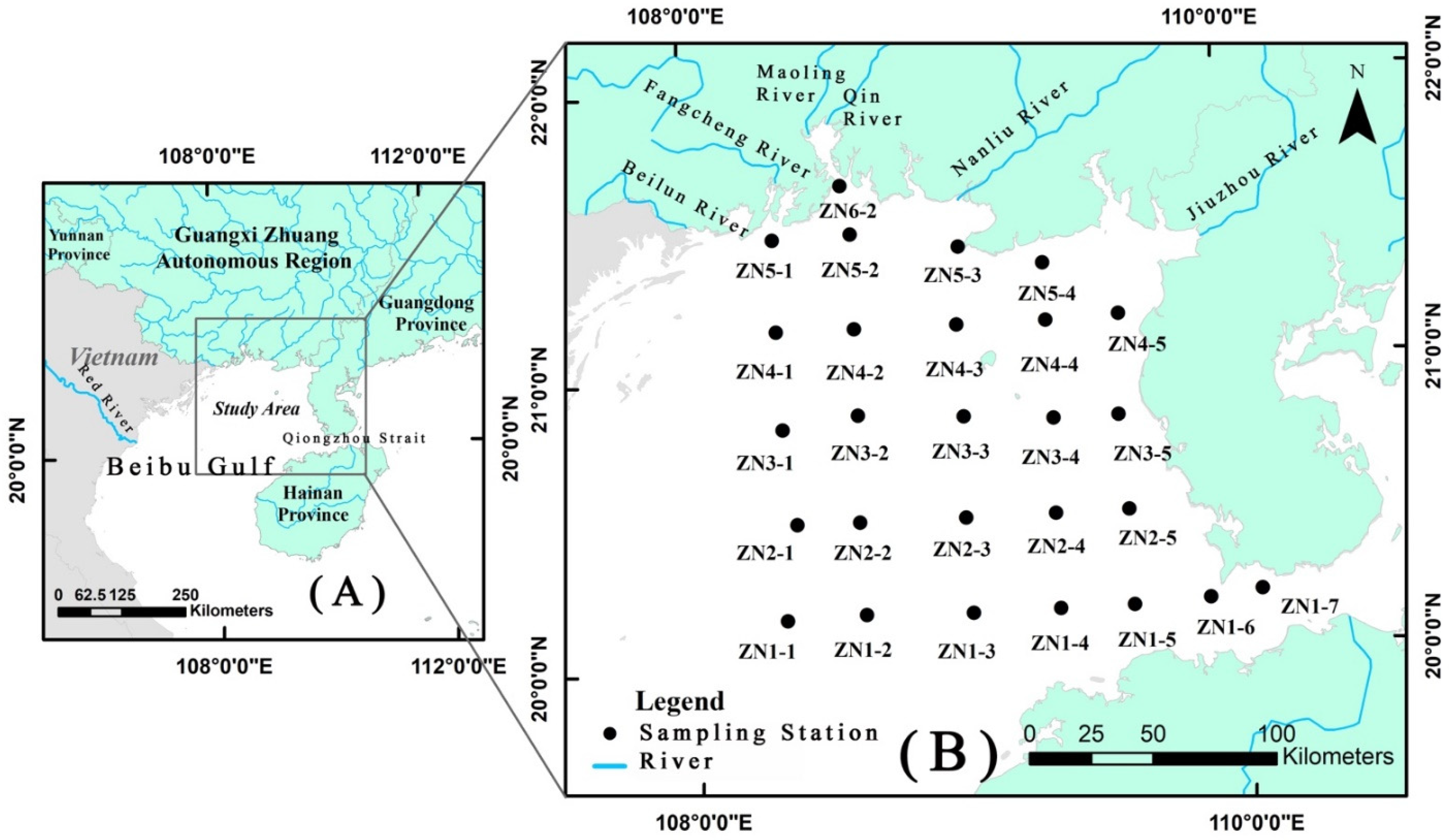
2.1. Sampling Strategy and Physico-Chemical Variables

Four oceanographic cruises were conducted in November, January, February, and April from 2018 to 2019 in the northern Beibu Gulf of China. Twenty-seven sampling stations were selected (Table 1 and Figure 1). SW (1 m depth) and BW (2 m above the seabed) samples were collected at stations deeper than 5 m. Only SW samples were collected from stations shallower than 5 m. In total, 213 phytoplankton samples were collected in the four cruises (Table 2). For each sample, 5 cm3 seawater was collected in a freezing tube, and 50 μL glutaraldehyde was added; then the samples were shaken and stored in liquid nitrogen until phytoplankton analysis by CytoSense flow cytometer. The seawater (500 cm3) used for nutrient analysis was filtered through a 0.45-μm cellulose acetate filter, which had been immersed in 1% hydrochloric acid solution for 12 h and washed with double distilled water. The filtered seawater samples were frozen at −20 °C until analysis. Nutrients dissolved in the water were determined in accordance with the method specified in the Specification of Oceanographic Survey [33], which is approved by the environmental protection department and is used extensively in China [34,35,36]. SiO3-Si, PO4-P, NO2-N, NO3-N, and NH4-N were analyzed with the silicon-molybdenum blue spectrophotometric method; ascorbic acid reduction phospho-molybdenum blue spectrophotometric method; diazo azo method; chrome-plating Zinc reduction-diazo azo method, and sodium hypobromate oxidation-diazo azo method, respectively. The limits of detection were 0.05 μmol L−1 for NO3-N, 0.02 μmol L−1 for NO2-N, 0.03 μmol L−1 for NH4-N, 0.02 μmol L−1 for PO4-P, and 0.10 μmol L−1 for SiO3-Si. Protocols used for nutrient detection are described below:
Twenty five centimeters cubed water used for SiO3-Si concentration detection is added to a conical flask containing 10 cm3 ammonium molybdate (8.0 g dm−3 )-hydrochloric acid mixed solution (2.4% volume fraction l), to form silicon molybdenum yellow complex, which is later reduced by 15cm3 p-methylaminophenol sulfate (20 g dm−3)-sodium sulfite (12 g dm−3) mixed solution. Silicomolybdenum blue complex is formed, and the absorbance is checked with a spectrophotometer at 812 nm. SiO3-Si concentration in sea water is calculated using the corresponding standard curve.
Twenty five centimeters cubed water used for PO4-P concentration detection is added to a conical flask, then reacted with 2.0 cm3 sulfuric acid (17% volume fraction)-ammonium molybdate (30.0 g dm−3)-antimony potassium tartrate (1.4 g dm−3) mixed solution (10:4:2, volume ratio), to form phosphorus molybdenum yellow complex. The yellow complex is later reduced by 0.5 cm3 ascorbic acid (54.0 g dm−3). Phosphorus molybdenum blue complex is formed, and the absorbance is checked with a spectrophotometer at 882 nm. PO4-P concentration in sea water is calculated using the corresponding standard curve.
Twenty five centimeters cubed water used for NO2-N concentration detection is added to a conical flask, then reacted with 0.5 cm3 1-naphthoethylene diamine dihydrochloride (1.0 g dm−3). Red color azo dye solution is formed, and the absorbance is checked with a spectrophotometer at 543 nm. NO2-N concentration in sea water is calculated using the corresponding standard curve. NO3-N dissolved in the water is reduced using a chrome-plated zinc sheet, to form NO2-N. Total NO2-N is analyzed using the method described previously. NO3-N concentration in sea water is obtained by subtracting the initial concentration of NO2-N. NH4-N in the water (25.0 cm3) is oxidized into NO2-N by potassium bromate (28 mg dm−3)- potassium bromide (20 mg dm−3)-hydrochloric acid (3% volume fraction)-sodium hydroxide (200 g dm−3) mixed solution. Total NO2-N is analyzed using the method described previously. NH4-N concentration in sea water is obtained after subtracting the initial NO2-N concentration.
Dissolved inorganic nitrogen (DIN) was calculated as the sum of the concentrations of NO3-N, NO2-N, and NH4-N; dissolved inorganic phosphorus (DIP) as PO4-P; and dissolved silicate as SiO3-Si. The equation for calculating DIN concentration is as follows [34,37,38]:
C(DIN) = C(NO3-N) + C(NO2-N) + C(NH4-N)
where C(DIN), C(NO3-N), C(NO2-N), and C(NH4-N) are DIN, NO3-N, NO2-N, and NH4-N concentrations, respectively.
The seawater temperature (T), salinity (S), and depth were measured using a Seabird SBE 911 plus CTD probe.
P. globasa colonies were collected using a 40-cm diameter plankton net with a mesh size of 500 μm. Colonies were collected from close to the seafloor to the surface. The volume of the water column passing through the net mouth was recorded using a HYDRO-BIOS D-Flow digital flow meter (HYDRO-BIOS, Alternholz, Germany) tied to the net mouth. Colonies were observed and counted under a stereomicroscope (SMZ-800, Nickon, Japan). Colony concentrations along the entire water column were calculated at each station.

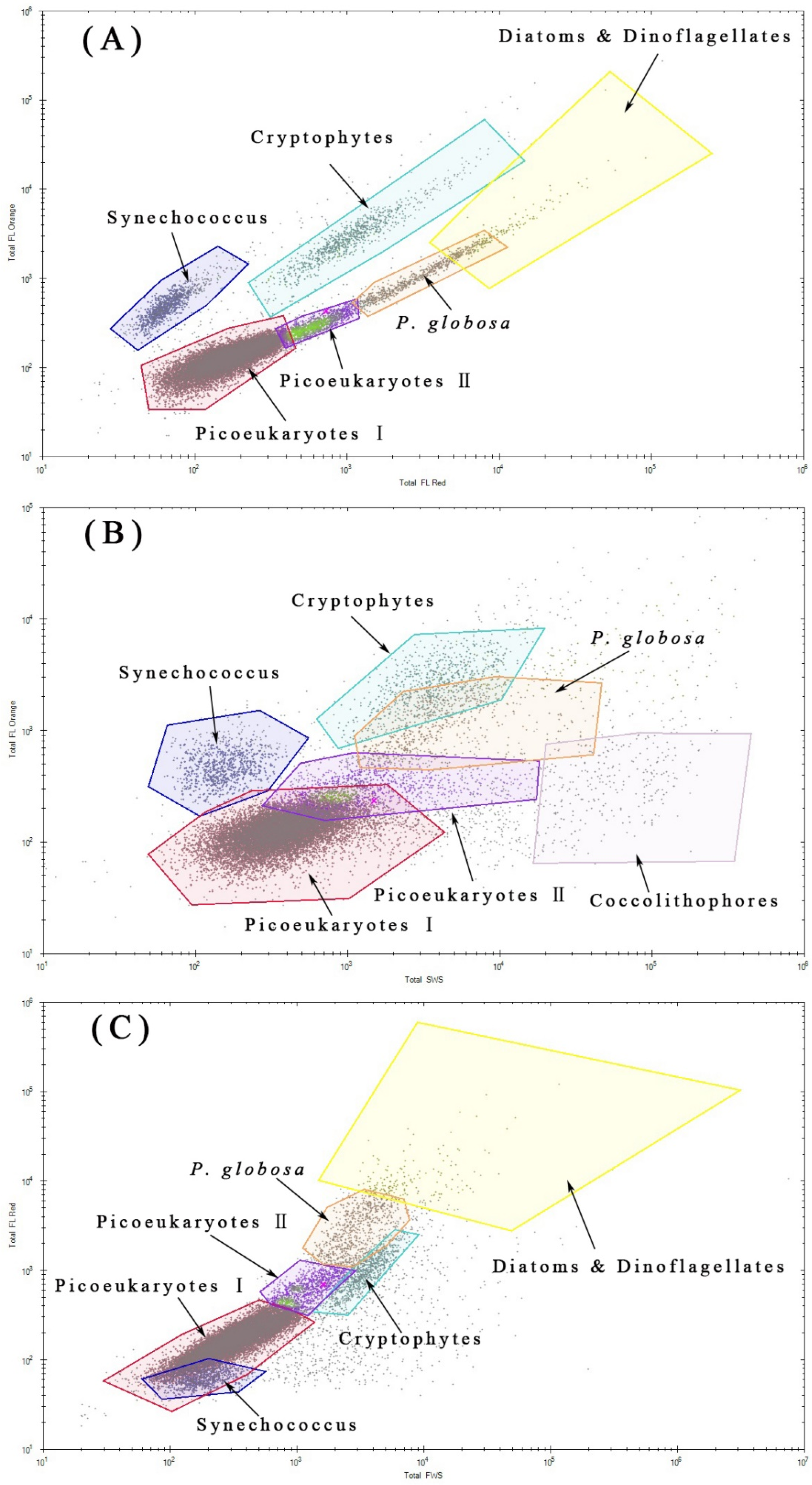
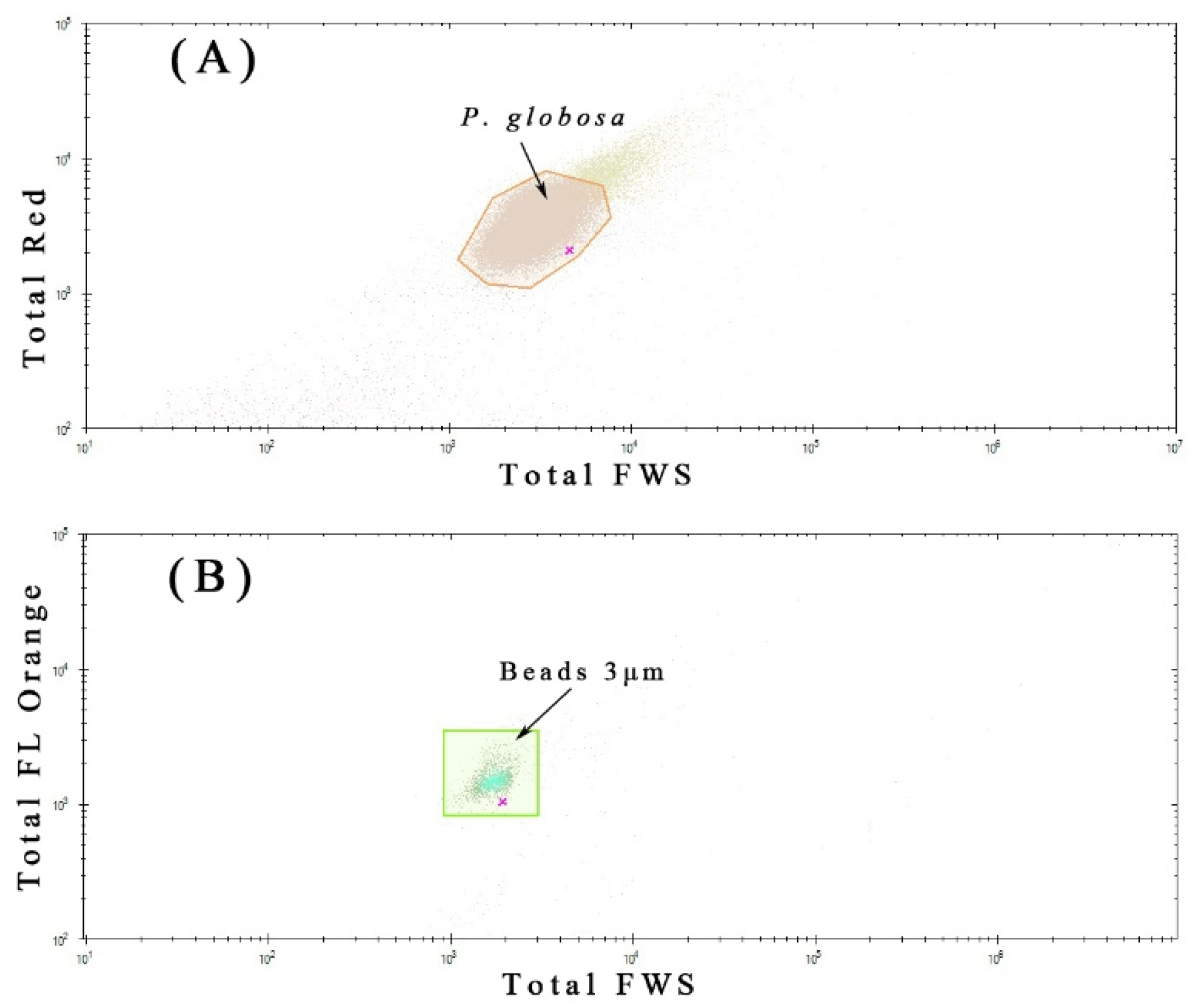
2.2. Phytoplankton Discrimination by Flow Cytometry

Samples stored in liquid nitrogen were defrosted and analyzed using a Cytosense pulse-shape recording flow cytometer (Cytobuoy© b.v., Johan de Wittlaan, The Netherlands). Sheath fluid was used to separate, align, and drive the particles into the laser. The flow rate was 5.0 μL s−1. Single cells and colonies were discriminated using a laser beam (excitation wavelength 488 nm, 50 mV), and a 10-mv red fluorescence trigger lever was set. Each analysis lasted for 4 min. The mean volume analyzed was 1.28 ± 0.11 cm3. The CytoSense instrument was equipped with an optional module of ‘high-sensitivity’ photomultiplier tubes, to differentiate picophytoplankton and provide reliable counts [28]. The stability of the optical unit and size calibration was checked using a PE Calibration Particle Kit (SPHEROTM, Spherotech Inc., Lake Forest, IL, USA; 3.1 μm in diameter).
Samples were analyzed using CytoClus4© software (V4.8.2.8, Cytobuoy© b.v., Johan de Wittlaan, The Netherlands, https://www.cytobuoy.com/product/software/). Clusters were manually classified according to the amplitude and shape of the five optical signals characterizing each particle: forward scatter (FWS), sideward scatter (SWS), and three fluorescence signals collected by photomultiplier tubes (red (FLR, 668–734 nm), orange (FLO, 601–668 nm), and yellow (FLY, 536–601)). Mathematical variables were assigned to each signal shape: inertia, fill factor, asymmetry, number of peaks, length, and apparent size. All these values were plotted onto various two-dimensional cytograms of retrieved information from the five pulse shapes obtained for each single cell, mainly the integral (total signal) and peak of the pulse-shape signal (maximum height). Once phytoplankton cells had passed through the laser beam of the flow cytometer, red fluorescence was generated from chlorophyll-a in microalgae. The red fluorescence triggered the FCM detector and was recorded by the flow cytometer as one event. FCM counted all events, as well as the volume of the analyzed sample, and the phytoplankton abundance in each sample was determined.
Based on previous CytoSense FCM studies [28,29,39,40], seven phytoplankton clusters were identified in the present study (Figure 2). Diatoms and dinoflagellates showed the highest FLR and FWS signals because of their large size and high chlorophyll-a content. Phaeocystis globosa solitary cells were characterized by lower FLR and FWS signals compared with those of microphytoplankton groups. To confirm the optical signal fingerprint of this group, we analyzed the pure culture of this species using FCM and defined its clusters (Figure 3A). Picoeukaryotes are the smallest eukaryotic cells, and they showed lower FLR and FWS signals compared with those of P. globosa. Picoeukaryote II showed a higher FLR signal compared with that of Picoeukaryotes I, indicating higher chlorophyll-a content. The Synechococcus cluster showed a distinct signature because of its small size and a peak in orange fluorescence caused by high phycoerythrin content [29]. Cryptophytes had higher FLO and FWS signals compared with those of Synechococcus, owing to their larger size and higher phycoerythrin content per cell. Coccolithophores were high in the SWS signal owing to their CaCO3 platelet coverage. Zhao et al. identified Prochlorococcus using traditional FCM [32]. However, there was little evidence for the presence of this group in samples collected during our four cruises. The fluorescence signals produced by these small cells (mean cell size 0.6 μm) were so low that they were hardly differentiated from baseline fluorescence noise. According to previous studies, Prochlorococcus are preferentially distributed in ocean waters rather than coastal waters [41,42].

2.3. Data Treatments and Analysis

The significant differences between water T, S, nutrients, and phytoplankton abundance from different cruises and different layers were tested using a one-tailed t-test performed using SPSS22.0. The line charts reflecting the mean value trends of physicochemical factors and phytoplankton abundance from the four cruises were drawn with SigmaPlot 14.0, as were the stacked bars of the phytoplankton groups. A horizontal distribution chart of the physiochemical factor values and phytoplankton abundance was plotted using Golden Surfer 13.0. To analyze the relationship between environmental parameters and phytoplankton communities, redundancy analysis (RDA) was performed using Canoco 4.5 software [43,44,45,46]. Before that, a detrended correspondence analysis of the species data was employed to determine whether linear or unimodal ordination methods should be applied. The abundance of each phytoplankton group and environmental factors were log(x + 1) transformed, to minimize the influence of extremely high or low values and to ensure a normal distribution.

3. Results

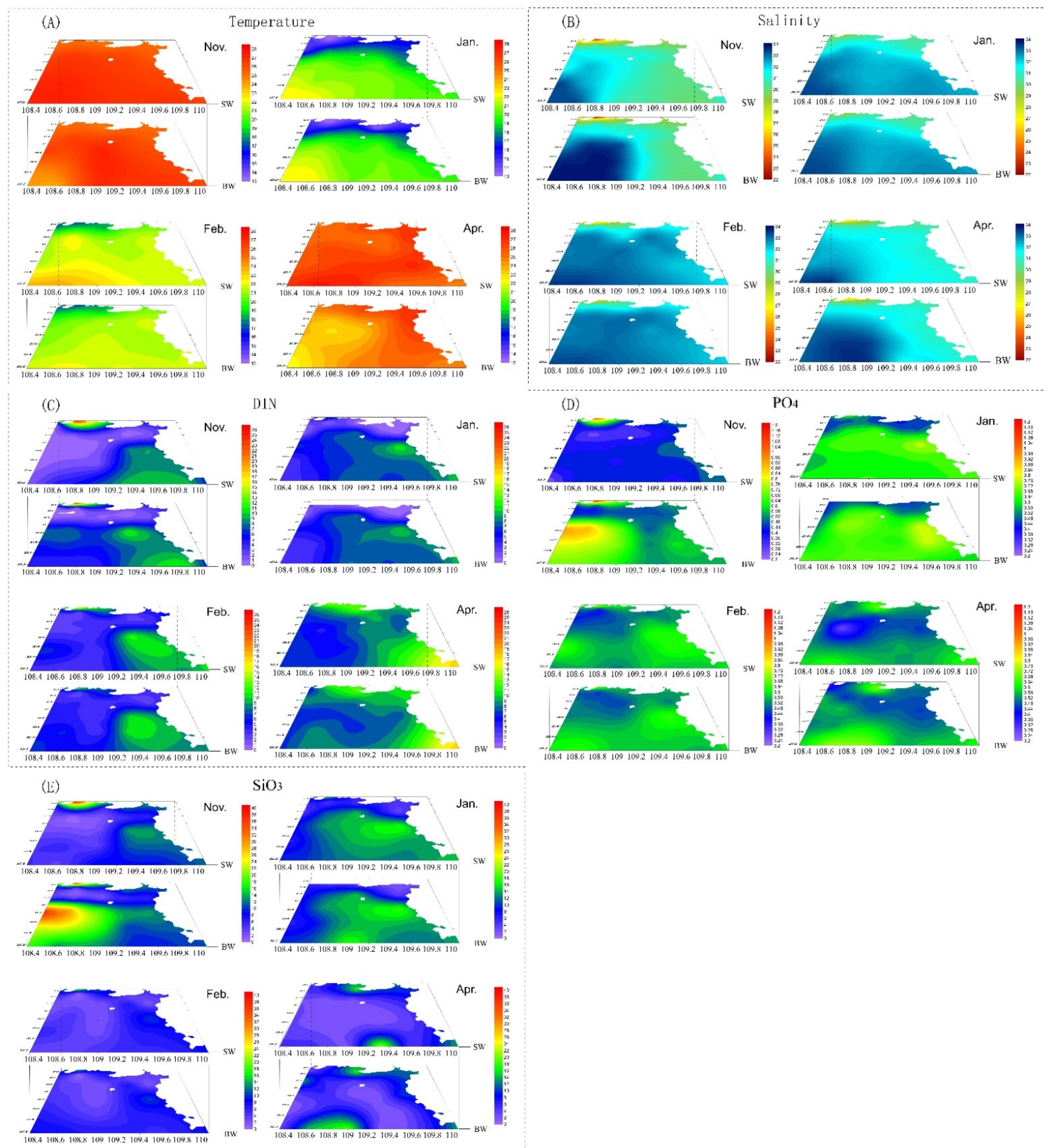
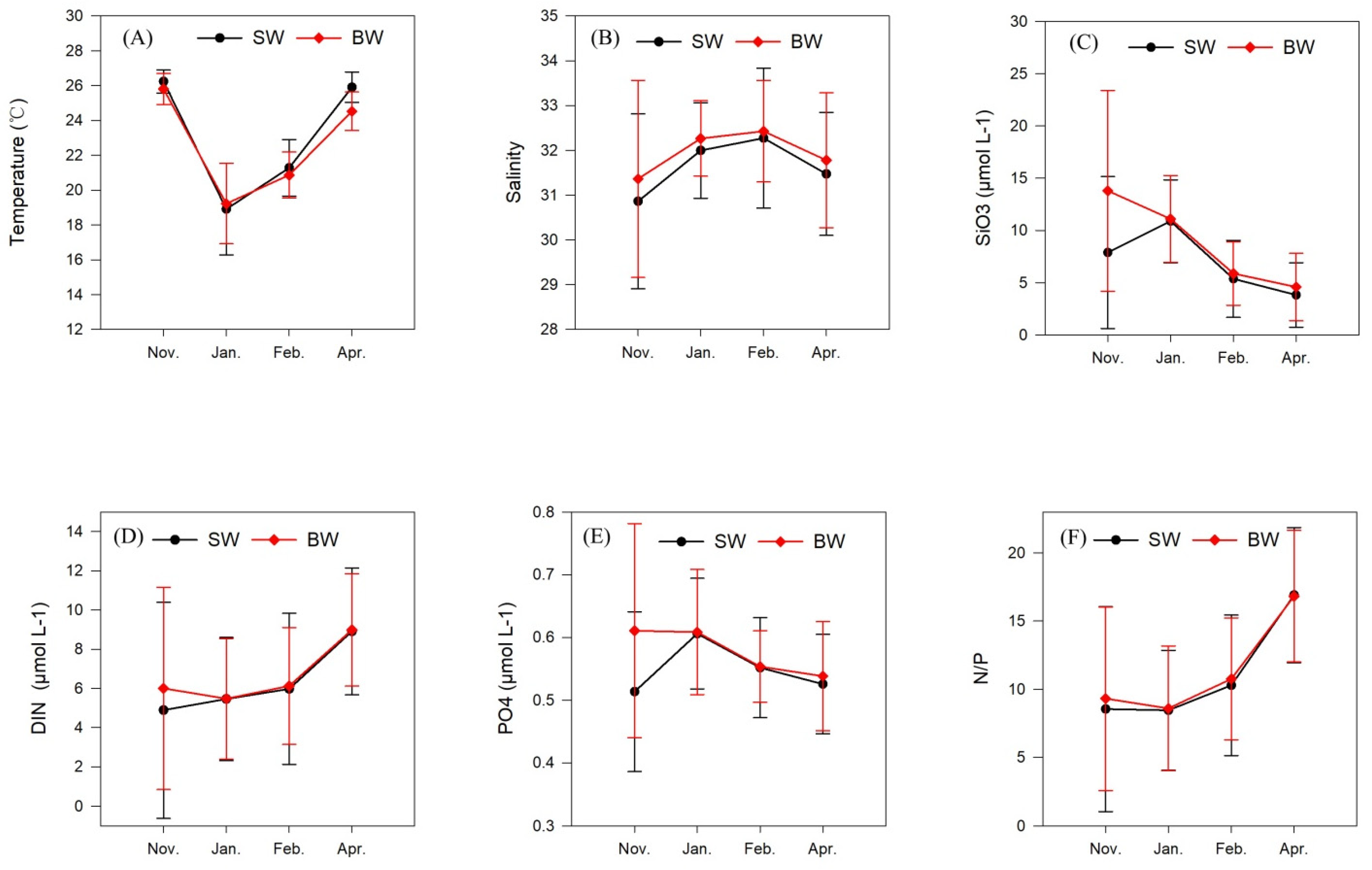
3.1. Temperature and Salinity

The spatiotemporal variations in T and S are shown in Table 3 and Figure 4, respectively. The variation trends of these two factors are shown in Figure 5. During the four cruises, surface seawater temperature (SST) and bottom seawater temperature (BST) ranged from 13.01 °C to 27.73 °C. Water T decreased sharply from November to January and increased from January to April. SST was lower than BST in January, whereas it was higher during the other three cruises. The SST and BST remained high throughout the region in late autumn (November). A low-BST area was observed in the southwest corner. In winter, the water was affected by the cold northeast monsoon, and the T was low in the north coastal area, increasing gradually from north to south. Water T was homogeneous in the vertical direction in January. In spring, as the monsoon weakened, SST increased due to solar radiation. The BST remained low in the southwestern area in April.
The mean S was lowest in November, after which it increased, peaking in February (Table 3, Figure 5). The S ranged from 22.80 (station ZN6-1, SW, November) to 33.81 (station ZN1-5, BW, November) with a mean value of 31.80. In general, the high-S mass was in the southwest region, whereas the low-S mass was distributed along the coastal region. There was mixed shelf water between them.

3.2. Nutrients

The spatiotemporal variation in nutrients is shown in Table 3, Figure 4 and Figure 5. Figure 4C and Figure 5D show the distribution and variation trend of DIN. In November, the mean concentration of DIN was 5.46 ± 5.31 μmol L−1, ranging from 0.53 to 25.42 μmol L−1. The concentration of DIN in the SW was 6.00 ± 5.05 μmol L−1, which was higher than that in the BW. In January, the DIN concentration in SW increased, whereas that in BW decreased. DIN concentrations in both SW and BW slightly increased in February and then continued to increase sharply in April, reaching 8.91 ± 3.18 μmol L−1 and 8.99 ± 2.81 μmol L−1, respectively. In November and April, the high-concentration region was at Qinzhou Bay and Qiongzhou Strait, north and southeast of the study area, respectively. In January and February, high DIN was distributed along the Leizhou Peninsula coast east of the investigated area.
Figure 5D shows the variation trend of PO4 during the four cruises. In November, the mean PO4 concentration of BW was 0.61 ± 0.17 μmol L−1, which was significantly higher than that of SW (p < 0.05). In January, the PO4 of BW remained almost the same as that in November, while the PO4 of SW decreased to 0.61 ± 0.09 μmol L−1. The PO4 concentration in both the SW and BW decreased in February and remained relatively low in April. The spatial distributions of PO4 concentration in the four cruises are shown in Figure 4E. The vertical distribution of PO4 was heterogeneous in November. On the surface, it was high in the northwestern coastal area. At the bottom, in addition to that in the northeast coastal area, there was another area of high PO4 concentration in the west, which became homogenous in January with a vertical distribution. The highest concentration was observed in the eastern coastal area. All regions from middle to south contained relatively high PO4 in January. In February, the eastern and southwestern parts still had the highest PO4 concentrations. In April, Lianzhou Bay, which lies in the north coastal area, had the highest PO4 concentration, while that of the southeast and southwest remained high.
The spatiotemporal distribution of SiO3 (Figure 4E and Figure 5D) was similar to that of PO4. In November, the mean concentration of BW was 9.43 ± 9.43 μmol L−1, which was higher than that of SW (p < 0.05). There was an area with evidently high SiO3 concentration in the western part, similar to the PO4 distribution, and it became homogeneous in January. The SiO3 concentration in both SW and BW decreased from January to April. The mean SiO3 concentration was 5.63 ± 3.09 μmol L−1 and 4.20 ± 3.16 μmol L−1 in February and April, respectively.

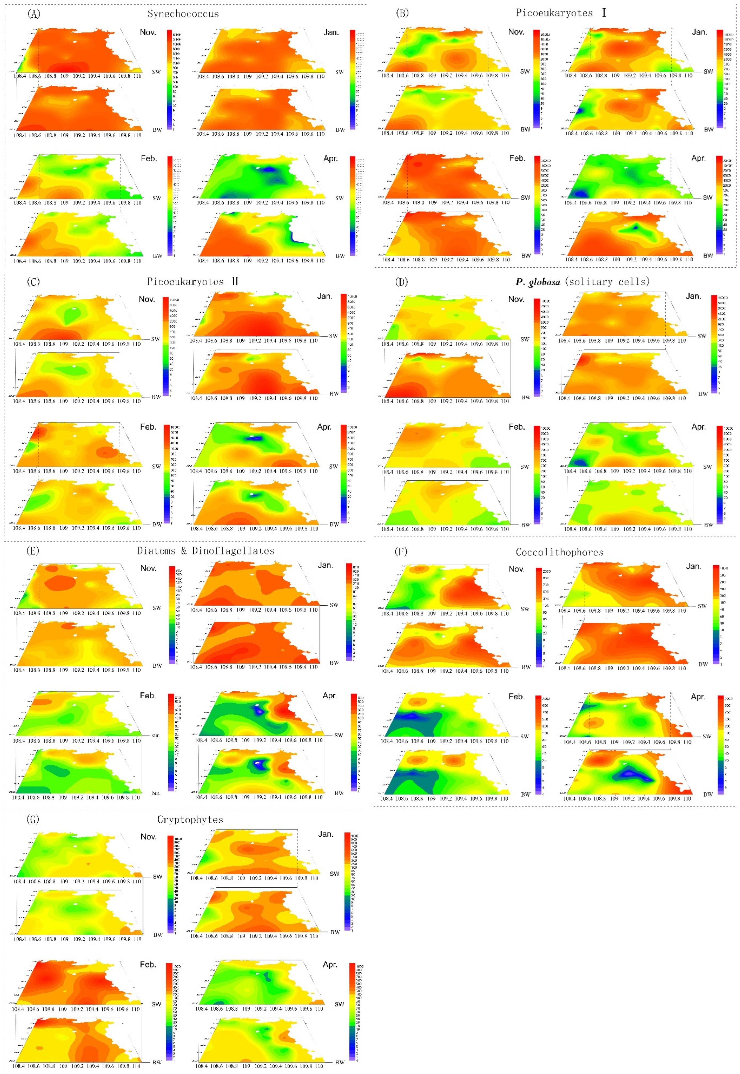
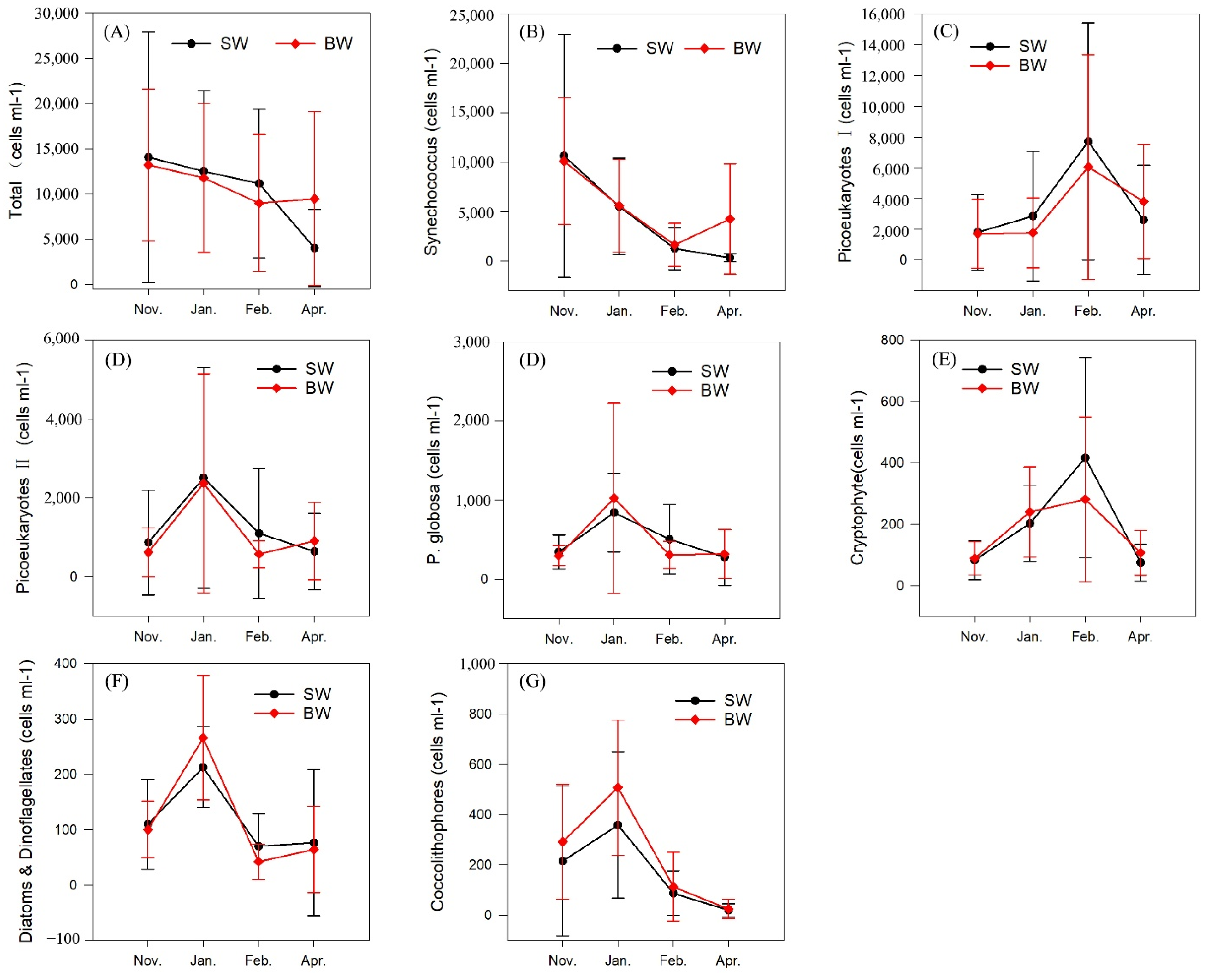
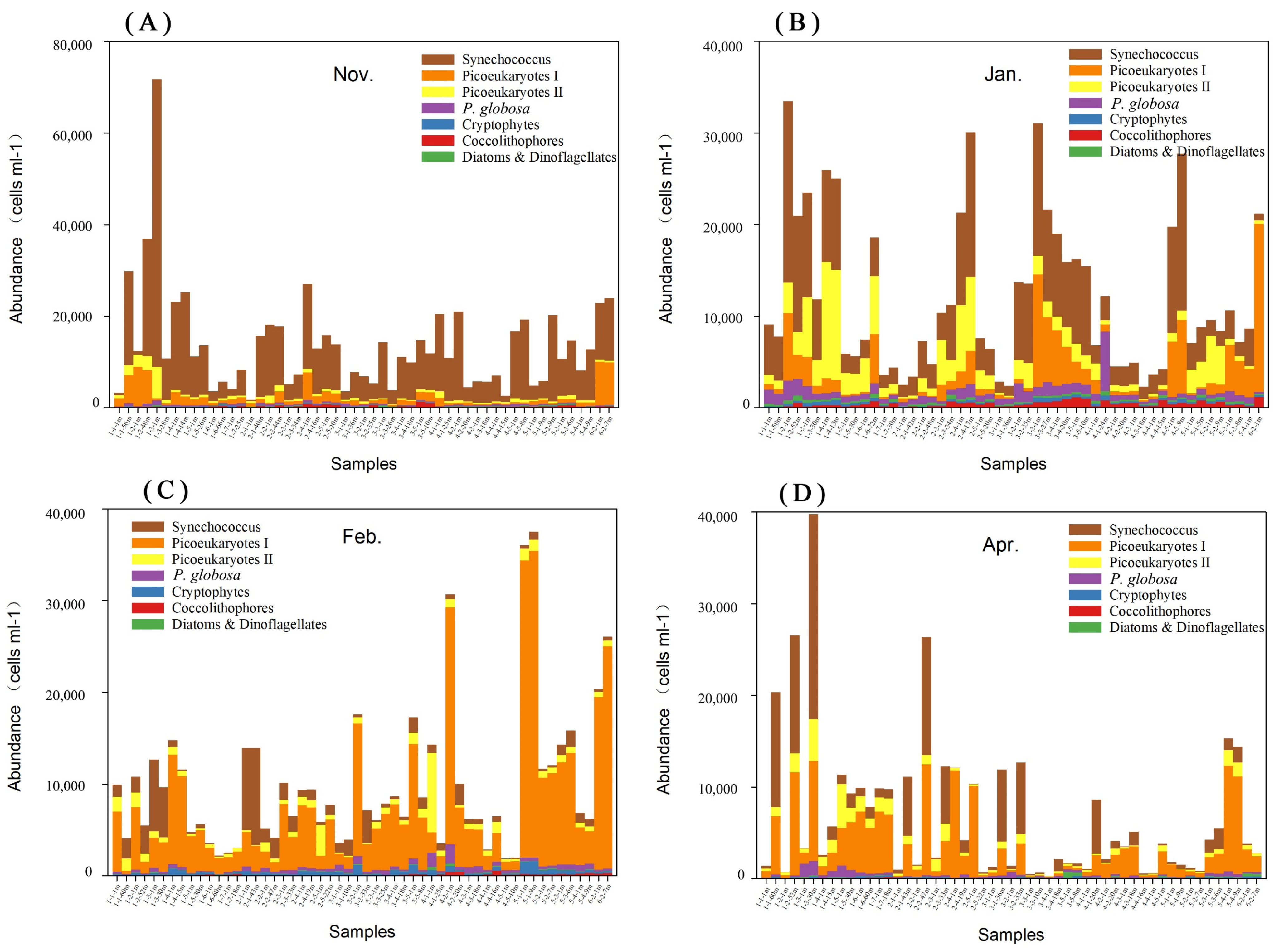
3.3. Phytoplankton Composition and Spatial and Temporal Patterns

In the north of the Beibu Gulf between November 2018 and April 2019, seven phytoplankton clusters were present on all dates and in all stations, as determined using FCM. The spatiotemporal variation of phytoplankton groups is shown in Table 4, Figure 6 and Figure 7. Synechococcus, Picoeukaryote I, and Picoeukaryote II were the dominant groups throughout the study period (Figure 8). These accounted for 47%, 32%, and 11% of the total phytoplankton abundance, respectively. Phaeocystis globosa accounted for 5%, and cryptophytes, diatoms, dinoflagellates, and coccolithophores accounted for the remaining 5%.
Synechococcus abundance decreased from November to February and then again in April. The average abundance of this group was 5.0 × 10³ cells mL−1, and the maximum was 6.3 × 10⁴ cells mL−1 (station ZN1-3, surface, November). Contrary to the variation trend in Synechococcus, Picoeukaryote I and Cryptophyte abundance was high in February, peaking at 3.3 × 10⁴ cells mL−1 (station ZN5-1, bottom) and 1.4 × 10³ cells mL−1 (station ZN5-1, bottom), respectively. Picoeukaryote II, P. globosa, diatoms and dinoflagellates, and coccolithophores showed similar variation trends; they were high in January and then decreased in February, remaining low in April.
In terms of horizontal distribution, Synechococcus was more abundant in offshore waters during the four cruises. The vertical distribution was homogeneous in January and February and heterogeneous in April. BW abundance was significantly higher than SW abundance (p < 0.05) in April.
Picoeukaryote I abundance was high in the northern and southern regions in November, and this high abundance spread to the central area. The abundance continued to increase in February, and in April, the abundance decreased in SW but remained high in BW.
Picoeukaryote II abundance peaked in the south–southwestern area in November. The high-abundance areas were located in the northwest and middle to south in January. The distribution in February was similar to that in January, but the mean abundance was lower than that in January. Picoeukaryote II was highly abundant in the south and northeastern areas in April.
The vertical distribution of solitary P. globosa cells was heterogeneous in November, with a higher abundance in BW compared with that in SW. The maximum abundance was observed in the southwestern region (station ZN4-1, BW), reaching 6.5 × 10³ cells mL−1. In January, the abundance became more homogeneous. In February, P. globosa in SW were highly abundant in the northwestern area, while P. globosa in BW were highly abundant in the northern area. In April, high abundance was observed in the northern, western, and southern areas.
The horizontal distribution of diatoms and dinoflagellates showed no evident regularity. In November, the abundance of diatoms and dinoflagellates in SW was high in the northwest and central areas (southwest of Weizhou Island), and their abundance in BW was high in the north near Lianzhou Bay. In January, their abundance in SW was high in the northwestern, eastern, southeastern, and southwestern areas, while their abundance in BW was high in most areas. In April, diatoms and dinoflagellates were highly abundant in the nearshore areas.
Coccolithophore abundance was high in nearshore areas during three of the cruises, except for January when the abundance was high in most areas. The distribution of cryptophytes showed no clear regularity. The maximum abundance of this group was observed at station ZN5-1 BW in February, reaching 1.42 × 10³ cells mL−1.

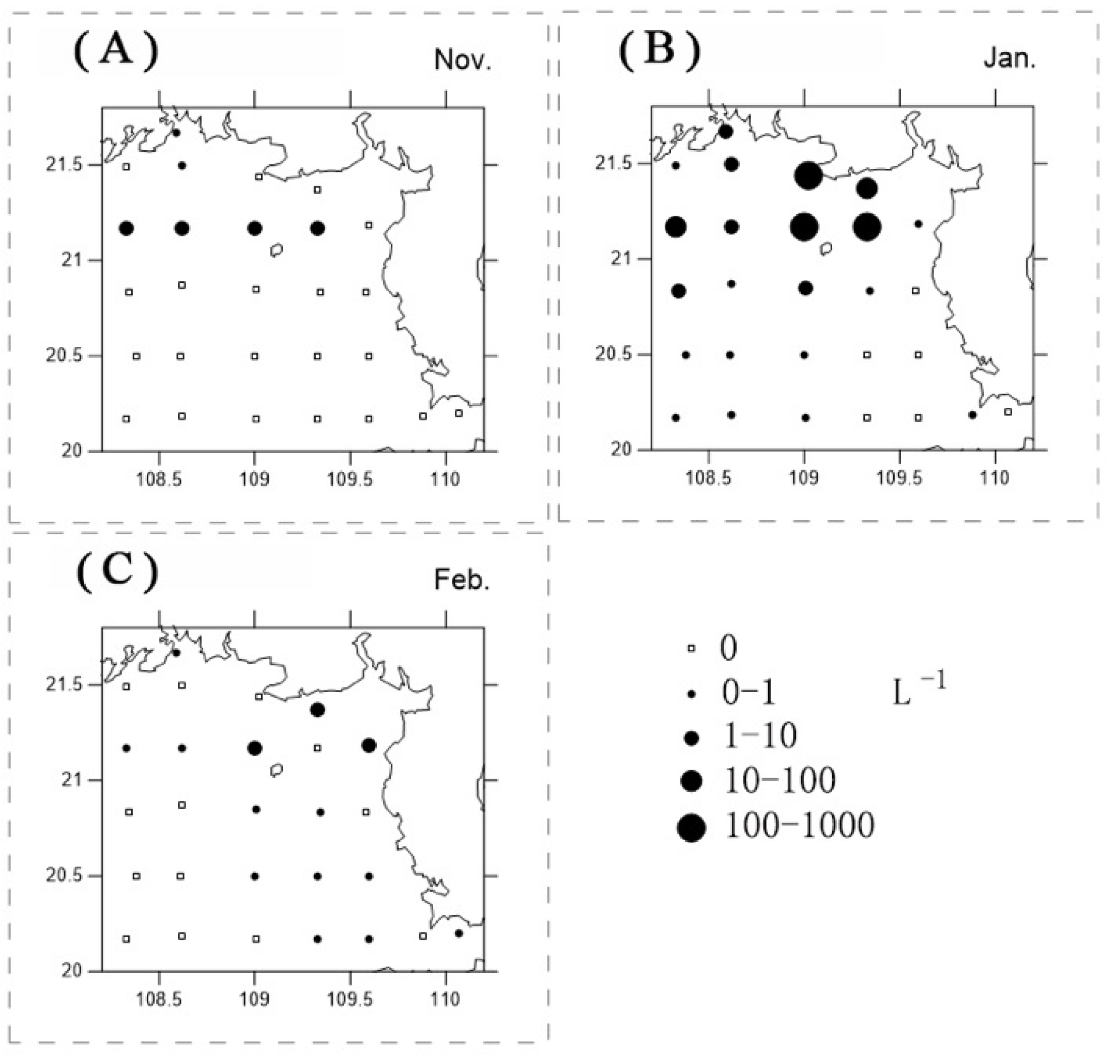
3.4. Phaeocystis Globosa Colonies
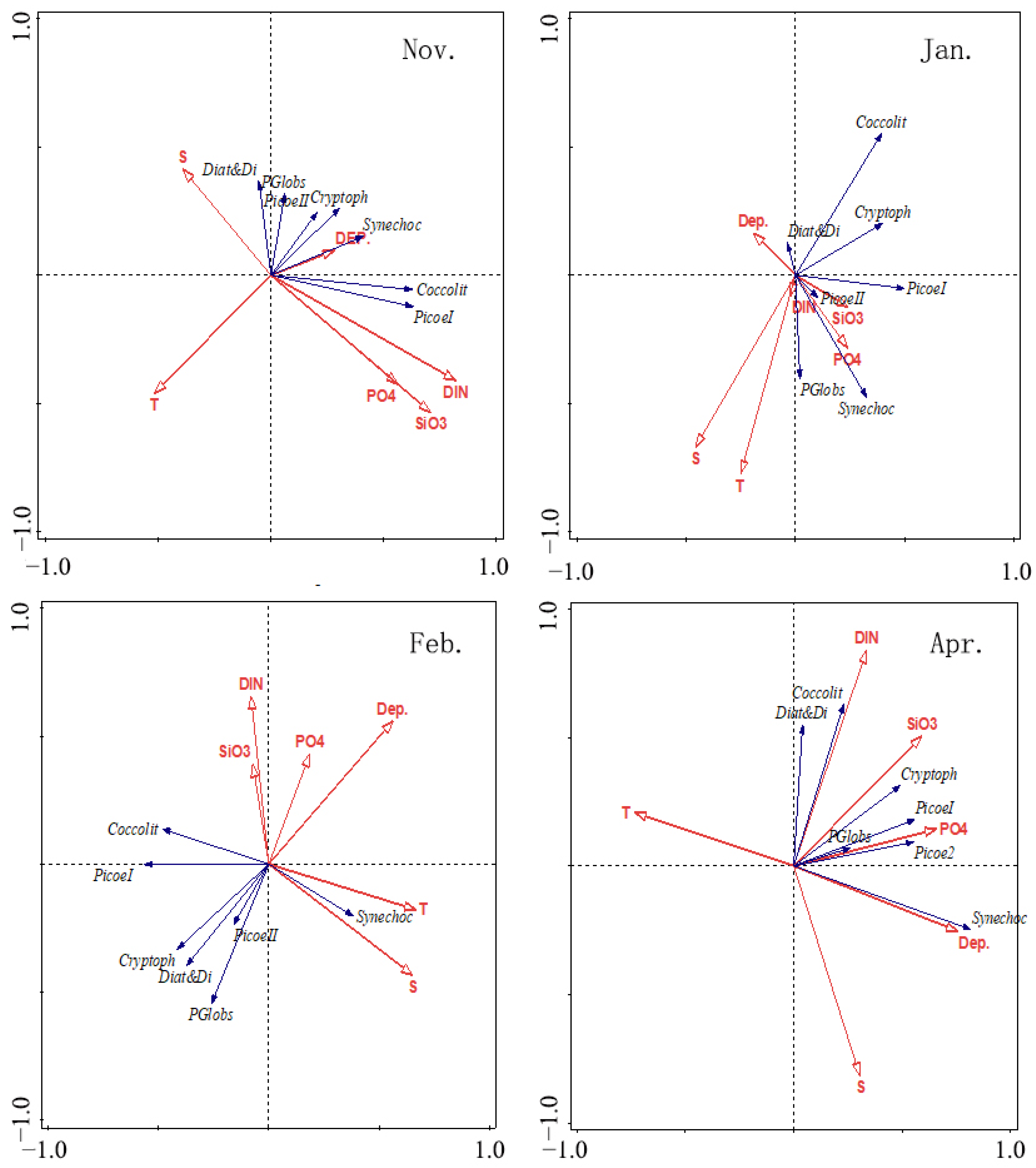
P. globosa colonies from each station were counted. As shown in Figure 9, colonies were found at six stations in November, 21 stations in January, and 14 stations in February. No colonies were observed in April (data not shown). The highest colony abundances were 2.7 L−1 in November (station ZN4-3), 189.8 L−1 in January(station ZN4-4), and 9.4 L−1 in February (station ZN5-4).

3.5. RDA Results

To analyze the relationships between environmental factors and phytoplankton assemblages, and to understand the driving factors that control phytoplankton community structure, redundancy analysis (RDA) was performed.
In November, the eigenvalues of axes 1 and 2 were 0.225 and 0.039, respectively (Table 5). The correlation values for axes 1 and 2 were 0.80 and 0.43, respectively, indicating that the correlation between axis 1 and phytoplankton taxa was significantly positive (r ≤ 0.8) and that between axis 2 and phytoplankton taxa was weakly positive (0.3 < r < 0.8). The cumulative value of the explained fitted variation was 86.1%, which meant that the first two axes explained 86.1% of the taxa–environment relationship. The results from the other three cruises are listed in Table 5.
Table 6 and Figure 10 show the relationships between the phytoplankton taxa and environmental variables. The main environmental factors influencing the phytoplankton community were DIN and T in November (p < 0.05), S, SiO3, DIN, and T in January (p < 0.05), T, depth, and PO4 in February (p < 0.05), and depth, DIN, and PO4 in April (p < 0.05).

4. Discussion

4.1. Hydrology

Previous studies have shown that there are three main water masses in the Beibu Gulf: coastal water (CW) with low salinity, bottom shelf water (BSW) with low temperature and high salinity, and mixed shelf water (MSW) [47,48]. The MSW can be further divided into two types, depending on whether it flows from the Qiongzhou Strait or the South China Sea [49]. In November (late autumn), the BSW was distributed in the southwest, the CW was distributed along the Guangxi coast in the northern area, and the MSW was spread over the rest of the area. In January, the water temperature in the northern area dropped sharply because it was affected by the cold northerly wind. A strong northeast monsoon in winter transports cold water from the sea surface to the bottom [48], resulting in homogeneous temperature and salinity in the vertical distribution (Figure 4A,B). In February, the water temperature was similar to that in January except at stations that were investigated in daylight, which had a higher surface temperature than the adjacent stations. The MSW was widely distributed in the investigated area, but the CW was restricted to the southwestern corner. In April (spring), the cold water mass remained in the bottom layer as the thermocline strengthened, while in the shallow water, the thermocline was broken by strong tidal mixing [48].

4.2. Nutrients Spatiotemporal Distribution and Sources

Runoff from the Guangxi coast replenishes nutrients in the sea area. In November, the SW nutrients showed the highest concentrations in the northern coastal area, and nutrient distribution was highly influenced by input from the Qin and Maoling rivers. Another high-nutrient area was observed in the SW in west. Yuan et al. reported a nutrient concentration hotspot in the same area in December 2016 [36]. We deduced that this area was affected by discharge from the Red River. The Red River estuary lies 110 km west of the investigated area, and the discharge from this river in Hanoi (Red River Delta) was approximately 1000 m3 S−1 in November. The mean phosphate and dissolved Si concentrations at that river delta were 0.15 mg P L−1 (4.8 μmol L−1) and 4.5 mg Si L−1 (160.7 μmol L−1), respectively [50]. This high level of discharge from the Red River coupled with high nutrient content running into the Beibu Gulf greatly affected the nutrients in the seawater. Shi et al. [51] observed anticyclonic circulation northwest of the Beibu Gulf, which could carry the nutrients from the Red River to the northeastern region. In our study, we observed a low-salinity region in the south (Figure 4B). This is another trace of the Red River plume.
In winter, freshwater discharge carries the lowest levels of nutrients observed throughout the year [52]. Nutrients became homogeneous under the influence of the northeast monsoon. In January and February, the nutrient concentrations in the SW and BW at the same station were nearly the same. High DIN concentrations spread from the northeast to east and were affected by the discharge from the Pearl River being transported through the Qiongzhou Strait. The water from the Qiongzhou Strait became the major factor affecting the spatial distribution of nutrients, primarily during the winter–spring period. According to Shi et al., the mean outflow of water in winter–spring is higher than that in summer–autumn (0.2–0.4 Sv (Sv = 106 m3 S−1) and 0.1–0.2 Sv, respectively) [1]. Gao et al. reported that the mean westward flux is ~0.35 Sv in autumn and winter [47], which is consistent with the findings of Shi et al. [1]. Zhang et al. estimated that the DIP westward through the Qiongzhou Strait into the Beibu Gulf in winter accounts for 54% of throughout the year [34,53]. In addition to the high-value area in the Qiongzhou Strait, there was another hotspot of PO4 and SiO3 concentrations in the south. This hotspot indicated that PO4 and SiO3 were also affected by the BSW from the South China Sea. The Red River plume weakened during winter when the runoff decreased [47]. Meanwhile, the northwest monsoon pushed the Red River water mass to the south. These were the two factors leading to the decline in the Red River’s influence on this region. The SiO3 concentration decreased significantly from January to February. This was probably due to the sharp increase in diatoms and dinoflagellates in January, which consumed the Si, leading to the depletion of SiO3 in February.
Rainfall increased in spring, which is also when fertilizer use increases for spring plowing. Thus, areas of high DIN and PO4 concentrations spread out along the northern coastal zone of Guangxi. The Qiongzhou Strait in the southeast had the highest concentrations. The influence of the BSW from the South China Sea remained, but was weakened. The DIN abundance was the highest in February among the four cruises. PO4 flowed through the Qiongzhou Strait into the Beibu Gulf and declined in spring (Figure 4D). Zhang et al. reported that the SRP westward through the Qiongzhou Strait into the Beibu Gulf in spring only accounted for 18% of the annual amount (54% in winter) [53].

4.3. Phytoplankton Abundance and Composition

Zhao et al. investigated pico- and nano-phytoplankton assemblages in the same area from September 2016 to August 2017, using FCM [32]. Four clusters were identified in their study, including picoeukaryotes, nanoeukaryotes, Synechococcus, and Prochlorococcus. Synechococcus and picoeukaryotes were also found in the present study. However, we separated picoeukaryotes into two groups, based on their sizes and chlorophyll-a contents. Nanoeukaryotes is a type of phytoplankton that has a 3–20-μm diameter range, which includes the P. globosa group and parts of other groups in the 3–20-μm diameter range, in the present study. Prochlorococcus was absent in the present study.
According to the research of Zhao et al., Synechococcus mean abundance peaked at 1.66 × 10⁵ cells mL−1 in August, and dropped to the lowest abundance, 3.65 × 10³ cells mL−1, in January. In the present study, the highest Synechococcus mean abundance was 1.04 × 10⁴ cells mL−1, in November; whereas the lowest mean abundance was 1.48 × 10³ cells mL−1, in February. The highest Synechococcus abundance in the present research being lower than that of Zhao et al., might have been due to the different sampling times. In Zhao et al.’s research, the highest picoeukaryote abundance was 5.56 × 10³ cells mL−1, in February, and the lowest was 1.02 × 10³ cells mL−1, in January. We combined the abundances of Picoeukaryotes I and Picoeukaryote II into total Picoeukaryotes abundance. The highest total Picoeukaryotes abundance was 7.51 × 10³ cells mL−1, in February, and the lowest was 2.49 × 10³ cells mL−1, in November. In conclusion, the phytoplankton abundance and trends in our research are similar to those of Zhao et al.

4.4. Relationships between Environmental Variables and Phytoplankton Assemblages

Synechococcus abundance decreased from November to February and then increased in April. RDA results indicated that, in November, the Synechococcus abundance was mainly related to nutrient concentration and depth. The depth is inversely related to irradiance to some extent. Previous studies have found that Synechococcus can grow under very low light levels and outcompete larger cells for nutrient uptake [28,29,54]. In January and February, Synechococcus was associated with a seasonal decrease in seawater temperature. This group is a tropical species and so was restricted by low temperatures. In April, when the seawater temperature increased, Synechococcus abundance was associated with nutrient level and depth. The temporal and spatial distributions of Picoeukaryote I were similar to those of Synechococcus. However, Picoeukaryote I was not related to water temperature, which was low in January and February. This meant that Picoeukaryote I could tolerate low water temperatures. Picoeukaryote II abundance increased from November to January, decreased sharply from January to February, and increased again from February to April. A similar trend was observed for diatoms, dinoflagellates, and P. globosa. The lack of PO4 could have resulted in a decrease in these three phytoplankton groups in February.
There were two reasons for the decrease in PO4 in February and April. The first was the increasing abundance of Picoeukaryote I, diatoms, dinoflagellates, and P. globosa. These three groups were more numerous than Synechococcus and Picoeukaryote I, and their large populations consumed large amounts of nutrients, which led to PO4 depletion. The second reason is that the amount of PO4 coming from the Qiongzhou Strait decreased at that time. Zhang et al. reported that the amount of PO4 originating from the Qiongzhou Strait in spring was only one-third of that in winter [53]. The PO4 concentration continued to decrease in April, leading to an increase in the DIN:DIP ratio. Phytoplankton proliferate rapidly at suitable N:P ratios [55]. According to previous studies, the growth of most red-tide-causative organisms in Hong Kong coastal waters is optimized at a low N:P (atomic) ratio of between 6 and 15 [56]. Although the water temperature and DIN increased in April, the PO4 concentration was low and the N:P ratio was high. The mean N:P was 8.5 and 16.9 in January and April, respectively. Phosphate was the primary limiting factor in the winter–spring period in the Beibu Gulf. This is why phytoplankton abundance either did not increase or only increased slightly from February to April. Other factors such as turbulence and predators could be the main structural drivers of spatiotemporal assemblage distribution [57,58]. However, these factors were not investigated in the present study.

4.5. P. globosa Solitary Cells and Colonies

There are two distinct forms in the life cycle of P. globosa: free-living cells and colonies, with each colony containing thousands of cells. Colony cells are without flagella (non-flagellates) and are fixed in a polysaccharide matrix, whereas free-living cells possess two flagella (flagellates). Non-flagellate and flagellate cell types alternate during the life cycle of P. globosa [11,12,59]. There are two sizes of flagellate cells: small (3.4–4.1 μm) and macroflagellate (5.6–8.3 μm) [22]. These cell types also differ in their chromosomal numbers, with small flagellates being haploid and macroflagellates being diploid [15]. Bonato et al. [28,29] distinguished between the two types of flagellates using FCM. Diploid macroflagellates showed higher FLR and FWS signals than small haploid flagellates. However, we were not able to differentiate them in the present study. Previous studies have suggested that macroflagellates have a short lifetime (less than a day), which explains why this flagellate stage is rarely observed [10,12]. Therefore, free-living P. globosa cells were not divided into their two types in the present study and were considered together as solitary cells.
Flagellates are generated inside fading colonies, and many flagellates are released when P. globosa blooms fade [10,12,60]. Peperzak et al. found that the relative concentration of solitary cells peaked 17 and 7 days after the peaks of non-flagellate cells (colony cells) [22]. In the present study, P. globosa colonies peaked in January, decreased in February, and were rarely found in April. Solitary cells peaked in January and were maintained at similar levels in November, February, and April. The number of P. globosa colonies decreased from January to April, but the number of solitary cells did not increase. The maximal colony abundance was just 189.8 L−1, which was lower than that of other blooms. Hai et al. reported a maximal colony abundance of 2200 L−1 [61]. It is possible that colony abundance would peak at a certain moment between November and January. Although abundance was higher in January than in November, it decreased from the peak, which caused solitary cells to increase. Frequent monitoring of solitary cells and colony variation over time is required to reveal the relationship between them.

4.6. Relationships between Environmental Variables and P. globosa Colony Formation

The origin of the colonial stage has fascinated scholars, and it is still widely discussed. Eutrophication is the common cause. Phaeocystis colonies bloom worldwide in nutrient-rich environments [61,62,63,64]. In oligotrophic oceans, this organism usually exists in the form of solitary cells [65,66] because such flagellar cells are better equipped to survive in such environments [22]. It has been reported that colonies bloom after an increase in the spring diatom, and it is thought that this occurs once Si is depleted [67]. However, nitrogen and phosphate also play important roles. Riegman et al. considered Phaeocystis a poor competitor under P limitation and a good competitor under N limitation. In their experiments, colonies were formed under NO3 limitation but were absent under P and NH4 limitation [54]. Escaravage et al. found that Phaeocystis could outcompete diatoms at Si concentrations of >10 μm [60]. Peperzak et al. considered that the Phaeocystis spring bloom that develops only after the depletion of Si by diatoms may not be correct [68]. Cariou et al. reported that high initial PO4 concentrations (5 μm) delay colony appearance, whereas low concentrations (0.3 μm) prevent colony formation [14].
In the present study, colonies were observed at some stations in November, increasing in January, and decreasing from January to April (Figure 9). The trend coincided with PO4 concentration (Figure 5). The SiO3 concentration increased slightly from November to January and decreased from January to April. Si was depleted by diatoms in February, but P. globosa colony blooms did not emerge when Si was consumed. PO4 was the major limiting factor for P. globosa colonies. According to Yang et al., the northern Beibu Gulf is generally a P-limited coastal ecosystem [35]. Furthermore, the water temperature decreased sharply to 19.1 °C in January, and P. globosa colony abundance peaked at that time. Water temperature is potentially another factor that triggers P. globosa colony formation. Previous studies have shown that P. globosa colony blooms occur at different temperatures (for example, 12–15 °C in the North Sea [22,63]; >26 °C in Vietnam [61]). Therefore, the triggering of P. globosa colony formation by water temperature is a complex process and may include shifting patterns of zooplankton predation [69,70] or turbulence [71].

4.7. Suggestion for Eutrophication Management

It is widely believed that harmful algae blooms are caused by eutrophication. In the present study, PO4-P played an important role in controlling phytoplankton variations in the study area. P. global solitary cell, diatoms and dinaflagellas abundances declined when PO4-P decreased in spring. PO4-P depletion restricted such phytoplankton multiplication. In another words, harmful algae blooms would take place frequently if the phosphorus levels were sufficient. The nutrients coming through the Qiongzhou strait into the Beibu Gulf decreased in spring [53]. Therefore, we should pay more attention to restricting the discharge from northern and western coastal areas. Phosphorus concentrations should be kept to a low level to reduce harmful algae blooms.

5. Conclusions

This research showed the spatiotemporal variations in phytoplankton assemblages and physiochemical factors from late autumn to spring. Picophytoplankton abundance (including Synechococcus, Picoeukaryote I, and Picoeukaryotes II) was dominant during the four cruises at all stations. Synechococcus and Picoeukaryote I abundances were mainly related to nutrient concentrations. Synechococcus was restricted by low temperatures in winter, but Picoeukaryote I was not. Picoeukaryote II, diatoms and dinoflagellates, and P. globosa showed similar trends. These three groups were restricted by the depletion of PO4 in February and April. In addition, phosphorus limitation was observed at that time. Phosphorus was the key factor affecting P. globosa blooms in this area. The abundance of solitary P. globosa cells peaked during January. Their number did not increase when the colonies faded in February and April.

Author Contributions

Conceptualization, M.-B.X. and J.-X.L.; methodology, M.-B.X. and J.-X.L.; software, H.-Z.P. and J.L.; validation, R.-C.Z.; formal analysis, M.-B.X. and F.-J.J.; investigation, F.-J.J. and J.L.; writing—original draft preparation, M.-B.X. and K.-F.Y.; writing—review and editing, M.-B.X. and J.-X.L.; Visualization, H.-Z.P.; project administration, J.-X.L.; funding acquisition, J.-X.L. All authors have read and agreed to the published version of the manuscript.

Funding

This work was supported by grants from the Science and Technology Major Project of Guangxi (AA17202020), Science and Technology Project of Guangxi (ZY21195027), and Natural Science Foundation of Guangxi (2017GXNSFAA198166).

Institutional Review Board Statement

Not applicable.

Informed Consent Statement

Not applicable.

Data Availability Statement

Not applicable.

Conflicts of Interest

The authors declare no conflict of interest.

References

  1. Shi, M.-C.; Chen, C.-S.; Xu, Q.-C.; Lin, H.-C.; Liu, G.-M.; Wang, H.; Wang, F.; Yan, J.-H. The role of qiongzhou strait in the seasonal variation of the south China Sea circulation. J. Phys. Oceanogr. 2002, 32, 103–121. [Google Scholar] [CrossRef] [Green Version]
  2. Yang, J.; Zhang, R.-D.; Zhao, Z.-M.; Weng, S.-C.; Li, F.-H. Temporal and spatial distribution characteristics of nutrients in the coastal seawater of Guangxi Beibu Gulf during the past 25 years. Ecol. Environ. Sci. 2015, 24, 1493–1498. (In Chinese) [Google Scholar] [CrossRef]
  3. Lan, W.-L.; Peng, X.-Y. Variation characteristics of nutrient concentrations in the Tieshangang bay. Guangxi Sci. 2011, 18, 380–384. (In Chinese) [Google Scholar] [CrossRef]
  4. Xu, Y.-X.; Zhang, T.; Zhou, J. Historical occurrence of algal blooms in the Northern Beibu Gulf of China and implications for future trends. Front. Microbiol. 2019, 10, 451–463. [Google Scholar] [CrossRef] [PubMed] [Green Version]
  5. He, B.-M.; Wei, M.-X. Reason and mechanism caused red tide in Beihai Bay. Mar. Environ. Sci. 2009, 28, 62–66. (In Chinese) [Google Scholar] [CrossRef]
  6. He, C.; Song, S.-Q.; Li, C.-W. The spatial-temporal distribution of Phaeocystis globosa colonies and related affecting factors in Guangxi Beibu Gulf. Oceanol. Et Limnol. Sin. 2019, 50, 630–643. (In Chinese) [Google Scholar] [CrossRef]
  7. Liu, C.-L.; Tang, D.-L. Spatial and temporal variations in algal blooms in the coastal waters of the western South China Sea. J. Hydroenviron. Res. 2012, 6, 239–247. [Google Scholar] [CrossRef]
  8. Wang, X.-D.; Song, H.-Y.; Wang, Y.; Chen, N.-S. Research on the biology and ecology of the harmful algal bloom species Phaeocystis globosa in China: Progresses in the last 20 years. Harmful Algae 2021, 107, 102057. [Google Scholar] [CrossRef]
  9. Whipple, S.J.; Patten, B.C.; Verity, P.G. Life cycle of the marine alga Phaeocystis: A conceptual model to summarize literature and guide research. J. Mar. Syst. 2005, 57, 83–110. [Google Scholar] [CrossRef]
  10. Rousseau, V.; Chrétiennot-Dinet, M.; Jacobsen, A.; Verity, P.; Whipple, S. The life cycle of Phaeocystis: State of knowledge and presumptive role in ecology. Biogeochemistry 2007, 83, 29–47. [Google Scholar] [CrossRef]
  11. Rousseau, V.; Vaulot, D.; Casotti, R.; Cariou, V.; Lenz, J.; Gunkel, J.; Ba Umann, M. The life cycle of Phaeocystis (Prymnesiophycaea): Evidence and hypotheses. J. Mar. Syst. 1994, 5, 23–39. [Google Scholar] [CrossRef]
  12. Peperzak, L.; Gäbler-Schwarz, S. Current knowledge of the life cycles of Phaeocystis globosa and Phaeocystis antarctica (Prymnesiophyceae). J. Phycol. 2012, 48, 514–517. [Google Scholar] [CrossRef] [PubMed]
  13. Rousseau, V.; Lantoine, F.; Rodriguez, F.; LeGall, F.; Chrétiennot-Dinet, M.-J.; Lancelot, C. Characterization of Phaeocystis globosa (Prymnesiophyceae), the blooming species in the Southern North Sea. J. Sea Res. 2013, 76, 105–113. [Google Scholar] [CrossRef]
  14. Cariou, V.; Casotti, R.; Birrien, J.-L.; Vaulot, D. The initiation of Phaeocystis colonies. J. Plankton Res. 1994, 16, 457–470. [Google Scholar] [CrossRef]
  15. Vaulot, D.; Birrien, J.L.; Marie, D.; Casotti, R.; Chrétiennot-Dinet, M. Morphology, ploidy, pigment composition, and genome size of cultured strains of Phaeocystis (Prymnesiophyceae). J. Phycol. 1994, 30, 1022–1035. [Google Scholar] [CrossRef]
  16. Chen, Y.-Q.; Wang, N.; Zhang, P.; Zhou, H.; Qu, L.-H. Molecular evidence identifies bloom-forming Phaeocystis (Prymnesiophyta) from coastal waters of southeast China as Phaeocystis globosa. Biochem. Syst. Ecol. 2002, 30, 15–22. [Google Scholar] [CrossRef]
  17. Smith, W.O.; Liu, X.; Tang, K.W.; DeLizo, L.M.; Doan, N.H.; Nguyen, N.L.; Wang, X. Giantism and its role in the harmful algal bloom species Phaeocystis globosa. Deep Sea Res. Part II Top. Stud. Oceanogr. 2014, 101, 95–106. [Google Scholar] [CrossRef] [Green Version]
  18. Hamm, C.E.; Simson, D.A.; Merkel, R.; Smetacek, V. Colonies of Phaeocystis globosa are protected by a thin but tough skin. Mar. Ecol. Prog. Ser. 1999, 187, 101–111. [Google Scholar] [CrossRef] [Green Version]
  19. Kang, Z.; Yang, B.; Lai, J.; Ning, Y.; Zhong, Q.; Dongliang, L.U.; Liao, R.; Wang, P.; Dan, S.F.; She, Z. Phaeocystis globosa bloom monitoring: Based on P. globosa induced seawater viscosity modification adjacent to a nuclear power plant in Qinzhou Bay, China. J. Ocean Uni. China 2020, 19, 14. [Google Scholar] [CrossRef]
  20. Turner, S.M.; Nightingale, P.D.; Broadgate, W.; Liss, P.S. The distribution of dimethyl sulphide and dimethylsulphoniopropionate in Antarctic waters and sea ice. Deep Sea Res. Part II Top. Stud. Oceanogr. 1995, 42, 1059–1080. [Google Scholar] [CrossRef]
  21. Verity, P.G.; Brussaard, C.P.; Nejstgaard, J.C.; Leeuwe, M.; Lancelot, C.; Medlin, L.K. Current understanding of Phaeocystis ecology and biogeochemistry, and perspectives for future research. Biogeochemistry 2007, 83, 311–330. [Google Scholar] [CrossRef] [Green Version]
  22. Peperzak, L.; Duin, R.N.M.; Colijn, F.; Gieskes, W.W.C. Growth and mortality of flagellates and non-flagellate cells of Phaeocystis globosa (Prymnesiophyceae). J. Plankton Res. 2000, 22, 107–119. [Google Scholar] [CrossRef] [Green Version]
  23. Dubelaar, G.; Jonker, R.R. Flow cytometry as a tool for the study of phytoplankton. Sci. Mar. 2000, 64, 135–156. [Google Scholar] [CrossRef] [Green Version]
  24. Veldhuis, M.; Kraay, G.W. Application of flow cytometry in marine phytoplankton research: Current applications and future perspectives. Sci. Mar. 2000, 64, 121–134. [Google Scholar] [CrossRef]
  25. Leroux, R.; Gregori, G.; Leblanc, K.; Carlotti, F.; Thyssen, M.; Dugenne, M.; Pujo-Pay, M.; Conan, P.; Jouandet, M.P.; Bhairy, N.; et al. Combining laser diffraction, flow cytometry and optical microscopy to characterize a nanophytoplankton bloom in the Northwestern Mediterranean. Prog. Oceanogr. 2018, 163, 248–259. [Google Scholar] [CrossRef]
  26. Boucher, N.; Vaulot, D.; Partensky, F. Flow cytometric determination of phytoplankton DNA in cultures and oceanic populations. Mar. Ecol. Prog. Ser. 1991, 71, 75–84. [Google Scholar] [CrossRef]
  27. Marrec, P.; Grégori, G.; Doglioli, A.M.; Dugenne, M.; Penna, A.D.; Bhairy, N.; Cariou, T.; Nunige, S.H.; Lahbib, S.; Rougier, G. Coupling physics and biogeochemistry thanks to high-resolution observations of the phytoplankton community structure in the northwestern Mediterranean Sea. Biogeosciences 2018, 15, 1579–1606. [Google Scholar] [CrossRef] [Green Version]
  28. Bonato, S.; Breton, E.; Didry, M.; Lizon, F.; Cornille, V.; Lécuyer, E.; Christaki, U.; Artigas, L.F. Spatio-temporal patterns in phytoplankton assemblages in inshore–offshore gradients using flow cytometry: A case study in the eastern English Channel. J. Mar. Syst. 2016, 156, 76–85. [Google Scholar] [CrossRef]
  29. Bonato, S.; Christaki, U.; Lefebvre, A.; Lizon, F.; Thyssen, M.; Artigas, L.F. High spatial variability of phytoplankton assessed by flow cytometry, in a dynamic productive coastal area, in spring: The eastern English Channel. Estuar. Coast. Shelf Sci. 2015, 154, 214–223. [Google Scholar] [CrossRef] [Green Version]
  30. Louchart, A.; Lizon, F.; Lefebvre, A.; Didry, M.; Schmitt, F.G.; Artigas, L.F. Phytoplankton distribution from Western to Central English Channel, revealed by automated flow cytometry during the summer-fall transition. Cont. Shelf Res. 2020, 195, 104056. [Google Scholar] [CrossRef]
  31. Dubelaar, G.; Gerritzen, P.L.; Beeker, A.; Jonker, R.R.; Tangen, K. Design and first results of CytoBuoy: A wireless flow cytometer for in situ analysis of marine and fresh waters. Cytometry 1999, 37, 247–254. [Google Scholar] [CrossRef]
  32. Zhao, Y.; Yu, R.-C.; Zhang, Q.-C.; Kong, F.-Z.; Kang, Z.-J.; Cao, Z.-Y.; Geng, H.-X.; Guo, W.; Zhou, M.-J. Relationship between seasonal variation of pico-and nano-phytoplankton assemblages and phaeocystis red tides in Beibu Gulf. Oceanol. Limnol. Sin. 2019, 50, 590–600. (In Chinese) [Google Scholar] [CrossRef]
  33. China National Standardization Management Committee. The Specification of Oceanographic Survey. In Part 4: Survey of Chemical Parameters in Sea Water; China Standards Press: Beijing, China, 2007. [Google Scholar]
  34. Zhang, P.; Chen, Y.; Peng, C.-H.; Dai, P.-D.; Lai, J.-Y.; Zhao, L.-R.; Zhang, J.-B. Spatiotemporal variation, composition of DIN and its contribution to eutrophication in coastal waters adjacent to Hainan Island, China. Reg. Stud. Mar. Sci. 2020, 37, 101332. [Google Scholar] [CrossRef]
  35. Yang, B.; Kang, Z.-J.; Lu, D.-L.; Dan, S.; Ning, Z.-M.; Lan, W.-L.; Zhong, Q.-P. Spatial variations in the abundance and chemical speciation of phosphorus across the river–sea interface in the Northern Beibu Gulf. Water 2018, 10, 1103. [Google Scholar] [CrossRef] [Green Version]
  36. Yuan, Y.-Q.; Lu, X.-N.; Wu, Z.-X.; He, C.; Song, X.-X.; Cao, X.-H.; Yu, Z.-M. Spatial-temperal distribution of Phaeocystis globosa colonies and related affecting factors in Guangxi Beibu Gulf. Oceanol. Limnol. Sin. 2020, 50, 579–589. (In Chinese) [Google Scholar] [CrossRef]
  37. Hu, S.; Xing, R.; Wang, H.; Chen, L. Comparing spatial-temporal characteristics of dissolved nitrogen and phosphorus in water of sea cucumber Apostichopus japonicas culture ponds between sandy and muddy sediments. Aquaculture 2022, 552, 737990. [Google Scholar] [CrossRef]
  38. Seitzinger, S.P.; Harrison, J.A. Land-Based Nitrogen Sources and Their Delivery to Coastal Systems. In Nitrogen in the Marine Environment; Capone, D.G., Bronk, D.A., Mulholland, M.R., Carpenter, E.J., Eds.; Academic: Burlington, MA, USA, 2008; pp. 469–510. [Google Scholar]
  39. Lovejoy, C.; Thomas, M.K.; Fontana, S.; Reyes, M.; Pomati, F. Quantifying cell densities and biovolumes of phytoplankton communities and functional groups using scanning flow cytometry, machine learning and unsupervised clustering. PLoS ONE 2018, 13, e0196225. [Google Scholar] [CrossRef]
  40. Thyssen, M.; Alvain, S.; Lefèbvre, A.; Dessailly, D.; Rijkeboer, M.; Guiselin, N.; Creach, V.; Artigas, L.-F. High-resolution analysis of a North Sea phytoplankton community structure based on in situ flow cytometry observations and potential implication for remote sensing. Biogeosciences 2015, 12, 4051–4066. [Google Scholar] [CrossRef] [Green Version]
  41. Olson, R.J.; Chisholm, S.W.; Zettler, E.R.; Altabet, M.A.; Dusenberry, J.A. Spatial and temporal distributions of prochlorophyte picoplankton in the North Atlantic Ocean. Deep Sea Res. Part I Oceanogr. Res. Pap. 1990, 37, 1033–1051. [Google Scholar] [CrossRef]
  42. Jiao, N.-Z.; Yang, Y.-H.; Koshikawa, H.; Harada, S.; Watanabe, M. Responses of picoplankton to nutrient perturbation in the South China Sea, with special reference to the coast-wards distritution of prochlorococcus. Acta Bot. Sin. 2002, 44, 731–739. [Google Scholar] [CrossRef]
  43. Wang, N.; Xiong, J.-Q.; Wang, X.-C.C.; Zhang, Y.; Liu, H.L.; Zhou, B.; Pan, P.; Liu, Y.-Z.; Ding, F.-Y. Relationship between phytoplankton community and environmental factors in landscape water with high salinity in a coastal city of China. Environ. Sci. Pollut. Res. 2018, 25, 28460–28470. [Google Scholar] [CrossRef] [PubMed]
  44. López-Flores, R.; Quintana, X.D.; Romaní, A.M.; Bañeras, L.; Ruiz-Rueda, O.; Compte, J.; Green, A.J.; Egozcue, J.J. A compositional analysis approach to phytoplankton composition in coastal Mediterranean wetlands: Influence of salinity and nutrient availability. Estuar. Coast. Shelf Sci. 2014, 136, 72–81. [Google Scholar] [CrossRef]
  45. Zhang, J.-L.; Zheng, B.-H.; Liu, L.-S.; Wang, L.-P.; Huang, M.-S.; Wu, G.-Y. Seasonal variation of phytoplankton in the DaNing River and its relationships with environmental factors after impounding of the Three Gorges Reservoir: A four-year study. Procedia Environ. Sci. 2010, 2, 1479–1490. [Google Scholar] [CrossRef] [Green Version]
  46. Kang, Y.; Oh, Y. Different roles of top-down and bottom-up processes in the distribution of size-fractionated phytoplankton in Gwangyang Bay. Water 2021, 13, 1682. [Google Scholar] [CrossRef]
  47. Gao, J.-S.; Xue, H.-J.; Chai, F.; Shi, M.-C. Modeling the circulation in the Gulf of Tonkin, South China Sea. Ocean Dyn. 2013, 63, 979–993. [Google Scholar] [CrossRef]
  48. Chen, Z.-H.; Qiao, F.-L.; Xia, C.-S.; Wang, G. The numerical investigation of seasonal variation of the cold water mass in the Beibu Gulf and its mechanisms. Acta Oceanol. Sin. 2015, 34, 44–54. [Google Scholar] [CrossRef]
  49. Cao, Z.-Y.; Bao, M.; Guan, W.-B.; Chen, Q. Water-mass evolution and seasonal change in northeast of the Beibu Gulf, China. Oceanol. Limnol. Sin. 2019, 50, 532–542. (In Chinese) [Google Scholar] [CrossRef]
  50. Le, T.P.Q.; Gilles, B.; Garnier, J.; Sylvain, T.; Denis, R.; Anh, N.X.; Minh, C.V. Nutrient (N, P, Si) transfers in the subtropical Red River system (China and Vietnam): Modelling and budget of nutrient sources and sinks. J. Asian Earth Sci. 2010, 37, 259–274. [Google Scholar] [CrossRef]
  51. Shi, M.-C.; Chen, B.; Ding, Y.; Wu, L.-Y.; Zheng, B.-X. Wind effects on spread of runoffs in Beibu Bay. Guangxi Sci. 2016, 23, 485–491. (In Chinese) [Google Scholar] [CrossRef]
  52. Dong-Qiao, X.; Dong-Wang, B.; Sun, X.; Kang-Liang, S. Numerical simulation of nutrient and phytoplankton dynamics in Guangxi coastal bays, China. J. Ocean Univ. China 2013, 13, 338–346. [Google Scholar] [CrossRef]
  53. Zhang, P.; Dai, P.-D.; Zhang, J.-B.; Li, J.-X.; Zhao, H.; Song, Z.-G. Spatiotemporal variation, speciation, and transport flux of TDP in Leizhou Peninsula coastal waters, South China Sea. Mar. Pollut. Bull. 2021, 167, 112284. [Google Scholar] [CrossRef] [PubMed]
  54. Stockner, J.G. Phototrophic picoplankton: An overview from marine and freshwater ecosystems. Limnol. Oceanogr. 1988, 33, 765–775. [Google Scholar] [CrossRef]
  55. Geider, R.; La Roche, J. Redfield revisited: Variability of C:N:P in marine microalgae and its biochemical basis. Eur. J. Phycol. 2002, 37, 1–17. [Google Scholar] [CrossRef] [Green Version]
  56. Hodgkiss, I.J.; Ho, K.C. Are changes in N-P ratios in coastal waters the key to increased red tide blooms. Hydrobiologia 1997, 352, 141–147. [Google Scholar] [CrossRef]
  57. Fang, T.; Li, D.-J.; Yu, L.-H.; Gao, L.; Zhang, L.-H. Effects of irradiance and phosphate on growth of nanophytoplankton and picophytoplankton. Acta Ecol. Sin. 2006, 26, 2783–2789. [Google Scholar] [CrossRef]
  58. Majumder, A.; Adak, D.; Bairagi, N. Phytoplankton-zooplankton interaction under environmental stochasticity: Survival, extinction and stability. Appl. Math. Model. 2021, 89, 1382–1404. [Google Scholar] [CrossRef]
  59. Parke, M.; Green, J.C.; Manton, I. Observations on the fine structure of zoids of the genus Phaeocystis [Haptophyceae]. J. Mar. Biol. Assoc. UK 1971, 51, 927–941. [Google Scholar] [CrossRef]
  60. Escaravage, V.; Peperzak, L.; Prins, T.C.; Peeters, J.; Joordens, J. The development of a Phaeocystis bloom in a mesocosm experiment in relation to nutrients, irradiance and coexisting algae. Ophelia 1995, 42, 55–74. [Google Scholar] [CrossRef]
  61. Hai, D.-N.; Lam, N.-N.; Dippner, J.W. Development of Phaeocystis globosa blooms in the upwelling waters of the South Central coast of Viet Nam. J. Mar. Syst. 2010, 83, 253–261. [Google Scholar] [CrossRef]
  62. Cadée, G.C.; Hegeman, J. Phytoplankton in the Marsdiep at the end of the 20th century; 30 years monitoring biomass, primary production, and Phaeocystis blooms. J. Sea Res. 2002, 48, 97–110. [Google Scholar] [CrossRef]
  63. Lancelot, C.; Billen, G.; Sournia, A.; Weisse, T.; Colijn, F.; Veldhuis, M.; Davies, A.; Wassman, P. Phaeocystis blooms and nutrient enrichment in the continental coastal zones of the North Sea. Ambio 1987, 16, 38–46. [Google Scholar] [CrossRef]
  64. Riegman, R.; Noordeloos, A.A.M.; Cadée, G.C. Phaeocystis blooms and eutrophication of the continental coastal zones of the North Sea. Mar. Biol. 1992, 112, 479–484. [Google Scholar] [CrossRef]
  65. Booth, B.C.; Lewin, J.; Norris, R.E. Nanoplankton species predominant in the subarctic Pacific in May and June 1978. Deep Sea Res. Part I Oceanogr. Res. Pap. 1982, 29, 185–200. [Google Scholar] [CrossRef]
  66. Hallegraeff, G.M. Scale-bearing and Loricate Nanoplankton from the East Australian Current. Bot. Mar. 1983, 26, 493–516. [Google Scholar] [CrossRef]
  67. Reid, P.C.; Lancelot, C.; Gieskes, W.; Hagmeier, E.; Weichart, G. Phytoplankton of the North Sea and its dynamics: A review. N. J. Sea Res. 1990, 26, 295–331. [Google Scholar] [CrossRef] [Green Version]
  68. Peperzak, L.; Colijn, F.; Gieskes, W.; Peeters, J. Development of the diatom-Phaeocystis spring bloom in the Dutch coastal zone of the North Sea: The silicon depletion versus the daily irradiance threshold hypothesis. J. Plankton Res. 1998, 20, 517–537. [Google Scholar] [CrossRef] [Green Version]
  69. Koski, M.; Dutz, J.; Klein Breteler, W.C.M. Selective grazing of Temora longicornis in different stages of a Phaeocystis globosa bloom—A mesocosm study. Harmful Algae 2005, 4, 915–927. [Google Scholar] [CrossRef]
  70. Verity, P.G.; Medlin, L.K. Observations on colony formation by the cosmopolitan phytoplankton genus Phaeocystis. J. Mar. Syst. 2003, 43, 153–164. [Google Scholar] [CrossRef]
  71. Schapira, M.; Seuront, L.; Gentilhomme, V. Effects of small-scale turbulence on Phaeocystis globosa (Prymnesiophyceae) growth and life cycle. J. Exp. Mar. Biol. Ecol. 2006, 335, 27–38. [Google Scholar] [CrossRef]
Figure 1. Map showing the (A) study area location and (B) sampling stations.
Water 14 01099 g001
Figure 2. Main cytograms allowing the discrimination of various phytoplankton groups. (A) Red fluorescence area per cell versus orange fluorescence per cell cytogram, in which Synechococcus, cryptophytes, and Picoeukaryote I and II are discriminated; (B) orange fluorescence per cell versus SWS cytogram, in which coccolithophores are discriminated; (C) red fluorescence area per cell versus FWS cytogram, in which Phaeocystis globosa, Diatoms, and dinoflagellates are discriminated.
Water 14 01099 g002
Figure 3. Cluster of Phaeocystis globosa (A) and PE calibration particle beads (B).
Water 14 01099 g003
Figure 4. Distributions of temperature (A), salinity (B), and nutrients (CE) in surface and bottom waters of the north Beibu Gulf. SW, surface water; BW, bottom water.
Water 14 01099 g004
Figure 5. Temporal changes in mean values of physiochemical factors. SW, surface water; BW, bottom water; DIN, dissolved inorganic nitrogen; N/P, nitrogen/phosphorus. (A) Sea water temperature, (B) Salinity, (C) SiO3-Si, (D) DIN, (E) PO4-P, (F) N/P ratio. Mean value: average values ± SD.
Water 14 01099 g005
Figure 6. Distribution of the seven phytoplankton groups (AG) in surface and bottom waters of the north Beibu Gulf. SW, surface water; BW, bottom water.
Water 14 01099 g006
Figure 7. Temporal changes of mean abundances of 7 phytoplankton groups(AG). Mean value: average values ± SD.
Water 14 01099 g007
Figure 8. Abundance of seven phytoplankton groups at different water depths of each station from the four cruises (AD).
Water 14 01099 g008
Figure 9. Distribution of Phaeocystis globosa colonies in the whole water column during the three cruises (AC).
Water 14 01099 g009
Figure 10. Biplot from the redundancy analysis of the relationship between phytoplankton species (red arrows) and environmental variables (black arrows) in the water bodies studied on the four cruises. DIN, dissolved inorganic nitrogen; S, salinity; Dep., depth; PGlobs, Phaeocystis globosa; Diat & Di, diatoms and dinoflagellates; Picoe 1, picoeukaryote I; Picoe 2, picoeukaryote II; Cryptoph, cryptophytes; Synechoc, Synechococcus.
Water 14 01099 g010
Table 1. Location of sampling stations.
Station NumberLocation
LongitudeLatitude
ZN1-1108°20′ E20°10′ N
ZN1-2108°37′ E20°11′ N
ZN1-3109°01′ E20°10′ N
ZN1-4109°20′ E20°10′ N
ZN1-5109°36′ E20°10′ N
ZN1-6109°53′ E20°11′ N
ZN1-7110°04′ E20°12′ N
ZN2-1108°23′ E20°30′ N
ZN2-2108°37′ E20°30′ N
ZN2-3109°00′ E20°30′ N
ZN2-4109°20′ E20°30′ N
ZN2-5109°36′ E20°30′ N
ZN3-1108°20′ E20°50′ N
ZN3-2108°37′ E20°52′ N
ZN3-3109°01′ E20°51′ N
ZN3-4109°20′ E20°50′ N
ZN3-5109°35′ E20°50′ N
ZN4-1108°20′ E21°10′ N
ZN4-2108°37′ E21°10′ N
ZN4-3109°00′ E21°10′ N
ZN4-4109°20′ E21°10′ N
ZN4-5109°36′ E21°11′ N
ZN5-1108°20′ E21°29′ N
ZN5-2108°37′ E21°30′ N
ZN5-3109°01′ E21°26′ N
ZN5-4109°20′ E21°22′ N
ZN6-2108°35′ E21°40′ N
Table 2. Sampling information of the four cruises.
Cruise TimeStart DateEnd DateDepth RangeStation NumberPhytoplankton Sample Number
November4 November 201811 November 20185 m–69 m2753
January6 January 201914 January 20195 m–75 m2752
February22 February 201928 February 20197 m–75 m2754
April2 April 201910 April 20197 m–72 m2754
Table 3. Average values for temperature, salinity, nutrients, and N/P of surface waters (SW) and bottom waters (BW) for each cruise.
Physiochemical FactorsAverage Values ± Standard Deviation
NovemberJanuaryFebruaryApril
SWBWSWBWSWBWSWBW
Temperature, °C26.24 ± 0.6425.81 ± 0.8818.91 ± 2.5919.22 ± 2.2621.28 ± 1.5920.86 ± 1.3025.91 ± 0.8524.53 ± 1.08
Salinity30.86 ± 1.9133.81 ± 2.1632.00 ± 1.0532.26 ± 0.8332.27 ± 1.5332.43 ± 1.1131.47 ± 1.3531.78 ± 1.48
DIN, μmol L−14.89 ± 5.406.00 ± 5.055.46 ± 3.085.47 ± 3.025.98 ± 3.786.12 ± 2.938.91 ± 3.188.99 ± 2.81
PO4, μmol L−10.51 ± 0.130.61 ± 0.170.61 ± 0.090.61 ± 0.100.55 ± 0.080.55 ± 0.060.53 ± 0.080.54 ± 0.09
SiO3, μmol L−17.89 ± 7.139.43 ± 9.4310.89 ± 3.8911.11 ± 4.065.37 ± 3.625.89 ± 2.983.83 ± 3.034.59 ± 3.18
N/P8.6 ± 7.49.3 ± 6.68.5 ± 4.38.6 ± 4.510.3 ± 5.110.8 ± 4.416.9 ± 4.916.8 ± 4.7
DIN, dissolved inorganic nitrogen. Mean value: average values ± SD.
Table 4. Average values of each phytoplankton group in surface waters (SW) and bottom waters (BW) from each cruise.
Phytoplankton GroupsAverage Values ± Standard Deviation (Cells mL−1)
NovemberJanuaryFebruaryApril
SWBWSWBWSWBWSWBW
Total14,053 ± 13,53613,210 ± 823512,176 ± 871411,783 ± 803910,818 ± 80339006 ± 74344058 ± 42089490 ± 9415
Synechococcus10,633 ± 12,06310,105 ± 62985720 ± 47945608 ± 45821310 ± 20921641 ± 2141358 ± 3994256 ± 5470
Picoeukaryote I1801 ± 24141707 ± 21952255 ± 41361769 ± 22337291 ± 75686051 ± 71842617 ± 34823811 ± 3631
Picoeukaryote II868 ± 1301620 ± 6122589 ± 27402368 ± 27111120 ± 1612571 ± 332647 ± 950908 ± 962
Phaeocystis
globosa
343 ± 212297 ± 124866 ± 4901025 ± 1178516 ± 429307 ± 168281 ± 348319 ± 303
Cryptophytes83 ± 6289 ± 53204 ± 122240 ± 145425 ± 320281 ± 26471 ± 9107 ± 72
Diatoms and
dinoflagellates
110 ± 80100 ± 50216 ± 71266 ± 11071 ± 5842 ± 3166 ± 13064 ± 76
Coccolithophores215 ± 292292 ± 224327 ± 285508 ± 26483 ± 86113 ± 13418 ± 2525 ± 38
Mean value: average values ± SD.
Table 5. Summary of statistics for the first two axes of the redundancy analysis performed on phytoplankton and environmental variables from the four cruises.
RDA ResultsNovemberJanuaryFebruaryApril
Axis 1Axis 2Axis 1Axis 2Axis 1Axis 2Axis 1Axis 2
Eigenvalues0.225 0.039 0.135 0.082 0.180 0.064 0.328 0.116
Explained variation (%)22.5 26.4 13.5 21.6 18.0 24.3 32.8 44.4
Pseudo-canonical
correlation
0.80 0.43 0.53 0.79 0.67 0.56 0.80 0.72
Explained fitted
variation (%)
73.3 86.1 47.9 76.9 60.0 81.2 68.9 93.1
Table 6. Forward selection results of redundancy analysis.
Physiochemical FactorsNovemberJanuaryFebruaryApril
Contribution %pContribution %pContribution %pContribution %p
DIN51.70.00219.90.0213.30.03225.40.002
PO44.60.4649.40.17411.90.06415.80.002
SiO37.10.20818.90.036.70.2645.50.048
S5.50.30826.70.0110.20.1265.40.066
T25.40.00218.20.0330.80.0026.50.05
Depth5.60.36.90.29227.20.00441.30.002
Publisher’s Note: MDPI stays neutral with regard to jurisdictional claims in published maps and institutional affiliations.

