Biological Layer in Household Slow Sand Filters: Characterization and Evaluation of the Impact on Systems Efficiency

Abstract

Schmutzdecke, the biofilm formed on the top of the sand bed in household slow sand filters (HSSF) is a key factor for the filters’ high efficiency in removing particles and microorganisms from water. This paper aims to investigate the extracellular polymeric substances composition (carbohydrates and proteins), biomass, dissolved oxygen, and microbial community in two types of HSSFs and identify a correlation between them and their efficiency. A continuous- and an intermittent-HSSF (C-HSSF and I-HSSF) were studied to treat river water for 48 days. Their efficiencies for bacteria (E. coli and total coliforms), turbidity, and apparent color removals were analyzed. Results clearly showed an increase of carbohydrates (from 21.4/22.5 to 101.2/93.9 mg·g⁻¹ for C-/I-HSSF) and proteins (from 34.9 to 217/307.8 mg g⁻¹ for C-/I-HSSF), total solids (from 0.03/<0.03 to 0.11/0.19 g L⁻¹ for C-/I-HSSF), dissolved oxygen depletion inside the filter (6.00 and 5.15 mg L⁻¹ for C- and I-HSSF) and diversity of microorganisms over time, pointing out the schmutzdecke development. A clear improvement on the HSSFs’ efficiency was observed during operation, i.e., E. coli removal of 3.23 log and 2.98 log for total coliforms, turbidity from 60 to 95%, and apparent color from 50 to 90%.

1. Introduction

Drinking water treatment systems have been improved over time to provide safe water to communities with no reliable water source. However, in some cases, conventional systems could be technologically and financially unfeasible. For these, the World Health Organization recommends the use of decentralized water treatment technologies [1], including boiling, solar disinfection, chemical treatment, bio-sand filtration, fast filtration, slow sand filtration, gravity-driven membrane filtration, etc. The Household Slow Sand Filter (HSSF) is one of the most effective due to its efficiency, ease of use, operation, maintenance, and low cost. Reports show that more than 300,000 HSSFs have already been implemented and operated in 69 countries [2], directly affecting the reduction of waterborne diseases [3].

Slow sand filtration provides treatment through a combination of physical, biological, and chemical processes that remove inorganic and organic contaminants from water. HSSF is an adaptation of the conventional slow sand filters (SSF) to a household scale, which can be operated in intermittent or continuous flow [4]. Intermittent HSSF (I-HSSF) is batch fed, has temporal variations in hydraulic load during a filter cycle (i.e., maximum load after feeding and minimum load after filter cycle), and operates at a declining filtration rate. Continuous HSSF (C-HSSF) is more automated, operates at a low and constant filtration rate, and requires an external supply unit (pump or tank). Studies have shown that this constant and lower filtration rate of C-HSSF promotes greater turbidity and pathogen removal efficiency than achieved by I-HSSF [4,5,6].

When dealing only with the physical and chemical processes along the filter bed, HSSF is capable of removing between 1.47 and 1.84 logs of pathogenic microorganisms, such as bacteria (Escherichia coli and total coliforms (TC) and protozoa (Giardia spp. cysts and Cryptosporidium spp. oocysts) and up to 4.9 log of virus [7]. When these actions are combined with processes in the biolayer (schmutzdecke), removals can increase up to 3 logs for total coliforms [8,9], 4 logs for protozoa [9,10] and 5.6 logs for virus [11].

The biolayer is a cluster of microorganisms embedded in a gelatinous matrix compound of manganese, iron, and extracellular polymeric substances (EPS) produced mainly by bacteria [12]. Although this is the predominant group, algae, fungi, protozoa, helminths, and zooplanktonic organisms may also be present, depending on the influent characteristics [8,9,13].

The formation of the schmutzdecke can be attributed to the hydraulic retention time in the filter, allowing particles and organic matter to settle on the filter, which becomes an ideal environment for biological development. This process occurs in cycles, i.e., attachment, microcolony formation, EPS matrix formation, development, maturation, detachment, and spreading [14], and takes between hours to weeks to complete, depending on the microorganisms, nutrients, and oxygen levels present in the raw water. The viability of the schmutzdecke is also dependent of sufficient amounts of nutrients and oxygen supply [15]. In HSSF, the schmutzdecke will only mature between 30 and 40 days of operation, varying according to the environmental conditions [16].

Schmutzdeckes may have differences according to the environmental conditions inherent to them. However, they all share common structural characteristics, which provide conditions for the various trophic groups present in it to establish relationships with each other, which directly influence the survival of these groups, like the diffusion of nutrients, oxygen, waste material, and horizontal gene transfer [17]. Microbial aggregates are kept together by the EPS, which are responsible for the structural and functional integrity of biofilms and are considered key components that determine the physicochemical and biological properties of the biofilms [18].

The main removals have been demonstrated to take place within the schmutzdecke, which is attributed to the high pathogen adsorption rate on this biological layer [19]. Thus, microorganisms contribute to the effectiveness of purification processes in such filtration to varying extents [20], although their role is not clearly understood. Besides microorganisms, schmutzdecke is also able to adsorb several compounds and molecules [18], as demonstrated by Sabogal-Paz et al. (2020), who detected potassium, silicon, aluminum, calcium, sodium, chloride, and iron in the schmutzdecke of two HSSFs [21].

On the other hand, the presence of EPS has an opposite effect as it may significantly reduce the efficiency of the filters as the biomass reduces the pore space and, as a result, clogs the biofilter [22].

Researchers have shown a range of characterization techniques, i.e., pyrolysis-mass spectrometry to characterize exopolymers of aquatic bacteria [23], scanning electron microscopy [19], flow cytometry [24], and scanning electron microscopy with energy-dispersive X-ray spectroscopy [25], addressed to identify and visualize the nature of this biofilm and understand its properties.

The impact of schmutzdecke on the effectiveness of SSFs water treatment is mostly focused on the microbial community [26,27], in the sand bed and filter media depth [28], and on the operation mode of the HSSF [21]. Although the biofilm layer affects the HSSF performance, the systematic investigation and quantification of the main biological properties has rarely been investigated. Unger and Collins [29] determined whether the EPS excreted by the schmutzdecke enhances the “stickiness” of filter media, a phenomenon referred to as “biologically mediated adsorption” [30]. To this purpose, the mass of EPS as measured by total carbohydrates and proteins was correlated to bacterial removal. They stated the absence of a correlation between EPS and E. coli removal and suggested more precise tests and more localized sampling that may provide more insight into this phenomenon.

For the first time, this study investigates the structure, composition, and microbiological taxonomy of the HSSF schmutzdecke, providing an overview to expand the knowledge about this microenvironment. Furthermore, this paper intends to provide better optimization conditions, improving decision-making to achieve greater efficiency. For this purpose, the complete characterization of the schmutzdeckes forming the sand top and on the blanket top were carried out via analysis of EPS composition (carbohydrates and proteins content), biomass content, depletion of dissolved oxygen, and microbial community identification. The effects of different operational regimes over schmutzdeckes development and composition were addressed. These properties were correlated with the efficiencies of C-HSSF and I-HSSF for bacteria (E. coli and TC), turbidity, and apparent color removals from surface water.

2. Materials and Methods

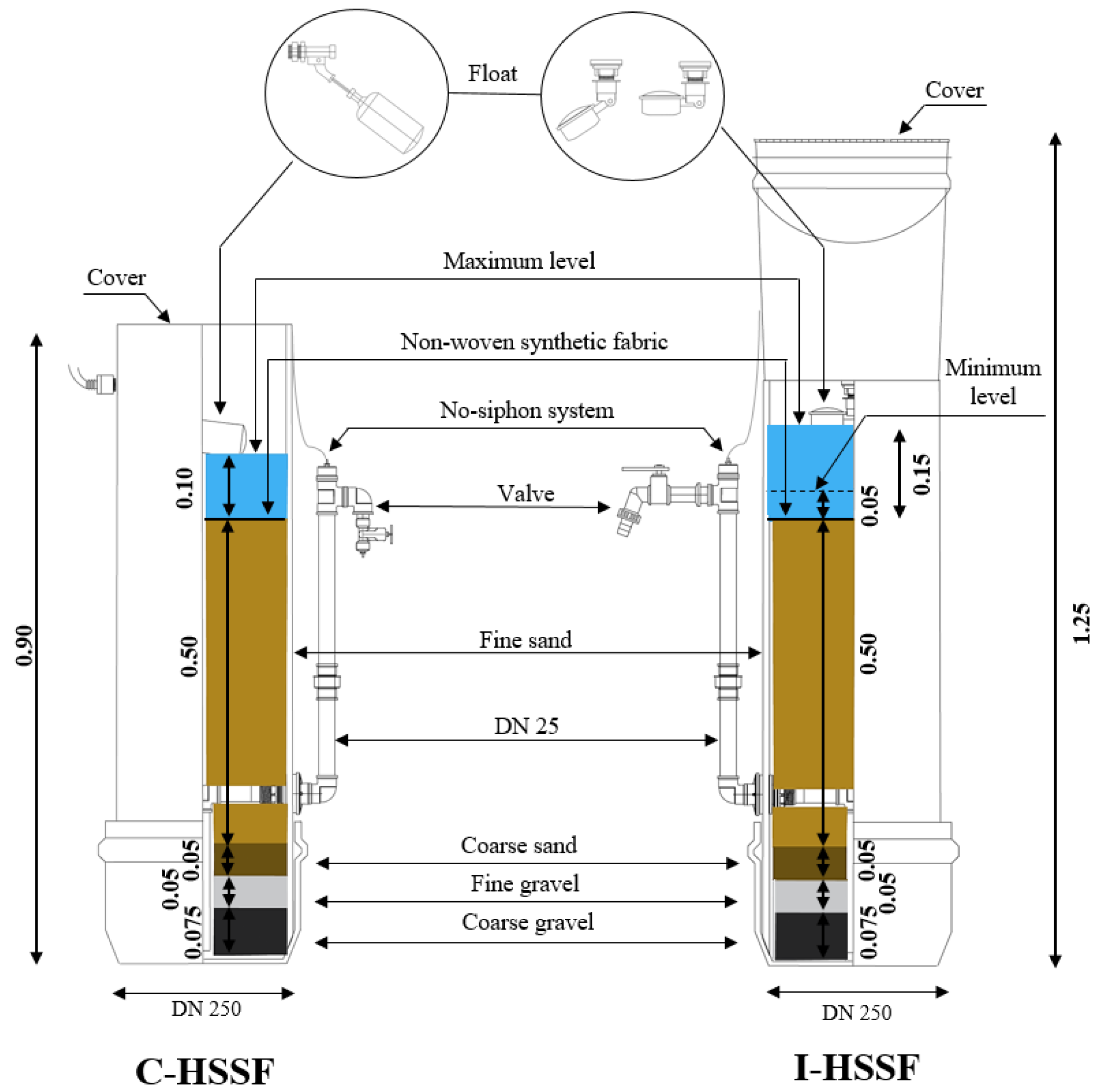
2.1. Household Slow Sand Filters

Two HSSFs were studied; one was operated in continuous flow (C-HSSF) and the other one in intermittent flow (I-HSSF). Both were made of PVC DEFoFo pipe (diameter 250 mm, area 0.053 m²). The filtration layer was 50 cm of fine sand (0.17–0.56 mm; effective size 0.17 mm; uniformity coefficient 2.27; porosity 37%), a 5 cm support layer of coarse sand (0.17–0.67 mm), 5 cm layer of fine gravel (5.0–7.0 mm) and 7.5 cm layer of coarse gravel (7.0–12.0 mm). All materials were bought locally (São Carlos, Brazil), washed, sun-dried and sieved. A non-woven synthetic fabric (specific gravity 0.2 g cm⁻³; 100% polyester; thickness 2 mm) was placed at the sand layer top ease maintenance (Figure 1).

2.2. Filters Preparation and Experimental Set-Up

Water used was collected from the Monjolinho River (São Carlos Brazil). The filters were fed with raw water that was previously settled (24 h) followed by filtration through two layers of felt blanket. Pre-treated water quality had turbidity (6.9 ± 3.4) NTU, apparent color (36.1 ± 13.5) HU, TC (4649 ± 6526) CFU 100 mL⁻¹, E. coli (366 ± 109) CFU 100 mL⁻¹. Pre-treated water was pumped into an elevated tank, coming through a side perforation above the filter top. In the C-HSSF, the filtration rate was constant (0.90 m³ m⁻² day⁻¹) throughout the experiment. For the I-HSSF, 16 L pre-treated water fed the filter three times per day (8:00 a.m., 1:00, and 6:00 p.m.). The filtration rate reached its maximum (3.21 ± 1.18 m³ m⁻² day⁻¹) when fed, and it gradually decreased to zero. The daily production of both HSSFs was 48 L, which could provide the minimum acceptable for domestic use for six people (7.5 L hab⁻¹ d⁻¹) [30].

2.3. Filters Removal Efficiencies

One Litre samples of pre-treated and filtered water were collected and measured daily from day zero, for seven weeks. Each sample was homogenized and 100 mL was used for quantification of E. coli and TC by membrane filtration (0.45 µm) and plate counting using Chromocult^® Coliform Agar (Merck, Darmstadt, Germany). Turbidity and apparent color were measured using a turbidimeter (Hach 2100N, Ames, IA, USA) and a colorimeter (DM-COR Digimed, São Paulo, Brazil).

The datasets were tested to determine if they were normally or non-normally distributed, using the Shapiro–Wilk test. When normally distributed, paired or non-paired, a T-test was used to compare if there was a significant difference between water samples. The equivalent non-parametric tests of Wilcoxon (paired) and Mann–Whitney (non-paired) were used when the datasets were non-normally distributed. Pearson correlation test (parametric) or Spearman correlation test (non-parametric) were used to determine the correlation between two datasets. All statistical tests were performed considering a 95% confidence interval.

The correlation between the EPS concentrations and the HHSF efficiency was measured by Pearson’s correlation coefficients (r). They were calculated using the weekly average data of all the daily values of the following parameters, total carbohydrates and total proteins from the blanket and the sand samples, reduction of E. coli, TC, turbidity, and color after filtration with both, C-HSSF and I-HSSF. The significance levels are the following: *** for r ≥ 0.898, p < 0.001, ** for r ≥ 0.797, p < 0.01, and * for r ≥ 0.582, p < 0.01.

2.4. Biofilm Characterization

2.4.1. Sampling and EPS Analysis

For each HSSF, six sand core samples were extracted at 5 mm depth using a cut-off syringe (10 mm diameter). Each core contained approximately 0.5 g (±0.1) of sand, individually weighed after extraction. Felt blanket samples were also taken with a cut-off syringe from the blanket’s surface. 0.5 mL of liquid samples were frozen at −20 °C until further analysis. Sampling took place once per week. EPS content from the sand cores was extracted as follows [31]. The sand samples were placed in 2 mL tubes and mixed with distilled water at 20 °C for 1.5 h (Mixer, Spiramix 5, Denley Inst., Heckmondwike, UK). After sedimentation for 1.0 h at 20 °C, the supernatant containing the colloidal EPS fraction was extracted. Then, the supernatant was analyzed for carbohydrates and proteins following the phenol assay protocol [32] and the modified Lowry procedure [33]. Briefly, for carbohydrates, 200 µL phenol (5%) and 1 mL sulphuric acid (98%) were added to 200 µL of supernatant and then incubated 35 min at 30 °C. For proteins, 250 μL supernatant were incubated 15 min with 250 μL of 2% sodium dodecyl sulfate salt and 700 μL of ‘chemical reagent 4’ and incubated for 45 min at 30 °C with Folin reagent [34].

The carbohydrate concentration was measured with a spectrophotometer (CECIL CE3021, Cambridge, UK) at 488 nm and proteins at 750 nm. Calibration curves (0–200 mg mL⁻¹) of carbohydrates and proteins were made with D-glucose and bovine serum albumin (Sigma-Aldrich, San Luis, CA, USA), respectively [32,34].

For sand samples, after extraction, the tubes containing the remaining sand were dried in a cabinet (Gehaka G4023D, São Paulo, Brazil) at 80 °C for 2 h. Then the dehydrated sand was weighed to determine the mass of polysaccharides and proteins per mass of dry sand (mg g⁻¹). For the blanket samples, the carbohydrate and protein concentrations are given in terms of the mass of either protein or polysaccharides per volume of liquid sample (mg mL⁻¹).

2.4.2. Microbial Community

To identify the microorganisms present in the schmutzdecke, aliquots of the sediment on the top of the felt blanket and fractions of sand were analyzed. For samples collection, first, the felt blanket was removed from the filter and placed in a tray. The accumulated sediment on the blanket was gently scraped with a spatula, including the corners, and the content was transferred to 50 mL tubes. For the biofilm formed on the sand top, a 5 cm layer of the sand filter was collected in a tray, washed three times with 100 mL distilled water each, and transferred to 50 mL plastic centrifuge tubes. The sand tubes were centrifuged (1500× g, 15 min), then the supernatant was discarded, and the tube was filled again with distilled water. This process was repeated three times. For the visualization and identification of organisms, one drop of the pellet was placed in a glass slide, covered with a coverslip and observed in an optic microscopic (BX51, Olympus^®, Tokyo, Japan) in the bright field under the 40× objective.

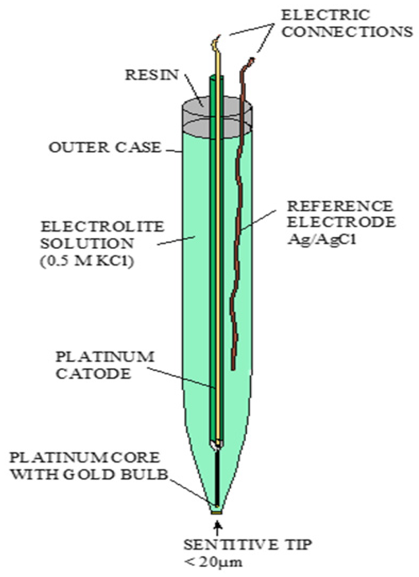
2.5. Dissolved Oxygen (DO)

The DO microsensors used were constructed from platinum and silver wires as described elsewhere [35,36]. 50 µm diameter platinum wires bathed in an etching solution were used for the cathodes. At the cathode end, a gold solution (HAuCl₄·3H₂O) was electrolyzed to form a bulb with appropriate conductive characteristics. To make the anodes, 300 µm diameter silver wires were used (Ag/AgCl reference electrodes). The outer compartment of the microsensors was constructed from glass Pasteur pipettes, which had their tips properly moulded. The compartments received the gas selective membrane produced with silicone glue (Figure A1). The calibration was made with saturated O₂ water (7.8 mg L⁻¹) and sodium sulphite solution 5% (zero). Microsensors were introduced vertically into the non-woven blanket samples with the aid of a controlled micro stepper with a spatial resolution of 20 µm. DO measurements were taken vertically with the supports immersed in water from the filters as described elsewhere [36]. For each measuring point, DO analyses at the beginning and the end of the filtration run were made.

2.6. Biomass Content

The biomass developed on the felt blanket and the first centimeters of sand were determined by volatile suspended solids (VSS). For sample collection, the filter faucet was closed, then the blanket was removed, scraped, and washed with deionized water until complete cleaning; after this, the water on the sand layer top was removed and discarded; then the top of the sand layer (few cm) was scraped, transferred to a bottle and stirred with deionized water until complete cleaning; and finally the residue from the felt blanket and sand washing were handled as samples. The biomass content was determined in triplicate before (day 0) and at the end of the experiment (day 48).

2.7. Temperature

The temperature inside the filters and the ambient temperature were measured daily, at the same time using digital thermometers (Dugold, Conde, Brazil). For HSSFs, the external sensors were positioned in the stead water above the sand, while for ambient temperature, the sensor was located near the elevated pre-treated water tank.

3. Results

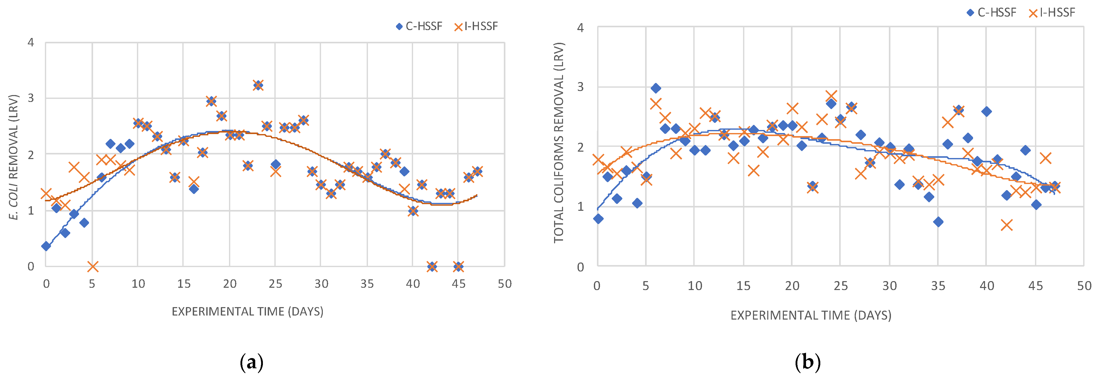
3.1. Removal of E. coli and TC in C-HSSF and I-HSSF

The E. coli and TC reduction were determined every day for 48 days (Figure 2). TC in filtered water samples were 76 ± 234 CFU 100 mL⁻¹ for C-HSSF and 42 ± 41 CFU 100 mL⁻¹ for I-HSSF. TC removal of the whole period was 1.88 ± 0.54 log for C-HSSF and 1.91 ± 0.48 log for I-HSSF, with a maximum TC reduction of 2.98-log and 2.85-log by the C-HSSF and I-HSSF, respectively. E. coli concentrations in filtered water were 20 ± 111 CFU 100 mL⁻¹ for C-HSSF and 4 ± 15 CFU 100 mL⁻¹ for I-HSSF. Due to external factors, e.g., real water demands, water pollution in real conditions, etc., important fluctuations were registered in the E. coli and TC concentrations at the influent and, therefore, in their removals (Figure 2). Removal rates were 1.71 ± 0.79 logs and 1.77 ± 0.68 logs for C-HSSF and I-HSSF, respectively, with a maximum reduction of 3.23 log for both filters. The absence of E. coli in 100 mL was observed in 58.3% of the samples from C-HSSF and 47.9% from I-HSSF. There was no significant difference between the efficiencies of HSSF models for TC (paired T-test, p = 0.27) and E. coli removal (Wilcoxon test, p = 0.21).

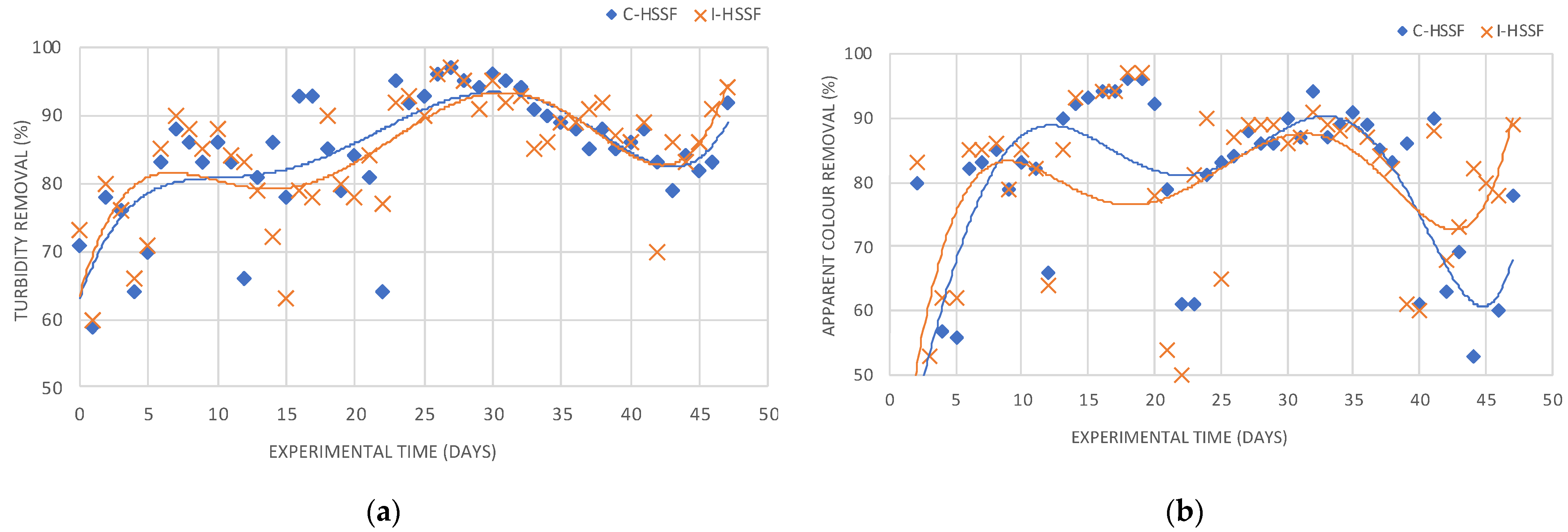
3.2. Turbidity and Apparent Color Removal in C-HSSF and I-HSSF

Both filters presented a similar turbidity removal (Figure 3a). C-HSSF removed 85% ± 9% and I-HSSF 84% ± 9%, leading to final turbidity of 0.91 ± 0.49 NTU and 0.93 ± 0.46 NTU, respectively. It was also observed a correlation between removal rate and the period of operation (Spearman’s correlation; C-HSSF: r_s = 0.426, p = 0.002; I-HSSF: r_s = 0.499, p < 0.001). Regarding apparent color reduction, both filters reached 77% (Figure 3b) yielding water with a residual average apparent color of 8.61 ± 7.96 HU and 8.03 ± 6.94 HU, respectively. There was no correlation between residual apparent color, apparent color removal, influent apparent color, and day of operation, for either of the filters.

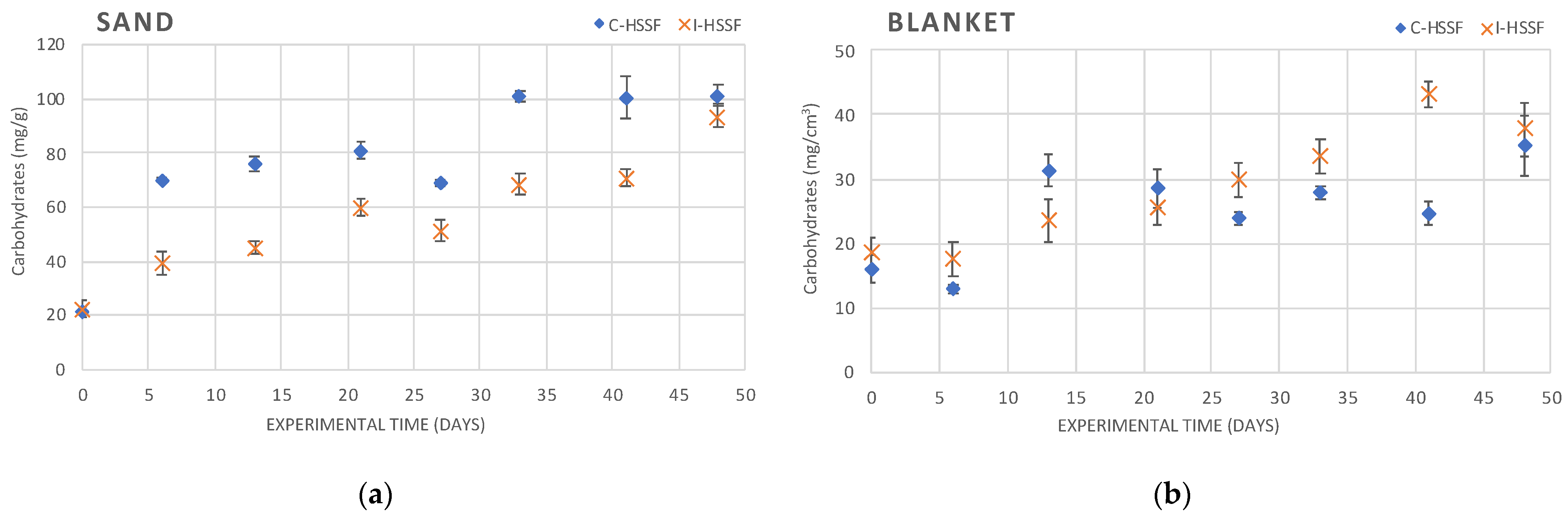
3.3. Determination of EPS in C-HSSF and I-HSSF

3.3.1. Carbohydrates in the Sand and Blanket of C-HSSF and I-HSSF

The colloidal carbohydrate concentrations increased over time in both HSSFs (Figure 4a). The increase was most pronounced for the C-HSSF, up to 4.7 times compared to 3 times in the I-HSSF. In week 4, a significant drop (up to 14%), however, non-statistical difference between week 3 and 4 was observed in both C-HSSF (p = 0.61) and I-HSSF (p = 0.39). The carbohydrate concentration varied between 21.4 and 101.2 mg g⁻¹ for C-HSSF and from 22.5 to 93.9 mg g⁻¹ (p = 0.79) for I-HSSF with significantly different means in the treatments for all sampling dates (p = 0.006) except the first and last day of the experiment (Figure 4a). The carbohydrates concentrations were higher in the C-HSSF compared to the I-HSSF (week 1 p < 0.007). For the C-HSSF, the colloidal carbohydrate concentration increased until week 5 (101.2 mg g⁻¹), then no significant differences were found between weeks 5, 6, and 7 (p = 0.96–0.99). For I-HSSF, carbohydrates concentration was not significantly different between weeks 5 and 6 (p = 0.87), however, in week 7, the concentration increased up to 25% and finally was not significantly different to the C-HSSF (p = 0.31).

In the C-HSSF filter, the total colloidal carbohydrates concentrations extracted from the blanket varied between 16 and 35 mg mL⁻¹, while for the I-HSSF they varied between 18 and 43 mg mL⁻¹ (Figure 4b). For both C-HSSF and I-HSSF, the carbohydrates concentrations were not significantly different in the first week of the experiment (week 0: p = 0.38; week 1: p = 0.17). In week 2 a significant increase was observed in both filters up to 95% (p = 0.02) and up to 27% (p = 0.03) for the C-HSSF and I-HSSF, respectively. Then, the carbohydrate concentration slightly decreased thereafter in C-HSSF with no significantly different means in weeks 4–7 (p = 1, p = 0.90, p = 0.11). In contrast, in the I-HSSF, the carbohydrates concentration showed a continuing increase up to week 6 which stabilised in week 7 at around 40%. The weekly average values of carbohydrate concentrations for C-HSSF and I-HSSF were not significantly different (p = 0.46).

3.3.2. Proteins in the Sand and Blanket of C-HSSF and I-HSSF

The water-extractable proteins showed a clear increase up to 8.8 times over the first two weeks of the experiment for C-HSSF and a decrease thereafter up to 72% (Figure 5a). The protein concentrations for the treatment of C-HSSF varied between 34.9 and 307.8 mg g⁻¹. Protein concentration in I-HSSF was negligible at the beginning of the experiment, then it showed a continuous increase up to 217 mg g⁻¹ until week 5, and then slightly decreased thereafter. With no significantly different means in the treatment for most of the sampling dates (p = 0.56). The patterns of the protein concentrations in the blanket of C-HSSF and I-HSSF were similar, with an increase towards week 3 and a gradual decrease thereafter (Figure 5b). The protein concentration varied between 32.3 and 73.5 mg mL⁻¹ for C-HSSF and from 37.5 and 74.6 mg mL⁻¹ for I-HSSF, respectively, with no significantly different means (p = 0.78) in the treatments for all sampling dates.

3.4. Microscopic Analysis

The microorganisms from biofilm (blanket and sand) from C-HSSF and I-HSFF, identified by bright field microscopy, are listed in

Table 1. Microorganisms identified by bright field microscopy in samples collected from blanket and sand from C-HSSF and I-HSSF.

Class	Microorganism	C-HSSF		I-HSSF
		Blanket	Sand	Blanket	Sand
	Chilomonas spp.			X
	Chlorella spp.			X	X
	Clamydomonas spp.	X	X		X
	Coelastrum spp.	X	X
	Cryptomonas spp.				X
	Desmodesmus spp.	X	X
	Eudoria spp.
	Euglena spp.			X	X
Algae	Meliosira spp.			X
	Navicula spp.			X
	Nitzchia spp.		X
	Phacus spp.			X
	Phytoconis spp.				X
	Rhodomonas spp.	X	X	X
	Scenedesmus spp.	X	X	X	X
	Staurodesmus spp.	X	X
	Trachelomonas spp.	X	X
Helmints	Nematode (filarial larvae)		X
	Aspidisca spp.		X	X	X
	Entamoeba spp.	X	X	X	X
Protozoa	Giardia spp.	X	X		X
	Heliozoa	X		X
	Vorticela spp.	X		X

X indicates the presence of microorganisms, and empty space indicates the absence of microorganisms.

. In both filters, the microbiological composition of the schmutzdecke were essentially the same.

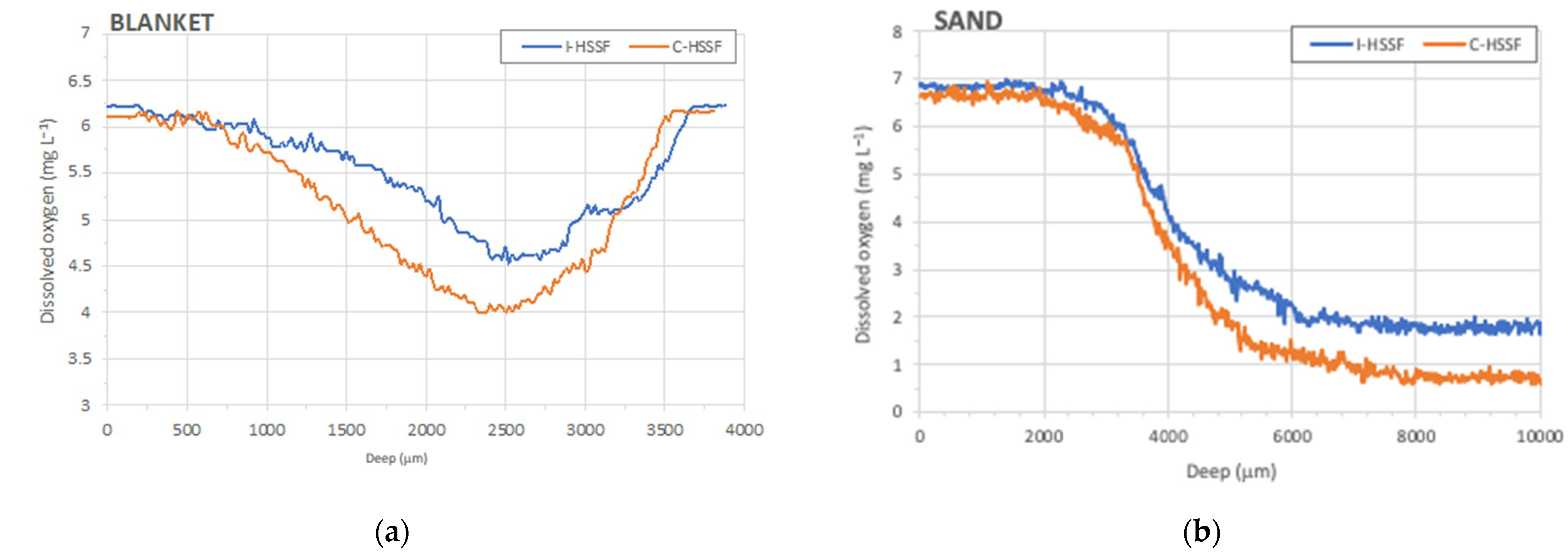
3.5. Dissolved Oxygen

In the beginning, the DO concentrations correspond to the influent water, being 6.21 and 6.11 mg L⁻¹ for I-HSSF and C-HSSF. After 48 days, the minimum DO of 4.57 mg L⁻¹ for I-HSSF and 4.0 mg L⁻¹ for C-HSSF were registered in the blanket. The maximum DO depletion induced by the biofilms adhered to the blankets was observed as 1.64 mg L⁻¹ for I-HSSF and 2.11 mg L⁻¹ for C-HSSF (Figure 6a). The initial DO concentrations (≅6.8 mg L⁻¹) decreased after 2 mm when the sensitive tip of the microsensors touched the sandy surface. At approximately 4 mm depth of the sandy bed, the DO concentration for I-HSSF remained around 1.70 mg L⁻¹ and 0.64 mg L⁻¹ for C-HSSF. The maximum depletion of DO observed—calculated as DO_final–DO_initial—in the sand for I-HSSF was 5.15 mg L⁻¹ and for C-HSSF was 6.00 mg L⁻¹ (Figure 6b).

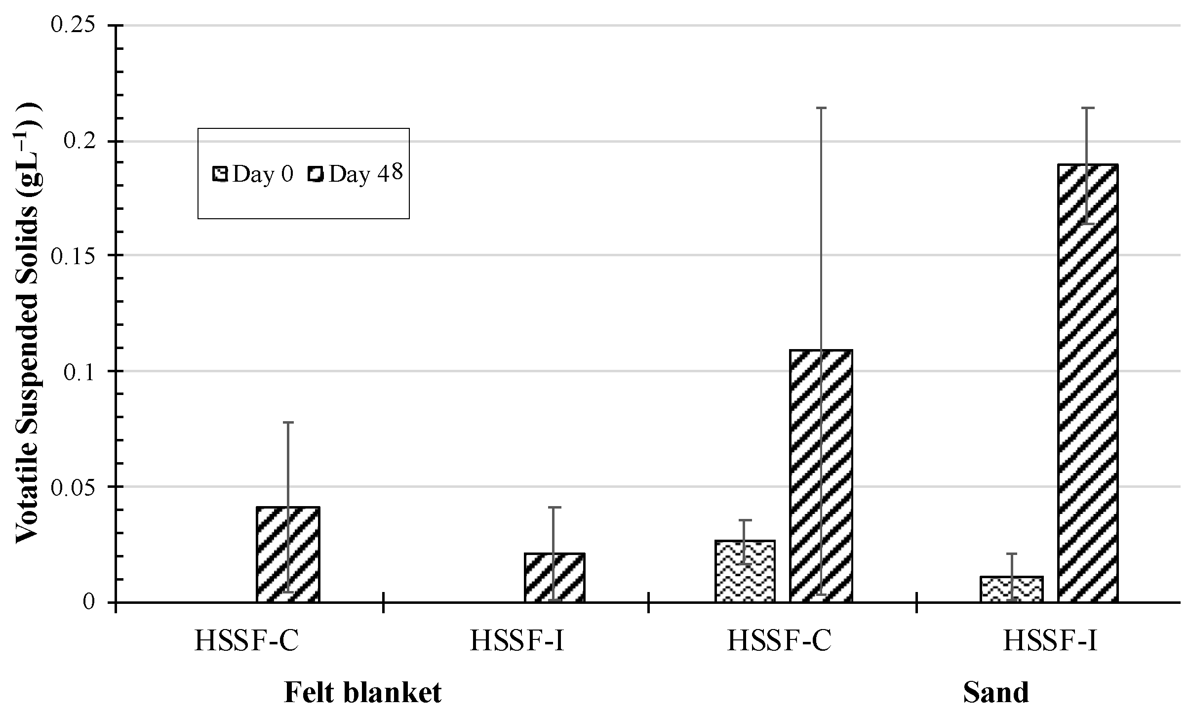
3.6. Biomass Content

The biomass content in the blanket and sand of C-HSSF and I-HSSF was measured by VSS (Figure 7). The sand samples showed little values of biomass at the beginning of the filter operation (<0.03 mg L⁻¹), while no volatile solids were observed in blanket samples at day zero. All samples showed an increase in biomass when comparing the beginning (day 0) and the end of the operation (day 48), from 0.03 to 0.11 g L⁻¹ for the C-HSSF and from <0.03 to 0.19 g L⁻¹ in the I-HSSF. C-HSSF presented greater biomass accumulation in the blanket (0.04 mg L⁻¹) than I-HSSF (0.03 mg L⁻¹). On the other hand, greater concentrations of volatile solids were observed in the sand samples from I-HSSF, than C-HSSF.

3.7. Analysis and Modelling of HSSFs Performance against EPS

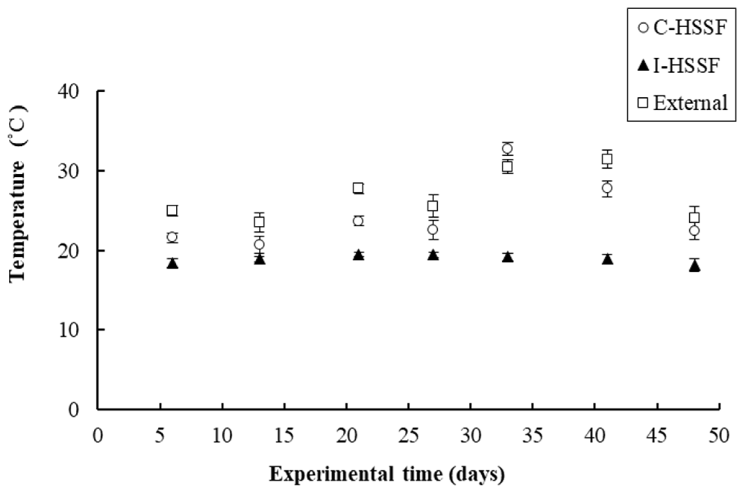
Pearson’s correlation coefficients (r) between EPS carbohydrates and EPS protein extracted from the blanket and sand and the reduction of E. coli and TC (

Table 2. Pearson’s correlation coefficients (r) between EPS carbohydrates and EPS protein extracted from the blanket and sand in the C-HSSF and I-HSSF as well as reduction of E. coli, TC (LRV), turbidity (%), and color (%).

C-HSSF
Reduction of #	Carbohydrates			Protein
	Blanket	Sand	Blanket	Sand
E. coli	0.434	0.135	0.883 **	0.194
TC	0.379	0.265	0.893 ***	0.139
Turbidity	0.595 *	0.616 *	0.529	0.069
Color	0.546	0.355	0.798 **	0.141
I-HSSF
Reduction of #	Carbohydrates		Protein
	Blanket	Sand	Blanket	Sand
E. coli	0.131	0.399	0.896 ***	0.665 *
TC	0.371	0.164	0.709 **	0.322
Turbidity	0.687 *	0.550	0.243	0.637 *
Color	0.561	0.437	0.354	0.767 *

The significance levels are, *** p < 0.001, ** p < 0.01, * p < 0.1. Values of r above 0.7 are bold highlighted.

), turbidity, and color in C-HSSF and I-HSSF was calculated. Different grades of correlation can be observed: none or weak (r < 0.582), moderate (0.582 < r < 0.797), and high (r > 0.797). For C-HSSF, there was a moderate correlation between carbohydrates in the blanket and from the sand, while the proteins from the blanket were strongly linked to the removal of E. coli, TC and color. No significant correlations were found between proteins from sand and the analyzed parameters. For I-HSSF, the EPS carbohydrates in the blanket were moderately correlated with turbidity reduction (r = 0.687, p < 0.1) but not as much with the carbohydrates extracted from the sand (r = 0.550). For proteins in the blanket, there was again a strong correlation with the E. coli, TC, and color reduction, with a moderate link between proteins from the sand and the reduction of E. coli, turbidity, and color removal.

3.8. Temperature

Ambient temperature (Figure A2) was highly significantly correlated with temperature in the C-HSSF (Pearson’s correlation, r = 0.958, p < 0.001) and I-HSSF (r = 0.949, p < 0.001). The temperature in I-HSSF was 6.7 °C lower than the external temperature and 3.5 °C less than inside C-HSSF. Due to heavy rain in week four, a drop of 2 °C was observed in ambient and both filters’ temperatures. The maximum temperature was recorded in week 5, with 32.7 °C ambient and 29.2 °C and 25.3 °C in the C-HSSF and I-HSSF, respectively.

4. Discussion

HSSF is a simple and energy-efficient water treatment technology of potable drinking water. Most published studies focused on engineering characterization, i.e., operation and optimization for better efficiency. However, there is a gap concerning schmutzdecke physicochemical and structural properties and their relationship with the efficiency of water quality indicators [37].

The results pointed out in items 3.1 and 3.2 reiterates the capability of HSSF in removing particles organics and inorganics, including pathogens from the water, hence improving its quality [10,16,37,38].

The removal rates for E. coli and TC were within the range reported by several authors, for both HSSFs, varying from 0.3 to 4.0 log for E. coli and from 0.4 to 3.6 log for total coliforms [6,8,9,13,39,40], even though it was not enough for the treated water to reach the potability standards established by the WHO [41], i.e., absence of microorganisms, requiring a post-treatment.

The variations observed in the E. coli and coliform removal graphics, translated into the high or low peaks, were related to the influent water. Due to external factors, the concentration of bacteria in the water to be treated was very high or very low on some days, which generated great variations in the system, without necessarily being related to the increase or decrease in the efficiency of the filters. The same did not happen with turbidity, whose daily values in the raw water remained similar throughout the study.

Turbidity reductions observed were following the literature, from 78.4 to 96% for I-HSSF [9,40] and from 89.4 to 96.8% for C-HSSF [8,42]. Furthermore, both filters achieved turbidity values below 5 NTU, meeting the maximum level established by WHO. Regarding color removal, there are only recommendations for acceptable drinking water. A color below 15 HU might reduce the user’s rejection of being undetectable in a glass of water [41]. Therefore, with apparent color below 10 HU, filtered water from both filters presented a low rejected risk. Color removal rates of almost 80% were expected for both filters [2].

In this study, turbidity removal correlated with operation time, improving over the days as observed elsewhere [6,8,9]. This can be attributed to the schmutzdecke development and the ripening of the filter bed, as well as the reduction in filtration rate and the increase in water exposure to treatment mechanisms [38]. On the other hand, no correlation between operation time and bacteria removal (E. coli and total coliforms) has been observed in our study.

The efficiency of SSF with biological layer to retain of E. coli ~96% compared to sand filter ~35% were reported [43] and explained by higher pathogen adsorption rate on the biological layer (schmutzdecke), hence absorption of fecal indicator bacteria (FIB) on the filter bed can be expected as a minor contribution of the overall removal.

Our results suggest the predominance of proteins over carbohydrates up to 3 times in the C-HSSF and 2.3 times in the I-HSSF sand samples, and up to 2 times in the blanket. That can be attributed to dominant bacteria over algae in the biofilm, as generally bacteria are mainly associated with protein secretion [18], while algae produce a greater proportion of polysaccharides [44]. Nevertheless, carbohydrates and proteins are not exclusively linked to microalgae or bacteria [31], and their proportion might vary between and within species.

To our knowledge, the relationship between carbohydrates and proteins accumulated in HSSFs and their water treatment efficiency has been rarely investigated. Unger and Collins reported the absence of correlation between EPS compounds total carbohydrate and total proteins and bacterial removal and claim that the development of a schmuzdecke does not improve E. coli removal [30]. In contrast, in the present study, highly significant correlations have been found between concentrations of proteins and reduction of E. coli, TC, and color in C-HSSF and I-HSSF, while the correlation with carbohydrates is only moderate (Table 2). After one week, the efficiency of filters to retain microorganisms raised to 2 times (C-HSSF) and 1.6 times (I-HSSF) compared to their initial capacity. This increase was even more marked in week four (Figure 2 and Figure 3) and it is linked to the development of biofilms inside the filters, as also demonstrated by the correlation factors (Table 2) of EPS concentrations and removal efficiency for bacteria and color. However, this correlation is not linear. For example, the I-HSSF efficiency increased up to 6.3 times by the end of the experiment compared to the first day, while protein concentration in the blanket increased by 2.3 times (Table 2). The role of carbohydrates is still unclear. Some authors point out that they could interact with proteins to form a resilient matrix similar to epoxy resin [45] and induce a synergistic effect between carbohydrates and proteins. What seems clear is that the quantified EPS presence can be used to understand the mechanism of maturation of the biofilms in HSSF, although the EPS-quantity per se cannot be used as a predictor of the filter’s efficiency.

In the present study, inside of both filters C-HSSF and I-HSSF, the blanket has been used to facilitate the maintenance (cleaning) of the filters. The blanket acts as a porous filter medium in open filters, preventing the fast clogging of the sand bed and may provide better support for initial microbial attachment than sand particles. Thus, in this study, we quantitatively analyzed and compared EPS components extracted from the top of the sand of the schmutzdecke layer and samples collected from the blanket of HSSFs.

Assuming the density of fine sand is 1.45 mg cm⁻³, the ratio of total carbohydrates in the top of the sand was 5 times greater than in the blanket in C-HSSF and 3 times greater in I-HSSF, while the total protein was 5.5- and 4.3-times greater in the top of the sand samples and blanket for C-HSSF and I-HSSF, respectively. These results suggest stronger biofilm development at the top of the sand than in the blanket. Therefore, our results also suggest that the schmutzdecke layer has a more important effect than the blanket in the efficiency of the HSSFs, as also suggested by Ranjan and Prem [15].

The diversity of organisms (algae, helminth, protozoa) revealed by the microscopic analyses (Table 1) demonstrates the existence of an established and mature schmutzdecke inside the filters, as reported before [8,9,25,46]. This result added to the balanced distribution of the types of microorganisms between the two filters indicates that the mode of operation did not influence the entry of the microorganisms present in the raw water, in the filters, and most likely should not interfere in the structuring, formation, and maintenance of biofilms.

Among the microorganisms found (algae, helminth, and protozoa), algae stood out as the most prevalent, in both filters, with 17 different genera observed in the analyzed samples. This fact can be attributed to the characteristic of the influent water, which is directly responsible for the chemical and biological composition of the biofilm [25]. In this case, particularly, the water came from the river and, therefore, remained exposed to sunlight, which favors the algae reproduction [47].

The analyses also highlighted a greater number of organisms in the biofilm formed in the blanket compared to the top of the sand in both filters. This can be explained by the position of the blanket within the filter, which makes it the first water contact surface and the first physical barrier promoting partial retention of organic matter, including microorganisms [8,46,48] and consequently stimulating the development of a robust biological layer.

The importance of microorganisms in SSFs is widely appreciated [49]. As mentioned, algae produce carbohydrates which are primarily responsible for giving elasticity and viscosity, making the biological layer more resistant and more adherent [44]. Some microalgae species also suppress bacteria levels by producing polyunsaturated aldehydes [50] or antibacterial toxins, inducing strong bactericidal effects [27]. The presence of protozoa in schmutzdecke also has beneficial implications for water quality. Initially, it indicates that the biological layer is active, retaining these and other organisms, removing them from the water. Some protozoa can improve bacteria removal by the interception and predation of bacteria in the bulk fluid flow and the grazing surface-associated bacteria [29]. They can also be responsible for the removal of other types of suspended solids, liberating flow pores for water permeation and new microbial colonization, optimizing the filtration process [49]. In addition, some protozoans such as Aspidisca spp. and Vorticella spp., both found in this study, can ingest cysts and oocysts, contributing to their reduction in the filtered water [51].

The biomass results are also evidence of biological layer development in the sand and the blanket [8,9,40]. However, the biomass amount was more abundant at the sand top than at the blanket, regardless of operation regimes (T-test, p = 0.007). During the 48 days of operation, I-HSSF presented a more pronounced biomass increase in the sand top, while, for C-HSSF the biomass increase was observed in the blanket. These results can be explained by a higher filtration rate and water level of the I-HSSF, which increases the water flow into the sand, reducing blanket retaining. The biomass developed in the filters after 48 days of operation was another evidence of the biological layer development, which can also explain the decreased microbial load and the input of particles from influent water, as shown in Section 3.1 and 3.2.

DO profiles for sand samples show a depletion due to the respiration of microorganisms in their metabolic activities and to the chemical action of particulate material deposited on the blanket and sand [15,36]. This DO profile reflects the progressive growth of biofilms in the upper layer of the HSSF, which can explain the gradual improvement in the removal efficiency of E. coli, TC, turbidity, and apparent color [36]. Although both indicate biofilm activity, DO profiles of blanket and sand present different trends due to the sample type. At the beginning and end of the blanket profile, DO values were almost the same. It occurred because the microsensors crossed the entire blanket thickness and made contact again with the immersion water below the blankets. Comparing these profiles, the minimum DO concentration on the blankets is higher than those of sand beds. This can be attributed to the position of the blanket within the filter, which is the first contact surface receiving the influent water (with higher DO) and microorganisms.

Regarding the two flow regimes, DO profiles of both C-HSSF and I-HSSF showed similar trends but also a higher DO depletion in the C-HSSF than in I-HSSF. Considering that both had the same influent water, this difference can be attributed to the continuous supply of the filter, which may affect the adherence of the schmutzdecke as well as its maturation process [52]. This includes not only the sedimentation of suspended particulate matter but also the mass transfer on a microscale [36,52].

The temperature has a strong effect on the performance of HSSF. Unger and Collins [30] showed that warm (24 °C) biological columns outperformed colder (8 °C) biological columns in E. coli removal. It is generally recommended, for satisfactory biochemical oxidation of organic matter, to avoid temperature falling too low [15]. Due to heavy rain in week 4, the external temperature dropped 2 °C, and consequently, the temperature also dropped in both filters up to 18.6 °C (C-HSSF) and 15.5 °C (I-HSSF). Despite the absence of correlation between temperature and EPS production, this drop was mirrored by the drop in EPS carbohydrates and EPS protein in sand samples in week 4. However, these temperature variations did not affect the efficiency of both filters. Probably the spatial variation within 5 °C does not affect the performance of HSSF. This finding was confirmed by the results of the performance of both filters: despite that temperature of I-HSSF was on average 3.5 °C less than the temperature in C-HSSF, both models show similar performance in organic and inorganic removals. It also could be due to the biofilm being matured enough up to week 4 and achieving a steady-state phase; then, temperature variation does not significantly affect the performance of the filters in this stage.

Comparing both C-HSSF and I-HSSF, our results show that there was no significant difference in the efficiencies for the removal of bacteria, turbidity, and apparent color, indicating that the flow regime did not influence the performance. Similarly, C-HSSF and I-HSSF EPS results also showed similar behavior; a highly significant correlation between protein concentration in the blanket with bacterial removal, a moderate correlation between carbohydrates in blanket and sand, and turbidity removal (Table 2). This suggests a clear similarity of the biofilm development in both filters. Regardless of the differences inherent in the distinct operation, there were no overall statistical differences between the data from the models (p ≥ 0.05). Our findings indicate that the operation regime did not significantly affect schmutzdecke development and, consequently, filter efficiency. These results were consistent with the relationship between HSSF microbiological development and its efficiency (Elliott et al., 2008) and differ from the previously reported comparison between bench-scale [4] and household-scale [6,53] continuous and intermittent filters.

The schmutzdecke of a household slow sand filter is a highly complex and dynamic environment, which is under constant adaptation and transformation. The literature indicates that the schmutzdecke takes, on average, 30 days of operation to become mature [2,21] but also highlights that this number can vary depending on several external factors [15]. Therefore, our study was performed for a longer period of time than that described in the literature (30 days). However, even so, the filters did not reach their full reduction capacity and would likely have continued to improve beyond this period. Therefore, further experimentation is recommended to shed light on this possibility.

Further studies that identify the separate contribution of both filtration mechanisms, physical and biological, in HSSF might be of interest to determine the role of the schutmuzdecke. This could be carried out by comparing results of replicated tests where one has its normal functioning and the other with the chemical inhibition of schutmuzdecke (e.g., sodium azide). While the former would provide a complete scenario of the two combined mechanisms, the latter would have only physical activity to improve water quality. In a recent review paper, Freitas et al. (2022) pointed out the schtmuzdecke impact on the HSSF efficiency [38], however, they highlighted that individual and synergistic contributions of physical and biological characteristics still need further research.

5. Conclusions

The ability of HSSF in improving water quality was evidenced by the results presented herein, although there was no complete removal of bacteria (E. coli and TC), requiring a post-treatment for complete water disinfection.

One of the many advantages of HSSFs over other domestic water technologies is the formation of the biological layer at the top of the filter bed that acts as an additional water treatment increasing the efficiency of the system. Compiling the information generated by the techniques applied in this study, including taxonomy, DO monitoring, biomass and EPS determinations, it was possible to observe the gradual formation and ripening mature schmutzdecke that helped to maintain a degree of bacterial removal, color, and turbidity reduction over 7 weeks. The EPS analyses also indicate the predominance of proteins over carbohydrates up to 3 times in both HSSF in sand and blanket.

The efficiency of filters to retain bacteria (E. coli and TC) and remove color was highly significantly correlated with EPS protein concentration and turbidity reduction significantly correlated with EPS carbohydrates. However, the EPS quantity per se cannot be used as a predictor of the filter’s efficiency.

The schmutzdecke formed on the top of the blanket and the sand developed differently. However, the water supply regime did not seem to influence its overall development efficiency since no significant differences were observed between filters.

The results presented in this work had better helped further elucidate the relationship between the biological layer and the water purification process by HSSF. However, there are still some unknowns regarding the influence of the variables analyzed herein, on the matrix formation and growth in filtration systems, especially the ripening time. Longer filtration runs can mean greater system efficiency. Therefore, interdisciplinary approaches are strongly recommended to enhance the knowledge about schmutzdecke contributions to drinking water conditioning processes in waterworks.

References

1. WHO. Progress on Drinking Water and Sanitation; World Health Organization: Geneva, Switzerland, 2012. [Google Scholar]
2. Centre for Affordable and Water Sanitation and Technology (CAWST). Biosand Filter Construction Manual; Centre for Affordable Water and Sanitation Technology: Calgary, AB, Canada, 2012. [Google Scholar]
3. Sheikh, M.A.; Mustufa, M.A.; Laghari, T.M.; Manzoor, B.; Haider, S.A.; Bibi, S.; Ali, F.I. Prevalence of Waterborne Diseases in Exposed and Unexposed Clusters Using Biosand Filters in a Rural Community, Sindh, Pakistan. Expos. Health 2016, 8, 193–198. [Google Scholar] [CrossRef]
4. Young-Rojanschi, C.; Madramootoo, C. Intermittent Versus Continuous Operation of Biosand Filters. Water Res. 2014, 45, 1–10. [Google Scholar] [CrossRef]
5. Andreoli, F.C.; Sabogal-Paz, L.P. Household slow sand filter to treat groundwater with microbiological risks in rural communities. Water Res. 2020, 186, 116352. [Google Scholar] [CrossRef] [PubMed]
6. Faria Maciel, P.M.; Sabogal-Paz, L.P. Household slow sand filters with and without water level control: Continuous and intermittent flow. Environ. Technol. 2018, 41, 944–958. [Google Scholar] [CrossRef] [PubMed]
7. Schijvena, J.F.; van den Bergg, H.H.J.L.; Colin, M.; Dullemont, Y.; Hijnen, W.A.M.; Magic-Knezev, A.; Oorthuizen, W.A.; Wubbels, G. A mathematical model for removal of human pathogenic viruses and bacteria by slow sand filtration under variable operational conditions. Water Res. 2013, 47, 2592–2602. [Google Scholar] [CrossRef] [PubMed]
8. Freitas, B.L.S.; Terin, U.C.; Fava, N.M.N.; Sabogal-Paz, L.P. Filter media depth and its effect on the efficiency of Household Slow Sand Filter in Continous Flow. J. Environ. Manag. 2021, 288, 1–12. [Google Scholar] [CrossRef] [PubMed]
9. Terin, U.C.; Freitas, B.L.S.; Fava, N.M.N.; Sabogal-Paz, L.P. Evaluation of a multi-barrier household system as an alternative to surface water treatment with microbiological risks. Environ Technol. 2021, 8, 1–13. [Google Scholar] [CrossRef]
10. Adeyemo, F.E.; Kamika, I.; Momba, M.N.B. Comparing the effectiveness of five low-cost home water treatment devices for Cryptosporidium, Giardia and somatic coliphages removal from water sources. Desal. Water Treat. 2015, 56, 2351–2367. [Google Scholar] [CrossRef]
11. Wang, H.; Narihiro, T.; Straub, A.P.; Pugh, C.R.; Tamaki, H.; Moor, J.F.; Bradley, I.M.; Kamagata, Y.; Liu, W.T.; Nguyen, T.H. MS2 bacteriophage reduction and microbial communities in biosand filters. Environ. Sci. Technol. 2014, 48, 6702–6709. [Google Scholar] [CrossRef]
12. Hurlow, J.; Couch, K.; Laforet, K.; Bolton, L.; Metcalf, D.; Bowler, P. Clinical Biofilms: A Challenging Frontier in Wound Care. Adv. Wound Care 2015, 4, 295–301. [Google Scholar] [CrossRef] [Green Version]
13. Fava, N.M.N.; Freitas, B.L.S.; Terin, U.C.; Sabogal-Paz, L.P.; Fernandes-Ibañez, P.; Byrne, J.A. Household slow sand filters in continuous and intermittent flows and their efficiency in microorganism’s removal from river water. Environ.Technol. 2020, 11, 1–10. [Google Scholar] [CrossRef] [PubMed]
14. Toyofuku, M.; Inaba, T.; Kiyokawa, T.; Obana, N.; Yawata, Y.; Nomura, N. Environmental factors that shape biofilm formation. Biosci. Biotechnol. Biochem. 2016, 80, 7–12. [Google Scholar] [CrossRef] [PubMed]
15. Ranjan, P.; Prem, M. Schmutzdecke—A Filtration Layer of Slow Sand Filter. Int. J. Curr. Microbiol. App. Sci. 2018, 7, 637–645. [Google Scholar] [CrossRef]
16. Elliott, M.A.; Stauber, C.E.; Koksal, F.; DiGiano, F.A.; Sobsey, M.D. Reductions of E. coli, echovirus type 12 and bacteriophages in an intermittently operated household-scale slow sand filter. Water Res. 2008, 42, 2662–2670. [Google Scholar] [CrossRef]
17. Karygianni, L.; Ren, Z.; Koo, H.; Thurnheer, T. Biofilm matrixome: Extracellular components in structured microbial communities. Trends Microbiol. 2020, 28, 668–681. [Google Scholar] [CrossRef]
18. Flemming, H.C.; Wingender, J.; Szewzyk, U.; Steinberg, P.; Rice, S.A.; Kjelleberg, S. Biofilms: An emergent form of bacterial life. Nat. Rev. Microbiol. 2016, 14, 563–575. [Google Scholar] [CrossRef]
19. Kaetzl, K.; Lübken, M.; Nettmann, E.; Krimmler, S.; Wichern, M. Slow sand filtration of raw wastewater using biochar as an alternative filtration media. Sci. Rep. 2020, 10, 1229. [Google Scholar] [CrossRef] [Green Version]
20. Pfannes, K.R.; Langenbach, K.M.; Pilloni, G.; Stührmann, T.; Euringer, K.; Lueders, T.; Meckenstock, R.U. Selective elimination of bacterial faecal indicators in the Schmutzdecke of slow sand filtration columns. Appl. Microbiol. Biotech. 2015, 99, 10323–10332. [Google Scholar] [CrossRef]
21. Sabogal-Paz, L.P.; Campos, L.C.; Bogush, A.; Canales, M. Household slow sand filters in intermittent and continuous flows to treat water containing low mineral ion concentrations and Bisphenol A. Sci. Total Environ. 2020, 702, 135078. [Google Scholar] [CrossRef]
22. Mauclaire, L.; Schürmann, A.; Thullner, M.; Zeyer, J.; Gammeter, S. Sand filtration in a water treatment plant: Biological parameters responsible for clogging. J. Water Supply Res. Technol. 2004, 53, 93–108. [Google Scholar] [CrossRef]
23. Ford, T.; Sacco, E.; Black, J.; Kelley, T.; Goodacre, R.; Berkeley, R.C.; Mitchell, R. Characterization of exopolymers of aquatic bacteria by pyrolysis-mass spectrometry. Appl. Environ. Microbiol. 1991, 57, 1595–1601. [Google Scholar] [CrossRef] [PubMed] [Green Version]
24. Chan, S.; Pullerits, K.; Riechelmann, J.; Persson, K.M.; Rådström, P.; Paul, C.J. Monitoring biofilm function in new and matured full-scale slow sand filters using flow cytometric histogram image comparison (CHIC). Water Res. 2018, 138, 27–36. [Google Scholar] [CrossRef] [PubMed]
25. Matuzahroh, N.; Fitriani, N.; Ardiyanti, P.E.; Kuncoro, E.P.; Budiyanto, W.D.; Isnadina, D.R.M.; Wahyudianto, F.E.; Radin Mohamed, R.M.S. Behavior of schmutzdecke with varied filtration rates of slow sand filter to remove total coliforms. Heliyon 2020, 6, e03736. [Google Scholar] [CrossRef] [PubMed]
26. Danley-Thomson, A.A.; Huang, E.C.; Worley-Morse, T.; Gunsch, C.K. Evaluating the role of total organic carbon in predicting the treatment efficacy of biosand filters for the removal of Vibrio cholerae in drinking water during startup. J. App. Microbiol. 2018, 125, 917–928. [Google Scholar] [CrossRef]
27. Delgado-Gardea, M.C.; Tamez-guerra, P.; Gomez-flores, R.; Garfio-Aguirre, M.; Rocha-Gutiérrez, B.; Romo-Sáenz, C.I.; Serna, F.J.; Vega, G.E.; Sánchez-Ramírez, B.; González-Horta, M.D.; et al. Streptophyta and Acetic Acid Bacteria Succession Promoted by Brass in Slow Sand Filter System Schmutzdeckes. Sci. Rep. 2019, 9, 7021. [Google Scholar] [CrossRef]
28. Park, J.H.; Jin, S.; Kim, Y.R.; Do, H.; Hwang, C.W. Bacterial filtration efficiencies and the bacterial communities’ proportions differences between sand size and depths in biosand filters. Desalinat. Water Treat. 2019, 148, 81–87. [Google Scholar] [CrossRef]
29. Unger, M.; Collins, M.R. Assessing Escherichia coli removal in the schmutzdecke of slow-rate biofilters. J. Am. Water Works Ass. 2008, 100, 60–73. [Google Scholar] [CrossRef]
30. Howard, G.; Bartram, J. Domestic Water Quantity, Service Level and Health; WHO: Geneva, Switzerland, 2003; Volume 39. [Google Scholar]
31. Lubarsky, H.V.; Hubas, C.; Chocholek, M.; Larson, F.; Manz, W.; Paterson, D.M.; Gerbersdorf, S.U. The stabilisation potential of individual and mixed assemblages of natural bacteria and microalgae. PLoS ONE 2010, 5, e13794. [Google Scholar] [CrossRef] [Green Version]
32. Dubois, M.; Gilles, K.A.; Hamilton, J.K.; Rebers, P.T.; Smith, F. Colorimetric method for determination of sugars and related substances. Anal. Chem. 1956, 28, 350–356. [Google Scholar] [CrossRef]
33. Raunkjaer, K.; Hvitvedjacobsen, T.; Nielsen, P.H. Measurement of pools of proein, carbohydrate and lipid in domestic waste-water. Water Res. 1994, 28, 251–262. [Google Scholar] [CrossRef]
34. Gerbersdorf, S.U.; Manz, W.; Paterson, D.M. The engineering potential of natural benthic bacterial assemblages in terms of the erosion resistance of sediments. FEMS Microbiol. Ecol. 2008, 66, 282–294. [Google Scholar] [CrossRef] [PubMed] [Green Version]
35. Lewandowski, Z.; Beyenal, H. Fundamentals of Biofilm Research; CRC: Boca Raton, FL, USA, 2007; Volume 2013, p. 480. [Google Scholar]
36. Lamon, A.W.; Faria Maciel, P.M.; Campos, J.R.; Corbi, J.J.; Dunlop, P.S.M.; Fernandez-Ibañez, P.; Byrne, J.A.; Sabogal-Paz, L.P. Household slow sand filter efficiency with schmutzdecke evaluation by microsensors. Environ. Technol. 2021, 1, 1–12. [Google Scholar] [CrossRef] [PubMed]
37. Freitas, B.L.S.; Terin, U.C.; Fava, N.M.N.; Maciel, P.M.F.; Garcia, L.A.T.; Medeiros, R.C.; Oliveira, M.; Fernandez-Ibañez, P.; Byrne, J.A.; Sabogal-Paz, L.P. A Critical Overview of Household Slow Sand Filters for Water Treatment. Water Res. 2022, 208, 117870. [Google Scholar] [CrossRef] [PubMed]
38. Kennedy, T.J.; Hernandez, E.A.; Morse, A.N. Hydraulic Loading Rate Effect on Removal Rates in a BioSand Filter: A Pilot Study of Three Conditions. Water Air Soil Pollut. 2012, 223, 4527–4537. [Google Scholar] [CrossRef]
39. Tundia, K.R.; Ahammed, M.M.; George, D. The effect of operating parameters on the performance of a biosand filter: A statistical experiment design approach. Water Sci. Technol. Water Supply 2016, 16, 775–782. [Google Scholar] [CrossRef]
40. Pompei, C.M.E.; Ciric, L.; Canalesm, M.; Karu, K.; Vieira, E.M.; Campos, L.C. Influence of PPCPs on the performance of intermittently operated slow sand filters for household water purification. Sci. Total Environ. 2017, 582, 174–185. [Google Scholar] [CrossRef]
41. WHO. Guidelines for Drinking-Water Quality; World Health Organization: Geneva, Switzerland, 2017. [Google Scholar]
42. Napotnik, J.A.; Baker, D.; Jellison, K.L. Effect of sand bed depth and medium age on E. coli and turbidity removal in biosand filters. Environ. Sci. Technol. 2017, 51, 3402–3409. [Google Scholar] [CrossRef]
43. Mohanty, S.K.; Boehm, A.B. Effect of weathering on mobilization of biochar particles and bacterial removal in a stormwater biofilter. Water Res. 2015, 85, 208–215. [Google Scholar] [CrossRef]
44. Underwood, G.; Paterson, D. The importance of extracellular carbohydrate producton by marine epipelic diatoms. Adv. Bot. Res. 2003, 40, 183–240. [Google Scholar]
45. Pennisi, E. Materials science—Biology reveals new ways to hold on tight. Science 2002, 296, 250–251. [Google Scholar] [CrossRef]
46. Medeiros, R.C.; Fava, N.M.N.; Freitas, B.L.S.; Sabogal-Paz, L.P.; Hoffmann, M.T.; Davis, J.; Fernandez-Ibañez, P.; Byrne, J.A. Drinking water treatment by multistage filtration on a household scale: Efficiency and challenges. Water Res. 2020, 178, 115816. [Google Scholar] [CrossRef]
47. Nakamoto, N.; Graham, N.; Collins, M.R.; Gimbel, R. Progress in Slow Sand and Alternative Biofiltration Process–Further Developments and Applications; IWA Publishing: London, UK, 2014. [Google Scholar]
48. Calixto, K.G.; Sabogal-Paz, L.P.; Pozzi, E.P.; Campos, L.C. Ripening of household slow sand filter by adding fish food. J. Water Sanit. Hyg. Dev. 2020, 10, 76–85. [Google Scholar] [CrossRef]
49. Wakelin, S.; Page, D.; Dillon, P.; Pavelic, P.; Abell, G.C.J.; Gregg, A.L.; Brodie, E.; DeSantis, T.Z.; Goldfarb, K.C.; Anderson. G. Microbial community structure of a slow sand filter schmutzdecke: A phylogenetic snapshot based on rRNA sequence analysis. Water Supply 2011, 11, 426–436. [Google Scholar] [CrossRef]
50. Ribalet, F.; Intertaglia, L.; Lebaron, P.; Casotti, R. Differential effect of three polyunsaturated aldehydes on marine bacterial isolates. Aquat. Toxicol. 2008, 86, 249–255. [Google Scholar] [CrossRef] [PubMed]
51. Stott, R.; May, E.; Matsushita, E.; Warren, A. Protozoan predation as a mechanism for the removal of cryptosporidium oocysts from wastewaters in constructed wetlands. Water Sci. Technol. 2001, 44, 191–198. [Google Scholar] [CrossRef] [PubMed]
52. Lewandowski, Z.; Boltz, J. Biofilms in Water and Wastewater Treatment. In Treatise on Water Science; Elsevier: Amsterdam, The Netherlands, 2011; pp. 529–570. [Google Scholar]
53. Souza Freitas, B.L.; Sabogal-Paz, L.P. Pretreatment using Opuntia cochenillifera followed by household slow sand filters: Technological alternatives for supplying isolated communities. Environ. Technol. 2020, 21, 2783–2794. [Google Scholar] [CrossRef]
Figure 1. Scheme of continuous and intermittent Household Slow Sand Filters (C-HSSF, I-HSSF).
Water 14 01078 g001
Figure 2. E. coli removal in Log-Reduction Value (LRV) (a) and TC removal (b) by C-HSSF (-♦-) and I-HSSF (-×-). The points are daily measurements data, and trendlines show the tendency of the results based on the 7-day period average.
Water 14 01078 g002
Figure 3. Turbidity (a) and apparent color (b) removal by C-HSSF (-♦-) and I-HSSF (-×-), where the lines show the tendency of the results based on the 7-day period average.
Water 14 01078 g003
Figure 4. Mean value of the colloidal EPS carbohydrates in the C-HSSF (-♦-) and I-HSSF (-×-) sand (a) and the blanket (b). Mean value (n = 3 per treatment, based on n = 3 replicates per filter ± SE) of carbohydrates concentration.
Water 14 01078 g004
Figure 5. Protein concentrations in the C-HSSF (-♦-) and I-HSSF (-×-) sand (a) and the blanket (b). Mean value (n = 3 per treatment, based on n = 3 replicates per filter ± SE) of proteins concentration.
Water 14 01078 g005
Figure 6. DO micro profiles in a non-woven blanket (a) and in sand bed surface (b) after 48 days of operation in the C-HSSF (orange bottom line) and I-HSSF (blue top line).
Water 14 01078 g006
Figure 7. Biomass estimate by volatile suspended solids in felt blanket and sand of C-HSSF and I-HSSF.
Water 14 01078 g007