
Seawater Intrusion in Extremely Heterogeneous Laboratory-Scale Aquifer: Steady-State Results


1
College of Engineering, Design and Physical Sciences, Brunel University, London UB8 3PH, UK
2
School of Natural and Built Environment, Queen’s University Belfast, Belfast BT7 1NN, UK
*
Author to whom correspondence should be addressed.
Water 2022, 14(7), 1069; https://doi.org/10.3390/w14071069
Submission received: 2 February 2022
/
Revised: 22 March 2022
/
Accepted: 24 March 2022
/
Published: 28 March 2022
Abstract
:This work used experimental and numerical methods to investigate seawater intrusion (SWI) in a complex heterogeneous laboratory-scale aquifer. We started the analysis with a homogeneous isotropic aquifer as a reference case, then moved to heterogeneous layered aquifers. The study also investigated block-wise synthetic aquifers with different configurations. The seawater wedge toe length generally decreased under heterogeneous conditions, while the freshwater–saltwater dispersion/mixing zone generally increased when compared to the homogenous case. The saltwater–freshwater interface shows a distinct gradient change across boundaries at differing hydraulic conductivities. This was attributed to streamline refraction, which caused a reduction to the angle of intrusion when transitioning from high to low permeability zones and vice versa. The refraction also affected the mixing zone, where additional spreading was also observed when transitioning from high to low permeability zones and vice versa. When low permeability zones predominated the shoreline at the saline water boundary, this produced a shorter saline wedge in the horizontal direction, but it was more expanded vertically. This study provides insight into the general processes of SWI in heterogeneous aquifers and could be used as a basis for defining conceptual models of real-world systems. It highlights the capabilities of the image analysis to capture small perturbations.
1. Introduction
It is well established that soil heterogeneity has a significant effect on water flow through porous media [1,2,3,4,5,6,7,8,9,10,11,12]. However, heterogeneity is commonly unrepresented due to the difficulty in acquiring the spatial variability of hydraulic properties of a porous media, especially over large scales. Furthermore, due to the complexities involved in physical testing, the majority of these publications are based on numerical studies and rarely present direct comparisons with either laboratory tests or field-scale measurements.
Chang and Yeh [13] assessed the impact of the heterogeneity of aquifer properties and recharge on saltwater–freshwater interface variations. They developed closed-form solutions for the first two statistical moments of the saltwater–freshwater interface elevation. Kerrou and Renard [7] assessed the effect of heterogeneity and dimensionality on saline water intrusion (SWI) by expanding the dispersive Henry problem developed by Abarca [5] to the 3D case. They showed that the general trends identified for 2D SWI may not always apply to 3D cases. This was particularly evident when considering the saline wedge toe length (TL), where for 3D cases, increasing heterogeneity resulted in a landward movement of the toe, while for 2D cases, the toe retreated. Increasing effective horizontal hydraulic conductivity increases TL, but also increases macro dispersivity within the aquifer, which acts to reduce TL. The evolution of macro dispersivity with increasing heterogeneity is different for 3D aquifers compared to 2D, where the connectivity of high and low permeability regions becomes critical in establishing flow paths, and subsequently TL. Kerrou and Renard [7] concluded that additional measures would be required to use 2D simulations to facilitate analysis of heterogeneous aquifers. They provided a technique to generate heterogeneous 2D hydraulic conductivity fields with the effective properties of 3D fields and showed a good correlation with results from their tests.
Sandbox setups were successfully employed over the years to study the hydrodynamics of saltwater intrusion in homogeneous coastal aquifers [14,15,16,17,18,19,20,21,22,23,24]. Nevertheless, experimental investigations of the effects of heterogeneity on SWI in laboratory-scale experiments are not as common. Mehdizadeh et al. [25] analysed the assumptions for defining vertical freshwater fluxes in sharp-interface models in layered systems. The study involved comparing sharp-interface model results to laboratory-scale layered systems and results from dispersive numerical models. The work focused on the treatment of vertical freshwater fluxes from low layers into higher layers that already contained saltwater, rather than toe and mixing zone dynamics. Their results show that for sharp-interface models, it was best to consider vertical freshwater leakage as bypassing overlying saltwater.
Dose et al. [26] studied the steady-state geometry of freshwater lenses in layered systems using 2D laboratory-scale experiments. The investigation looked at both the vertically and horizontally aligned layers of two different sands (coarse and medium grain). They comment that different degrees of compaction in the sand were problematic, particularly for the horizontal layers, and caused numerical model hydraulic conductivities to be assigned on a case by case basis rather than being consistent for all tests. The results compared well to existing analytical solutions (Dupuit–Gyben–Herzberg), and they concluded that physical models remain useful as benchmarks to test against numerical models. Stoeckl et al. [27] extended the work to investigate the transient dynamics of freshwater lenses in layered systems for various recharge scenarios. Their results showed significant divergence from the reference homogeneous tests, highlighting the importance of factoring heterogeneity into real-world analyses. It was even shown that for the test cases studied, heterogeneity in lateral hydraulic conductivity contributed more to altering flow dynamics than variations in recharge. Furthermore, the acceleration of the experimental saltwater–freshwater interface between contrasting permeability layers was not reproduced adequately by the numerical model without significant modification of the porosity and dispersivity. They conclude by restating the importance of physical models in the development of conceptual models of density-driven flow in heterogeneous porous media.
Chowdhury et al. [28] studied the effect of increasing horizontal scale of fluctuation (SOF) on block-wise heterogeneous laboratory-scale coastal aquifers. They tested three synthetic aquifers constructed from three different types of sand with increasing levels of SOF. Each aquifer was tested over a range of hydrostatic saltwater heads, and the resulting steady-state saltwater–freshwater interface was analysed. Their results showed that for increasing levels of SOF, the saltwater wedge intruded further inland. Pool et al. [11] found that the inclusion of tidal oscillations reduces the spreading of the mixing zone at the freshwater–saltwater interface as the degree of heterogeneity increases. The effect of random heterogeneity on freshwater withdrawal at coastal areas was investigated by Siena and Riva [12]. They found the most effective scenario is when freshwater and seawater are abstracted from the top and bottom of the same borehole. These results highlight the importance of using negative hydraulic barriers to control seawater intrusion in coastal areas.
Lu et al. [29] investigated the steady-state mixing zone in layered aquifers. They conducted a series of laboratory-scale experiments using coarse and fine sand. They analysed the mixing zone in aquifers with a low permeability layer sandwiched between high permeability layers and vice versa. A field-scale numerical model was developed to quantify the processes observed in the experiment. From their simulation results, Lu et al. [29] observed an increase of the WMZ in low permeability layers when they overlay high permeability layers through flow refraction, causing a separation of streamlines. When high permeability layers overlay low permeability layers, the opposite is true; the WMZ in the high permeability layer is reduced. They also found that at steady-state, the WMZ is dependent on a variety of factors, such as layer permeability contrast, layer structure and thickness, dispersivities, and hydraulic gradient.
Liu et al. [30] and Guo et al. [31] conducted laboratory investigations of saltwater intrusion dynamics in stratified coastal aquifers under tidal influence. Both studies identified a lag phenomenon, i.e., fluctuation in the length of the intruding wedge occurred later than the corresponding tidal variation, while the presence of strata with different permeability values significantly affected the shape of the saltwater–freshwater interface. Houben et al. [10] employed sandbox sloped synthetic aquifers to study the impact of structured sedimentary heterogeneity on SWI. It was established that structured variations of hydraulic conductivity led to a stepped saltwater–freshwater interface, with the size of the various heterogeneous structures identified as the defining factor. A similar sloping sandy beach profile was recently utilised by Dalai et al. [32] to study SWI in stratified coastal aquifers. Abdoulhalik et al. [33] quantified the impact of aquifer stratification on the pumping-induced saltwater up-coining mechanism, while Etsias et al. [22] conducted the first laboratory study of SWI in fractured coastal aquifers, demonstrating the impact that the presence of extremely permeable structures, such as fractures, have on saltwater dynamics.
The main purpose of this paper is to investigate the heterogeneous effects of SWI identified in previous numerical studies and observe new effects through an experimental programme using the high-resolution temporal and spatial image analysis procedure. A feature of this study was the use of automated image analysis to quantify the saline wedge metrics, that is, the tole length, mixing or dispersion zone, and the angle of intrusion. Rather than using visual observations to measure the wedge dimensions, as was the case in most previous studies, which only provide qualitative analysis, the current work provides quantitative analysis that was only allowed through the automated image analysis developed by Robinson et al. [34]. Another feature of this study is the investigation of the angle of intrusion, which was not studied in these previous studies.
2. Experimental Setup and Test Cases
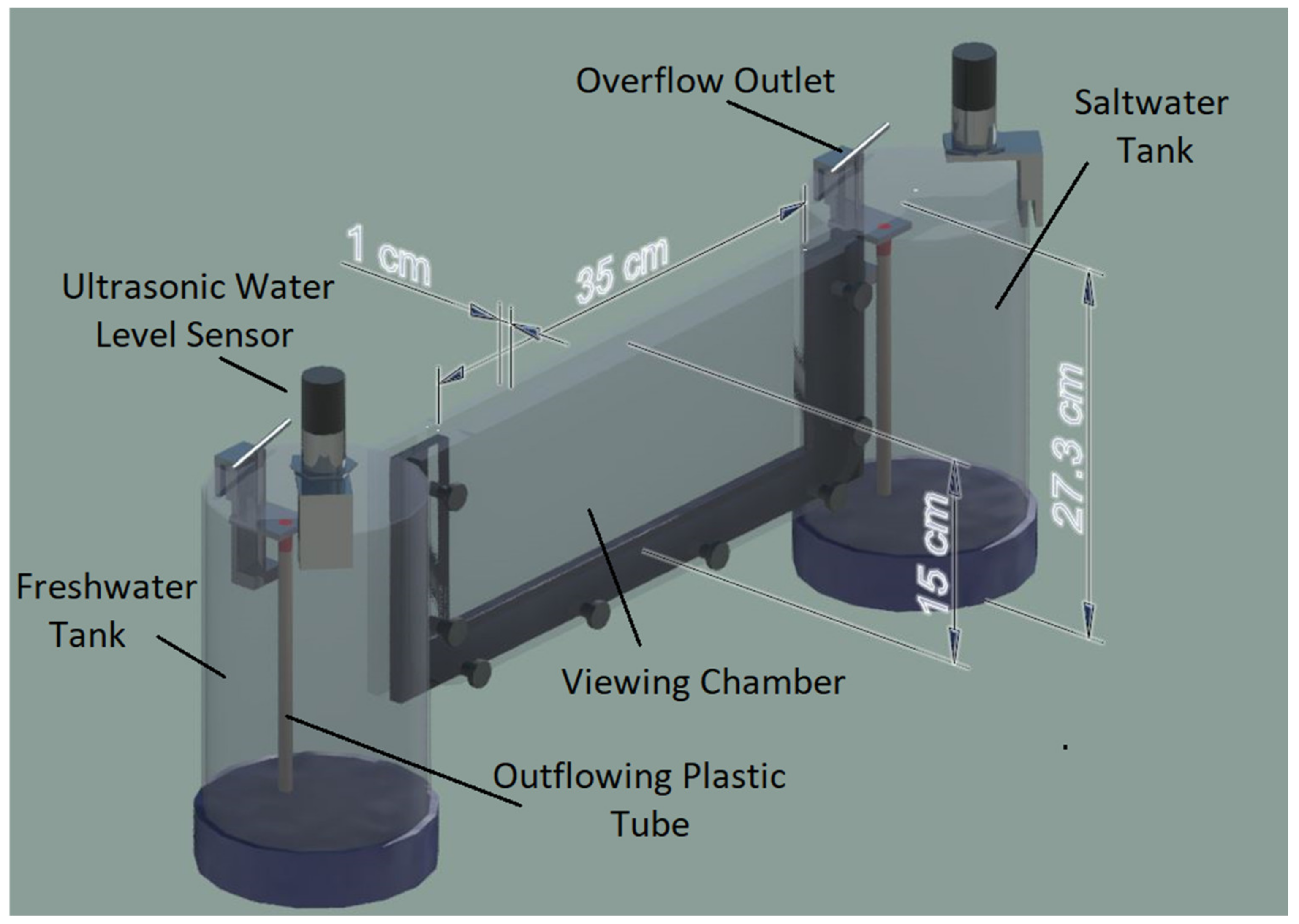
The heterogeneous experiments follow the same methodology as in Robinson et al. [34]. The methodology will be described very concisely for brevity purposes. The setup consists of a clear Perspex central chamber room of dimensions (Length × Height × Depth) 0.38 m × 0.15 m × 0.01 m, which is filled with porous media and flanked by two side-tanks filled with fixed-head freshwater and dyed seawater, both acting as boundary conditions (Figure 1). Two LED lights were used to provide the illumination, and a diffuser was placed at the back of the central chamber. The experimental procedures involve a calibration process where the porous media is flooded with saline water of different densities. An average of 10 camera images are taken, and the light intensity for every pixel is recorded for each seawater concentration which is then correlated together using a MATLAB algorithm. Images are taken using an IDT® MotionPro X-Series high-speed camera (IDT, Pasadena, CA, USA) with 1280 × 1024 pixels. Following the calibration process, the actual experiment is carried out. Different hydraulic gradients are imposed across each aquifer (dH = 6 mm, dH = 4 mm and dH = 5 mm) and images are captured during both advancing and receding saltwater wedge conditions. The experimental time for each hydraulic gradient is 50 min; this time is enough to reach the quasi steady-state condition of the saline wedge. Images are taken every 30 s to record the transient advancement/treatment of the saline wedge. Full details of the process are described in Robinson et al. [20,34].
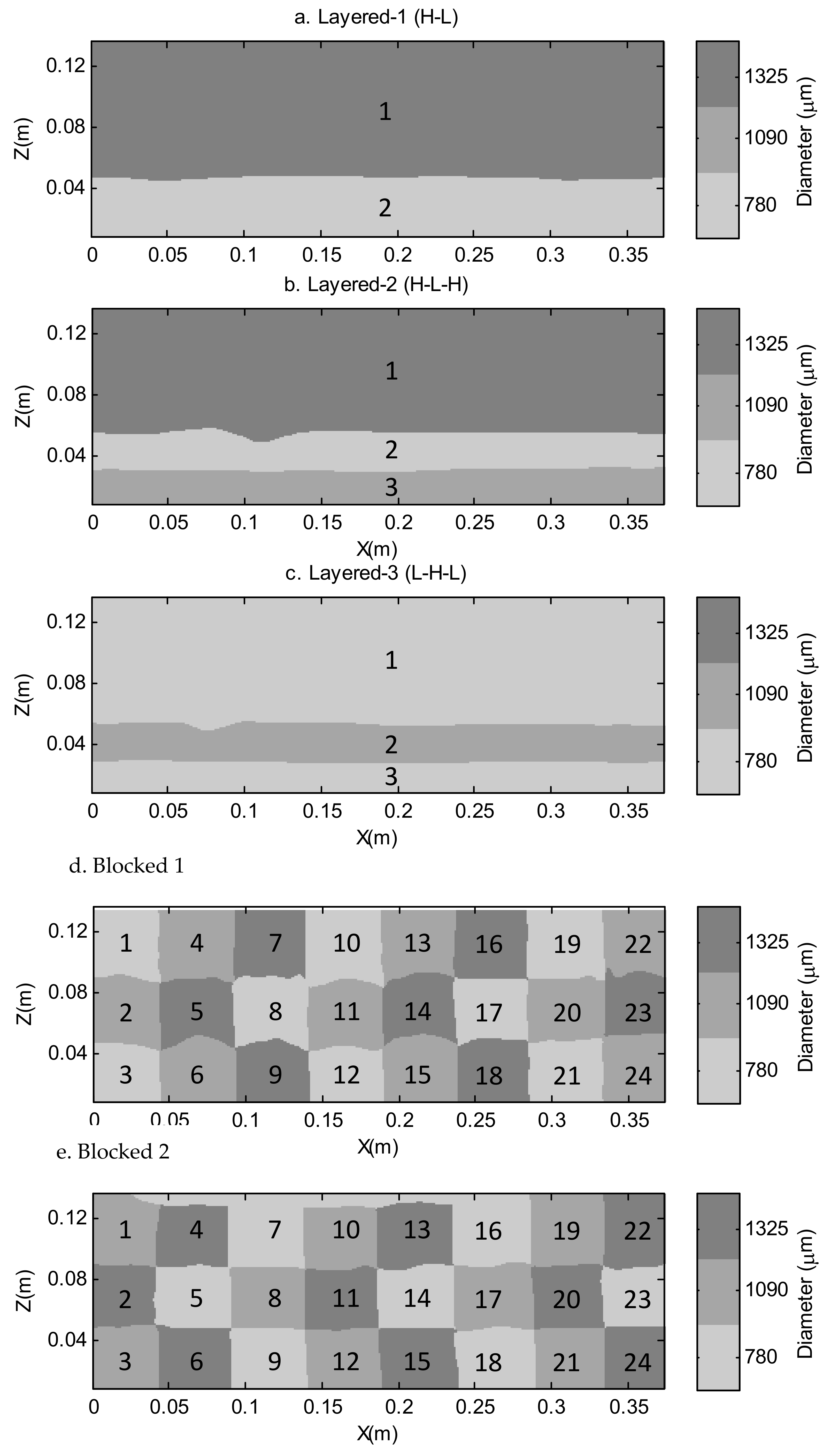
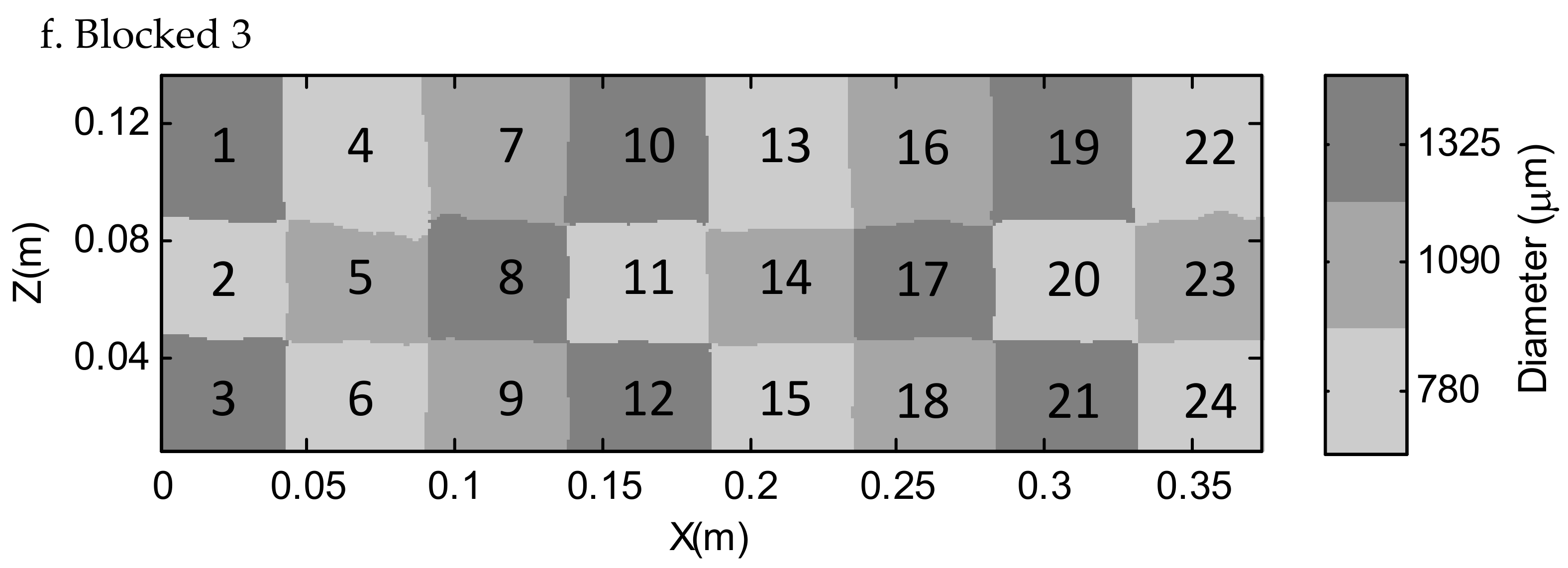
The SWI dynamics are quantified using toe length (TL), the width of the mixing zone (WMZ), and the angle of intrusion (AOI). Each experimental case includes at least two different glass bead diameters to provide variations in permeability within the synthetic aquifer. Three different bead diameters of 780 µm, 1090 µm, and 1325 µm are used to construct the heterogeneous cases. The test cases are designed to reflect increasing orders of heterogeneity, beginning with horizontally stratified layers and adding further heterogeneity to both vertical and horizontal directions using a regularly blocked style configuration. In this study, three layered and three blocked cases were tested to assess the effect of structured heterogeneity on SWI wedge dynamics. The structured heterogeneous configurations for the layered and blocked cases are shown in Figure 2, respectively. Each test case is referred to by the type of heterogeneous structure and the test number, e.g., Layered-1, Layered-2, Blocked-1, etc. Individual layers or blocks were identified using a numbering system that follows a standard pattern: starting at the top left corner and increasing from top to bottom, then left to right. This numbering system is referred to extensively in the analyses sections, which includes the quantification of intrusion parameters within specific permeability zones in the aquifer. For example, referring to the angle of intrusion of the saltwater–freshwater interface in block 20 of the first Blocked test would be equivalent to Blocked-1 AOI20. The grayscale colourmaps in Figure 2 represent the spatial distribution of the glass bead diameters within the synthetic aquifer. Hence, the boundaries between adjacent bead diameters (or permeability boundaries) appear uneven and deviate from the theoretical structure. This is due to difficulties encountered during the bead packing stage.
The structures of the heterogeneous cases are designed to provide information on the effects of a wide range of heterogeneous characteristics on SWI hydrodynamics. The Layered cases involved investigating the effects of heterogeneity in only one axis, reflecting typical (but idealised) conditions observed in sedimentary depositions. Layered-1 is the most simple form of heterogeneous structure, consisting of two permeability layers. The permeability interface between the 1325 µm layer and the 780 µm layer is replicated in the Layered-2 case, but an additional layer is added to the bottom of the aquifer. This allows the effect of different numbers of layers to be observed, as well as the effect of different flow fields on the wedge dynamics across similar permeability boundaries. Furthermore, the effect of layer thickness could be interpreted from the different thicknesses of layer 2. The Layered-3 case contains the same permeability boundary in layers 1 and 2 as that of the bottom two layers in the Layered-2 case, which allows the effect of layer depth on the same permeability boundary to be assessed. For the purposes of this study, the Layered-3 case can be thought of as the opposite of the Layered-2 case. The Layered-2 case contains a low permeability layer sandwiched between two higher permeability layers, indicated by the abbreviation H-L-H in Figure 2b. Conversely, the Layered-3 case has a high permeability layer sandwiched between two low permeability layers (L-H-L). Therefore, the Layered-3 case structure allows for the comparison of heterogeneous effects in effectively opposing flow fields.
The blocked cases are designed to investigate the effects of heterogeneity along the vertical and horizontal directions. The heterogeneous structure involves dividing the aquifer into small blocks with differing bead diameters. The blockwide pattern is consistent between test cases so that the global flow field remains similar throughout the aquifers. This allows for an initial comparison between similar permeability boundaries and dynamics within specific blocks. Furthermore, the effect of block location with respect to the saltwater–freshwater interface can be assessed.
3. Numerical Modelling Approach
The numerical simulations were conducted using SUTRA [35]. SUTRA is a finite element model for modelling saturated/unsaturated groundwater flow problems, including those with variable density. The model is widely used in numerous studies for modelling seawater intrusion problems, such as Robinson et al. [20,34] and Etsias et al. [21,22,23,24].
The numerical model consisted of a rectangular domain of the same dimensions as the central viewing chamber in the experimental tank. The element size of 1.27 mm was found to be optimal for the accurate determination of WMZs and met the Peclet criteria. Element size was chosen based on a mesh convergence study to show no change in the dispersion zone between fresh and seawater. Both the longitudinal and transverse dispersivity were obtained through a trial-and-error process [20] and fell within the range specified by Abarca and Clement [36]. The element size of the mesh and dispersivity values provided numerical stability by meeting the criterion of the Peclet number [35]. A freshwater (C = 0) hydrostatic boundary condition was forced on the left side boundary, and a hydrostatic saltwater (C = 100%) boundary condition was applied to the right side.
Different hydraulic gradients were applied into the system by setting head differences of dH = 6, 4, 5 mm between the freshwater and seawater fixed boundaries. These hydraulic gradients agree with those measured at some field sites [37]. The simulation time for each head difference or hydraulic gradient was 50 min, as in the experiment. The model input parameters are summarised in Table 1.
4. Results
To provide a sound comparative discussion of the changes to TL, WMZ, and AOI, the 1090 µm homogeneous case was chosen as the reference case to compare with all heterogeneous results. A comparison of experimental results to numerical simulations is presented throughout the results section.
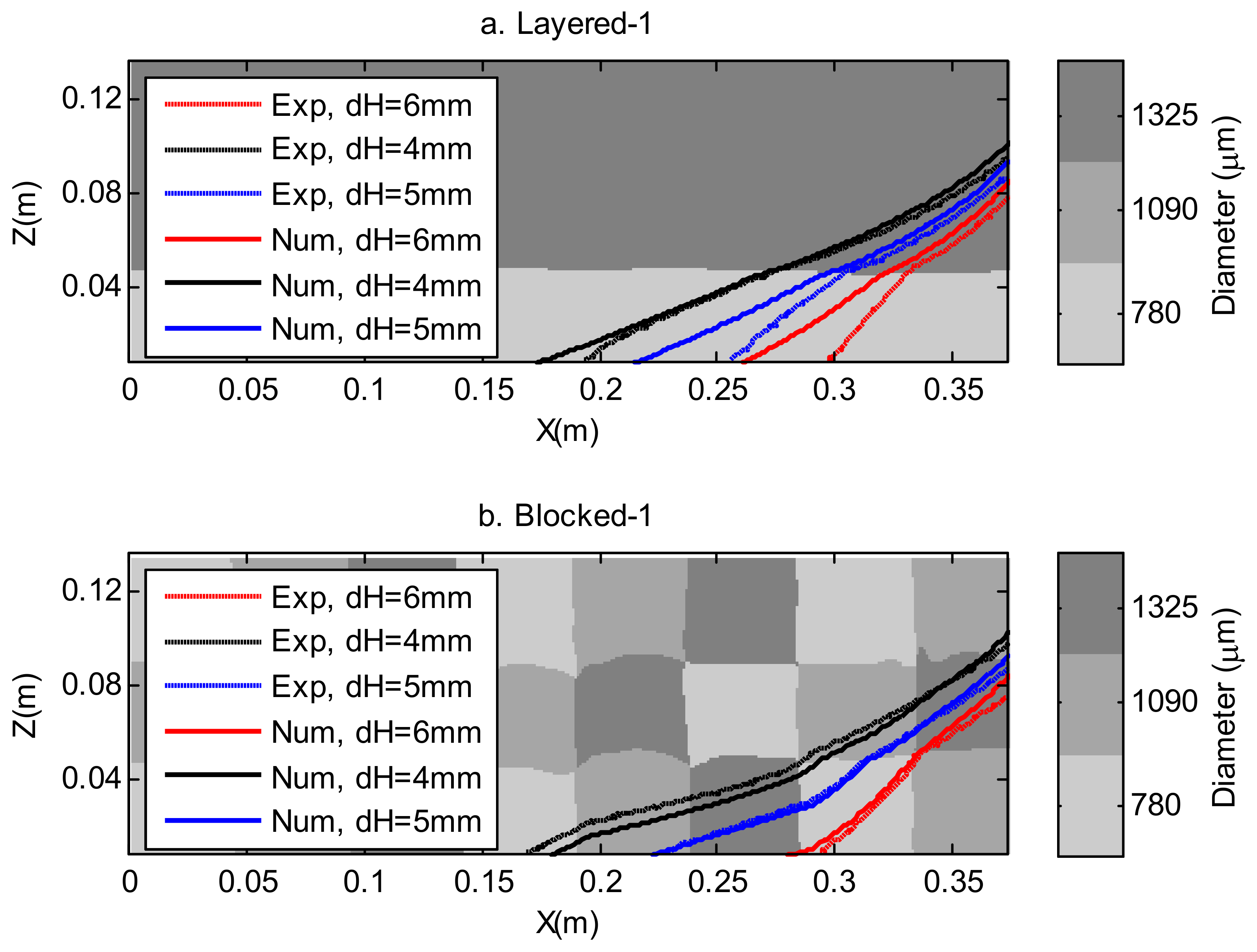
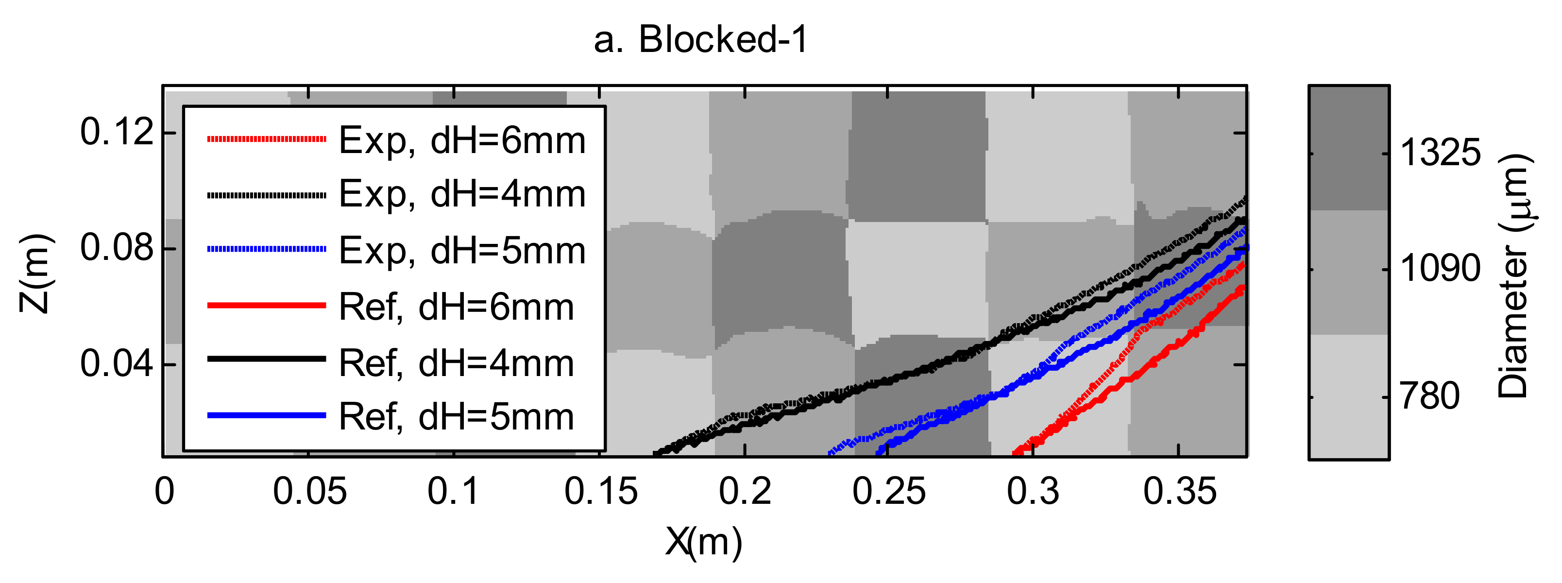
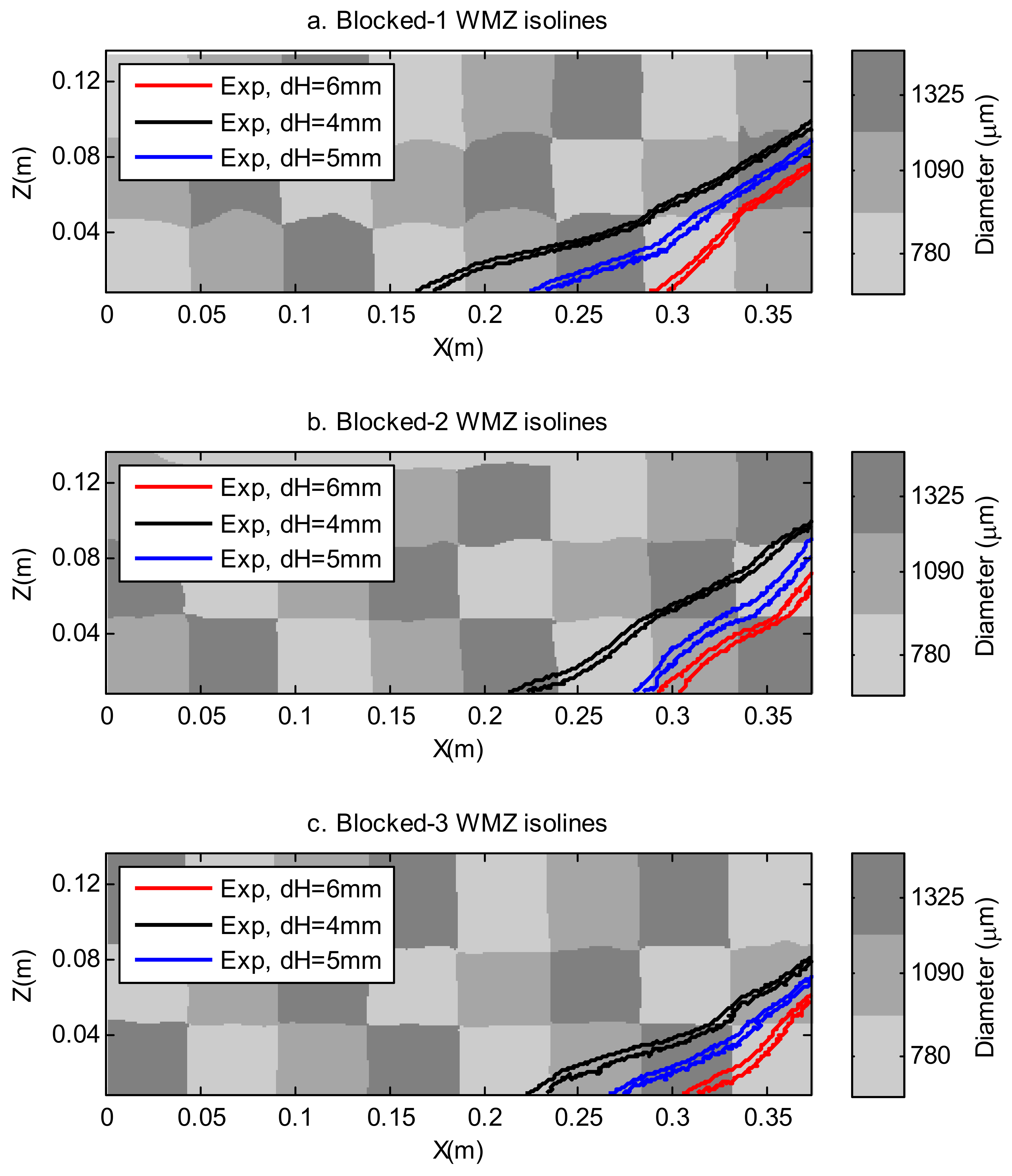
As discussed in the experimental methodology section, the steady-state condition is a quasi-steady-state where no significant change in TL is observed. The TL is determined using the 50% saltwater concentration isoline, which is also used as an indicator of the shape of the saltwater–freshwater interface. Figure 3 show the experimental and numerical steady-state saltwater 50% isolines for the Layered-1 (H-L) and Blocked-1 cases. The isolines are plotted on top of a grayscale colourmap depicting the spatial variation of the different bead diameters. As in the homogeneous results [20], a decrease in the freshwater head prompts the saltwater wedge to intrude further into the aquifer and vice versa. There is a clear change in the gradient of the saltwater–freshwater interface at the boundary of the two contrasting permeability layers in Figure 3a. This gradient change is due to the refraction of streamlines caused by the different flow field velocities within the two different permeability zones, which is a well-documented process occurring in stratified aquifers (e.g., [9,23,38,39]). The numerical results generally overpredict the TL of the experimental results. This was mainly attributed to the less pronounced gradient change when transitioning across permeability boundaries, particularly evident in the Layered-1 case (Figure 3). This effect was also observed and discussed in Robinson et al. [20], where smaller differences in intrusion parameters were recorded between the different bead diameter classes.
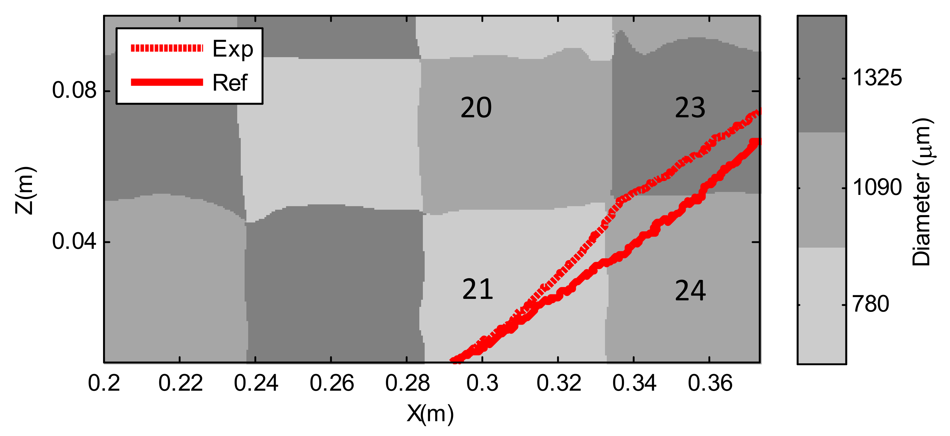
The Blocked-1 numerical results better reflect the experimental results when compared to the Layered-1 results, as shown in Figure 3. This was attributed to the saltwater wedge existing primarily in 1090 µm and 1325 µm bead diameter blocks, which have a lower permeability contrast than that of the Layered-1 case. There was only one 780 µm block (location no. 21) directly affecting the saltwater wedge in the Blocked-1 case. The gradient changes of the numerical saltwater–freshwater interface at the boundaries of this block were larger compared to the Layered-1 case, whereas the experimental results show similar gradient changes. The effect of the high permeability block (location no. 18) adjacent to block 21 was to increase the gradient of the numerical interface in block 21. The effect of surrounding permeability boundaries on the saltwater–freshwater interface is discussed further later herein.
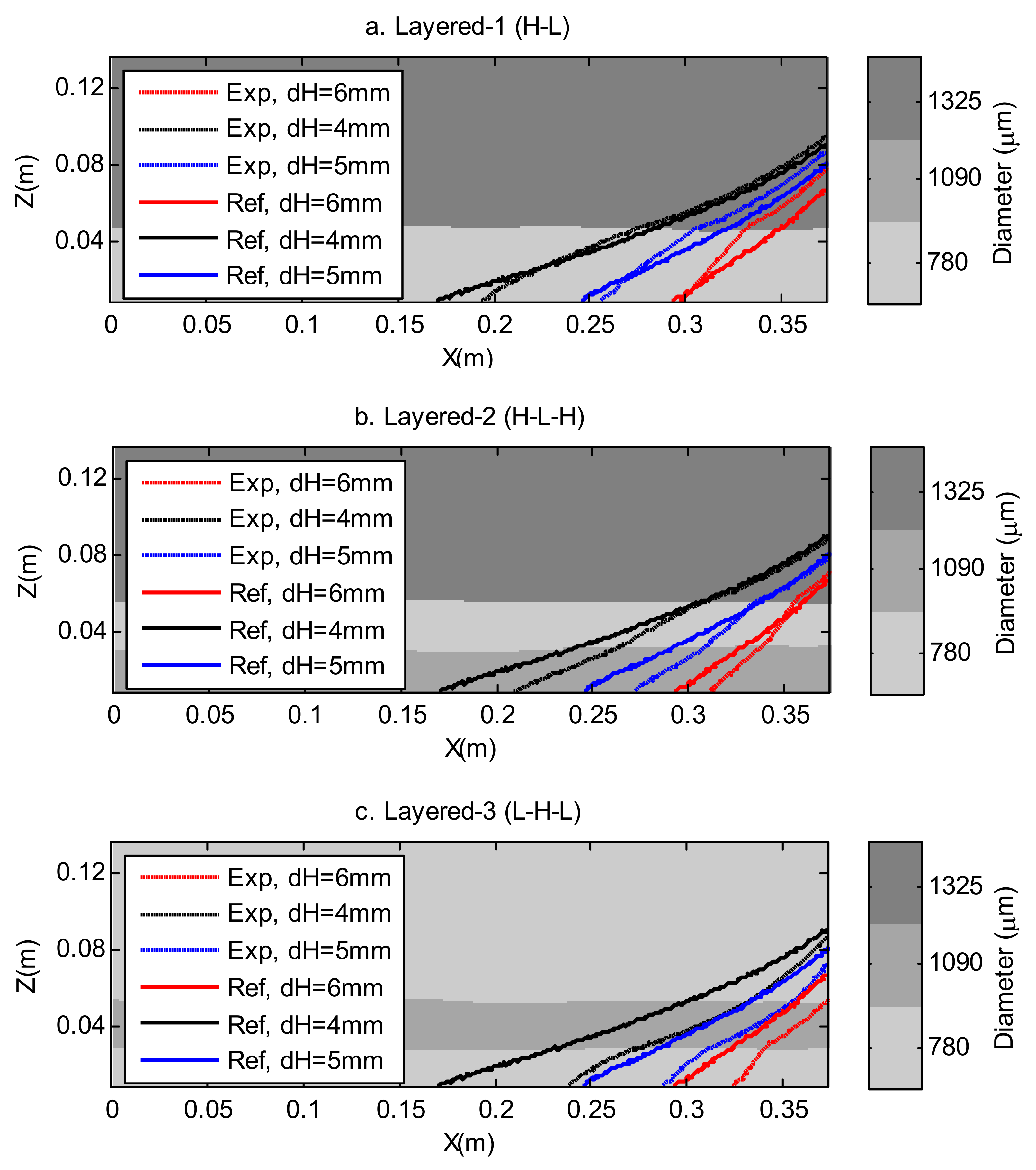
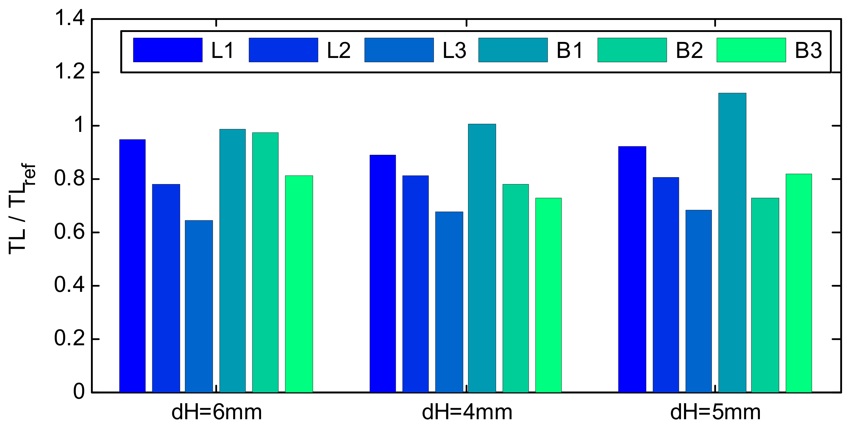
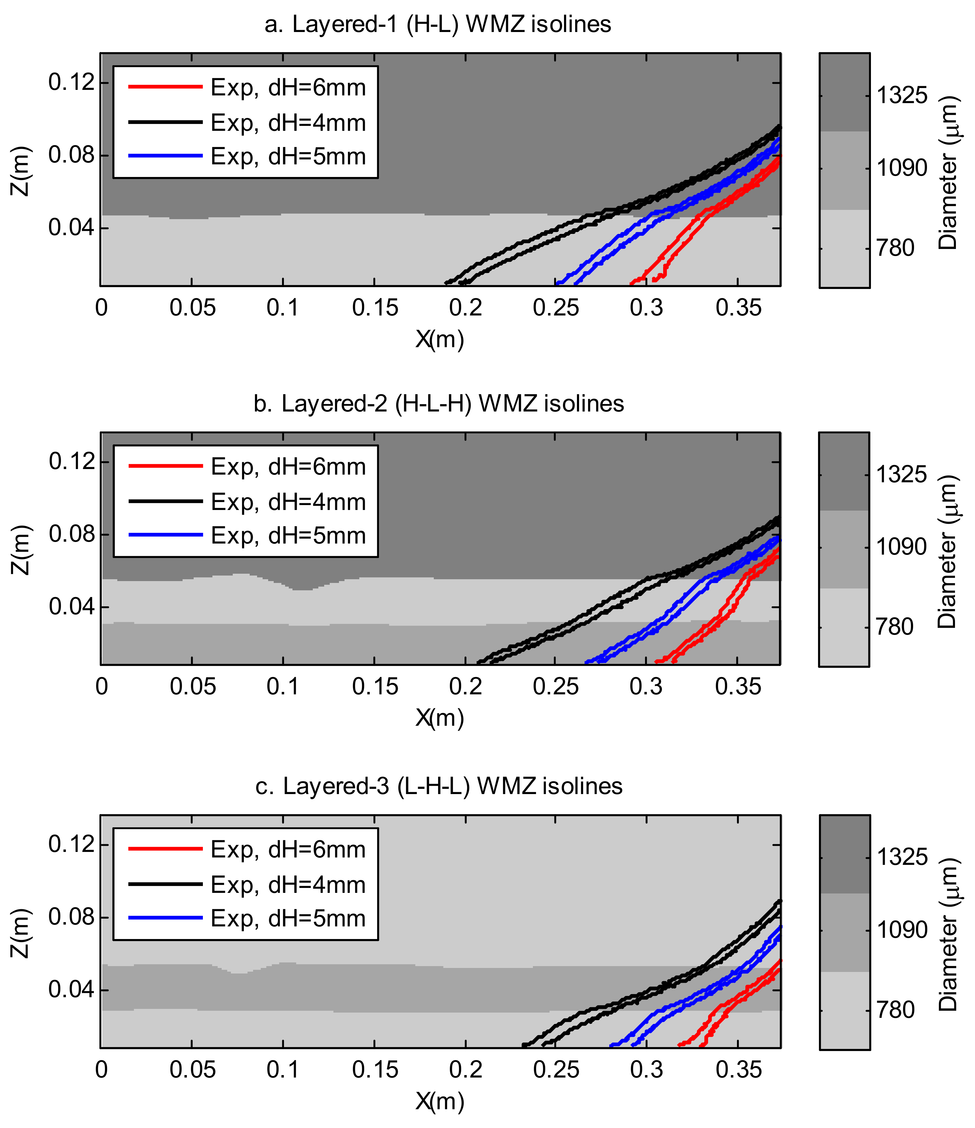
Figure 4 show the comparison between the three Layered cases and the homogeneous reference case. The blocked case results are also compared to the homogeneous reference case in Figure 5. There are several observable differences between the homogeneous and structured heterogeneous cases. The inclusion of differing permeability zones acted to reduce the TL in almost all cases, as shown in Figure 6 Generally, the saltwater–freshwater interface could not ‘recover’ from the loss in intrusion length when entering and exiting a low permeability zone. In low permeability zones, the flow paths become more restricted, and the driving head needed to penetrate the zone increases, resulting in a reduction of TL in most cases. The reduction in TL can also be interpreted by the change in WMZ across permeability layers, as shown in Figure 7. When entering a low permeability zone (middle layer), the streamlines diverge because of the increased dispersivity induced by the smaller bead size, and therefore the WMZ increases. This increased spreading produces a lower density contrast across the interface, which results in a retreat of the wedge toe. This trend was also identified in the numerical comparison between heterogeneous aquifers and effective homogeneous aquifers presented by Abarca [5] and Kerrou and Renard [7].
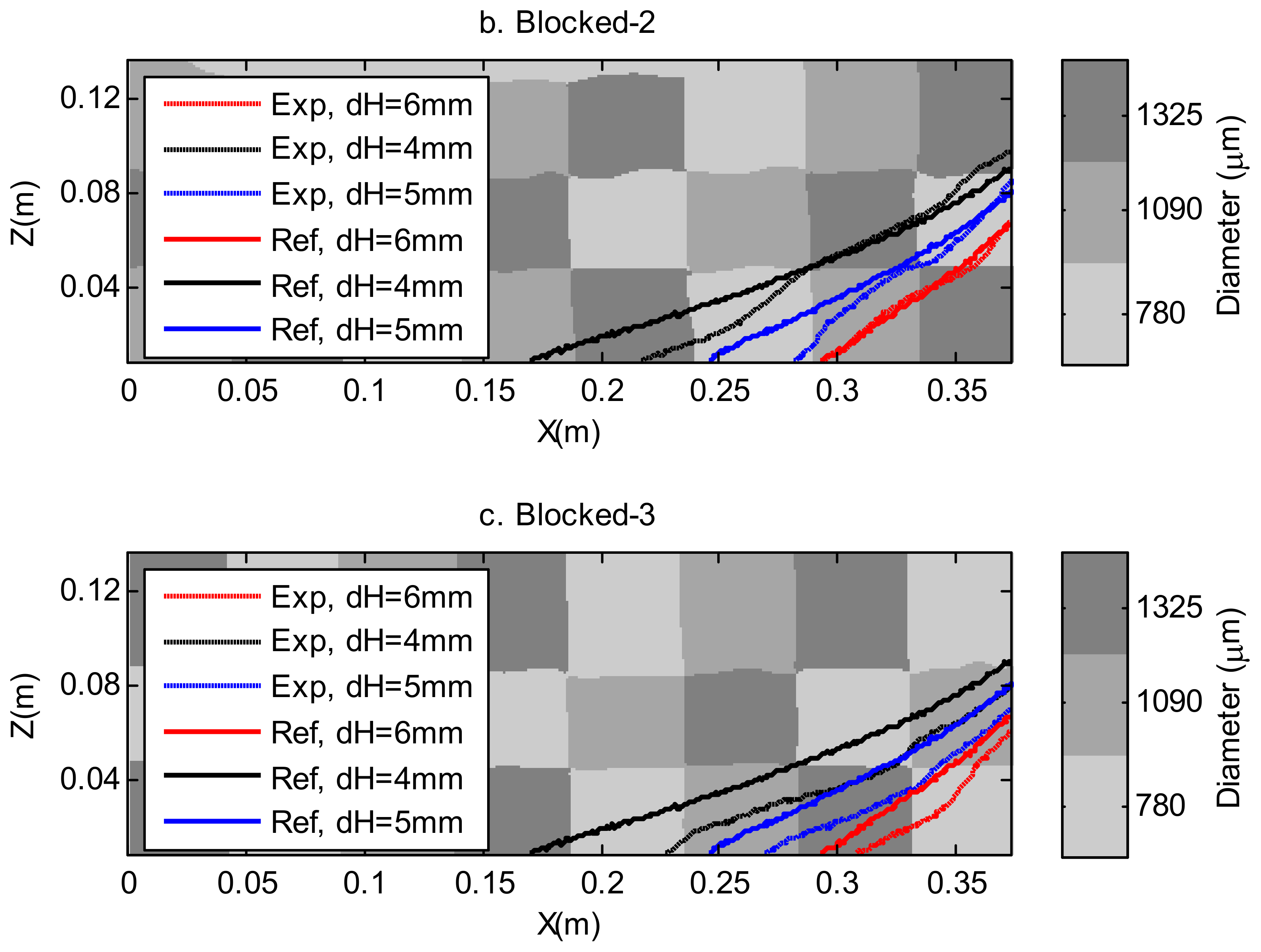
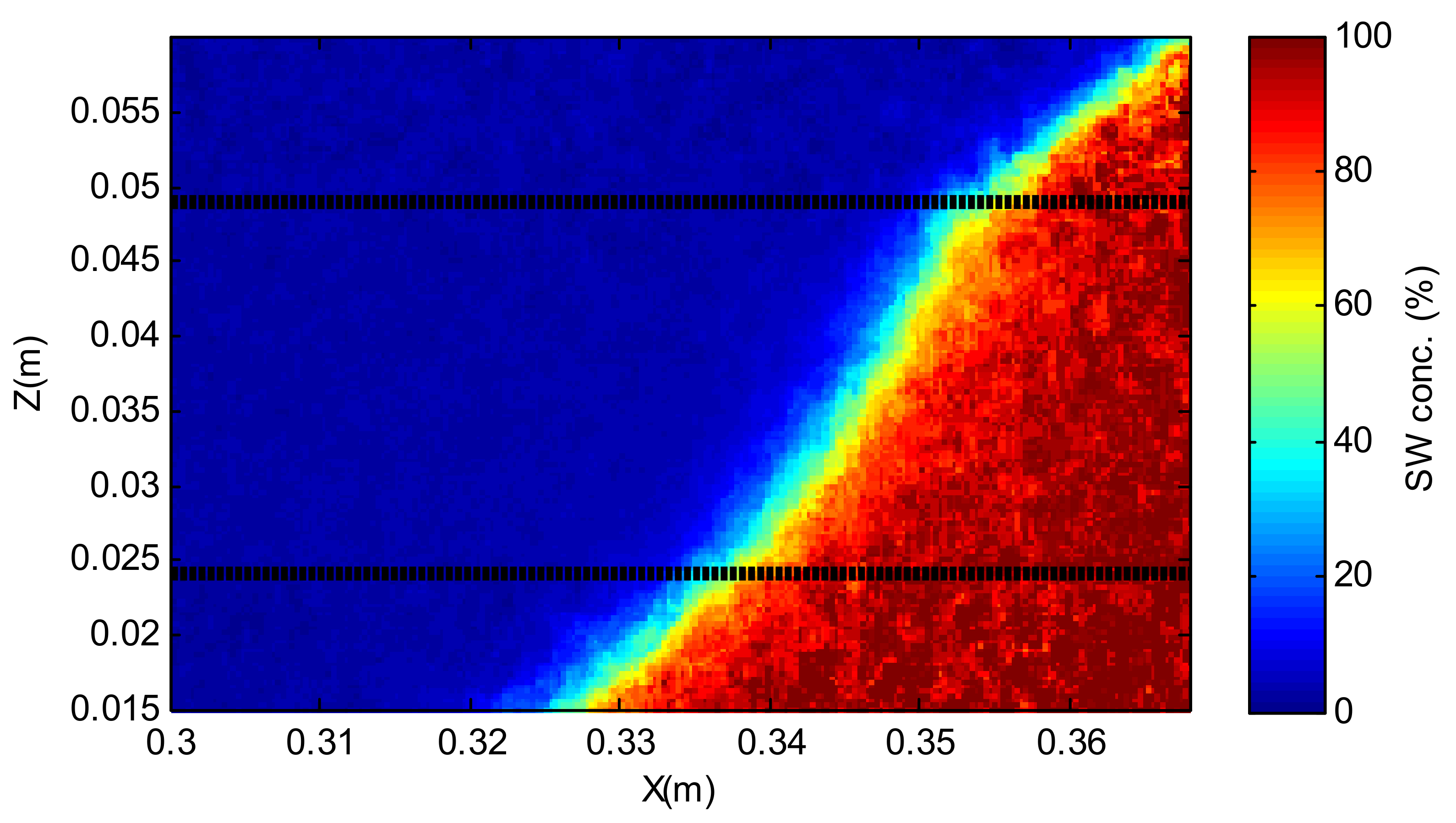
The only exception to this general trend was observed in Figure 5a and Figure 6, where the Blocked-1 heterogeneous case provided TLs similar to, and sometimes greater than, the reference homogeneous case. This case highlights the importance of the structure and connectivity of heterogeneity in SWI. The arrangement of beads in the blocked heterogeneous cases follows a consistent pattern, which allows the analysis of spatial effects while still maintaining a similar global flow pattern between cases. For the dH = 6 mm test in Figure 6 (case B1), the TLs for the experimental and reference cases are the same (TL/TLref = 1). However, on closer inspection, the shape of the wedge differs substantially, as shown in Figure 7. The vertical extension of the experimental isoline at the saltwater boundary is significantly higher than the reference case. This is due to the local structure of the heterogeneity at the saltwater boundary. Generally, water will flow along the path of least resistance. The low permeability Zone 21 provides a more restricted path to the intruding saltwater wedge. The preferred flow path is through Zones 20 and 23, as they consist of higher permeability media. However, in order to take this route, the denser saltwater has to compete against buoyancy effects and the opposing freshwater flow. This results in the saltwater wedge moving into the low permeability zone (Zone 21). The low permeability zone (Zone 17) channels the freshwater flow through the underlying high permeability zones (Zones 15 and 18). This results in a significant freshwater flow through Zone 21, which further impedes the intrusion of the wedge. The restricted transverse movement of the wedge then forces the saltwater–freshwater interface in the higher permeability zone upward (Zone 23) at the saltwater boundary, such as the effect of water being held back by a semi-permeable dam. This process is also observed in Figure 8.
In their numerical study, Kerrou and Renard [7] also observed that the increased dispersion in the heterogeneous media tended to rotate the saltwater wedge, reducing the TL and increasing the vertical extension at the saltwater boundary. Likewise, Houben et al. [10] found that aquifer heterogeneity affects the shape of the seawater–freshwater interface and the geometry of the saline water wedge. For all cases investigated here, the heterogeneity near the saltwater boundary had a significant impact on the shape of the saltwater wedge and intrusion length.
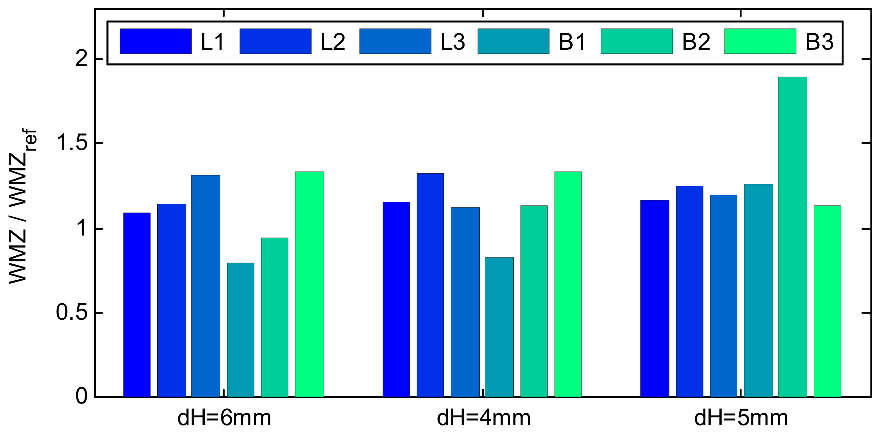
Test cases with predominantly low permeability zones at the saltwater boundary, as in Figure 3c and Figure 4c, show an overall decrease in TL and vertical extension at the seawater boundary when compared to other heterogeneous cases. The location of the low permeability zones, as well as the thickness, plays a significant role in saltwater wedge shape and intrusion dynamics. For example, Layered-1 (Figure 4a) contains a low permeability layer twice as thick as Layered-2 (b), but the TL is 13% larger (on average) for the Layered-1 case. The presence of a high permeability layer along the bottom of Layered-2 introduces an additional permeability interface and subsequent flow refraction, which increases WMZ. Figure 9 show the WMZs for the structured heterogeneous cases normalised to the reference homogeneous case. The WMZ value for Layered-2 (L2) is consistently larger (up to 20%) than the Layered-1 (L1) case. The faster-flowing freshwater in the underlying high permeability layer drives the dispersive flux along the interface, which results in a widening of the mixing zone and subsequent reduction in TL.
In general, the saltwater wedge WMZ increases in the presence of heterogeneities when compared to homogeneous media. This is true for the majority of the structured heterogeneous cases in this study, as shown in Figure 9. However, the Blocked-1 (B1) and Blocked-2 (B2) dH = 6 mm cases produced WMZs less than the reference homogeneous case. These lower WMZs correlate well with the corresponding TLs presented in Figure 6, which are large (almost equivalent to the reference case) compared with the other heterogeneous cases. The 25% and 75% concentration isolines used to determine the WMZs are shown in Figure 10 and Figure 11 for layered and blocked cases, respectively. The Blocked-1 dH = 4 mm case in Figure 11a show a stepped profile of the saltwater–freshwater interface around the low permeability zone located at its midpoint (Zone 17). This is due to the increased freshwater flow in the high permeability zones on the landward side (Zones 11, 14, 15, and 18). In fact, the only low permeability zone encountered by the interface is at the toe position, which the WMZ calculation is not likely to take into account (between 0.2 and 0.8 of TL). Therefore, it is reasonable that the WMZ for this case is small as the interface is not directly in contact with a lower permeability, high dispersion zone. This reinforces the general concept that, under the same head boundary conditions, more mixing results in lower TLs.
For the Blocked-2 case, a large increase in WMZ was observed for the dH = 5 mm test, as shown in Figure 9. On closer inspection of the concentration isolines in Figure 11b, it is clear that the low permeability zone adjacent to the saltwater boundary is the dominant contributing factor for the large WMZ.
Lu et al. [29] observed in their study that for the case where a low permeability layer is sandwiched between two higher permeability layers, the WMZ in the middle layer increased with decreasing freshwater head. A similar trend is observed in Figure 9 for the Layered-2 case (H-L-H). The WMZ in the middle layer was 24% greater for the dH = 4 mm case compared to the dH = 6 mm case. For the Layered-3 (L-H-L) case, the WMZ reduced by 11% for the dH = 4 mm case compared to the dH = 6 mm case.
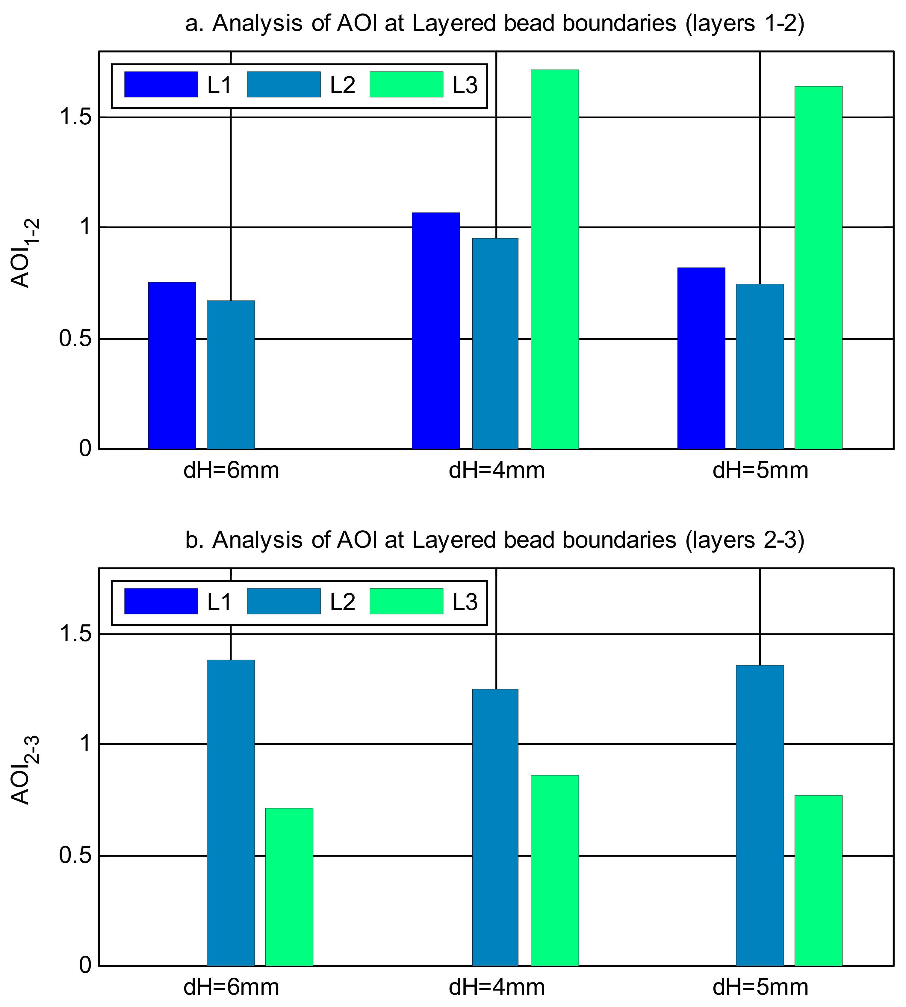
The refraction of concentration isolines at permeability boundaries was quantified using the AOI parameter. Figure 12 show the relative change in AOI, or saltwater–freshwater interface refraction factor, between layers 1 and 2 (AOI1−2 = AOI1/AOI2) and layers 2 and 3 (AOI2−3) for the layered cases. Where data appears missing from the plots, this indicates that the isoline was not present in the layer (e.g., Figure 12a L3 dH = 6 mm). It is important to note that the AOI parameter was calculated with respect to the horizontal plane. Therefore, a value of AOI1−2 < 1 means that the angle of the wedge is more vertical in layer 2 compared to layer 1, while an AOI1−2 > 1 equates to a shallower gradient in layer 2. When AOI1−2 = 1, there was no change in the saltwater wedge gradient between layers 1 and 2.
In general, the saltwater isolines became steeper when transitioning from a high permeability to a low permeability layer and vice versa. For example, the Layered-2 case (L2) in Figure 12a show AOI1−2 values consistently below 1, meaning that the gradient of the saltwater wedge is larger in layer 2 (780 µm) than in layer 1 (1325 µm). The reverse trend is also observed in Figure 12b for the Layered-2 case, where the AOI2−3 values equate to a more shallow gradient in layer 3 (1090 µm) compared to layer 2 (780 µm). This corresponds well with the TL results presented in Robinson et al. [20], which showed a reduction in intrusion length for lower permeability media under the same head boundary conditions. This trend is generally present in the other layered cases. An exception can be observed in the dH = 4 mm Layered-1 (L1) case in Figure 12a, where AOI1−2 = 1.07. Although a steeper interface angle is expected in layer 2, the isoline is significantly curved (Figure 4a), which reduces the gradient of the straight line used to determine the angle of intrusion.
At longer intrusion lengths (lower dH tests), the relative AOI change observed across permeability boundaries generally decreased. This is particularly evident from Figure 12b, where the AOI ratios were generally closer to 1.0 for the dH = 4 mm cases compared to the other head difference cases. The reverse is true for shorter intrusion lengths. This trend was also observed in the numerical results (Figure 3).
Within the structure of the three layered cases, there are similar permeability boundaries. For example, both the Layered-1 and the Layered-2 cases contain a 1325 µm layer overlying a 780 µm layer. Figure 12a show that the change in AOI across this permeability boundary is similar between these two layered cases for all head differences. However, the Layered-2 (L2) AOI1−2 results are consistently lower (avg. 9%) than the results from the Layered-1 (L1) case. A closer inspection of the individual L1 and L2 AOIs, presented in Table 2, reveals that the upper layer AOI1 values (1325 µm) were practically the same for dH = 4 mm and dH = 5 mm. Therefore, the discrepancy in AOI1−2 results are primarily due to the larger AOI2 observed in the lower layer (780 µm) for the Layered-2 case. This indicates that the refraction of the saltwater–freshwater interface at permeability boundaries is not entirely dependent on the relative permeability magnitudes of the two layers and approach angle in the upper layer. The difference in overall structure between the two cases is mainly due to the thickness of the low permeability layer and the addition of an underlying high permeability layer in the Layered-2 case. The results indicate that thinner layers have more impact, across their depth, on the refraction of the saltwater–freshwater interface at permeability boundaries. Although not highlighted directly in the analysis of layer thickness presented in Lu et al. [29], their numerical results show a similar trend for thinner layers.
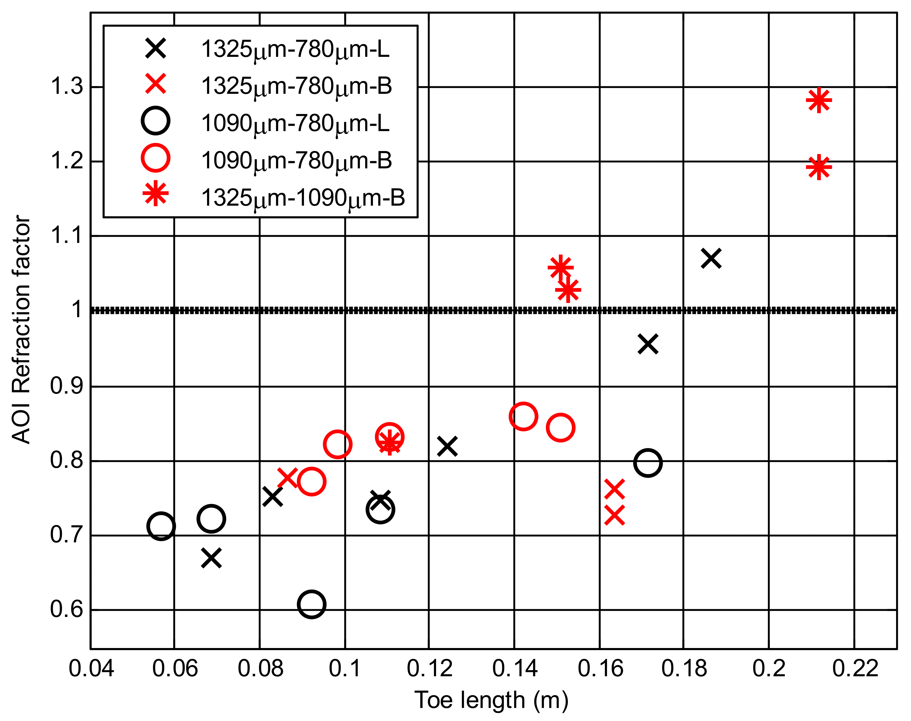
In an attempt to assess the effect of the additional permeability layer in the Layered-2 case over the Layered-1 case, similar permeability boundaries were identified and analysed in the blocked cases. With the distinctly different flow fields, the comparison cannot be considered as like for like but it may give an indication of how significant the wider flow field is on the interface. Figure 11b show the dH = 4 mm saltwater isolines passing through similar permeability boundaries at two locations; where AOI22−23 = 0.76 and AOI20−18 = 0.73. These values are significantly lower than the results from the equivalent Layered-2 test shown in Figure 12a (AOI2−3 = 96). Therefore, the flow field around the saltwater–freshwater interface plays a significant role in the refraction of the interface across permeability boundaries. Simmons et al. [2] noted that heterogeneity could perturb flow and transport over various length scales, which are often difficult to determine. The advantage of the regular structure of the Blocked cases is that the saltwater–freshwater interface refraction can be assessed across similar permeability boundaries, for similar global flow fields, at various intrusion lengths. Therefore, no matter where the permeability boundary occurs in the domain, the local flow field around the boundary will be similar between test cases. Figure 13 show the saltwater–freshwater interface refraction factor across the three possible permeability boundaries for both the layered and blocked cases. The refraction factor values are plotted against the corresponding TLs for each interface to highlight the observation discussed earlier; at longer intrusion lengths, the interface refraction across permeability boundaries decreases. The thick dashed line indicates the value at which no interface refraction occurs. Values above this line correspond to the interface becoming shallower after transitioning across the permeability boundary. This region is dominated by the refraction factor values across the boundary between the 1325 µm to 1090 µm bead size. The results of the homogeneous tests presented in Robinson et al. [20] show a similar trend, where AOIs for the 1090 µm tests were generally smaller and had longer TLs than the 1325 µm tests. Furthermore, for the Layered cases, the general tendency towards no refraction as TL increases is stronger for the 1325–780 µm boundary compared to the 1090–780 µm boundary. Conversely, the blocked cases show little correlation in Figure 13, indicating that an additional factor contributes to the refraction of the saltwater–freshwater interface in more complex heterogeneous formations.
The curved nature of the saltwater–freshwater interface, particularly evident in Figure 3 for the reference case, could play an important role in determining refraction at permeability boundaries. The slope of the saltwater–freshwater interface generally decreases with depth, indicating that the depth of the permeability boundary within the aquifer would have an effect on the refraction. The Layered-2 and Layered-3 cases contain a similar permeability boundary (1090–780 µm) but at different depths within the aquifer. The AOIs for each layer are presented in Table 2. It is interesting to note that the AOIs for the 1090 µm layer for both layered cases were similar, despite having different aquifer depths. However, the 780 µm layer AOIs differ considerably with aquifer depth. The AOI1 for the Layered-3 case (uppermost layer) is significantly larger than AOI2 for the Layered-2 case (middle layer), which in turn is larger than the AOI3 for the Layered-3 case (bottom layer). This trend emulates the curved shape of the saltwater–freshwater interface in homogeneous cases. Further evidence for the effect of aquifer depth on saltwater wedge interface refraction was observed in the Layered-3 case where, for the same permeability boundary, the AOI1 remained consistently larger than AOI3 for all head difference cases tested. This section identified several effects of heterogeneity on steady-state SWI and attempted to quantify trends from the results of the experimental programme. It is clear that the complex effects induced by heterogeneity were not sufficiently isolated within the limited number of experiments that time permitted in this study. However, the results can be used as a guideline to design a more robust experimental programme to target specific heterogeneous effects, which can be analysed and quantified in more detail using the same image analysis methodology.
5. Conclusions
An experimental study of the hydrodynamic effects of heterogeneity on SWI was conducted. The high temporal and spatial resolution of the image analysis procedure allowed for the observation and quantification of transient SWI parameters at a laboratory scale. Several different types of heterogeneous aquifers were tested, starting with layered and increasing in complexity to blocked cases. The heterogeneous results were compared to a reference homogeneous case and result from numerical modelling. The main findings of the study were:
- For the test cases analysed in this study, wedge toe length generally decreased under heterogeneous conditions, while the freshwater–saltwater dispersion or mixing zone generally increased when compared to the homogenous reference case. This is in agreement with previous numerical studies of random heterogeneous aquifers;
- The saltwater–freshwater interface shows a distinct gradient change across differing permeability boundaries. This was attributed to streamline refraction, which caused the angle of intrusion to increase when transitioning from high to low permeability zones and vice versa. The refraction also affected the mixing zone, where additional spreading was also observed when transitioning from high to low permeability zones and vice versa;
- Predominantly low permeability zones at the saltwater boundary reduced the toe length and vertical extensions of the wedge. High permeability zones near the saltwater boundary caused channeling of flow into the aquifer and facilitated intrusion. It is therefore important to consider the structure of the heterogeneity as well as the relative permeability;
- For the Layered-2 case (H-L-H), the increased spreading in the middle layer caused by flow refraction was enhanced at low hydraulic gradients. For the Layered-3 case (L-H-L), a reduction in hydraulic gradient produced lower dispersion or mixing zone in the middle layer;
- The relative change in the angle of intrusion across permeability zones is not solely dependent on relative permeability but also depends on the hydraulic gradient, depth in the aquifer, zone thickness, and surrounding permeability distribution.
Some of the hydrodynamic effects of heterogeneity observed in this study were documented in other published literature, while others are yet to be observed. There were difficulties in isolating individual heterogeneous effects, and attempts were made to decouple the hydrodynamics for analysis with some success. At the very least, this study provides insight into the general processes of SWI in heterogeneous aquifers and could be used as a basis for defining conceptual models of real-world systems. It also highlights the capabilities of the image analysis procedure to capture small perturbations, particularly within the mixing zone, that are essential for defining the aquifer flow regime and predicting the location of the saltwater–freshwater interface. The results from this study could be used to better design future experimental cases to target individual heterogeneous effects and to quantify these effects by taking advantage of the high temporal and spatial resolutions provided by the automated image analysis procedure.
Author Contributions
Conceptualization, G.R., G.H. and A.A.; methodology, G.R., G.H. and A.A.; software, G.R.; validation, G.R., A.A. and G.H.; formal analysis, G.R.; investigation, G.R. and G.E.; resources, G.H. and A.A.; data curation, G.R.; writing—original draft preparation, G.R.; writing—review and editing, A.A., G.R., G.H. and G.E.; visualization, G.R.; supervision, G.H. and A.A.; project administration, A.A. and G.H.; funding acquisition, G.H. and A.A. All authors have read and agreed to the published version of the manuscript.
Funding
This research was funded by the Engineering and Physical Science Research Council (EPSRC) in the UK by grant number EP/R019258/1.
Institutional Review Board Statement
Not applicable.
Informed Consent Statement
Not applicable.
Data Availability Statement
Not applicable.
Conflicts of Interest
The authors declare no conflict of interest.
References
- Dagan, G.; Neuman, S. Subsurface Flow and Transport: A Stochastic Approach, 1st ed.; Cambridge University Press: Cambridge, UK, 1997. [Google Scholar]
- Simmons, C.T.; Fenstemaker, T.R.; Sharp, J.M., Jr. Variable-density groundwater flow and solute transport in heterogeneous porous media: Approaches, resolutions and future challenges. J. Contam. Hydrol. 2001, 52, 245–275. [Google Scholar] [CrossRef]
- Dagan, G. Flow and transport in highly heterogeneous formations: Conceptual uncertainty and solution for a multi-indicator permeability structure. In Calibration and Reliability in Groundwater Modelling: A Few Steps Closer to Reality (Proceedings of ModelCARE 2002, Prague, Czech Republic, 17–20 June 2002); Kovar, K., Hrkal, Z., Eds.; International Association of Hydrological Sciences: Prague, Czech Republic, 2002; pp. 95–101. [Google Scholar]
- Held, R.; Attinger, S.; Kinzelbach, W. Homogenization and effective parameters or the Henry problem in heterogeneous formations. Water Resour. Res. 2005, 41, 1–14. [Google Scholar] [CrossRef]
- Abarca, E. Seawater Intrusion in Complex Geological Environments. Ph.D. Thesis, Department of Geotechnical Engineering and Geo-Sciences (ETCG) Technical University of Catalonia, UPC, Barcelona, Spain, 2006. [Google Scholar]
- Bear, J.; Zhou, Q. Sea Water Intrusion into Coastal Aquifers, The Handbook of Groundwater Engineering, 2nd ed.; Delleur, J., Ed.; CRC Press: Boca Raton, FL, USA, 2007; pp. 12–29. [Google Scholar]
- Kerrou, J.; Renard, P. A numerical analysis of dimensionality and heterogeneity effects on advective dispersive seawater intrusion processes. Hydrogeol. J. 2010, 18, 55–72. [Google Scholar] [CrossRef] [Green Version]
- Ababou, R.; Al-Bitar, R. Salt water intrusion with heterogeneity and uncertainty: Mathematical modelling and analyses. Dev. Water Sci. 2005, 55, 1559–1571. [Google Scholar]
- Servan-Camas, B.; Tsain, F.T. Saltwater intrusion modelling in heterogeneous confined aquifers using two-relaxation-time lattice Boltzmann method. Adv. Water Resour. 2009, 32, 620–631. [Google Scholar] [CrossRef]
- Houben, G.J.; Stoeckl, L.; Mariner, K.E.; Choudhury, A.S. The influence of heterogeneity on coastal groundwater flow-physical and numerical modelling of fringing reefs, dykes and structured conductivity field. Adv. Water Resour. 2018, 113, 155–166. [Google Scholar] [CrossRef]
- Pool, M.; Post, V.E.; Simmons, C.T. Effects of tidal fluctuations and spatial heterogeneity on mixing and spreading in spatially heterogeneous coastal aquifers. Water Resour. Res. 2015, 51, 1570–1585. [Google Scholar] [CrossRef]
- Siena, M.; Riva, M. Groundwater withdrawal in randomly heterogeneous coastal aquifers. Hydrol. Earth Syst. Sci. 2018, 22, 2971–2985. [Google Scholar] [CrossRef] [Green Version]
- Chang, C.M.; Yeh, H.D. Spectral approach to seawater intrusion in heterogeneous coastal aquifers. Hydrol. Earth Syst. Sci. 2010, 7, 719–727. [Google Scholar] [CrossRef] [Green Version]
- Abdoulhalik, A.; Ahmed, A.A. The effectiveness of cutoff walls to control saltwater intrusion in multi-layered coastal aquifers: Experimental and numerical study. J. Environ. Manag. 2017, 199, 62–73. [Google Scholar] [CrossRef] [Green Version]
- Chang, Q.; Zheng, T.; Zheng, X.; Zhang, B.; Sun, Q.; Walther, M. Effect of subsurface dams on saltwater intrusion and fresh groundwater discharge. J. Hydrol. 2019, 576, 508–519. [Google Scholar] [CrossRef]
- Kuan, W.K.; Xin, P.; Jin, G.; Robinson, C.E.; Gibbes, B.; Li, L. Combined Effect of Tides and Varying Inland Groundwater Input on Flow and Salinity Distribution in Unconfined Coastal Aquifers. Water Resour. Res. 2019, 55, 8864–8880. [Google Scholar] [CrossRef]
- Lee, W.-D.; Yoo, Y.-J.; Jeong, Y.-M.; Hur, D.-S. Experimental and Numerical Analysis on Hydraulic Characteristics of Coastal Aquifers with Seawall. Water 2019, 11, 2343. [Google Scholar] [CrossRef] [Green Version]
- Levanon, E.; Gvirtzman, H.; Yechieli, Y.; Oz, I.; Ben-Zur, E.; Shalev, E. The Dynamics of Sea Tide-Induced Fluctuations of Groundwater Level and Freshwater-Saltwater Interface in Coastal Aquifers: Laboratory Experiments and Numerical Modeling. Geofluids 2019, 2019, 6193134. [Google Scholar] [CrossRef] [Green Version]
- Memari, S.S.; Bedekar, V.S.; Clement, T.P. Laboratory and Numerical Investigation of Saltwater Intrusion Processes in a Circular Island Aquifer. Water Resour. Res. 2020, 56, e2019WR025325. [Google Scholar] [CrossRef]
- Robinson, G.; Ahmed, A.A.; Hamill, G.A. Experimental saltwater intrusion in coastal aquifers using automated image analysis: Applications to homogeneous aquifers. J. Hydrol. 2016, 538, 304–313. [Google Scholar] [CrossRef] [Green Version]
- Etsias, G.; Hamill, G.A.; Benner, E.; Águila, J.F.; McDonnell, M.C.; Flynn, R.; Ahmed, A.A. Optimizing Laboratory Investigations of Saline Intrusion by Incorporating Machine Learning Techniques. Water 2020, 12, 2996. [Google Scholar] [CrossRef]
- Etsias, G.; Hamill, G.A.; Campbell, D.; Straney, R.; Benner, E.M.; Águila, J.F.; Flynn, R. Laboratory and numerical investigation of saline intrusion in fractured coastal aquifers. Adv. Water Resour. 2021, 149, 103866. [Google Scholar] [CrossRef]
- Etsias, G.; Hamill, G.A.; Águila, J.F.; Benner, E.M.; McDonnell, M.C.; Ahmed, A.A.; Flynn, R. The impact of aquifer stratification on saltwater intrusion characteristics. Comprehensive laboratory and numerical study. Hydrol. Process. 2021, 35, e14120. [Google Scholar] [CrossRef]
- Etsias, G.; Hamill, G.A.; Thomson, C.; Kennerley, S.; Aguila, J.F.; Benner, E.M.; McDonnell, M.C.; Ahmed, A.; Flynn, R. Laboratory and Numerical Study of Saltwater Upconing in Fractured Coastal Aquifers. Water 2021, 13, 3331. [Google Scholar] [CrossRef]
- Mehdizadeh, S.S.; Werner, A.D.; Vafaie, F.; Badaruddin, S. Vertical leakage in sharp-interface seawater intrusion models of layered coastal aquifers. J. Hydrol. 2014, 519, 1097–1107. [Google Scholar] [CrossRef]
- Dose, E.J.; Stoeckl, L.; Houben, G.J.; Vacher, H.L.; Vassolo, S.; Dietrich, J.; Himmelsbach, T. Experiments and modeling of freshwater lenses in layered aquifers: Steady state interface geometry. J. Hydrol. 2014, 509, 621–630. [Google Scholar] [CrossRef]
- Stoeckl, L.; Houben, G.J.; Dose, E.J. Experiments and modeling of flow processes in freshwater lenses in layered island aquifers: Analysis of age stratification, travel times and interface propagation. J. Hydrol. 2015, 529, 159–168. [Google Scholar] [CrossRef]
- Chowdhury, A.S.; Stoeckl, L.; Houben, G. Influence of geological heterogeneity on the saltwater freshwater interface position in coastal aquifers—Physical experiments and numerical modelling. In Proceedings of the 23rd Saltwater Intrusion Meeting, Husum, Germany, 16–20 June 2014; pp. 393–396. [Google Scholar]
- Lu, C.; Chen, Y.; Zhang, C.; Luo, J. Steady-state freshwater–seawater mixing zone in stratified coastal aquifers. J. Hydrol. 2013, 505, 24–34. [Google Scholar] [CrossRef]
- Liu, Y.; Mao, X.; Chen, J.; Barry, D.A. Influence of a coarse interlayer on seawater intrusion and contaminant migration in coastal aquifers. Hydrol. Process. 2014, 28, 5162–5175. [Google Scholar] [CrossRef]
- Guo, Q.; Huang, J.; Zhou, Z.; Wang, J. Experiment and Numerical Simulation of Seawater Intrusion under the Influences of Tidal Fluctuation and Groundwater Exploitation in Coastal Multilayered Aquifers. Geofluids 2019, 2019, 2316271. [Google Scholar] [CrossRef] [Green Version]
- Dalai, C.; Munusamy, S.B.; Dhar, A. Experimental and numerical investigation of saltwater intrusion dynamics on sloping sandy beach under static seaside boundary condition. Flow Meas. Instrum. 2020, 75, 101794. [Google Scholar] [CrossRef]
- Abdoulhalik, A.; Abdelgawad, A.M.; Ahmed, A.A. Impact of layered heterogeneity on transient saltwater upconing in coastal aquifers. J. Hydrol. 2020, 581, 124393. [Google Scholar] [CrossRef]
- Robinson, G.; Hamill, G.A.; Ahmed, A.A. Automated image analysis for experimental investigations of salt water intrusion in coastal aquifers. J. Hydrol. 2015, 530, 350–360. [Google Scholar] [CrossRef] [Green Version]
- Voss, C.I.; Provost, A.M. SUTRA: A Model for Saturated-Unsaturated, Variable-Density Ground-Water Flow with Solute or Energy Transport, 2nd ed.; USGS: Reston, VA, USA, 2010. [Google Scholar]
- Abarca, E.; Clement, T.P. A novel approach for characterizing the mixing zone of a saltwater wedge. Geophys. Res. Lett. 2009, 36, L06402. [Google Scholar] [CrossRef] [Green Version]
- Ferguson, G.; Gleeson, T. Vulnerability of coastal aquifers to groundwater use and climate change. Nat. Clim. Change 2012, 2, 342–345. [Google Scholar] [CrossRef]
- Abdoulhalik, A.; Ahmed, A.A. How does layered heterogeneity affect the ability of subsurface dams to clean up coastal aquifers contaminated with seawater intrusion? J. Hydrol. 2017, 553, 708–721. [Google Scholar] [CrossRef] [Green Version]
- Abdoulhalik, A.; Ahmed, A.A.; Hamill, G.A. A new physical barrier system for seawater intrusion control. J. Hydrol. 2017, 549, 416–427. [Google Scholar] [CrossRef] [Green Version]
Figure 1.
Three-dimensional representation of the sandbox setup.

Figure 2.
Bead size distribution for the layered (a–c) and blocked (d–f) heterogeneous configurations. The grayscale colourmap represents bead diameter, and the numbers identify the individual permeability zones for analysis.
Figure 2.
Bead size distribution for the layered (a–c) and blocked (d–f) heterogeneous configurations. The grayscale colourmap represents bead diameter, and the numbers identify the individual permeability zones for analysis.


Figure 3.
Experimental and numerical steady-state 50% salt concentration isolines for the (a) Layered-1 case and (b) Blocked-1 case at head differences, dH = 6 mm, 4 mm, and 5 mm.
Figure 3.
Experimental and numerical steady-state 50% salt concentration isolines for the (a) Layered-1 case and (b) Blocked-1 case at head differences, dH = 6 mm, 4 mm, and 5 mm.

Figure 4.
Experimental steady-state 50% salt concentration isolines for the layered cases compared to the homogeneous reference case, at head differences, dH = 6 mm, 4 mm, and 5 mm. ((a) High-Low, (b) High-Low-High, (c) Low-High-Low).
Figure 4.
Experimental steady-state 50% salt concentration isolines for the layered cases compared to the homogeneous reference case, at head differences, dH = 6 mm, 4 mm, and 5 mm. ((a) High-Low, (b) High-Low-High, (c) Low-High-Low).

Figure 5.
Experimental steady-state 50% salt concentration isolines for the blocked cases compared to the homogeneous reference case, at head differences, dH = 6 mm, 4 mm, and 5 mm. ((a) blocked group 1, (b) Blocked group 2, (c) Blocked group 3).
Figure 5.
Experimental steady-state 50% salt concentration isolines for the blocked cases compared to the homogeneous reference case, at head differences, dH = 6 mm, 4 mm, and 5 mm. ((a) blocked group 1, (b) Blocked group 2, (c) Blocked group 3).


Figure 6.
Experimental toe length ratios (TL/TLref) for comparison of heterogeneous cases to the homogeneous reference case for dH = 6 mm, 4 mm, and 5 mm.
Figure 6.
Experimental toe length ratios (TL/TLref) for comparison of heterogeneous cases to the homogeneous reference case for dH = 6 mm, 4 mm, and 5 mm.

Figure 7.
Experimental Layered-2 (H-L-H) interface showing larger mixing zone in low permeability layer.
Figure 7.
Experimental Layered-2 (H-L-H) interface showing larger mixing zone in low permeability layer.

Figure 8.
Blocked-1 50% saltwater concentration isolines with labelled permeability zones of interest near the saltwater boundary.
Figure 8.
Blocked-1 50% saltwater concentration isolines with labelled permeability zones of interest near the saltwater boundary.

Figure 9.
Experimental width of the mixing zone ratios (WMZ/WMZref) for comparison of heterogeneous cases to the homogeneous reference case for dH = 6 mm, 4 mm, and 5 mm.
Figure 9.
Experimental width of the mixing zone ratios (WMZ/WMZref) for comparison of heterogeneous cases to the homogeneous reference case for dH = 6 mm, 4 mm, and 5 mm.

Figure 10.
Experimental steady-state 25% (upper line) and 75% (lower line) salt concentration isolines 6 mm, 4 mm, and 5 mm. ((a) High-Low, (b) High-Low-High, (c) Low-High-Low).
Figure 10.
Experimental steady-state 25% (upper line) and 75% (lower line) salt concentration isolines 6 mm, 4 mm, and 5 mm. ((a) High-Low, (b) High-Low-High, (c) Low-High-Low).

Figure 11.
Experimental steady-state 25% (upper line) and 75% (lower line) salt concentration isolines for the Blocked cases at head differences, dH = 6 mm, 4 mm, and 5 mm. ((a) blocked group 1, (b) Blocked group 2, (c) Blocked group 3).
Figure 11.
Experimental steady-state 25% (upper line) and 75% (lower line) salt concentration isolines for the Blocked cases at head differences, dH = 6 mm, 4 mm, and 5 mm. ((a) blocked group 1, (b) Blocked group 2, (c) Blocked group 3).

Figure 12.
Experimental steady-state AOI ratios across bead layer boundaries for the Layered cases at head differences, dH = 6 mm, 4 mm, and 5 mm. ((a) layers 1–2, (b) layers 2–3).
Figure 12.
Experimental steady-state AOI ratios across bead layer boundaries for the Layered cases at head differences, dH = 6 mm, 4 mm, and 5 mm. ((a) layers 1–2, (b) layers 2–3).

Figure 13.
Saltwater–freshwater interface refraction across permeability boundaries for layered (black) and blocked (red) cases at corresponding TLs.
Figure 13.
Saltwater–freshwater interface refraction across permeability boundaries for layered (black) and blocked (red) cases at corresponding TLs.


Table 1.
SUTRA simulation input summary.
| Input Parameters | Value | Unit |
|---|---|---|
| Domain size, L × H | 0.38 × 0.1357 | m |
| Element size | 1.27 × 10⁻³ | m |
| Permeability: | ||
| −780 µm | 7.98 × 10⁻¹⁰ | m2 |
| −1090 µm | 1.83 × 10⁻⁹ | m2 |
| −1325 µm | 2.39 × 10⁻⁹ | m2 |
| Porosity | 0.385 | |
| Molecular diffusivity | 1.00 × 10⁻⁹ | m2/s |
| Longitudinal dispersivity | 1 × 10⁻³ | m |
| Transverse dispersivity | 5 × 10⁻⁵ | m |
| Freshwater density | 1000 | kg/m3 |
| Saltwater density | 1025 | kg/m3 |
| Dynamic viscosity | 0.001 | kg/m/s |
| Head difference, dH | 6, 4, 5 | mm |
| Simulation time | 50 | mins |
| Time step | 1 | s |
Table 2.
Angle of intrusion for each Layered case at head differences dH = 4 and 5 mm. AOI1, AOI2 and AOI3 are the angles of intrusion in layers 1, 2, and 3, respectively. Cells are colour coded to match layer bead diameter, consistent with previous Figure 2, Figure 3, Figure 4, Figure 5, Figure 10 and Figure 11 (darkest = 1325 µm, middle = 1090 µm, lightest = 780 µm).
| Layered Case | AOI1 (°) | AOI2 (°) | AOI3 (°) | |||
|---|---|---|---|---|---|---|
| dH | 4 mm | 5 mm | 4 mm | 5 mm | 4 mm | 5 mm |
| 1 | 25.87 | 30.77 | 24.16 | 37.51 | - | - |
| 2 | 26.99 | 31.28 | 28.25 | 41.91 | 22.52 | 30.80 |
| 3 | 39.45 | 48.67 | 23.03 | 29.67 | 26.81 | 38.41 |
Publisher’s Note: MDPI stays neutral with regard to jurisdictional claims in published maps and institutional affiliations. |
© 2022 by the authors. Licensee MDPI, Basel, Switzerland. This article is an open access article distributed under the terms and conditions of the Creative Commons Attribution (CC BY) license (https://creativecommons.org/licenses/by/4.0/).
Share and Cite
MDPI and ACS Style
Ahmed, A.; Robinson, G.; Hamill, G.; Etsias, G. Seawater Intrusion in Extremely Heterogeneous Laboratory-Scale Aquifer: Steady-State Results. Water 2022, 14, 1069. https://doi.org/10.3390/w14071069
AMA Style
Ahmed A, Robinson G, Hamill G, Etsias G. Seawater Intrusion in Extremely Heterogeneous Laboratory-Scale Aquifer: Steady-State Results. Water. 2022; 14(7):1069. https://doi.org/10.3390/w14071069
Chicago/Turabian StyleAhmed, Ashraf, Gareth Robinson, Gerard Hamill, and Georgios Etsias. 2022. "Seawater Intrusion in Extremely Heterogeneous Laboratory-Scale Aquifer: Steady-State Results" Water 14, no. 7: 1069. https://doi.org/10.3390/w14071069
Note that from the first issue of 2016, this journal uses article numbers instead of page numbers. See further details here.