
Prediction of Water Quality Classification of the Kelantan River Basin, Malaysia, Using Machine Learning Techniques
by
 , ,
, ,
Nur Hanisah Abdul Malek
1 ,
,
Wan Fairos Wan Yaacob
1,2,* ,
,
Syerina Azlin Md Nasir
1 and
Norshahida Shaadan
3 1
Faculty of Computer and Mathematical Sciences, Universiti Teknologi MARA Cawangan Kelantan, Kampus Kota Bharu, Lembah Sireh, Kota Bharu 15050, Kelantan, Malaysia
2
Institute for Big Data Analytics and Artificial Intelligence (IBDAAI) Kompleks Al-Khawarizmi, Universiti Teknologi MARA, Shah Alam 40450, Selangor, Malaysia
3
Faculty of Computer and Mathematical Sciences, Universiti Teknologi MARA, Shah Alam 40450, Selangor, Malaysia
*
Author to whom correspondence should be addressed.
Water 2022, 14(7), 1067; https://doi.org/10.3390/w14071067
Submission received: 22 February 2022
/
Revised: 22 March 2022
/
Accepted: 25 March 2022
/
Published: 28 March 2022
(This article belongs to the Section Water Quality and Contamination)
Abstract
:Machine Learning (ML) has been used for a long time and has gained wide attention over the last several years. It can handle a large amount of data and allow non-linear structures by using complex mathematical computations. However, traditional ML models do suffer some problems, such as high bias and overfitting. Therefore, this has resulted in the advancement and improvement of ML techniques, such as the bagging and boosting approach, to address these problems. This study explores a series of ML models to predict the water quality classification (WQC) in the Kelantan River using data from 2005 to 2020. The proposed methodology employed 13 physical and chemical parameters of water quality and 7 ML models that are Decision Tree, Artificial Neural Networks, K-Nearest Neighbors, Naïve Bayes, Support Vector Machine, Random Forest and Gradient Boosting. Based on the analysis, the ensemble model of Gradient Boosting with a learning rate of 0.1 exhibited the best prediction performance compared to the other algorithms. It had the highest accuracy (94.90%), sensitivity (80.00%) and f-measure (86.49%), with the lowest classification error. Total Suspended Solid (TSS) was the most significant variable for the Gradient Boosting (GB) model to predict WQC, followed by Ammoniacal Nitrogen (NH3N), Biochemical Oxygen Demand (BOD) and Chemical Oxygen Demand (COD). Based on the accurate water quality prediction, the results could help to improve the National Environmental Policy regarding water resources by continuously improving water quality.
1. Introduction
Water pollution is a critical issue in Malaysia with a negative impact on water resources sustainability, which can cause an inadequate water supply to all people even though a large number of water resources are available [1]. The most important natural resource issue that humanity will have to address in the 21st century is water [2]. The combined impacts of human activities and climate change have resulted in significant changes in the run-off from many rivers and increasing water scarcity [2]. Water scarcity not only poses a threat to human life and social development, but also has a significant impact on the Gross Domestic Product [3]. To reduce the impact of water pollution, the monitoring and assessment of river water quality is crucial.
In Malaysia, the two primary approaches being used in water quality assessment are the Water Quality Index and National Water Quality Standard (NWQS) [4]. This study uses the Water Quality Index (WQI) to predict the water quality classification. WQI is an index that can represent the overall water quality status with a single score of the subindex based on six parameters, which are Dissolved Oxygen (DO) in percentage of saturation, Biochemical Oxygen Demand, Ammoniacal Nitrogen, pH, Total Suspended Solid (TSS) and Chemical Oxygen Demand [5]. It ranges from 0 to 100 and indicates the class of the water, whether it is clean, slightly polluted or polluted. If the WQI falls within the range of 81 to 100%, the river water status is classified as ‘clean’, a range between 60 to 80% as ‘slightly polluted’ and a range 0 to 59% as ‘polluted’ [5].
The WQI offers important statistics for decision makers. However, there is no universal method to predict and classify the WQI [6]. To deal with these challenges, researchers have implemented the artificial intelligence approach [7]. Modelling based on artificial intelligence removes sub-index calculations and produces a WQI value quickly. Moreover, the advantages of the AI approach are that it is not sensitive to missing values and can handle complex mathematical computations with a large amount of data and non-linear structures [6]. Therefore, many researchers are paying special attention to the employment of these artificial intelligence-based methods, such as Machine Learning. There are several works on Machine Learning models in the previous study, such as Artificial Neural Network, Decision Tree, k-Nearest Neighbor, Naïve Bayes and Support Vector Machine. However, these conventional Machine Learning methods suffer some problems, such as high bias and overfitting [7]. So, this has led to the advancement and improvement of Machine Learning algorithms using ensemble methods, such as the bagging and boosting approach, to address these problems [8]. Ensemble models produce more accurate predictions by combining the decisions of multiple base classifiers. Recently, new Machine Learning algorithms, such as Gradient Boosting [8,9,10] and Random Forest [11,12,13,14], have been developed to predict water quality.
Thus, the purpose of this study is to predict water quality classification using several supervised Machine Learning algorithms. The target variable (Water Quality Class (WQC)) indicates whether the water is slightly polluted or clean. In establishing the WQC, the Department of Environment Malaysia (DOE) definition is adopted to classify the Water Quality Index into Water Quality Classification. This study uses 13 parameters, namely, Dissolved Oxygen (DO), Biochemical Oxygen Demand, Ammoniacal Nitrogen, pH, Total Suspended Solid (TSS) and Chemical Oxygen Demand, temperature, turbidity, conductivity, salinity, nitrogen, phosphorus and Escherichia coli, since water quality can be affected by physical, chemical and biological parameters [5].
2. Literature Review
Many studies have been conducted to address water quality problems. Most works employ manual laboratory analysis and statistical analysis to assist in regulating water quality [15,16,17], while other studies use Machine Learning methods to help to obtain optimized solutions to water quality problems [18,19,20,21,22]. A local researcher that used laboratory analysis has contributed to the understanding on the issue of water quality in Malaysia. Alias [15] collected water samples from 11 stations along the Pengkalan Chepa river basin, Kelantan, and analyzed them using Multi-Probe System for in situ tests and manual laboratory analysis for ex situ tests. It was found that the river was slightly polluted due to anthropogenic activities. Al-Badaii et al. [16] collected water samples from eight stations along the Semenyih river, Selangor, and analyzed them using manual laboratory analysis. They found that the Semenyih river was slightly polluted by suspended solids, nitrogen, ammoniacal nitrogen (NH3N) and chemical oxygen demand (COD). Moreover, the river was extremely polluted with fecal coliform and phosphorus. This encouraged the further exploration of Machine Learning methodologies in the field of water quality.
Many works had been conducted to predict water quality using Machine Learning (ML) approaches. Some researchers used the traditional Machine Learning models, such as Decision Tree [11,12], Artificial Neural Network [22,23,24,25], Support Vector Machine [26,27,28], K-Nearest Neighbors [29] and Naïve Bayes [13,26,30]. However, in recent years, some researchers are moving towards more advanced ML ensemble models, such as Gradient Boosting and Random Forest [6,9,14,20,31].
Traditional Machine Learning models, such as the Decision Tree model, are frequently found in the literature and performed well on water quality data. However, decision-tree-based ensemble models, including Random Forest (RF) and Gradient Boosting (GB), always outperform the single decision tree [6]. Among the reasons for this are its ability to manage both regular attributes and data, not being sensitive to missing values and being highly efficient. Compared to other ML models, decision-tree-based models are more favorable to short-term prediction and may have a quicker calculation speed [14]. Gakii and Jepkoech [11] compared five different decision tree classifiers, which are Logistic Model Tree (LMT), J48, Hoeffding tree, Random Forest and Decision Stump. They found that J48 showed the highest accuracy of 94%, while Decision Stump showed the lowest accuracy. Another study by Jeihouni et al. [12] also compared five decision-tree-based models, which are Random Tree, Random Forest, Ordinary Decision Tree (ODT), Chi-square Automatic Interaction Detector and Iterative Dichotomiser 3 (ID3), to determine high water quality zones. They found that ODT and Random Forest produce higher accuracy compared to the other algorithms and the methods are more suitable for continuous datasets.
Another popular Machine Learning model to predict water quality is Artificial Neural Network (ANN). ANN is a remarkable data-driven model that can cater both linear and non-linear associations among output and input data. It is used to treat the non-linearity of water quality data and the uncertainty of contaminant source. However, the performance of ANN can be obstructed if the training data are imbalanced and when all initial weights of the parameter have the same value. In India, Aradhana and Singh [18] used ANN algorithms to predict water quality. They found that Lavenberg Marquardt (LM) algorithm has a better performance than the Gradient Descent Adaptive (GDA) algorithm. Abyaneh [15] used ANN and multivariate linear regression models in his study and found that the ANN model outperforms the MLR model. However, the study only assessed the performance of the ANN model using root-mean-square error (RMSE), coefficient of correlation (r) and bias values. Although ANN models are the most broadly used, they have a drawback as the prediction power becomes weak if they are used with a small dataset and the testing data are outside the range of the training data [32].
Support Vector Machine has also been extensively used in water quality studies. Some studies proved that SVM is the best model in predicting water quality compared to other models. A study by Babbar and Babbar [21] found that Support Vector Machine and Decision Tree are the best classifiers because they have the lowest error rate, which is 0%, in classifying water quality class compared to ANN, Naive Bayes and K-NN classifiers. This study also revealed that ML models can quickly determine the water quality class if the data provided represent an accurate representation of domain knowledge. In China, Liu and Lu [22] developed the SVM and ANN model to predict phosphorus and nitrogen. They found that SVM model achieves a better forecasting accuracy compared to the ANN model. This is because the SVM model optimizes a smaller number of parameters acquired from the principle of structural risk minimization, hence avoiding the occurrence of overtraining data to have a better generalization ability [22]. This is supported by another study in Eastern Azerbaijan, Iran [24]. They found that SVM has a better performance compared to the K-Nearest Neighbor algorithm in estimating two water quality parameters, which are total dissolved solid and conductivity. The results of this study showed smaller error and higher R2 than the results attained in Abbasi et al.’s report [5]. Naïve Bayes has also been widely used for predicting water quality. A study by Vijay and Kamaraj [13] found that Random Forest and Naïve Bayes produce better accuracy and low classification error compared to the C5.0 classifier. However, traditional ML models, for example, Decision Tree, ANN, Naïve Bayes and SVM, do not perform well. They have some weaknesses, such as a high tendency to be biased and a high variance [13]. For example, SVM uses the structural risk minimization principle to address overfitting problem in Machine Learning by reducing the model’s complexity and fitting the training data successfully [33]. Meanwhile, the Bayes model uses prior and posterior probabilities in order to prevent overfitting problems and bias from using only sample information. In ANN, the training process takes a longer time and overfitting problems may occur if there are too many layers, while the prediction error may be affected if there are not enough layers [10]. Overfitting is a fundamental issue in supervised Machine Learning that prevents the perfect generalization of the model to fit the data observed on the training data, as well as unseen data on the testing set. Hence, overfitting occurs due to the presence of noise, a limited training set size, and classifier complexity [10]. One of the strategies considered by many previous works to reduce the effects of overfitting is to adopt more advanced methods, such as the ensemble method.
The ensemble method is a Machine Learning technique that combines several base learners’ decisions to produce a more precise prediction than what can be achieved with having each base learner’s decision [24]. This method has also gained wide attention among researchers recently. The diversity and accuracy of each base learner are two important features to make the ensemble learners work properly [25]. The ensemble method ensures the two features in several ways based on its working principle. There are two commonly used ensemble families in Machine Learning, which are bagging and boosting. Both the bagging and boosting methods provide a higher stability to the classifiers and are good in reducing variance. Boosting can reduce the bias, while bagging can solve the overfitting problem [34]. A famous ensemble model that uses the bagging algorithm is Random Forest. It is a classification model that uses multiple base models, typically decision trees, on a given subset of data independently and makes decisions based on all models [9]. It uses feature randomness and bagging when building each individual decision tree to produce an independent forest of trees. Random Forest carries all the advantages of a decision tree with the added effectiveness of using several models [35]. Another popular ensemble model is Gradient Boosting. Gradient Boosting is a Machine Learning technique that trains multiple weak classifiers, typically decision trees, to create a robust classifier for regression and classification problems. It assembles the model in a stage-wise way similar to other boosting techniques and it generalizes them by optimizing a suitable cost function. In the GB algorithm, incorrectly classified cases for a step are given increased weight during the next step. The advantages of GB are that it has exceptional accuracy in predicting and fast process [36]. Therefore, advanced models, such as Random Forest and Gradient Boosting, should be employed to cater for the lack of basic ML models.
3. Materials and Methods
3.1. Water Quality Index
The Water Quality Index suggested by DOE uses six parameters, which are BOD, DO, COD, NH3-N and pH. To obtain the WQI value, all parameters needed to be converted first into subindices (SI), namely SIBOD, SIDO, SICOD, SIAN, SIpH and SISS [37]. Then, the calculation of WQI was performed by substituting all sub-indices of the six parameters into the WQI formula. The best-fit equations for the estimation of parameter subindex values are shown in Table 1. The WQI formula is shown below:
3.2. Water Quality Classification
The Water Quality Classification (WQC) defined by the Department of Environment, Malaysia, was constructed based on the WQI value range as shown in Table 2. WQC was used as the target variable in this study. Water quality is classified as clean if the WQI value ranges between 81 to 100, slightly polluted if it ranges between 60 to 80 and polluted if it ranges between 0 to 59 [27]. However, for this dataset, there was no value of WQI that fell within the range of the polluted class, hence we only predicted two classes of slightly polluted and clean WQC for the classification.
3.3. Data Collection
This study used secondary data on various parameters of water quality that were collected from the Department of Environment, Malaysia. The Kelantan River is one of the main rivers in Malaysia, which is located in the north-east of peninsular Malaysia. It involves three cities, which are Kuala Krai, Tanah Merah and Kota Bharu. The Department of Environment Malaysia performs regular water quality monitoring in the Kelantan River of 4, 5 or 6 times per year based on the stations. The dataset was collected from the year 2005 to 2020. From 2005 to 2015, the data came from 8 stations along Kelantan River, namely, Jambatan Kusia, Jambatan Sultan Yahya Petra, Kota Bahru, Tangga Kerai, Bandar Kuala Kerai, Jambatan bandar Rantau Panjang-Golok, Kampung Kuala Sat, Jeli, Kampung Bukit Bunga, Kampung Lubok Setol and Kampung Jeram Perdah. Later, in 2016, a new station at Loji Air Lemal, Pasir Mas, was added. In 2018, three new monitoring stations were added, which included Sg. Relai, Loji Ayer Lanas and Skim Bekalan Air Merbau Chondong. The total observations in this study were 685 observations. Each dataset was measured based on its location, longitudinal, latitudinal and 13 water quality measurements identified to be impactful predictors in affecting water quality classification [17,21,24,25,28]. Among the list of predictors were Dissolved Oxygen (DO), Biochemical Oxygen Demand (BOD), Chemical Oxygen Demand (COD), Total Suspended Solid (TSS), pH, Ammoniacal Nitrogen (NH3-N) temperature, conductivity, salinity, turbidity, Nitrogen (NO3), Phosphorus (PO4) and Escherichia coli. The target variable used for this research was Water Quality Classification (WQC), being either slightly polluted or clean. This variable was computed based on Water Quality Index (WQI) values referring to the specific range of the subindex as categorized by DOE. Detailed descriptions about the dataset are shown in Table 3 below.
3.4. Data Exploration
Data exploration was conducted as initial data analysis where it displayed visual mining to understand what is in a dataset and the characteristics of the data, instead of using traditional data management systems. These characteristics may include size or quantity of data, completeness of data, accuracy of data, possible relationships between variables, files or tables of data. The data were analyzed using R statistical software (Source: https://cran.r-project.org/bin/windows/base/, accessed on 1 September 2021) (2021).
3.5. Data Standardization
Standardization is a method of simplifying calculations. It is a dimensional expression converted into a non-dimensional expression and becomes a scalar. This study used the z-score method as the data standardization technique. Z-score normalization is a conventional standardization method used to standardize parameters by using the mean and standard deviation [38]. It normalizes the data to the range from −3 to 3 in order to transform all varying scales data to the default scale [39]. It is calculated using this formula:
where is the observed value for the parameter in the dataset.
3.6. Outliers Detection
Outliers are usually scarce in the training data, which is difficult for classifiers to comprehend [40]. The detection of outliers is an important task before data analysis, as outliers can really interfere with data analysis. Outliers may occur due to an instrument or experimental error or human error due to incorrect measurement or data entry. Assessing water quality data for outliers is a good procedure for monitoring and evaluating quality. Water quality variables are often highly correlated with each other. Univariate methods of determining outliers do not take into account the correlation between variables and can indicate that too many data points are outliers [41]. Testing outliers using multivariate methods, such as Mahalanobis distance, automatically incorporates the correlation between variables and is basically more accurate. This multivariate method makes it possible to identify potential outliers better and to prevent the elimination of valid data. Basically, there are three methods of processing outliers. One of the methods is to remove the outliers, another approach is to replace the outlier values and the third method is to estimate the values of outliers using robust techniques [42]. In this study, there are 27 outliers detected in the dataset using Mahalanobis distance analysis. Since these outliers may indicate instrument or experimental error or human error, the data were removed from the dataset. The number of remaining samples was 658.
3.7. Missing Values
There are frequently many missing values in real-world data. It is common and may have significant impact on the decisions that can be made from the data. The cause for missing values may be data corruption or failure to save data. In general, missing values per variable, which range between 0.4% and 10%, are considered normal [43]. Processing missing data is very important during the pre-processing of the dataset because many Machine Learning algorithms do not support missing values. A value must be present for every row and column of a data set for most ML algorithms to work properly. Therefore, it is common to identify missing values within a dataset and to replace them by a numerical value. This is referred to as data imputation. Data imputation is the process of replacing missing values with substitution values obtained from a statistical analysis to produce a complete dataset [42]. The substituted values of statistics are quick to calculate and popular as they are often found to be very effective. Commonly, missing values are substituted with the mean, median, mode and constant value. However, these methods have some drawbacks because of biased outcomes and they do not maintain the relationship with the other variable. With the speedy growth of computational capabilities, advanced methods, particularly those based on maximum likelihood estimates, have been suggested to address the problem of missing values better [44]. The Expectation Maximization (EM) method is one of the imputation methods that uses maximum likelihood and acquires the maximum likelihood estimates of parameters through an iterative procedure [45]. The EM method has become popular as a result of its simplicity, generality of theory and broad application [46]. Moreover, the EM imputation is also better than the mean imputation because it preserves the relationship to other variables [47]. Therefore, this study chose the Expectation Maximization (EM) algorithm to impute the missing values. Based on the analysis, the three variables of turbidity, phosphorus and E. coli had missing values with missing percentages of 1.0%, 1.8% and 1.0%, respectively. The missing values were imputed using the EM algorithm.
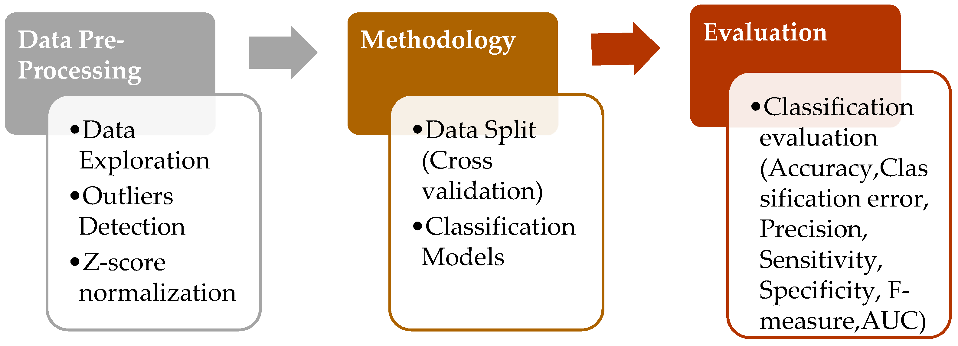
3.8. Data Analysis
Before analyzing the data using the Machine Learning models, preliminary steps were conducted to prepare the data as input to the model. This involved the process of splitting the data into training and testing sets to train the model and validate the model performance. After that, several Machine Learning models were employed to predict Water Quality Classification (WQC) using the identified variables. The methodology used in this study is depicted in Figure 1 below.
3.8.1. Data Partitioning
In data partitioning, the first part of the data was used as training data to parameterize the prediction models, while the last part of the data was used to validate them. Next, the model’s performance was evaluated using the accuracy measures. This study explored the 10-fold cross validation technique to compare and evaluate the candidate models. Cross validation is a method to assess predictive models by dividing the original data into two groups for model training and model validation for ten times and the accuracy of the model is averaged. Typically, the data are divided into two groups for ten times, which are the training dataset and testing dataset in a ratio of 70:30 [6]. The models are then evaluated for predictive accuracy by assessing the difference between the value from the predicted model and the actual value.
3.8.2. Machine Learning Model
The water quality classification (WQC) was assigned to the samples according to their predetermined WQI. This study used 7 classification algorithms for classifying samples into WQC defined earlier. The following classification algorithms were employed in the current study:
- (1)
- K-Nearest Neighbors (KNN)
This K-Nearest Neighbors method classifies samples by discovering the closest neighboring given points and assigns the class of the majority of n neighbors. If there is a draw, different techniques might be used to resolve it. However, KNN is not suggested for a large dataset since all processing occurs during the testing, and it iterates through all training datasets and calculates the nearest neighbor each time [48]. This study utilized the k = 5 configuration for the KNN model.
- (2)
- Support Vector Machine (SVM)
Support Vector Machine is a classifying method based on the theory of statistical learning [33]. SVM uses the structural risk minimization principle to address overfitting problems in Machine Learning by reducing the model’s complexity and fitting the training data successfully. The minimization of risk can enhance the generalization of the SVM model [49]. The estimates of the SVM model are created based on a small sub-set of training data, which is known as support vector. The capability to interpret Support Vector Machine decisions can be improved by recognizing vectors that are chosen as support vectors [50]. SVM maps the initial data in a high-dimension feature space in which an optimal separating plane is created by using a suitable kernel function. For classification, the optimal separating plane is the line that divides the plane into two parts and each class is placed on a different side [10]. Along each part of the separating plane, 2 parallel hyperplanes can be built to separate the training data. Let be the training samples, are the input vector and are the label of class. The hyperplane where is the weights vector, is the input vector and is the bias, is optimal if the margin between the closest training vector and the hyperplane is maximal [51]. The optimal hyperplane can be constructed by solving an optimization problem as follows:
Minimize
subject to
SVM is constructed as a dual optimization problem:
subject to
where is the dual Lagrangian, is the regularization parameter, which is employed to control the trade-off between the margin and the training error.
If is the Lagrange multipliers, optimal hyperplane, can be computed as follows:
Therefore, the non-linear decision function, which is acquired by resolving the dual optimization problem, can be written as follows:
There is a kernel function that allows SVM to make a non-linear classification. The value of equals to , where is the transformation function that changes the input data into higher dimension feature space. Thus, the SVM non-linear decision function can be defined as follows:
where is the inner product kernel function that satisfies the Mercer conditions. There are four commonly used Mercer kernel functions, which are linear kernel, polynomial kernel, Sigmoid and Radial Basis Function kernel [52]. Kernel function expressions are given in Table 4.
This study used a complexity constant, , to set the misclassification tolerance. A high value of can lead to overfitting problems, while a low value may cause overgeneralization. This study used the polynomial kernel since it is suitable for the case in which all training data are normalized [53].
- (3)
- Artificial Neural Network (ANN)
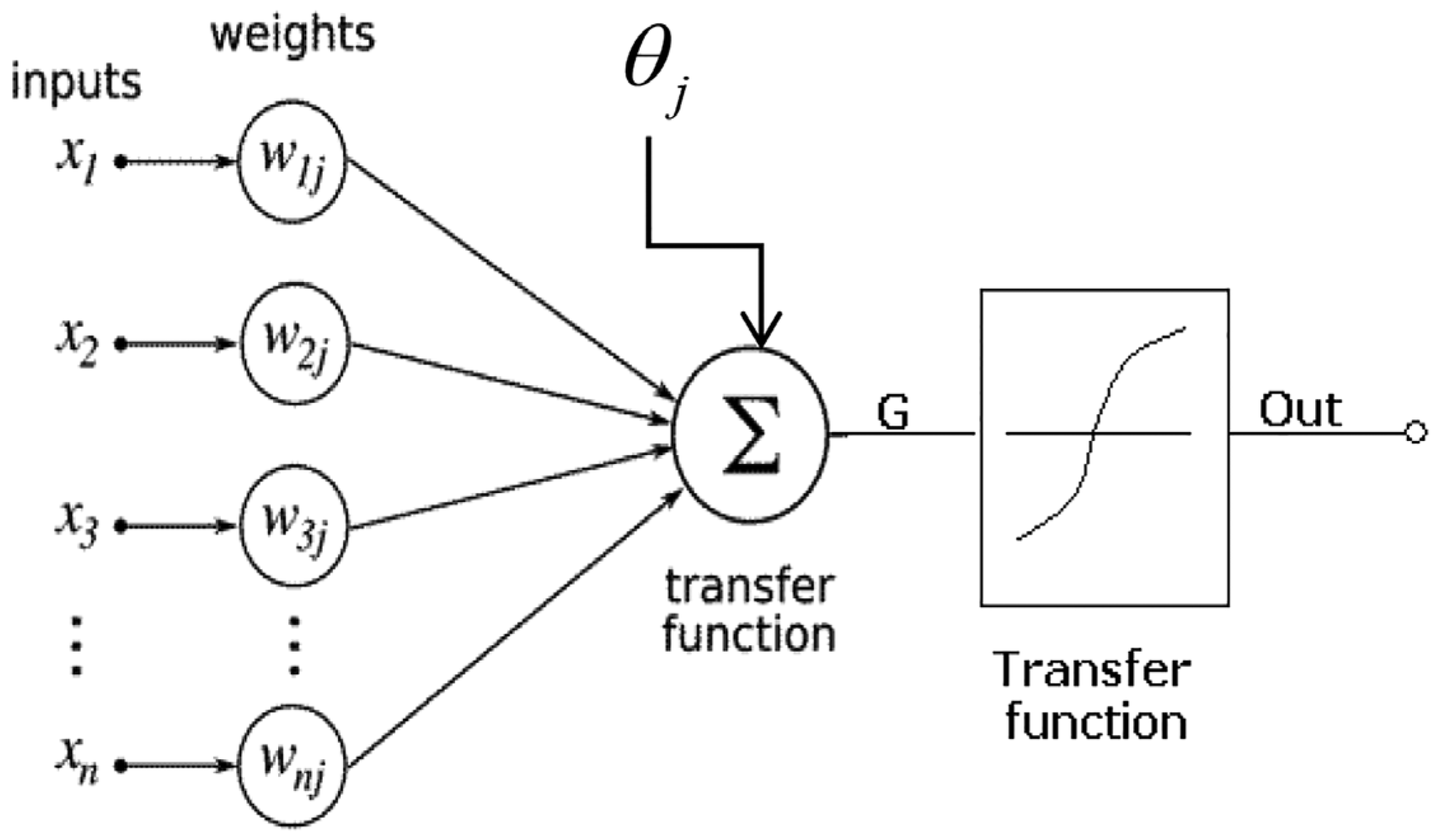
Artificial Neural Network was considered as a benchmark model in this study. It works as a human brain’s nervous system, which comprises interconnected neurons that work together in parallel [54]. It is widely used in many fields because of its advantages, such as self-organizing, self-learning and self-adapting abilities [55]. A neural network comprises four main components, which are inputs, weights, threshold or bias and output. A neural network’s structure is composed of 3 layers, which are the input, middle and output layer. Input variables are entered into the algorithm in the input layer. In the middle layer, the input variables are multiplied by weights before they are summed by a constant value. Then, an activation function is added to the sum of the weighted inputs. Activation functions are needed to transform the input signals into output signals. Recent artificial neural network algorithms employ activation functions that are non-linear. This is because non-linear activation functions allow backpropagation and multi-layer neurons stacking to produce a complex mapping between input and output networks, which are needed to study a complex dataset. The most popular activation functions are Gaussian, Sigmoid and Tansig [56]. In the output layer, the prediction is obtained from the parallel computation in the middle layer. Mathematical neural operations are shown in Figure 2.
The mathematical formula of neuron computation is given below:
where is the symbol for denotation of mathematical formula of neuron, is the weights, is the input variables and is the biases.
In a feed-forward neural network, input data propagate in a forward direction through the network, which means that every hidden layer receives the input from the input layer and produces the final output. As a result, the final output depends on input data, weight parameters and the choice of activation function [57]. Gradient descent optimization is used to adjust the weights within the neural network framework to minimize the error between the expected output and actual output. The selection of weight is based upon the performance measurement, such as mean-squared error [30]. Multi-layer Perceptron (MLP) is a completely connected feed-forward artificial neural network that contains at least a hidden layer [58]. Although MLP can have any number of hidden layers, generally, one hidden layer is sufficient. This is because the number of hidden layers has a significant effect on MLP performance. The training process will take a longer time and overfitting problems may occur if there are too many layers. This study used the default hidden layer that consisted of one hidden layer with the Sigmoid activation function and a size equal to (number of attributes + number of classes)/2 + 1. This study used the default value of 200 for training cycles, a learning rate of 0.01 and a momentum of 0.8.
- (4)
- Decision Tree
The decision tree (DT) is an explicit, simple algorithm that makes decisions founded on the values from all pertinent input parameters. DT uses entropy for selecting the root variable and, depending on it, reviews the values of the other parameters. DT obtained all decisions of the parameters arranged in a top-down tree and plans the decision according to different values from different parameters [59]. Decision tree models are frequently found in previous studies to perform well on imbalanced data. However, decision-tree-based ensemble models, including Random Forest (RF) and Gradient Boosting (GB), almost always outperform the single decision tree. The advantages of decision-tree-based model are the fact that they are not sensitive to missing values, are able to manage both regular attributes and data, and are highly efficient. Compared to other ML models, decision-tree-based models are more favorable for short-term predictions and may have a quicker calculation speed [14].
- (5)
- Naïve Bayes
The Bayes approach employs probability statistics knowledge to classify the data and estimate the outcome. The Bayes model uses prior and posterior probabilities in order to prevent overfitting problems and bias from using only sample information. A classification technique that uses the Bayes theorem and the independent conditions assumption is known as Naïve Bayes (NB). When the target value is specified, the attributes are meant to be conditionally independent from each other. This technique makes the complexity of the Bayes model much simpler. The probability that Event would occur given that Event occurred is different than the probability that Event would occur given that Event occurred as indicated in the equation below:
Assuming that are the event vectors and is the dataset class, the Bayes formula may be described as shown below:
where the is a prior probability that represents the event vectors and is the dataset class prior probability. This study used default values for this algorithm.
- (6)
- Random Forest (RF)
Random forest is one of the classification models that employs multiple base classifiers, typically decision trees, on a given subset of data independently and makes decisions based on all models [9]. It uses feature randomness and bagging when building each individual decision tree to produce an independent forest of trees. Random forest is a method of calculating the mean of several deep decision trees formed in different parts of the same training set, with the aim of reducing the variance. The prediction by this committee is more accurate than that of any individual tree and is robust against overfitting. Bagging, also known as Bootstrap Aggregating, is used to decrease the variance in the prediction by generating additional data for training from the dataset using combinations with repetitions to produce multi-sets of the original data. RF provides all the benefits of a decision tree with the added efficiency of using more than one model [35]. In standard decision trees, each node is split using the best split among all parameters. However, in RF, each node is split using the best split among a subset of parameters that is randomly chosen [60]. RF has 2 parameters, which are the number of samples in the random subset (maximal depth) and the number of trees in the forest to be included [61]. This parameter can be selected by increasing or decreasing the number of trees in run after run, until the accuracy starts to show no improvement. This study used the default values with a number of trees of 100 and a maximal depth of 10. The Random Forest algorithm works as follows:
- Create ntree bootstrap sub-samples of the original dataset with replacement.
- For each bootstrap samples, train a decision tree model.
- Predict the new data by aggregating the prediction of the ntree models (majority votes for classification).
- (7)
- Gradient Boosting (GB)
Gradient boosting is a Machine Learning technique that trains multiple weak classifiers, typically decision trees, to create a robust classifier for the regression and classification problems. It assembles the model in a stage-wise way similar to the other boosting techniques and it generalizes them by optimizing a suitable cost function. In the GB algorithm, incorrectly classified cases for a step are given increased weight during the next step. The advantages of GB are that it has exceptional accuracy in predicting and fast process [36]. This technique is quite similar to Adaptive Boosting (AdaBoost) but the drawback of AdaBoost is the efficiency of the technique, which is highly affected by outliers and easily overwhelmed by noisy data [62]. This study used the default values for gradient boosting with a maximal depth of 5, a number of trees of 50 and a learning rate of 0.1.
3.9. Imbalanced Data Issue
One of the main challenges of Machine Learning is the processing of imbalance data for the classification [63]. An imbalanced dataset is a situation in which the occurrence of one outcome from two possible outcomes is very rare [64]. The data are unevenly distributed in classes and certain classes have large samples (majority classes), while some have a few samples (minority classes). In this kind of dataset, not even a single sample of the minority class is classified correctly, and accuracy can reach up to 99%. It means that, when imbalanced data occur, classifiers have a tendency to make a biased model that has a poorer predictive accuracy over the minority class. Moreover, the gap between sensitivity and specificity may become large, especially in traditional classifiers [65]. Therefore, the classification of imbalanced data becomes a highly explored issue because it creates a bias in the performance of traditional classifiers. They consider the error rate, but not the distribution of data, and the minority class samples are removed from the overall classification result [66]. The modification of the existing classifier to accommodate imbalanced data, such as using ensemble methods, has been proven to be successful. Ensemble models, such as Gradient Boosting and Random Forest, can improve the sensitivity and specificity of the prediction.
3.10. Accuracy Measures
The target variable used in this study was the water quality classification. Since there was no observation for the polluted class as classified according to the WQI formulation, this study used a binary target to predict WQC for the 2 classes of slightly polluted and clean. Thus, we considered the 2 × 2 confusion matrix, as given in Table 5, to evaluate model performance. The classifiers were basically assessed by a confusion matrix in the Machine Learning study. The confusion matrix is a tabular way to illustrate the performance of the predictive model. Each entry in the confusion matrix indicates the number of correct or false classifications made by the model. For binary class problem, the confusion matrix is a square of 2 × 2, where the row is the class label real value, while the column signifies the classifier prediction. In an imbalanced data situation, the instances from the minority class are labelled as positive, while the instances from majority class are labelled as negative.
This study used 8 different measures to evaluate the accuracy of classifiers. The measurements are listed below:
- (1)
- Balanced Accuracy
Balanced accuracy is a good measure to use when data are out of balance. It takes into account both positive and negative outcome classes and makes no mistake with imbalanced data [67]. Since the number of clean classes is significantly higher than the slightly polluted class in the dataset, this study calculated the balanced accuracy to cater for the imbalanced data. The formula for balanced accuracy is shown below:
Balanced Accuracy = (Sensitivity + Specificity)/2
In other words, balanced accuracy is the mean for sensitivity and specificity. If the classifier works equally well on both classes, it is reduced to conventional accuracy. However, the balanced accuracy will decrease if the classifier only benefits from the prediction regarding the majority class [67]. For classification problems, the best score for accuracy is 100%. However, this score is impossible to achieve since all predictive models have prediction errors. The model performance accuracy falls between the baseline and the best possible performance score [68].
- (2)
- Accuracy
Accuracy is the most common measure used for classifier assessment. It assesses the overall efficiency of the algorithm by estimating the likelihood of the actual value of the class label. Accuracy is calculated using the equation below:
where TP is true positive, TN is true negative, FN is false negative and TN is true negative [69].
Accuracy = (TP + TN)/(TP + FP + FN + TN)
- (3)
- Classification Error
Classification error is an estimate of the probability of misclassification based on model prediction [70]. The classification error is defined as follows:
Classification error = 1 − accuracy
- (4)
- Precision
Precision, or positive predictive value (PPV), is the proportion of correctly identified positive outcomes over all positive predictions. Precision can be defined as:
where TP is true positive and FP is false positive [71].
Precision = TP/(TP + FP)
- (5)
- Specificity
Specificity is the measure of true negative outcomes that are correctly predicted. Specificity is described as follows:
where TN is true negative and FP is false positive.
Specificity = TN/(TN + FP)
- (6)
- Sensitivity
Sensitivity, or recall, calculates the percentage of true positive outcomes that are correctly predicted. Sensitivity is defined as follows:
where TP is true positive and FN is false negative [71].
Sensitivity = TP/(TP + FN)
- (7)
- F-measure
The F-measure is the harmonic mean of accuracy and recall that better reflects the overall measurement of accuracy. F-measure varies between 0 and 1. The accuracy is better if the score is higher [61,63]. The f-measure can be calculated as follows:
F-measure = (2xPrecision × Recall)/(Precision + Recall)
- (8)
- Area Under the Curve (AUC)
AUC is a vital evaluation metric to examine the performance of any classification model. AUC represents the separability measurement. From AUC, the capability of the model to distinguish between classes can be identified. The model is better in predicting if the AUC value is high. A model with an AUC value approximate of 1 indicates that the model is excellent and has a good separability measurement, while a model with an AUC value close to 0 indicates that the model is poor and has the worst separability measurement. In other words, the model predicts that the positive class is the negative class and the negative class is the positive class [72]. When the AUC is 0.8, this means that there is 80% chance that the model will be able to differentiate between the negative and positive class. When the AUC is around 0.5, this indicates the model does not have the capacity to discriminate between the negative and positive class. The formula for AUC is as follows:
AUC = (1 + TPR − FPR)/2
4. Results
4.1. Descriptive Statistics
There were 658 observations in the water quality dataset coming from 8 stations along the Kelantan River from the year 2005 to 2020. Table 6 shows the minimum, maximum, mean and standard deviation values for the variables Dissolved Oxygen (DO), Biochemical Oxygen Demand (BOD), Chemical Oxygen Demand (COD), Total Suspended Solid (TSS), pH, NH3N, temperature, conductivity, salinity, turbidity, nitrogen, phosphorus and E. coli, after standardization using z-score normalization. Based on Table 6, the mean values for DO, BOD, COD, TSS, pH, NH3N, temperature, conductivity, salinity, turbidity, nitrogen, phosphorus and E. coli were 0.0020, −0.0315, −0.0380, −0.0687, −0.0074, −0.0664, −0.0025, −0.0784, −0.0784, −0.0718, −0.0547, −0.0579 and −0.0548, respectively, while the standard deviations for all the variables were 1.0032, 0.9393, 0.8485, 0.7188, 0.9979, 0.4260, 0.9984, 0.1984, 0.1840, 0.7794, 0.6158, 0.4193, 0.2747, respectively.
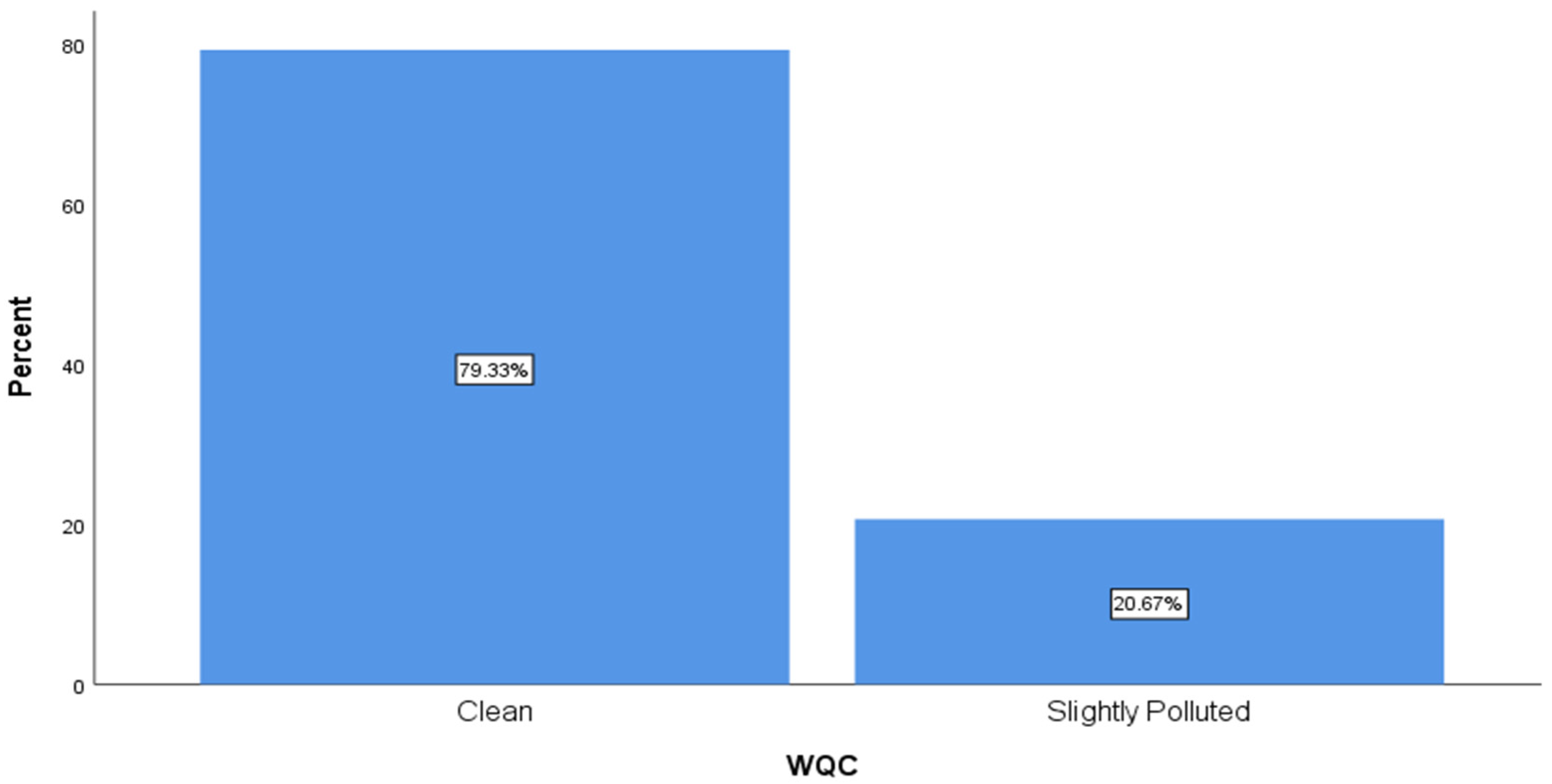
Meanwhile, regarding the target variable of this study, which was Water Quality Class (WQC), 79.33% of the data belonged to the clean class and 20.67% of the data belonged to the slightly polluted class, as shown in Figure 3.
4.2. Machine Learning Models Performance Comparison
In this section, the results of the Water Quality Classification (WQC) prediction using seven Machine Learning models are presented. These classification algorithms used 13 input parameters, which were Dissolved Oxygen (DO), Biochemical Oxygen Demand (BOD), Chemical Oxygen Demand (COD), Ammoniacal Nitrogen (NH3-N), Total Suspended Solid (TSS), pH, E. coli, temperature, turbidity, conductivity, salinity, nitrogen and phosphorus. Based on the results, Gradient Boosting (GB) performed the best in comparison to the other algorithms in terms of balanced accuracy, accuracy, classification error, precision, specificity and f-measure. It had the highest balanced accuracy of 89.36%, accuracy of 94.90%, precision of 94.12%, specificity of 98.72%, f-measure of 86.49% and an AUC value of 0.9811, with the lowest classification error. This was followed by Random Forest (RF) with a slightly lower accuracy, precision, specificity and f-measure, the same sensitivity value, but higher AUC value compared to GB. This study also found that Decision Tree performed the worst in predicting WQC with a balanced accuracy of 80.19%, accuracy of 86.22%, classification error of 13.78%, sensitivity of 70% and f-measure of 67.47%, as shown in Table 7. However, in terms of sensitivity, the ANN model had the highest value compared to the other models. This high value might be due to the fact that ANN sometimes has unexplained network behaviour [73].
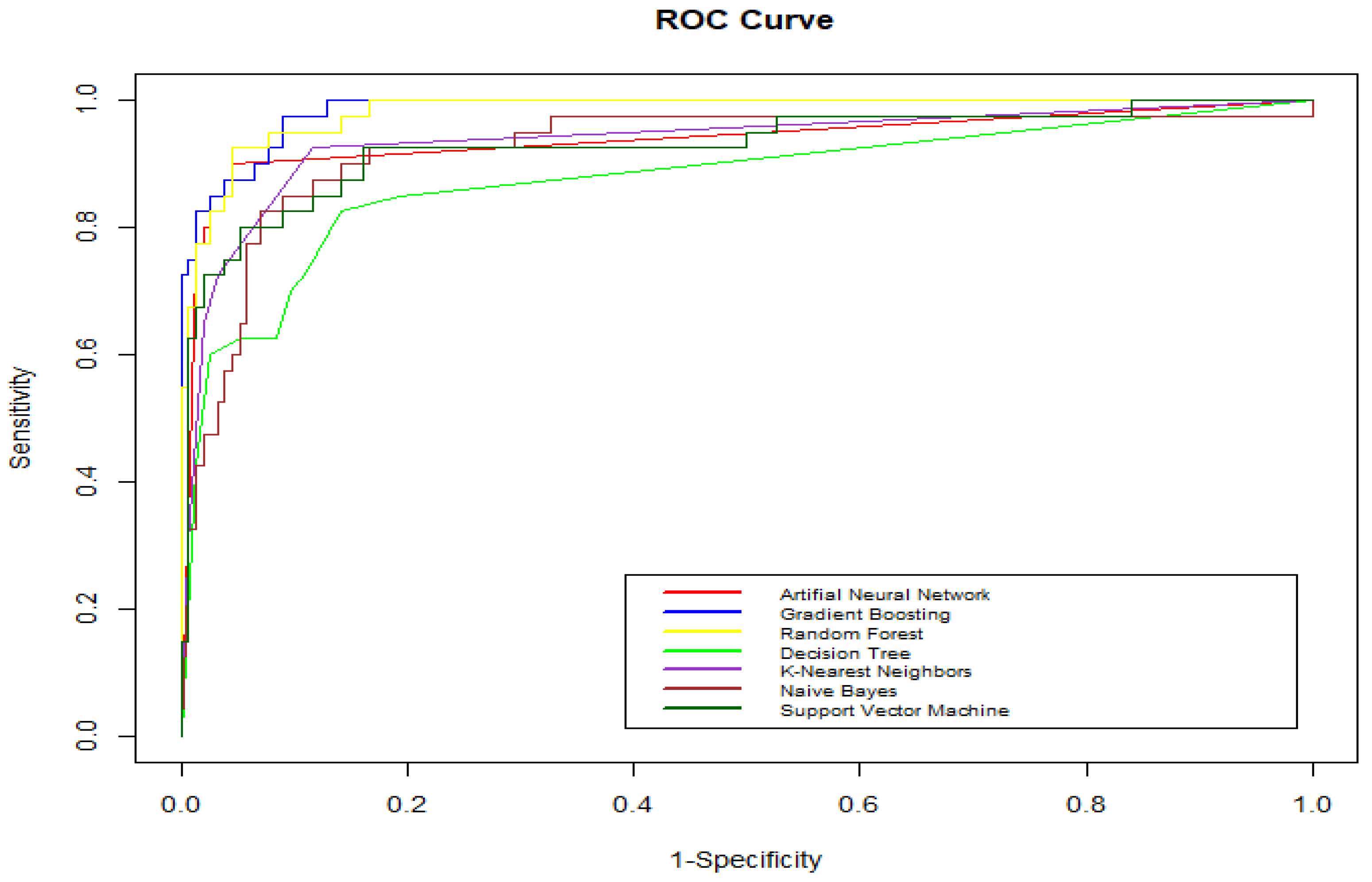
4.3. ROC Comparison
This study used ROC charts to compare the performance of all seven Machine Learning algorithms. ROC chart is a graph showing the false positive rate (1-specificity) in the horizontal axis and the true positive rate (sensitivity) in the vertical axis. Ideally, the curve climbed rapidly up to the top left, which means the model correctly predicted the cases. Based on the ROC charts shown in Figure 4, Gradient Boosting is the best model compared to the other models because the curve is the closest to the top left corner of the plot.
4.4. Gradient Bossting Model for WQC
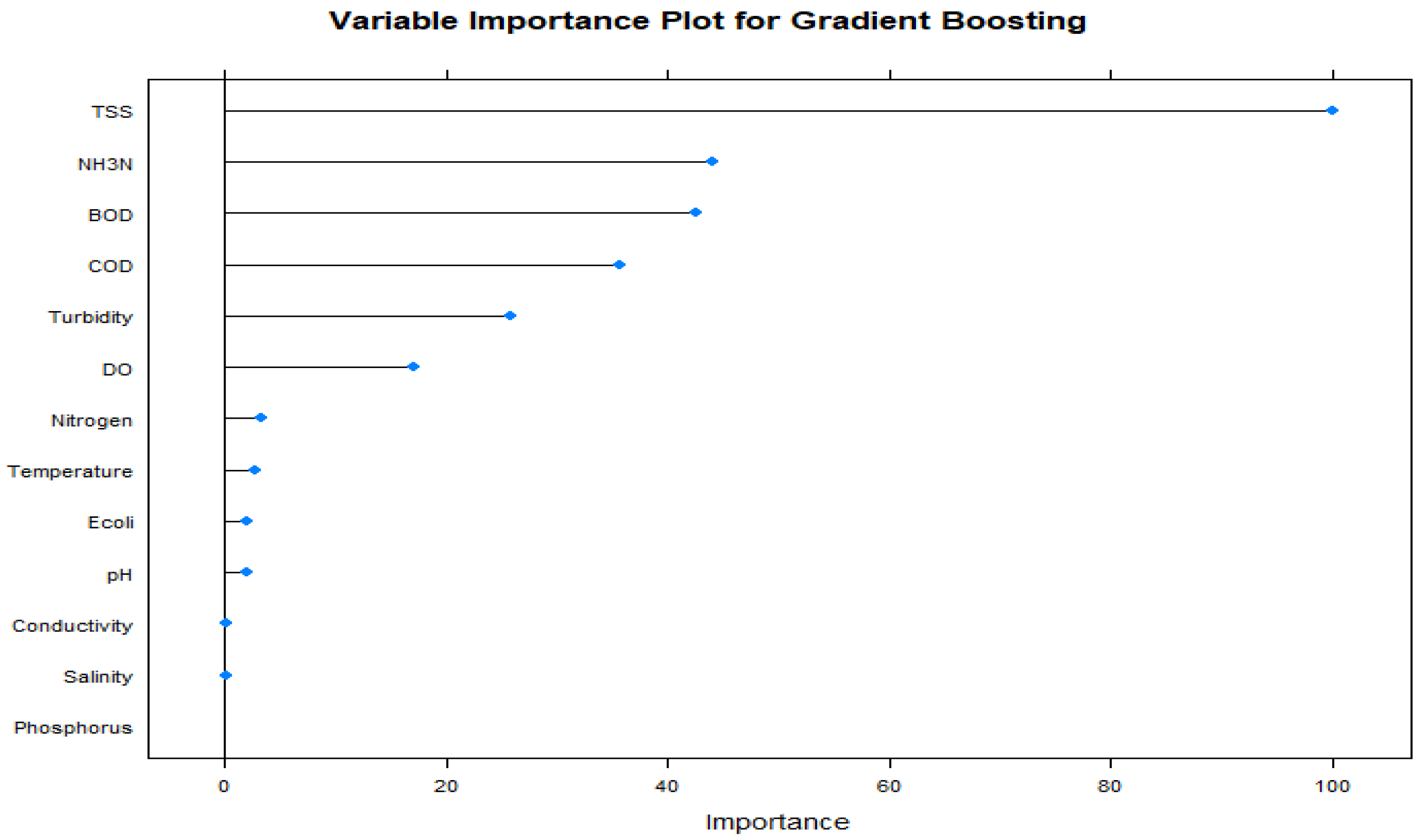
The predictor importance for the Gradient Boosting model (Figure 5) shows that Total Suspended Solid (TSS) is the most important variable for the Gradient Boosting (GB) model to predict WQC, followed by Ammoniacal Nitrogen (NH3N), Biochemical Oxygen Demand (BOD), Chemical Oxygen Demand (COD), Turbidity and Dissolved Oxygen (DO) (Figure 4). This model used the variance-based method to compute the importance of the predictor.
5. Discussion
Based on the results, decision-tree-based ensemble models, such as Random Forest and Gradient Boosting, always outperform the single decision tree methods since they combine multiple decision trees and use the average of the outputs to produce a better model. Gradient Boosting assembles the model in a stage-wise way similar to the other boosting techniques and it generalizes them by optimizing a suitable cost function. Boosting learns homogeneous weak learners sequentially in a very adaptative way (a base model depends on the previous ones) and combines them by following a deterministic strategy. Meanwhile, Random Forest uses bagging and feature randomness when building each individual tree to try to create an uncorrelated forest of trees whose prediction by committee is more accurate than that of individual trees. Bagging, also known as Bootstrap Aggregating, is the application of the bootstrap procedure to a high-variance Machine Learning algorithm to decrease the variance in the prediction by generating additional data for training from a dataset using combinations with repetitions to produce multi-sets of the original data. This study also found that Decision Tree (DT) performed the worst in the prediction of WQC. Although the ANN model did not perform very well, it had the highest sensitivity value compared to the other models. This might be due to the fact that ANN sometimes has unexplained network behaviour [73]. When ANN produces a probing solution, it provides no guidance on why and how, which decreases the confidence in the network.
6. Conclusions
This study explored a series of Machine Learning models for predicting water quality classification (WQC), which is a distinguishing class defined on the basis of the water quality index. The proposed methodology employed 13 input parameters of water quality and 7 Machine Learning models, which included K-Nearest Neighbour, Artificial Neural Network, Decision Tree, Naïve Bayes, Support Vector Machine, Random Forest and Gradient Boosting. Based on the analysis, Gradient Boosting with a learning rate of 0.1 predicted the WQC most efficiently compared to all seven employed algorithms. It had the highest balanced accuracy, accuracy, precision, specificity and f-measure, with the lowest classification error. These findings are supported by the result of the ROC chart for Gradient Boosting. The second best model was Random Forest and the worst model was Decision Tree, which had the lowest performance measures for all metrics. Therefore, based on accurate water quality prediction, the results could help to improve water quality continuously as well as the National Environmental Policy regarding water resources, and to conserve the diversity and liveliness of the river. For future works, this study suggests that the issue of imbalanced data in the water quality data should be highlighted since it affects the prediction accuracy.
Author Contributions
Conceptualization, N.H.A.M. and W.F.W.Y.; methodology, N.H.A.M. and W.F.W.Y.; software, N.H.A.M.; validation, W.F.W.Y., S.A.M.N. and N.S.; formal analysis, N.H.A.M.; investigation, N.H.A.M.; resources, N.H.A.M. and W.F.W.Y.; data curation, N.H.A.M.; writing—original draft preparation, N.H.A.M.; writing—review and editing, W.F.W.Y. and S.A.M.N.; visualization, N.H.A.M.; supervision, W.F.W.Y., S.A.M.N. and N.S.; project administration, N.H.A.M. and W.F.W.Y.; funding acquisition, W.F.W.Y. All authors have read and agreed to the published version of the manuscript.
Funding
The authors would like to thank Universiti Teknologi MARA for funding this research under Geran Insentif Penyeliaan (600-RMC/GIP 5/3 (065/2021)).
Data Availability Statement
Restrictions apply to the availability of these data. Data was obtained from Department of Environment Malaysia (DOE) and are available with the permission of DOE.
Acknowledgments
The authors would like to thank the reviewers for their helpful and constructive comments and suggestions that greatly contributed to improve the final version of this paper.
Conflicts of Interest
The authors declare no conflict of interest.
References
- Ling, J.K.B. Water Quality Study and Its Relationship with High Tide and Low Tide at Kuantan River. Bachelor’s Thesis, Universiti Malaysia Pahang, Gambang, Malaysia, 2010. Available online: http://umpir.ump.edu.my/id/eprint/2449/1/JACKY_LING_KUO_BAO.PDF (accessed on 22 February 2022).
- Xu, J.; Gao, X.; Yang, Z.; Xu, T. Trend and Attribution Analysis of Runoff Changes in the Weihe River Basin in the Last 50 Years. Water 2022, 14, 47. [Google Scholar] [CrossRef]
- Wahab, M.A.A.; Jamadon, N.K.; Mohmood, A.; Syahir, A. River Pollution Relationship to the National Health Indicated by Under-Five Child Mortality Rate: A Case Study in Malaysia. Bioremediat. Sci. Technol. Res. 2015, 3, 20–25. [Google Scholar]
- Zainudin, Z. Benchmarking river water quality in Malaysia. Jurutera 2010, 12, 15. [Google Scholar]
- Abbasi, T.; Abbasi, S.A. Water Quality Indices; Elsevier: Amsterdam, The Netherlands, 2012. [Google Scholar]
- Bui, D.T.; Khosravi, K.; Tiefenbacher, J.; Nguyen, H.; Kazakis, N. Improving prediction of water quality indices using novel hybrid machine-learning algorithms. Sci. Total Environ. 2020, 721, 137612. [Google Scholar] [CrossRef]
- Malek, N.H.A.; Yaacob, W.F.W.; Nasir, S.A.M.; Shaadan, N. The Effect of Chemical Parameters on Water Quality Index in Machine Learning Studies: A Meta-Analysis. J. Phys. Conf. Ser. 2021, 2084, 12007. [Google Scholar] [CrossRef]
- Sharafati, A.; Asadollah, S.B.H.S.; Hosseinzadeh, M. The potential of new ensemble machine learning models for effluent quality parameters prediction and related uncertainty. Process Saf. Environ. Prot. 2020, 140, 68–78. [Google Scholar] [CrossRef]
- Ahmed, U.; Mumtaz, R.; Anwar, H.; Shah, A.A.; Irfan, R.; García-Nieto, J. Efficient water quality prediction using supervised machine learning. Water 2019, 11, 2210. [Google Scholar] [CrossRef] [Green Version]
- Xu, T.; Coco, G.; Neale, M. A predictive model of recreational water quality based on adaptive synthetic sampling algorithms and machine learning. Water Res. 2020, 177, 115788. [Google Scholar] [CrossRef]
- Gakii, C.; Jepkoech, J. A Classification Model for Water Quality analysis Using Decision Tree. Eur. J. Comput. Sci. Inf. Technol. 2019, 7, 1–8. [Google Scholar]
- Jeihouni, M.; Toomanian, A.; Mansourian, A. Decision tree-based data mining and rule induction for identifying high quality groundwater zones to water supply management: A novel hybrid use of data mining and GIS. Water Resour. Manag. 2020, 34, 139–154. [Google Scholar] [CrossRef] [Green Version]
- Vijay, S.; Kamaraj, K. Ground Water Quality Prediction using Machine Learning Algorithms in R. Int. J. Res. Anal. Rev. 2019, 6, 743–749. [Google Scholar]
- Lu, H.; Ma, X. Hybrid decision tree-based machine learning models for short-term water quality prediction. Chemosphere 2020, 249, 126169. [Google Scholar] [CrossRef] [PubMed]
- Abyaneh, H.Z. Evaluation of multivariate linear regression and artificial neural networks in prediction of water quality parameters. J. Environ. Health Sci. Eng. 2014, 12, 40. [Google Scholar] [CrossRef] [PubMed] [Green Version]
- Alias, S.W.A.N. Ecosystem Health Assessment of Sungai Pengkalan Chepa Basin: Water Quality and Heavy Metal Analysis. Sains Malays. 2020, 49, 1787–1798. [Google Scholar]
- Al-Badaii, F.; Shuhaimi-Othman, M.; Gasim, M.B. Water quality assessment of the Semenyih river, Selangor, Malaysia. J. Chem. 2013, 2013, 871056. [Google Scholar] [CrossRef] [Green Version]
- Asadollah, S.B.H.S.; Sharafati, A.; Motta, D.; Yaseen, Z.M. River water quality index prediction and uncertainty analysis: A comparative study of machine learning models. J. Environ. Chem. Eng. 2021, 9, 104599. [Google Scholar] [CrossRef]
- Chen, K.; Chen, H.; Zhou, C.; Huang, Y.; Qi, X.; Shen, R.; Liu, F.; Zuo, M.; Zou, X.; Wang, J. Comparative analysis of surface water quality prediction performance and identification of key water parameters using different machine learning models based on big data. Water Res. 2020, 171, 115454. [Google Scholar] [CrossRef]
- Lerios, J.L.; Villarica, M.V. Pattern Extraction of Water Quality Prediction Using Machine Learning Algorithms of Water Reservoir. Int. J. Mech. Eng. Robot. Res. 2019, 8, 992–997. [Google Scholar] [CrossRef]
- Sengorur, B.; Koklu, R.; Ates, A. Water quality assessment using artificial intelligence techniques: SOM and ANN—A case study of Melen River Turkey. Water Qual. Expo. Health 2015, 7, 469–490. [Google Scholar] [CrossRef]
- Aradhana, G.; Singh, N.B. Comparison of Artificial Neural Network algorithm for water quality prediction of River Ganga. Environ. Res. J. 2014, 8, 55–63. [Google Scholar]
- Ahmad, Z.; Rahim, N.A.; Bahadori, A.; Zhang, J. Improving water quality index prediction in Perak River basin Malaysia through a combination of multiple neural networks. Int. J. River Basin Manag. 2017, 15, 79–87. [Google Scholar] [CrossRef] [Green Version]
- Gazzaz, N.M.; Yusoff, M.K.; Aris, A.Z.; Juahir, H.; Ramli, M.F. Artificial neural network modeling of the water quality index for Kinta River (Malaysia) using water quality variables as predictors. Mar. Pollut. Bull. 2012, 64, 2409–2420. [Google Scholar] [CrossRef] [PubMed]
- Hameed, M.; Sharqi, S.S.; Yaseen, Z.M.; Afan, H.A.; Hussain, A.; Elshafie, A. Application of artificial intelligence (AI) techniques in water quality index prediction: A case study in tropical region, Malaysia. Neural Comput. Appl. 2017, 28, 893–905. [Google Scholar] [CrossRef]
- Babbar, R.; Babbar, S. Predicting river water quality index using data mining techniques. Environ. Earth Sci. 2017, 76, 1–15. [Google Scholar] [CrossRef]
- Liu, M.; Lu, J. Support vector machine—An alternative to artificial neuron network for water quality forecasting in an agricultural nonpoint source polluted river? Environ. Sci. Pollut. Res. 2014, 21, 11036–11053. [Google Scholar] [CrossRef]
- Mohammadpour, R.; Shaharuddin, S.; Chang, C.K.; Zakaria, N.A.; Ab Ghani, A.; Chan, N.W. Prediction of water quality index in constructed wetlands using support vector machine. Environ. Sci. Pollut. Res. 2015, 22, 6208–6219. [Google Scholar] [CrossRef]
- Sattari, M.T.; Joudi, A.R.; Kusiak, A. Estimation of Water Quality Parameters with Data—Driven Model. J.-Am. Water Work. Assoc. 2016, 108, E232–E239. [Google Scholar] [CrossRef] [Green Version]
- Muhammad, S.Y.; Makhtar, M.; Rozaimee, A.; Aziz, A.A.; Jamal, A.A. Classification model for water quality using machine learning techniques. Int. J. Softw. Eng. Its Appl. 2015, 9, 45–52. [Google Scholar] [CrossRef]
- Naghibi, S.A.; Hashemi, H.; Berndtsson, R.; Lee, S. Application of extreme gradient boosting and parallel random forest algorithms for assessing groundwater spring potential using DEM-derived factors. J. Hydrol. 2020, 589, 125197. [Google Scholar] [CrossRef]
- Khosravi, K.; Mao, L.; Kisi, O.; Yaseen, Z.M.; Shahid, S. Quantifying hourly suspended sediment load using data mining models: Case study of a glacierized Andean catchment in Chile. J. Hydrol. 2018, 567, 165–179. [Google Scholar] [CrossRef]
- Vapnik, V. The Nature of Statistical Learning Theory; Springer: New York, NY, USA, 1995. [Google Scholar]
- Ahmed, S.; Mahbub, A.; Rayhan, F.; Jani, R.; Shatabda, S.; Farid, D.M. Hybrid methods for class imbalance learning employing bagging with sampling techniques. In Proceedings of the Computational Systems and Information Technology for Sustainable Solution (CSITSS), Bengaluru, India, 21–23 December 2017; pp. 1–5. [Google Scholar]
- Liaw, A.; Wiener, M. Classification and regression by randomForest. R News 2002, 2, 18–22. [Google Scholar]
- Prakash, R.; Tharun, V.P.; Devi, S.R. A Comparative Study of Various Classification Techniques to Determine Water Quality. In Proceedings of the Inventive Communication and Computational Technologies (ICICCT), Coimbatore, India, 20–21 April 2018; pp. 1501–1506. [Google Scholar]
- Sekitar, M.J.A. Pengelasan Indeks Kualiti air sungai. 2018; 7–8. [Google Scholar]
- Aldhyani, T.H.H.; Al-Yaari, M.; Alkahtani, H.; Maashi, M. Water Quality Prediction Using Artificial Intelligence Algorithms. Appl. Bionics Biomech. 2020, 2020, 6659314. [Google Scholar] [CrossRef]
- Jayalakshmi, T.; Santhakumaran, A. Statistical normalization and back propagation for classification. Int. J. Comput. Theory Eng. 2011, 3, 1793–8201. [Google Scholar]
- Nnamoko, N.; Korkontzelos, I. Efficient treatment of outliers and class imbalance for diabetes prediction. Artif. Intell. Med. 2020, 104, 101815. [Google Scholar] [CrossRef]
- Robinson, R.B.; Cox, C.D.; Odom, K. Identifying outliers in correlated water quality data. J. Environ. Eng. 2005, 131, 651–657. [Google Scholar] [CrossRef]
- Kwak, S.K.; Kim, J.H. Statistical data preparation: Management of missing values and outliers. Korean J. Anesthesiol. 2017, 70, 407. [Google Scholar] [CrossRef]
- Hair, J.F.; Anderson, R.E.; Babin, B.J.; Black, W.C. Multivariate Data Analysis: A Global Perspective; Pearson Education: London, UK, 2010; Volume 7. [Google Scholar]
- Ghapor, A.A.; Zubairi, Y.Z.; Imon, A.H.M.R. Missing value estimation methods for data in linear functional relationship model. Sains Malays. 2017, 46, 317–326. [Google Scholar] [CrossRef]
- Little, R.J.A.; Rubin, D.B. Statistical Analysis with Missing Data; John Wiley & Sons: Hoboken, NJ, USA, 2019; Volume 793. [Google Scholar]
- Dempster, A.P.; Laird, N.M.; Rubin, D.B. Maximum likelihood from incomplete data via the EM algorithm. J. R. Stat. Soc. Ser. B (Methodol.) 1977, 39, 1–22. [Google Scholar]
- Musil, C.M.; Warner, C.B.; Yobas, P.K.; Jones, S.L. A comparison of imputation techniques for handling missing data. West. J. Nurs. Res. 2002, 24, 815–829. [Google Scholar] [CrossRef] [PubMed]
- Beyer, K.; Goldstein, J.; Ramakrishnan, R.; Shaft, U. When is “nearest neighbor” meaningful? In Proceedings of the Database Theory, Berlin/Heidelberg, Germany, 10–12 January 1999; pp. 217–235. [Google Scholar]
- Behzad, M.; Asghari, K.; Eazi, M.; Palhang, M. Generalization performance of support vector machines and neural networks in runoff modeling. Expert Syst. Appl. 2009, 36, 7624–7629. [Google Scholar] [CrossRef]
- Nalepa, J.; Kawulok, M. Selecting training sets for support vector machines: A review. Artif. Intell. Rev. 2019, 52, 857–900. [Google Scholar] [CrossRef] [Green Version]
- Kecman, V. Support Vector Machines—An Introduction; Springer: Berlin/Heidelberg, Germany, 2005; pp. 1–47. [Google Scholar]
- Vapnik, V.; Chapelle, O. Bounds on error expectation for support vector machines. Neural Comput. 2000, 12, 2013–2036. [Google Scholar] [CrossRef] [Green Version]
- Bhavsar, H.; Panchal, M.H. A review on support vector machine for data classification. Int. J. Adv. Res. Comput. Eng. Technol. (IJARCET) 2012, 1, 185–189. [Google Scholar]
- Zahiri, A.; Dehghani, A.A.; Azamathulla, H.M. Application of Gene-Expression Programming in Hydraulic Engineering; Springer: Berlin/Heidelberg, Germany, 2015; pp. 71–97. [Google Scholar]
- Anctil, F.; Perrin, C.; Andréassian, V. Impact of the length of observed records on the performance of ANN and of conceptual parsimonious rainfall-runoff forecasting models. Environ. Model. Softw. 2004, 19, 357–368. [Google Scholar] [CrossRef]
- Haghiabi, A.H.; Nasrolahi, A.H.; Parsaie, A. Water quality prediction using machine learning methods. Water Qual. Res. J. 2018, 53, 3–13. [Google Scholar] [CrossRef]
- Witten, I.H.; Frank, E.; Hall, M.A.; Pal, C.J. Practical machine learning tools and techniques. Morgan Kaufmann 2005, 2, 4. [Google Scholar]
- Johnson, J.M.; Khoshgoftaar, T.M. Survey on deep learning with class imbalance. J. Big Data 2019, 6, 27. [Google Scholar] [CrossRef]
- Quinlan, J.R. Decision trees and decision-making. IEEE Trans. Syst. Man Cybern. 1990, 20, 339–346. [Google Scholar] [CrossRef]
- Breiman, L. Random forests. Mach. Learn. 2001, 45, 5–32. [Google Scholar] [CrossRef] [Green Version]
- Dietterich, T.G. An experimental comparison of three methods for constructing ensembles of decision trees: Bagging, boosting, and randomization. Mach. Learn. 2000, 40, 139–157. [Google Scholar] [CrossRef]
- Friedman, J.H. Stochastic gradient boosting. Comput. Stat. Data Anal. 2002, 38, 367–378. [Google Scholar] [CrossRef]
- He, H.; Garcia, E.A. Learning from imbalanced data. IEEE Trans. Knowl. Data Eng. 2009, 21, 1263–1284. [Google Scholar]
- Tyagi, S.; Mittal, S. Sampling Approaches for Imbalanced Data Classification Problem in Machine Learning; Springer: Berlin/Heidelberg, Germany, 2020; pp. 209–221. [Google Scholar]
- Banerjee, P.; Dehnbostel, F.O.; Preissner, R. Prediction Is a Balancing Act: Importance of Sampling Methods to Balance Sensitivity and Specificity of Predictive Models Based on Imbalanced Chemical Data Sets. Front. Chem. 2018, 6. [Google Scholar] [CrossRef]
- Patel, H.; Singh Rajput, D.; Thippa Reddy, G.; Iwendi, C.; Kashif Bashir, A.; Jo, O. A review on classification of imbalanced data for wireless sensor networks. Int. J. Distrib. Sens. Netw. 2020, 16, 1550147720916404. [Google Scholar] [CrossRef]
- Brodersen, K.H.; Ong, C.S.; Stephan, K.E.; Buhmann, J.M. The balanced accuracy and its posterior distribution. In Proceedings of the Pattern Recognition, Istanbul, Turkey, 23–26 August 2010; pp. 3121–3124. [Google Scholar]
- Valverde-Albacete, F.J.; Peláez-Moreno, C. 100% classification accuracy considered harmful: The normalized information transfer factor explains the accuracy paradox. PLoS ONE 2014, 9, e84217. [Google Scholar] [CrossRef] [Green Version]
- Shafi, U.; Mumtaz, R.; Anwar, H.; Qamar, A.M.; Khurshid, H. Surface water pollution detection using internet of things. In Proceedings of the Smart Cities: Improving Quality of Life Using ICT & IoT (HONET-ICT), Islamabad, Pakistan, 8–10 October 2018; pp. 92–96. [Google Scholar]
- Bekkar, M.; Djemaa, H.K.; Alitouche, T.A. Evaluation measures for models assessment over imbalanced data sets. J. Inf. Eng. Appl. 2013, 3, 10. [Google Scholar]
- Goutte, C.; Gaussier, E. A probabilistic interpretation of precision, recall and F-score, with implication for evaluation. In Proceedings of the Information Retrieval, New York, NY, USA, 15–19 August 2005; pp. 345–359. [Google Scholar]
- Narkhede, S. Understanding AUC-ROC Curve. Towards Data Sci. 2018, 26, 220–227. [Google Scholar]
- Mijwel, M.M. Artificial Neural Networks Advantages and Disadvantages. 2018. Available online: https//www.linkedin.com/pulse/artificial-neuralnetWork (accessed on 22 February 2022).
Figure 1.
Methodology Flow.

Figure 2.
Mathematical operations of neurons (Source: https://iwaponline.com/wqrj/article/53/1/3/38171/Water-quality-prediction-using-machine-learning, accessed on 30 July 2021) (2021).
Figure 2.
Mathematical operations of neurons (Source: https://iwaponline.com/wqrj/article/53/1/3/38171/Water-quality-prediction-using-machine-learning, accessed on 30 July 2021) (2021).

Figure 3.
Bar chart for water quality classification.

Figure 4.
ROC charts for the seven machine learning models.

Figure 5.
Predictor importance of the Gradient Boosting Model for WQC.


Table 1.
Best-fit equations for the estimation of parameter subindex values.
| Subindex, SI | Equation | Ranges |
|---|---|---|
| Subindex for DO (SIDO) | =0 | for x ≤ 8% |
| =100 | for x ≥ 92% | |
| =−0.395 + 0.030x2 − 0.00020x3 | for 8% < x < 92% | |
| Subindex for BOD (SIBOD) | =100.4 − 4.23x | for x ≤ 5 |
| =108 e−0.055x − 0.1x | for x > 5 | |
| Subindex for COD (SICOD) | =−1.33x + 99.1 | for x ≤ 20 |
| =103 e−0.0157x − 0.04x | for x > 20 | |
| Subindex for NH3-N (SIAN) | =100.5 − 105x | for x ≤ 0.3 |
| =94 e−0.573x − 5 |x − 2| | for 0.3 < x < 4 | |
| =0 | for x ≥ 4 | |
| Subindex for TSS (SISS) | =97.5 e−0.00676x + 0.05x | for x ≤ 100 |
| =71 e−0.0016x − 0.015x | for 100 < x < 1000 | |
| =0 | for x ≥ 1000 | |
| Subindex for pH (SIpH) | =17.2 − 17.2x + 5.02x2 | for x < 5.5 |
| =−242 + 95.5x − 6.67x2 | for 5.5 ≤ x < 7 | |
| =−181 + 82.4x − 6.05x2 | for 7 ≤ x < 8.75 | |
| =536 − 77.0x + 2.76x2 | for x ≥ 8.75 |
Table 2.
Water Quality Classification.
| Parameter | Water Quality Classification | ||
|---|---|---|---|
| Polluted | Slightly Polluted | Clean | |
| Water Quality Index | 0–59 | 60–80 | 81–100 |
Table 3.
Description of the dataset.
| No. | Variable | Role | Description | Unit |
|---|---|---|---|---|
| 1. | WQC | Target | Water Quality Classification | 1 = Slightly Polluted, 0 = Clean |
| 2. | BOD | Input | Biochemical Oxygen Demand | mg/L |
| 3. | COD | Input | Chemical Oxygen Demand | mg/L |
| 4. | NH3-N | Input | Ammoniacal Nitrogen | mg/L |
| 5. | DO | Input | Dissolved Oxygen | mg/L |
| 6. | pH | Input | pH | - |
| 7. | TSS | Input | Total Suspended Solid | mg/L |
| 8. | Temp | Input | Temperature | °C |
| 9. | EC | Input | Electrical Conductivity | uS |
| 10. | Sal | Input | Salinity | ppt |
| 11. | Tur | Input | Turbidity | NTU |
| 12. | NO3 | Input | Nitrogen | Mg/L |
| 13. | PO4 | Input | Phosphorus | Mg/L |
| 14. | E. coli | Input | Escherichia coli | Cfu/100 mL |
Table 4.
Kernel Functions.
| Name | Function Expression |
|---|---|
| Linear Kernel | |
| Polynomial Kernel | |
| RBF Kernel | |
| Sigmoid Kernel |
Table 5.
Confusion matrix for binary classification.
| Predicted | |||
|---|---|---|---|
| Clean | Slightly Polluted | ||
| Actual | Clean | True Negative (TN) | False Positive (FP) |
| Slightly Polluted | False Negative (FN) | True Positive (TP) | |
Table 6.
Descriptive statistics for all predictor variables.
| Variable | N | Minimum | Maximum | Mean | Std. Deviation |
|---|---|---|---|---|---|
| DO | 658 | −3.5660 | 3.1748 | 0.0020 | 1.0032 |
| BOD | 658 | −1.0932 | 4.5374 | −0.0315 | 0.9393 |
| COD | 658 | −1.5586 | 5.5425 | −0.0380 | 0.8485 |
| TSS | 658 | −0.4842 | 4.9706 | −0.0687 | 0.7188 |
| pH | 658 | −3.4882 | 3.2896 | −0.0074 | 0.9979 |
| NH3N | 658 | −0.3004 | 5.1441 | −0.0664 | 0.4260 |
| Temperature | 658 | −2.9073 | 3.5071 | −0.0025 | 0.9984 |
| Conductivity | 658 | −0.3131 | 2.2755 | −0.0784 | 0.1984 |
| Salinity | 658 | −0.2643 | 2.1268 | −0.0784 | 0.1840 |
| Turbidity | 658 | −0.7634 | 4.2104 | −0.0718 | 0.7794 |
| Nitrogen | 658 | −0.3295 | 4.6709 | −0.0547 | 0.6158 |
| Phosphorus | 658 | −0.4253 | 4.1588 | −0.0579 | 0.4193 |
| E. coli | 658 | −0.2518 | 3.7947 | −0.0548 | 0.2747 |
Table 7.
Accuracy measures for model evaluation (performance comparison).
| Algorithm | Balanced Accuracy (%) | Accuracy (%) | Classification Error (%) | Precision (%) | Specificity (%) | Sensitivity (%) | F-Measure (%) | AUC (%) |
|---|---|---|---|---|---|---|---|---|
| KNN | 83.72 | 91.84 | 8.16 | 87.50 | 97.44 | 70.00 | 77.78 | 93.61 |
| SVM | 85.29 | 92.86 | 7.14 | 90.62 | 98.08 | 72.50 | 80.56 | 92.85 |
| ANN | 89.33 | 93.37 | 6.63 | 84.62 | 96.15 | 82.50 | 83.54 | 93.85 |
| DT | 80.19 | 86.22 | 13.78 | 65.12 | 90.38 | 70.00 | 67.47 | 87.76 |
| NB | 85.54 | 90.31 | 9.69 | 75.61 | 93.59 | 77.50 | 76.54 | 92.52 |
| RF | 88.72 | 93.88 | 6.12 | 88.89 | 97.44 | 80.00 | 84.21 | 98.27 |
| GB | 89.36 | 94.90 | 5.10 | 94.12 | 98.72 | 80.00 | 86.49 | 98.11 |
Publisher’s Note: MDPI stays neutral with regard to jurisdictional claims in published maps and institutional affiliations. |
© 2022 by the authors. Licensee MDPI, Basel, Switzerland. This article is an open access article distributed under the terms and conditions of the Creative Commons Attribution (CC BY) license (https://creativecommons.org/licenses/by/4.0/).
Share and Cite
MDPI and ACS Style
Malek, N.H.A.; Wan Yaacob, W.F.; Md Nasir, S.A.; Shaadan, N. Prediction of Water Quality Classification of the Kelantan River Basin, Malaysia, Using Machine Learning Techniques. Water 2022, 14, 1067. https://doi.org/10.3390/w14071067
AMA Style
Malek NHA, Wan Yaacob WF, Md Nasir SA, Shaadan N. Prediction of Water Quality Classification of the Kelantan River Basin, Malaysia, Using Machine Learning Techniques. Water. 2022; 14(7):1067. https://doi.org/10.3390/w14071067
Chicago/Turabian StyleMalek, Nur Hanisah Abdul, Wan Fairos Wan Yaacob, Syerina Azlin Md Nasir, and Norshahida Shaadan. 2022. "Prediction of Water Quality Classification of the Kelantan River Basin, Malaysia, Using Machine Learning Techniques" Water 14, no. 7: 1067. https://doi.org/10.3390/w14071067
Note that from the first issue of 2016, this journal uses article numbers instead of page numbers. See further details here.