
Long Term Effectiveness of Wellhead Protection Areas
by
 , ,
, ,
Joel Zeferino
1,* ,
,
Marina Paiva
2,
Maria do Rosário Carvalho
1,
José Martins Carvalho
2,3 and
Carlos Almeida
1 1
IDL and Department of Geology, Faculty of Sciences, University of Lisbon, 1749-016 Lisbon, Portugal
2
TARH—Terra, Ambiente e Recursos Hídricos, Lda., R. Forte Monte Cintra 1B3, 2685-137 Sacavém, Portugal
3
Centre GeoBioTec, University of Aveiro, Campus Universitário de Santiago, 3810-193 Aveiro, Portugal
*
Author to whom correspondence should be addressed.
Water 2022, 14(7), 1063; https://doi.org/10.3390/w14071063
Submission received: 15 February 2022
/
Revised: 21 March 2022
/
Accepted: 25 March 2022
/
Published: 28 March 2022
(This article belongs to the Special Issue Advances in Urban Groundwater and Sustainable Water Resources Management and Planning)
Abstract
:A preventive instrument to ensure the protection of groundwater is the establishment of wellhead protect areas (WPA) for public supply wells. The shape of the WPA depends on the rate of pumping and aquifer characteristics, such as the transmissivity, porosity, hydraulic gradient, and aquifer thickness. If any parameter changes after the design of the WPA, it will no longer be effective in protecting the aquifer and its catchment. With population growth in urban areas, the pressure on groundwater abstraction increases. Changes in flow, drawdowns and hydraulic gradients often occur. The purpose of this work is to evaluate the effectiveness of the WPA after a long period of establishment, in public wells with continuous pumping, located in densely populated urban area of the municipality of Montijo (Portugal). Considering the aquifer scenario in 2019, new extended WPAs were calculated using the combined results of three analytical methods and numerical modelling. In 2009 the aquifer presented hydraulic gradients varying between 0.0005 and 0.002, giving rise to a protection area with essentially circular shape. Although there was no increase in extraction flow, in 2019 the hydraulic gradients vary from 0.0008 to 0.008, and the flow directions have changed because of the water level decline. The shape of the WPA in this case is essentially elliptical and longer upstream and it can pose difficulties in the protection of public water catchments, in an urban area with already defined and consolidated land use. The best protection of the public supply wells in disturbed aquifers is obtained through numerical modeling.
1. Introduction
Groundwater is an important source of water, both potential and actual, at the regional and local level, providing almost 50% of all drinking water worldwide [1]. In Europe, more than 70% of the population’s water supply comes from groundwater [2]. However, over the past decades, global groundwater demands have more than doubled. These demands will continue to increase due to population growth and climate change. It is therefore imperative to protect the quality of groundwater [3,4].
The quality of groundwater can be affected by socio-economic activities, in particular land uses and occupations in urban areas [5]. Groundwater contamination is, in most situations, persistent, and the recovery of the quality is very slow and difficult. Groundwater protection is a key strategic objective for balanced and sustainable socio-economic development [6,7]. Therefore, to protect and preserve groundwater quality, a variety of institutional, economic, and technological instruments can be used. A preventive instrument to ensure the protection of groundwater is the establishment of wellhead protect areas (WPA) for public supply wells [8,9]. The delineation of WPA is intended to reduce the risk of contamination, or, if it does occur, to prevent it from reaching the catchments in concentrations considered dangerous, or to detect it by the aquifer’s monitoring system in time to prevent it from entering the distribution network.
Concerns about drinking water protection began in the early 20th century in France, but it was only in the 1950s that industrialized countries changed their legislation to better address the degradation of their water sources by establishing WPA [10]. The U.S.A. legislated the delimitation of WPA in 1986 [8]. The European Union Countries (EC) have jointly developed a common strategy for supporting the implementation of the Directive 2000/60/EC (WFD) [9]. One of the objectives of the strategy is to preserve water resources and protect them in quality and quantity. The Annex IV of the WFD defines protected areas as areas designated for the abstraction of water intended for human consumption, under Article 7 of the WFD—Drinking Water Protected Areas. The U.S. Environmental Protection Agency [8] defines a WPA as the “surface or subsurface area surrounding a water well or wellfield supplying a public water system, through which contaminants are reasonably likely to move toward and reach such well or wellfield”. Delineation of the wellhead protection area is the process of determining what geographic area should be included in a wellhead protection program. This area of land is then managed to minimize the potential of groundwater contamination by human activities that occur on the land surface or in the subsurface.
Each country has regulated the design of WPA differently, even in the EU countries that follow the WFD [9]. The most frequent configuration comprises at least three different protection zones, often referred to as the wellhead protection area (zone I), inner protection area (zone II), and outer protection area (zone III). The areas have different restrictions, based on fixed distances or transit time [2,8,11]. The transit or propagation time is the time it takes a given particle of groundwater to flow to a pumping well and is directly related to the distance that the water must travel to arrive at the well once it starts pumping. However, for any given transit time, the distance will vary from well to well depending on the rate of pumping and aquifer characteristics, such as the transmissivity, porosity, hydraulic gradient, and aquifer thickness [12]. The transit time is one of the most accurate criteria on the WPA delineation because it considers important factors of the pollutant’s propagation process. However, it only considers pollutant propagation velocities that are moving at the same speed as water, which is not true for many of the contaminants [13].
In Portugal the delineation of WPA is regulated by the Dec.-Law 382/99 of 22 September 1999, transposing the WFD [9]. It requires the delimitation of three WPA in all water abstractions for human consumption, with a flow rate greater than 100 m3/day or supplying more than 500 inhabitants: (a) Immediate protection area—the area of land surface contiguous to the catchment in which, for the direct protection of the abstraction facilities and the abstracted water, all activities are prohibited at a minimum distance from the capture of 20 and 60 m from the capture, depending on the aquifer type; (b) Intermediate protection area—an area of the surface of the land contiguous to the immediate protection zone, identified by a travel time of 50 days. Depending on vulnerability and hazard conditions, the protection radius must have a minimum value from 40 to 280 m; (c) Extended protection area—the area of land surface contiguous to the intermediate protection area, intended to protect the groundwater from persistent pollutants, such as organic compounds, radioactive substances, heavy metals, hydrocarbons, and nitrates. Certain activities and facilities may be prohibited or restricted under the risk of polluting the water, considering the nature of the terrain traversed and the type and number of pollutants that may be emitted. This protection area is defined by the transit time of contaminants in the aquifer equivalent to 3500 or by a minimum distance from the catchment of 330 to 2400 m.
The methods for delineating the WPA are divided into different categories according to their complexity and available hydrogeological data that can be used singly or collectively [14,15]. The most representative categories are: (a) geometric methods (e.g., arbitrarily fixed radius) that involve the use of a pre-determined shape and aquifer geometry, without any special consideration of the aquifer system [15]; (b) analytical methods (e.g., calculated fixed radius, Wyssling, Jacob and Bear, Krijgsman and Lobo-Ferreira, uniform flow equation) that allow calculation of distances for wellhead protection using simple equations that can be easily solved, but only valid for aquifers not affected by pumping [16,17]; (c) hydrogeologic mapping, which involves the identification of the catchment zone, based on geological, hydrogeological and hydro-chemical characteristics of the exploited aquifer [18]; (d) numerical models (e.g., MODFLOW, FEFLOW, HYDRUS), which involve the use complex numerical solutions to groundwater flow, particle tracking or contaminant transport [19,20].
In all cases, the representativeness of the defined protection zone is subject to the knowledge of local hydrogeological conditions. In addition, the defined WPZs are influenced by uncontrolled flow abstraction rates, sporadic or seasonal well operation [21], proximity to other pumping wells, the occurrence of hydraulic connections with other water bodies (surface water or groundwater), etc. Therefore, neglecting these situations render WPAs ineffective as a strategy to ensure the quality of water supplies.
The purpose of this work is to evaluate the effectiveness of WPZ, after a long period of establishment, in drinking water wells with continuous pumping located in densely populated urban areas where the conflict of interests occupation and management of the territory is often put aside from the basic necessary for the preservation of underground water systems. Many of the studies promote a comparison between different methodologies to delimit the WPA (e.g., [15,16,22]), however, a critical analysis of their efficiency in the medium and long term is lacking. Uncertainty prevails in the calculations given the heterogeneity of hydrogeological parameters or changes in the hydraulic behavior of the aquifer [20,23,24], therefore a continuous reassessment of local hydrogeological conditions may be necessary to reduce the sensitivity of the models.
2. Case Study: Public Groundwater Supply of Montijo Municipality
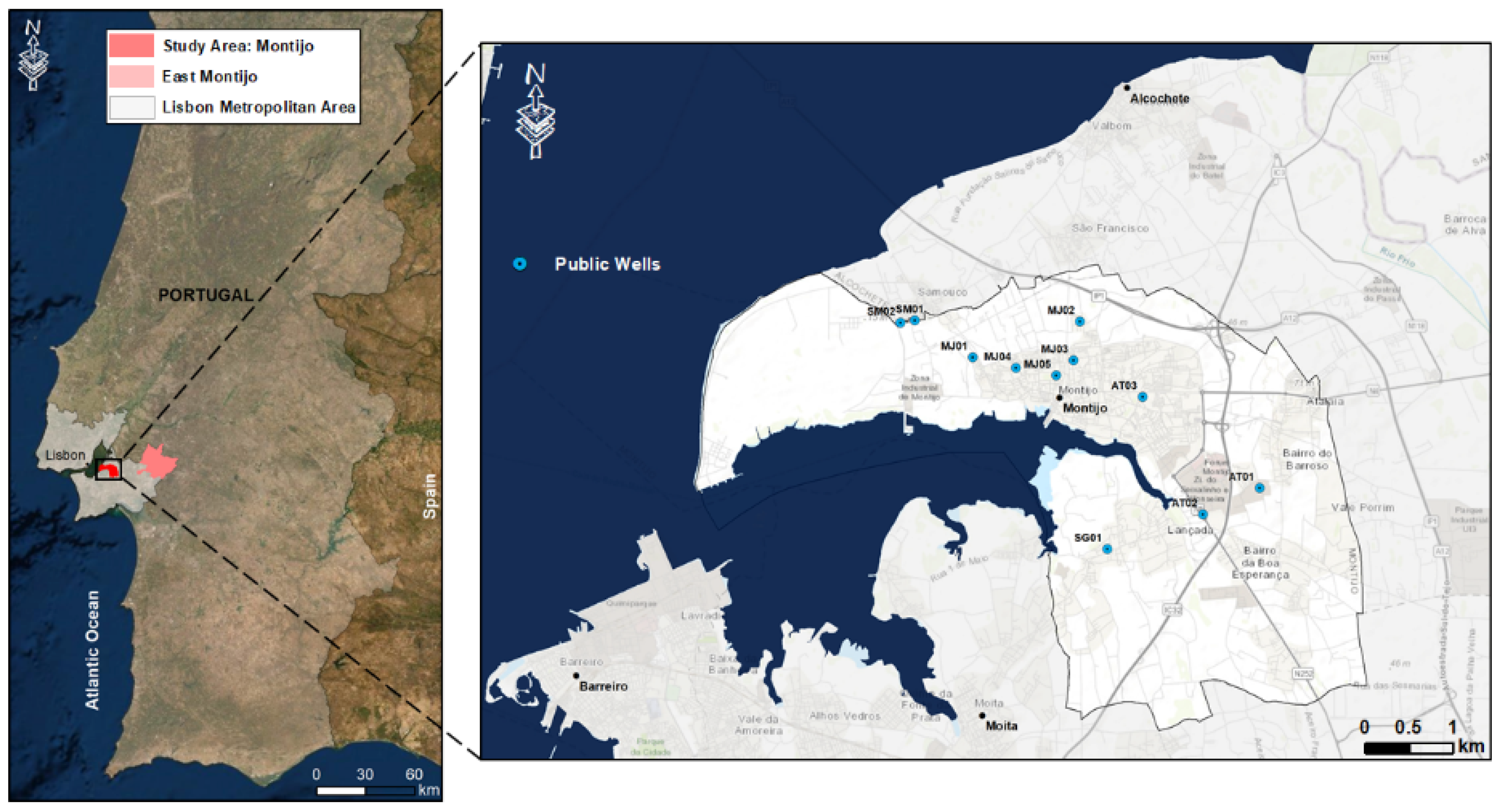
The municipality of Montijo (Portugal) is located on the south bank of the Tagus River, bordered by the Tagus Estuary, in the north of the Setubal Peninsula (Figure 1). Montijo is one of the territorially discontinuous municipalities in Portugal, and is geographically divided into two parts, western and eastern. As a result, the eastern division is not included in the study area. Within the Lisbon Metropolitan Area, Montijo (+29.7%) is among the municipalities that grew the most in terms of population between 2001 and 2011, registering 51,222 inhabitants to date (2011) [25]. More recent estimates [26], indicating that Montijo has 55,689 residents, demonstrate a new growing trend.
2.1. Geological and Hydrogeological Framework
The study area is part of the Tagus-Sado Tertiary Basin, which forms an extensive depression elongated in the northeast-southwest direction, filled by materials from peripheral zones [27,28]. The Basin is flanked to the west and north by the Mesozoic formations of the Western Rim, to the northeast and the latter by the Hercynian substrate and communicating to the south with the Atlantic Ocean, in the Setubal Peninsula [27,28]. Over time, the Basin underwent a complex evolution controlled by the interaction of tectonic and eustatic movements, which resulted in the subsidence of lands located between faults [29,30,31,32]. The movements created by the orogenic activity gave rise to several sedimentary cycles, marked by constant alternations of depositional environments, continental, marine, and brackish facies, which reveal a succession of regressive and transgressive episodes during the Neogene [16,33,34,35]. The filling of the Basin is composed of Paleogenic and Neogene deposits (Miocene and Pliocene) with thicknesses that can reach 1200 m [36,37,38,39], covered discontinuously by Quaternary sediments [27,28].
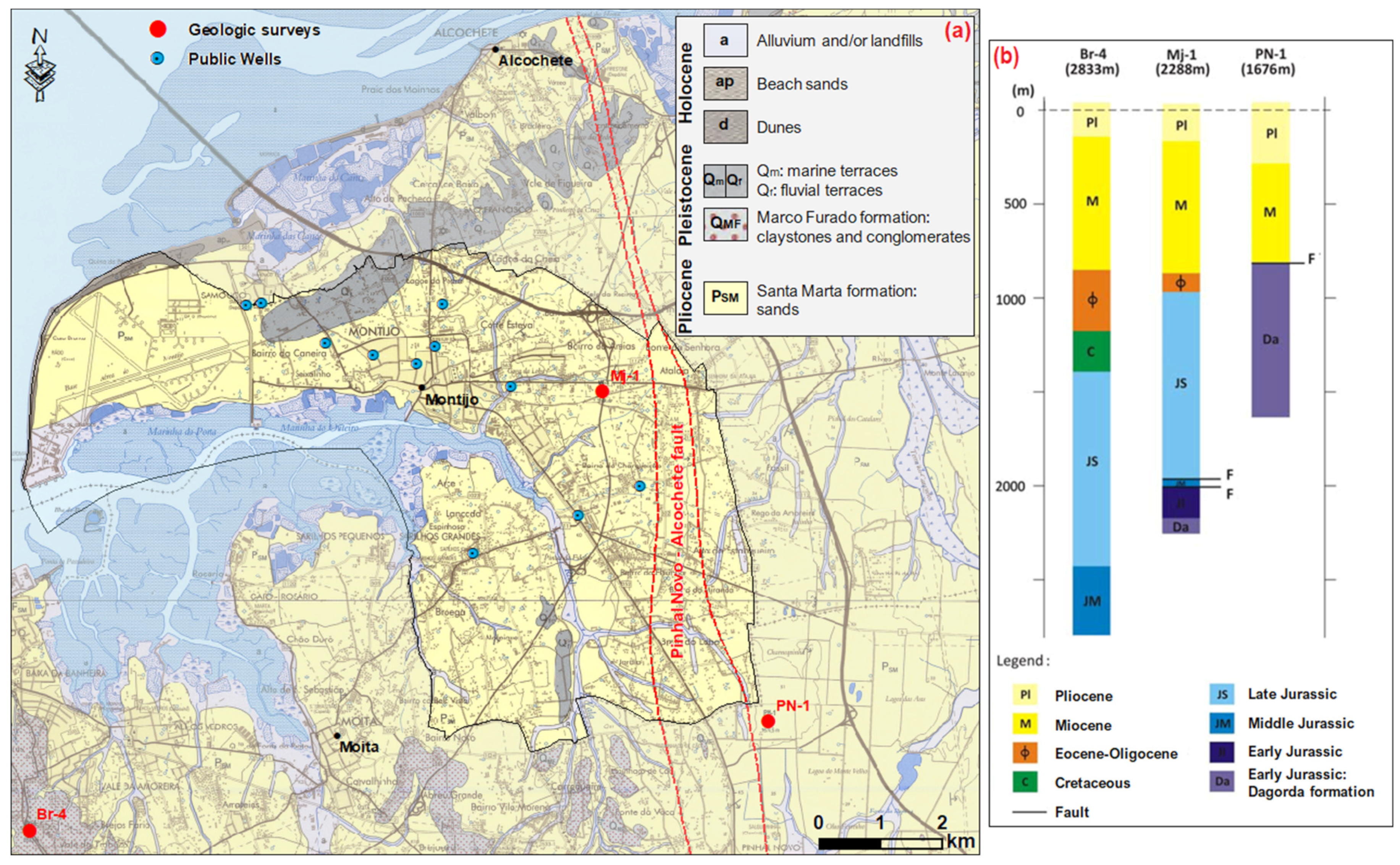
The Pliocene sands of Santa Marta dominate the landscape of the study area (Figure 2). These materials extend for more than a hundred meters of depth, being composed of sands, from fine to coarse, arkhosic, with interspersed clayey levels. Occasionally, they may be covered by alluvium and river terrace deposits, consisting essentially of clayey sludge and sand of different sizes. Pliocene sediments lie in unconformity over Miocene deposits, constituted by calcareous, bioclastic, sometimes marly sandstones [28]. These occur at depths greater than 700 m, contacting in unconformity in the Montijo area with Paleogene formations or in the Pinhal Novo area with the Dagorda Formation, from the Lower Jurassic, through the Pinhal Novo—Alcochete fault zone [40]. The fault has a predominant NNW—SSE orientation, involving a deformation zone about 2 km wide, in which it presents a pattern of branched and anastomosed faults [31,40,41,42]. An important deformation is recognized in the Pliocene sediments that implies the occurrence of further activity in the fault zone, maintaining a predominant left-facing regime, with the basal surfaces witnessing a relative descent of the eastern fault block [28,40]. We consider the fault zone as highly unproductive, being filled with black clays that contrast with the sandstone nature of the aquifer, considering the water levels measured in the field.
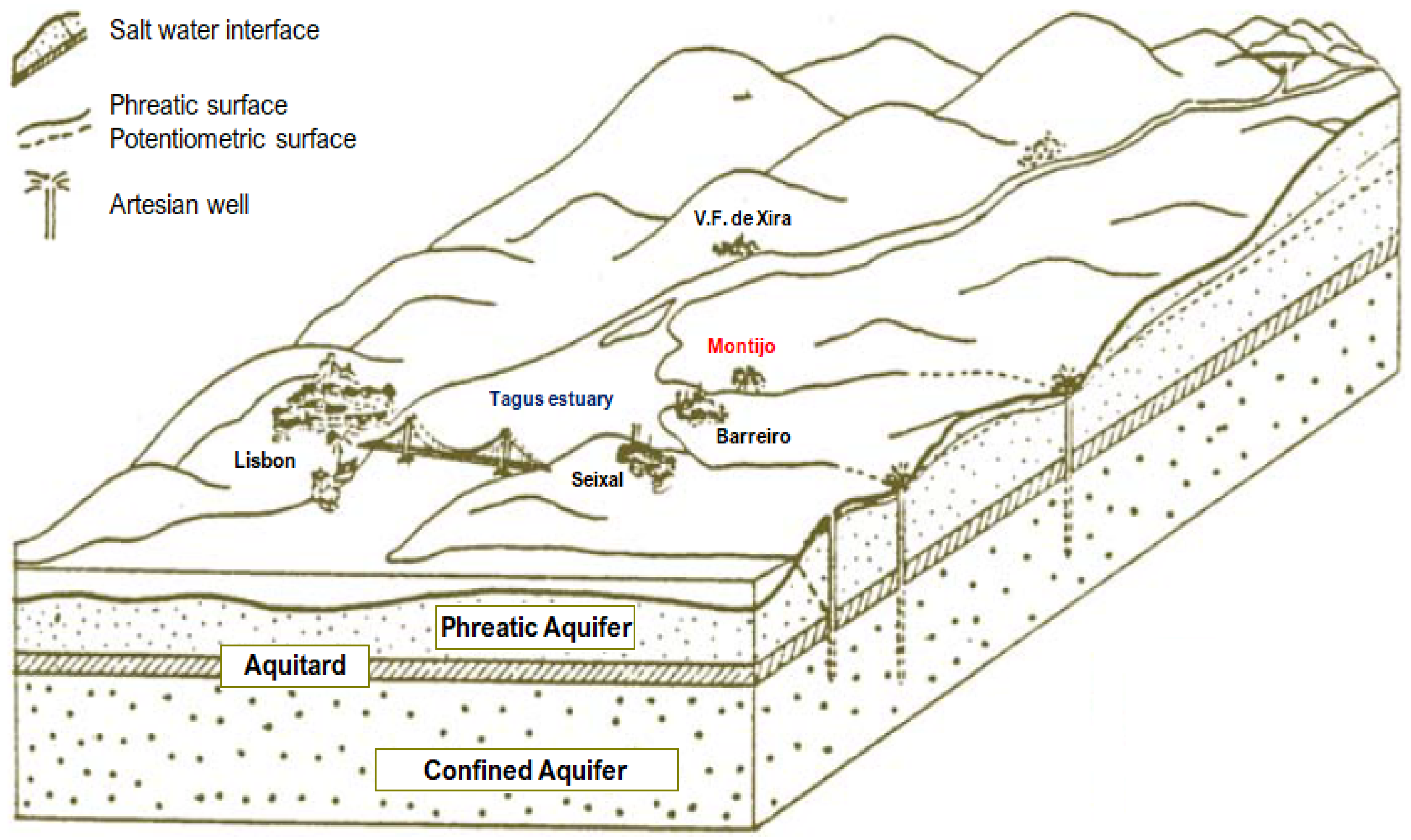
The Montijo area is part of the Tagus-Sado/Left Bank aquifer system. The system is quite complex, characterized by several lateral and vertical variations of facies that significantly alter the characteristics of the aquifer. This is formed by several porous layers, confined or semi-confined, and by clayey intercalations of low permeability [43]. In the Setubal Peninsula, the system is composed of (Figure 3): (1) an unconfined aquifer, installed in the alluvial layers of the Pleisto-Holocene and the upper layers of the Pliocene, and in hydraulic connection with the Tagus River; (2) a confined multi-layered aquifer, hosted in the Pliocene basement layers and the Late to Middle Miocene limestone layers [27,44,45]. Separating the aquifer units are semi-permeable clay lenticules that form an almost continuous aquitard level, on average at 100 m in-depth, and with varying thicknesses between 1 and 80 m [46]. At the base of the confined aquifer is a marly level that assumes an aquiclude behavior and separates this aquifer from another, deeper and of lower quality, located in the Miocene base layers [27]. Recharge occurs by direct infiltration throughout the Basin, with a higher incidence in the Pliocene and Quaternary deposits of the highlands and plateaus that border the river, yielding part of this recharge through drainage to the underlying deposits [47]. At the Basin scale (Tagus-Sado Tertiary Basin), the flow occurs preferentially, in its transverse component, towards the Tagus River, the main drainage axis, yielding discharges in the alluvium, and according to a longitudinal component, towards the Atlantic Ocean. At a regional scale (Setubal Peninsula), the Tagus estuary and its tributaries are the primary flow directions of shallow and phreatic aquifers [27,47].
2.2. Public Water Supply and Wellhead Protection Zones
The population of Montijo and Alcochete is supplied by groundwater. The public wells are divided into two water collection poles (Figure 1 and Figure 4): Samouco (SM01 and SM02) and Montijo (MJ01, MJ02, MJ03, MJ04 and MJ05). All public wells explore the sandy layers of the base of the Pliocene, along with limestone layers of the top of the Miocene. This means that they only extract in the confined aquifer, a factor that significantly reduces vulnerability. According to the United States Environmental Protection Agency (USEPA) [8], in a truly confined aquifer, the WPA around the catchment does not play any protective function, and in that case, it is sufficient to define an area immediately underneath the catchment to prevent the transport of pollutants along the catchment column. However, Moinante [48] describes some factors that may put the groundwater quality at risk, even in confined aquifers. Aquifers can present local discontinuities (facies variation, fractures, or faults), or poorly constructed or abandoned wells that may hydraulically connect several aquifers.
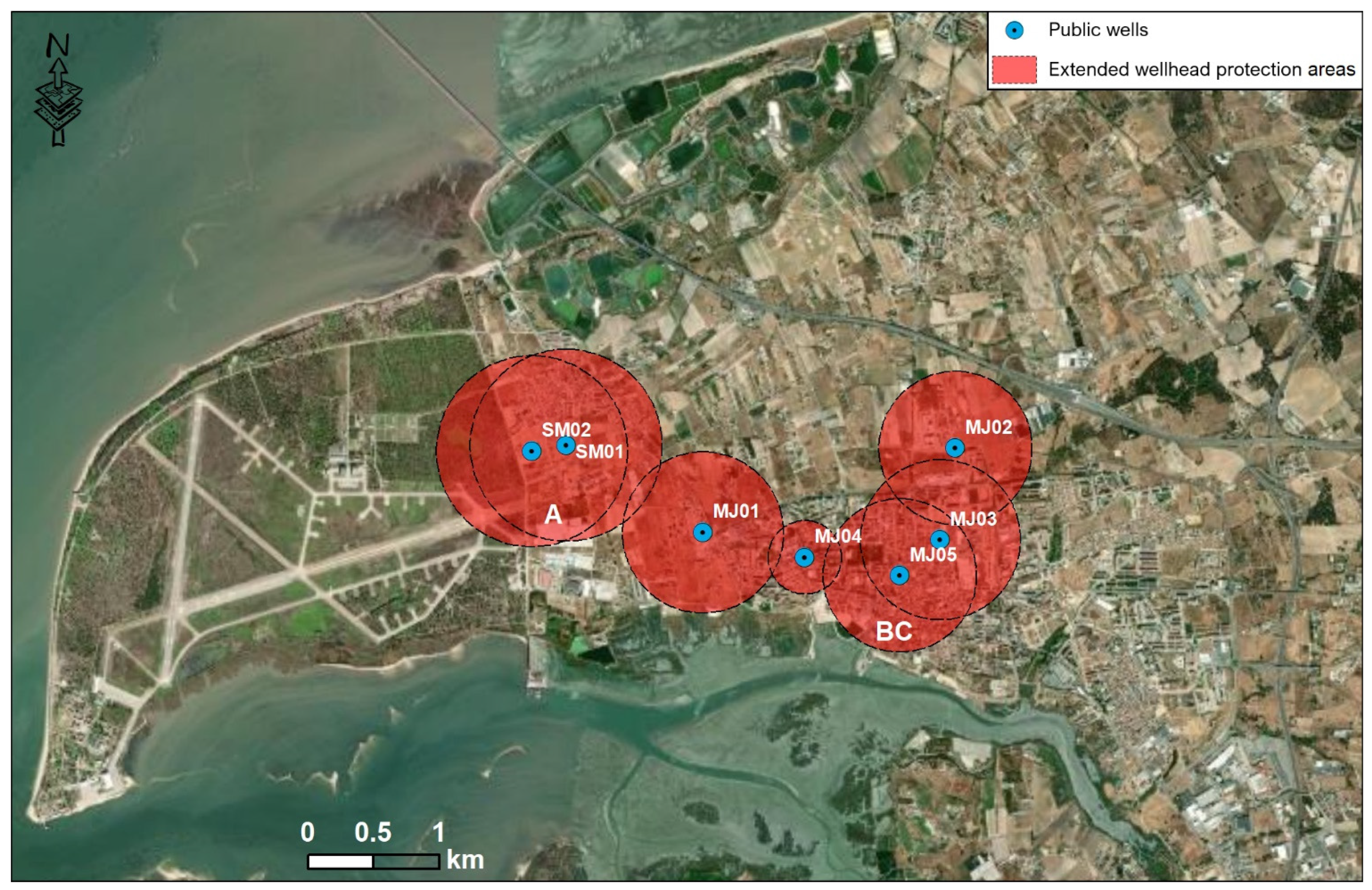
The WPAs for the public wells of Samouco and Montijo were implemented in 2009 and 2011 by the respective municipal councils (Alcochete and Montijo). These were obtained by applying three analytical methods: calculated fixed radius (CFR), Wyssling [49], and Bear and Jacobs [50]. At this time the aquifer was already exploited by several wells for public and private supply, and it was impossible to identify the regional gradient undisturbed by extractions. Therefore, the hydraulic gradient was estimated at a considerable distance from the public wells. Nevertheless, it was planned to combine the results of these three methods in the delimitation of the WPA, however, the results obtained by the Wyssling and CFR methods were poor and the Jacob and Bear method prevailed in their definition. Three extended WPAs were implemented with 2.32, 1.31, and 2.30 km2, respectively (Figure 4). The Samouco pole is not within the administrative borders of Montijo, but within those of Alcochete. However, the extended WPA (A) implemented for the two public wells in this sector is a transboundary one, mostly delimited in the study area and intercepts one of the WPA; (B) implemented in the Montijo council. A third WPA; (C) is also delimited in a neighboring municipality (Alcochete). These perimeters, including immediate and intermediate WPAs, have been in effect since 2011 and remain unchanged to this day.
Table 1 contains the hydrogeological parameters considered in the calculations. As it was not possible to measure water levels in wells in situ, the hydraulic gradients for the Samouco pole were estimated using the piezometric levels of the closest monitoring stations of the national observation network. For the Montijo pole, a complete piezometric surface of the aquifer, already affected by public and private extractions, was developed through the interpolation of the values of the piezometric levels by ordinary kriging without anisotropy. The remaining parameters were obtained in the interpretation of pumping tests. As these protection perimeters are the result of separate studies, significant differences can be observed in the values of some parameters (porosity for example), with the authors opting for different interpretations.
3. Methodology
A simple approach to analyze the long-term effectiveness of WPAs is to recalculate them at present hydrogeological conditions. Within the calculations, most of the variables remain constant, particularly the hydraulic parameters of the aquifer. However, factors such as well flow rate, piezometric levels, and hydraulic gradients are dynamic and constantly changing over time. With population growth, water demand can increase significantly and well capacity may need to be adjusted to public needs. In turn, the piezometric surface tends to suffer alterations with the continuous exploitation of the system, being able to change the hydraulic behavior of the aquifer and the natural directions of the groundwater flow. Considering the aquifer scenario in 2019, new extended WPAs were calculated using the same three analytical methods that led to the delimitation of these in 2009–2011. It is intended to review whether the perimeters in force are still valid for the current environment, maintaining the hydraulic parameters used in the previous calculations and just changing the hydraulic gradient to current values and the azimuth that represents the flow direction. The analytical methods are valid for a regional hydraulic gradient before extraction, but for this case study, as in most urban areas of the Setubal Peninsula (Portugal), it is impossible in present times to estimate the hydraulic gradient before pumping. As an alternative to analytical methods, a numerical model was developed for the case study. Using the particle tracker tool to compute the catchment areas of each public well can lead to a better solution to the problem, anticipating some limitations of the proposed analytical methods.
3.1. Analytical Methods
An automatic program developed by C. Almeida (adapted from [51]) was used to solve the mathematical equations referring to the analytical methods. This program allows calculating the WPAs, as a function of the transit time of a contaminant. Considering the same approach used to delimit the current WPA, calculations were performed for the following methods:
- (a)
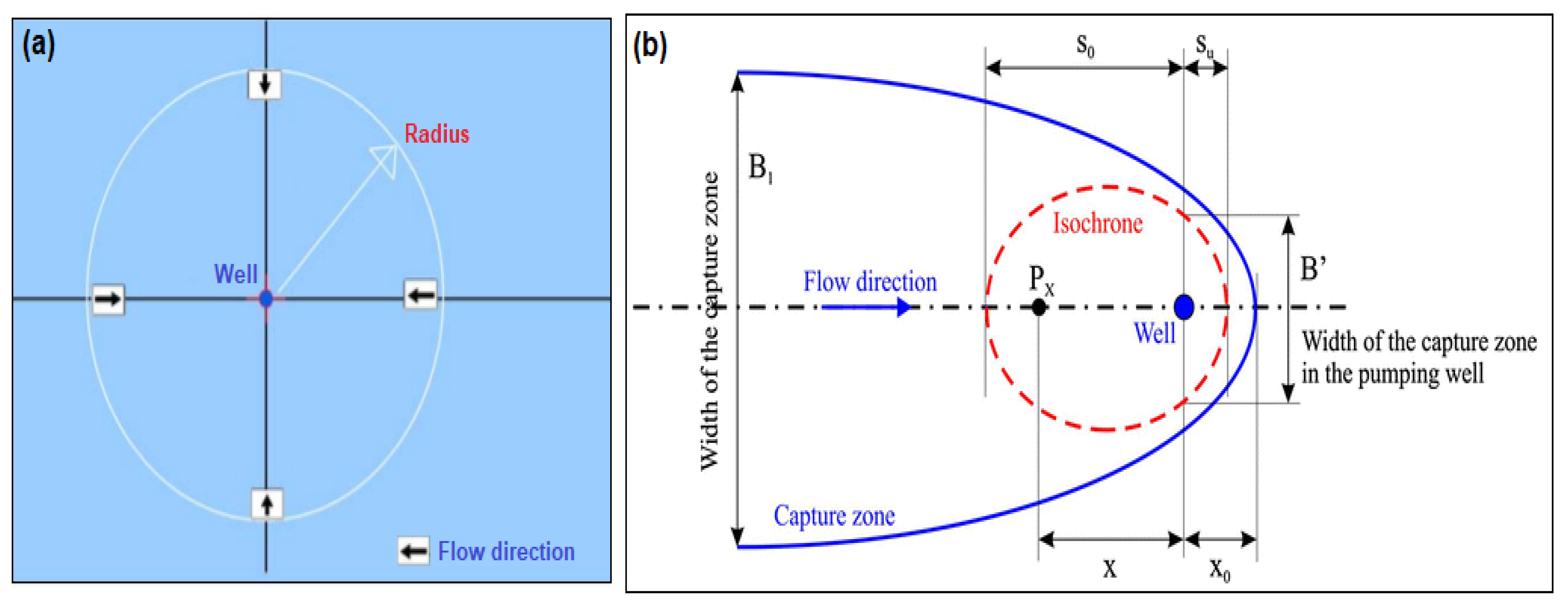
- The Fixed Radius methods (CFR) (Dec.-Law 382/99), (Figure 5) define the WPA through a volumetric equation which calculates the volume of water that reaches the catchment in a certain time, which is considered necessary to reduce the contamination to an admissible level before reaching the catchment. It is assumed that the catchment is the only draining element of the aquifer, where all flow lines converge, and that there are no privileged flow directions. In this case, the WPAs are bounded by circles around the well, with radius calculated from Equation (1), where r is the radius of WPA (m), Q is the well flow rate (m3/day), t is the time required for a pollutant to reach the well (days), n the effective porosity (%), and b is the saturated thickness (m).
- (b)
- The Wyssling method [49] (Figure 5) consists of calculating the catchment zone of a well whose size is a function of the propagation time of a contaminant in the aquifer. It is a simple method, applicable to homogeneous porous aquifers, that has the disadvantage of not considering the heterogeneities of the aquifer. The use of this method presupposes knowledge of the hydraulic gradient (i), the well capacity (Q), the hydraulic conductivity (K) or Transmissivity (T), the effective porosity (n) and the aquifer thickness (b). The variables that allow for the drawing of the WPAs are the height of the capture zone (B), the width of the capture zone front to the height of the well (B’), the capture zone radius (Xo), the Darcy velocity (V), the distance (x) corresponding to time t, in the direction of flow (upstream of capture) (So) and in the opposite direction to the flow (downstream of the catchment) (Su).
- (c)
- The Bear and Jacobs method [50] is based on the definition of the capture zone induced by the capture to be protected. A capture zone is the volume of the aquifer through which groundwater flows to a pumped well during a given time of travel. To simplify the analytical model, a series of simplifying assumptions are made. Thus, the Bear and Jacobs method is applied to the case of a single catchment located in a homogeneous, isotropic aquifer of infinite extent, subjected to a uniform regional gradient. This area is delineated using the capture zone curve. The equations for the capture zone curve were derived by Bear and Jacobs [50] and is as follows:where V represents the Darcy velocity (Equation (5); m/d), Q the flow rate (m3/day), n the effective porosity, b the aquifer thickness (m), YR, XR and tR the reduced variables, x and y the real distances (m). Equation (9) cannot be solved in an explicit form in order to XR e YR, and so iterative methods must be used. The solution was based on the method proposed by [51]. The relative Cartesian coordinates x and y are computed from Equations (10) and (11). These relative Cartesian coordinates then are rotated by the directional angle relative to the north of the hydraulic gradient translated by a distance equal to the well’s positional coordinates and converted to longitude and latitude pairs. These longitude and latitude pairs can be plotted and connected by hand but were designed to be used by a geographic information system to generate a line that can be used to delineate the WPA.
3.2. Numerical Modeling
Numerical modeling was the methodology used as an alternative to WPA calculation and to simulate the current piezometric surface of the aquifer. The exercise was carried out using the FEFLOW software [52], a three-dimensional and two-dimensional simulation tool, which uses the finite element numerical method (FEM) to solve the partial differential equations that describe the groundwater flow.
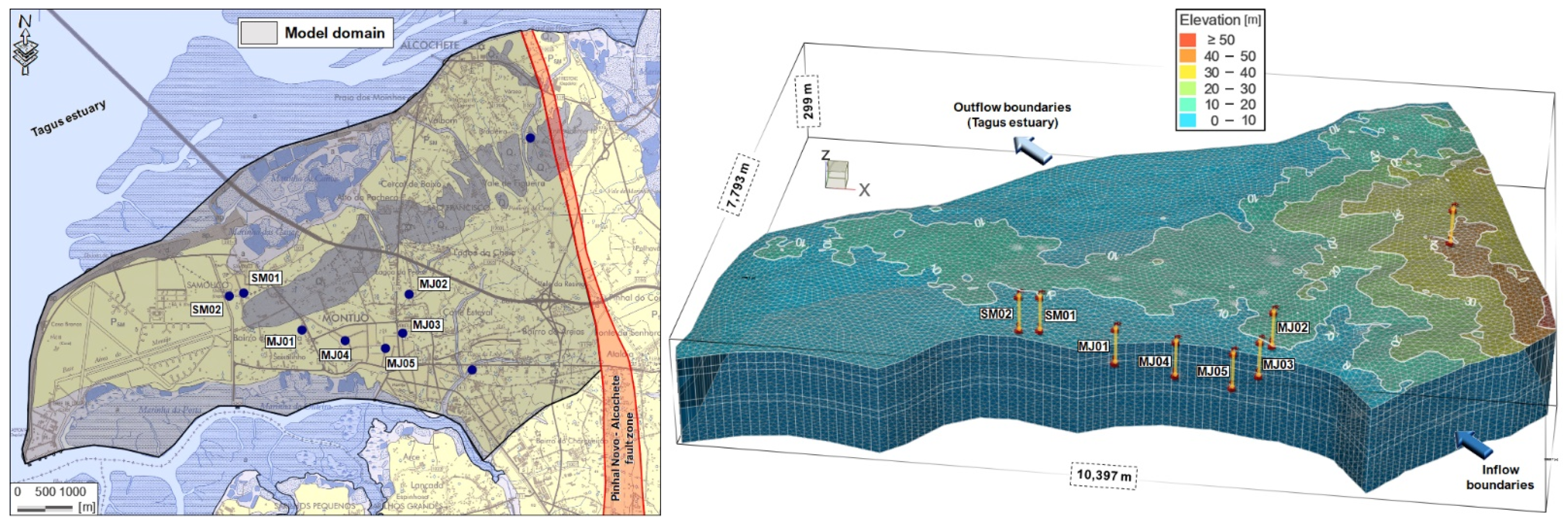
The domain of the model corresponds to a small portion of the entire aquifer system located at the northern end of the Setubal Peninsula. It is delimited by the Tagus Estuary, a discharge boundary in natural conditions, and by the Pinhal Novo—Alcochete Fault, due to the potential waterproofing in the fracture zone. The model was discretized in five layers (Figure 6) with 3 aquifer subsystems: (1) a phreatic, superficial subsystem, whose thickness should not exceed two or three tens of meters that were traditionally exploited by shallow wells; (2) an intermediate semi-confined subsystem, fully inserted in the Pliocene formations, and used mostly by private abstractions; (3) a lower confined subsystem, installed in Pliocene base deposits and upper Miocene limestone formations, and exploited by public abstractions. To separate each of the three aquifer subsystems, two aquitard-type layers were considered, allowing different flow directions for each subsystem, confinement, and the need to change the boundary conditions that characterize each layer.
Constant potential boundary conditions (Dirichlet, type 1) were imposed on the model boundaries. In the first layer (phreatic aquifer) a constant potential of 0 m was positioned in contact with the Tagus estuary, while the potential of the remaining surface water lines was defined as a function of topography (altitude). In the remaining layers, the boundary conditions are positioned to the southeast, a lateral feeding area, and to the north or northwest, in an area of potential discharge that can extend to the middle of the Tagus Estuary (Table 2). The initial conditions seek to simulate the groundwater flow in a natural regime without exploitation. The initial gradient was obtained through a set of observations of the static levels in 2019, which is quite low (0.0016). Typical of a discharge area, the hydraulic potential to the south is higher than the potential next to the estuary. The recharge in the top layer, that is, in the phreatic aquifer subsystem, was obtained through a zoning for the study area of recharge values determined by LABCARGA [53], a new methodology employed to evaluate the recharge of groundwater bodies in mainland Portugal. Due to different scales used in the geological and land use maps, data entered in the numerical model had to be slightly adjusted compared with the values obtained in that research, which spatially vary between 102 and 156 mm/year.
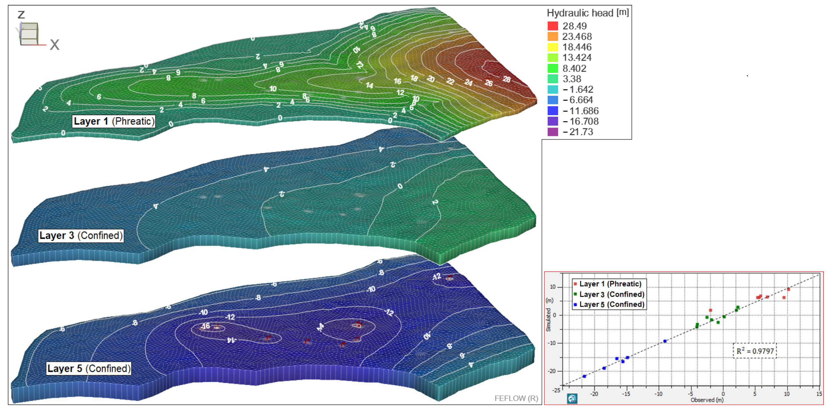
The flow rates entered in the model for each public well are the daily mean values from 2018, indicated in Table 3 as current values. It was impossible to calibrate the model with the values used to previously delimit the WPAs, also known as maximum values for a worst-case scenario. These maximum values are never reached by the abstractions, therefore they could never be used to simulate the current piezometric surface of the lower aquifer sub-system. The model calibration was based on the adjustment of boundary conditions of each aquifer, by trial and error, and calibration by the inverse method (FEPEST) of hydraulic conductivity. For this purpose, 21 observation points were selected, seven for the unconfined aquifer, eight for the intermediate subsystem, and six for the lower confined aquifer. In Figure 7 it is possible to observe the piezometric surface of the lower subsystem, captured by the public supply schemes and the main object of study of this work. The influence of water exploitation on water levels is notorious. The catchment area of the public wells is clearly drawn down in relation to the periphery, developing a radial shape flow towards these. This scenario is much more aggressive than the one observed when the WPAs were implemented. As an example, the water depth in MJ01, MJ02, and MJ03 increases from 21.5 to 33.3, 26.5 to 50.5, and 24.3 to 30.6 m, respectively, between 2011 and 2019. The continuous decrease in piezometric levels because of overexploitation of the aquifer has been a problem in several areas of the Setubal Peninsula [45,54,55].
4. Results
The results presented are divided into two chapters: analytical and numerical methods. It is important to mention that the WPAs of the Samouco pole (A) cannot be defined together with the protection perimeters of Montijo (MJ01 to MJ05), even when they intersect, since they belong to different municipal councils. On the other hand, any public well included in the extended WPAs B and C may have their perimeters delimited separately or together when they intersect.
4.1. Redefining Extended WPAs Using Analytical Methods
The hydraulic gradient (and the azimuth) is the only parameter to be changed from the previous calculations to be able to establish a comparison. In the first half of the last century, artesian wells were observed in many areas of the Setubal Peninsula [27]. Currently, due to the intensive exploitation of aquifers, drawdowns are accentuated in many urban areas.
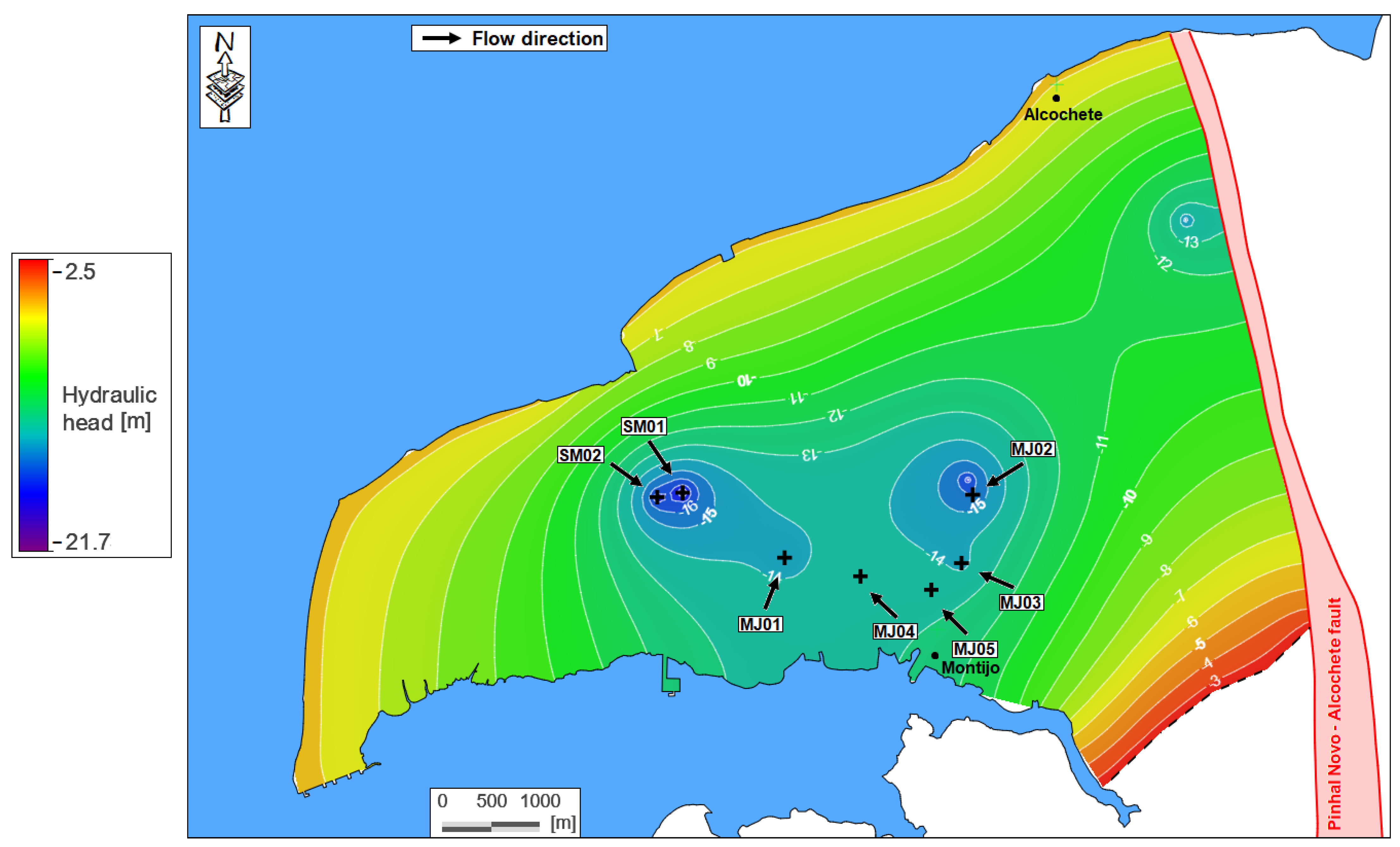
Considering that the piezometric surface presents a radial shape around the public wells, it is difficult to identify the main flow direction for the hydraulic gradient. Hence the importance of using numerical modeling first to identify the hydraulic gradient and the catchment areas of each well. In Figure 8 it is possible to observe the flow direction towards wells, for which the hydraulic gradient was calculated. The corresponding values are shown in Table 3.
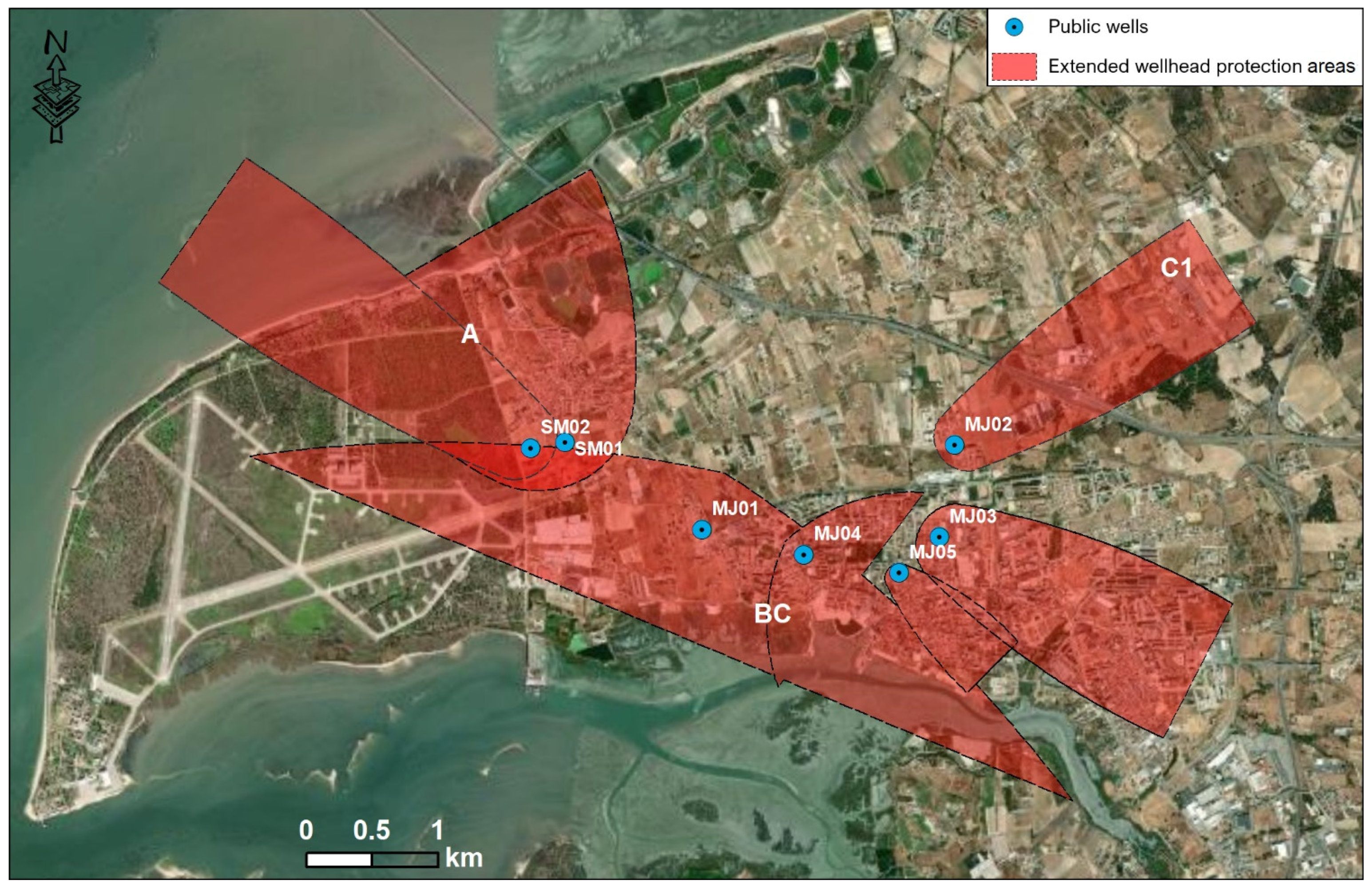
In general, the flow direction with the wells producing in 2019 is different from the one in 2011, with higher hydraulic gradients. These values were expected due to the strong drawdown observed in the last years, due to the aquifer exploitation. The greater the drawdown around the public well, the greater the hydraulic gradient generated. Considering the location of the wells, the Montijo pole is essentially fed by water from E, mostly from SE, while the Samouco pole is fed by water from NW. Together, the wells develop a joint drawdown zone, causing a depression in the piezometric surface of the aquifer in relation to less exploited areas. The well MJ01 is centered in this depression, which makes it difficult to identify the main flow direction in the surrounding area. The catchment area, visible in Figure 8, dictates that the flow is radial, although there is a slight increase towards SW, which is the direction for which the hydraulic gradient was calculated. Keeping the remaining variables constant used to determine the WPAs in 2011, the new extended WPAs were analytically calculated (Figure 9, Figure 10 and Figure 11) considering the current hydraulic gradients. The CFR method does not have the hydraulic gradient as a variable, therefore, if the flow rate (Q) is the same, the results obtained are similar to the previous ones. The Wyssling method presents interesting results if we do not consider the extended WPA obtained for well MJ01. The high flow rate together with a low hydraulic gradient and permeability produce a very flat protection area for this well. Considering that Jacob and Bear’s method was used in 2009–2011 to delimit the WPAs in force, the differences in the results obtained are substantial. The hydraulic gradient has a strong influence on the calculations, causing more elongated protection areas that almost never intersect.
4.2. Redefining Extended WPAs Using Numerical Modelling
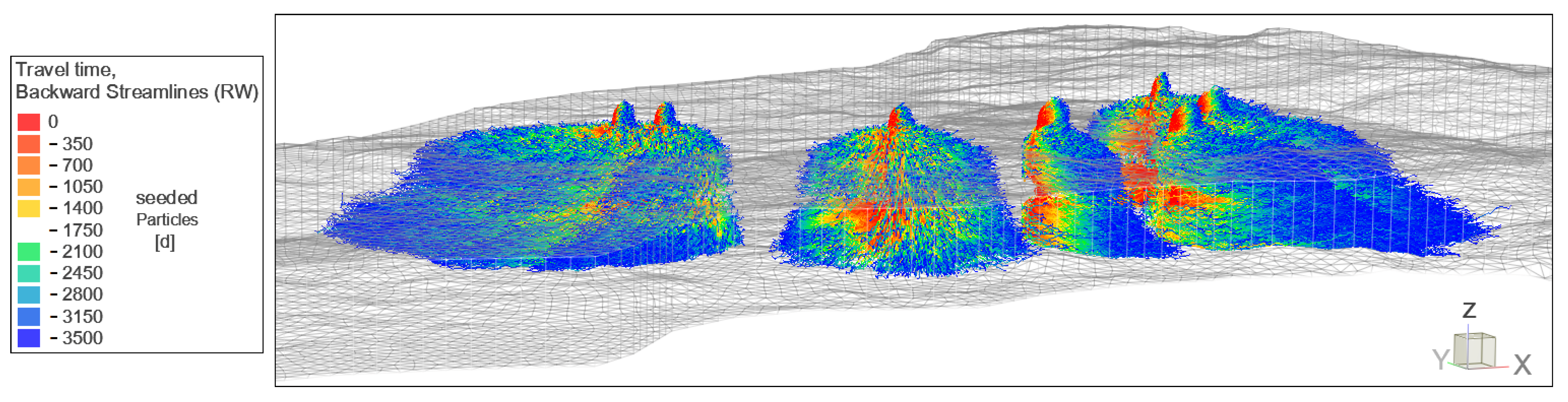
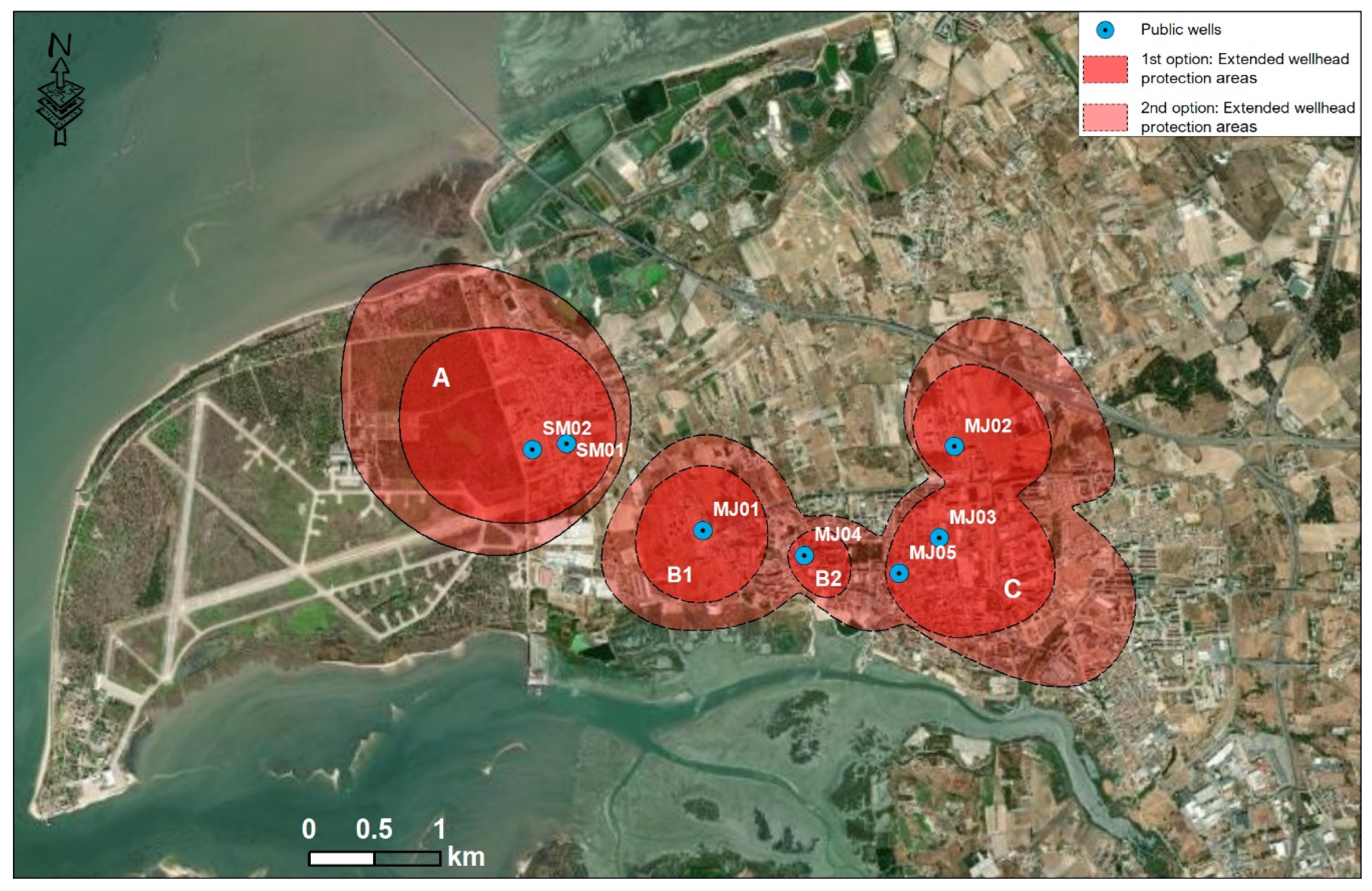
The use of a transport model dependent on the piezometric values of a flow model allows for the defining of the trajectory of particles launched at a given point. This tool is known as a particle tracker and returns a set of regressive flow lines over a time interval. Considering the flow model developed, this exercise was carried out for a period equivalent to 3500 days, which delimits the extended WPAs. The confined aquifer, the target of exploration, corresponds in numerical terms to layer 5, which is delimited by slices 5 and 6. The particle tracker performs the numerical calculations on the slices, although the hydraulic properties are assigned to the layers. The lower aquifer subsystem is represented by layer 5 but delimited by slices 5 and 6 where numerical calculations are carried out; consequently, two solutions (options) are generated. This means that in a two-dimensional perspective we have two catchment areas, one for each slice, with different dimensions. Slice 5 is superimposed by a layer of low permeability (aquitard), which significantly reduces the flow velocity, something not observed for slice 6. In Figure 12 it is possible to observe the catchment area of the seven public wells obtained in the simulation performed. The results (Figure 13) demonstrate new formats for extended WPAs and a possible division of zone B in two (1st option), although a unification between zones B and C (2nd option) is also possible, grouping all public wells in Montijo (MJ01 to MJ05). Numerical modeling offers a solution that is more compatible with the hydraulic reality of the aquifer, with protected areas more centered around the radial drawdown zones caused by public wells.
5. Discussion
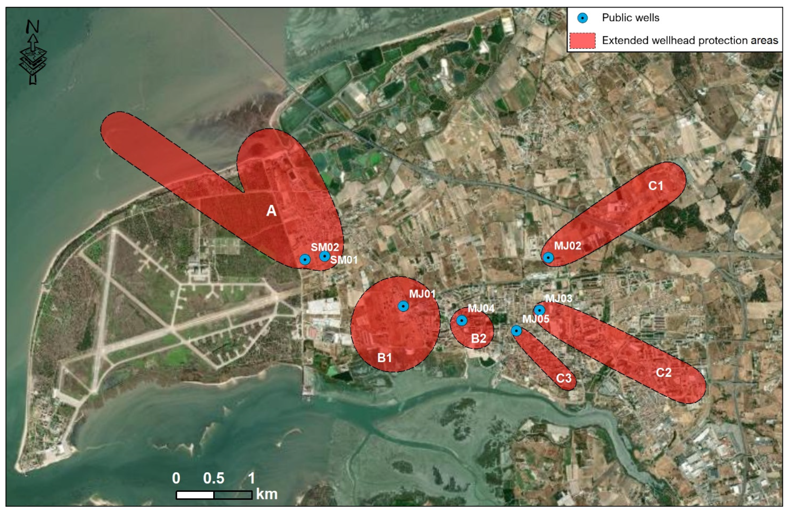
The CFR is the only method that does not depend on the hydraulic gradient for its calculation. As the properties of the aquifer do not change in this model, the results of this method could only vary if we considered another well capacity. If the flow rate increases, the protection radius and circumference also increase. Although analytical methods are only valid in non-disturbed regional gradient situations, their use here was mainly for the purpose of comparison with those calculated in 200–2011 and currently in force. The WPAs obtained for the 2019 scenario occupy a total protected area of about 5.78 km2, similar in size to the perimeters in force (5.93 km2) but with different formats in the wells MJ02 to MJ05. The extended WPAs outlined by the Wyssling method significantly increase the protection area, particularly for the Samouco public wells (SM01 and SM02) and MJ01. This method was also rejected in 2009–2011 due to poor results. The width of the catchment area presents an exaggerated dimension for these wells, given the combination of a flow rate that is too high for the hydraulic gradient in question. The Jacob and Bear method is the one that can provide a better comparison with the protection perimeters in force, given that it was the method that prevailed previously. The WPAs calculated better reflect the hydraulic gradient of the aquifer, however, the width of the protected areas is much narrower than before. Because of this, the WPA appears more individualized for each well, with single areas varying between 0.25 to 3.14 km2, for an increase in the protection area to 7.04 km2 (Table 4).
Therefore, according to the results obtained, are the extended 2009–2011 WPAs aligned with the current reality of the aquifer system? None of the analytical methods used were even close to the original solution, so it is safe to say that they are not suitable for the current situation of the aquifer. It is in the best interest to question the long-term effectiveness of these methods, particularly in urban areas where operating conditions are frequently changing. The method applied to simulate the aquifer piezometry, and consequently the hydraulic gradients, is different from the one used in 2011 (kriging). Therefore, the results may be based in this direction. Even so, both methods are valid to interpolate the piezometric levels and manage to replicate the hydraulic gradients around the catchments. It is not intended to compare methodologies here, only to simulate the piezometric surface of this aquifer.
The WPAs generated by numerical modeling consider a possible division of current zone B in two (1st option), with the protected areas varying from 0.19 km2 to 1.99 km2, adding up to a total of 4.98 km2 (Table 4). If a unification between zones B and C are considered (2nd option) the total protected area has around 10.98 km2. As with analytical methods, numerical model weight variables such as permeability, porosity, hydraulic gradient, or well capacity, also add an important parameter previously unweighted, such as recharge. It has the advantage that it is not necessary to define a uniform flow direction towards the catchment since they ponder the effects from the combined pumping wells in the hydraulic gradients and the superposition of the depression cones. Therefore, the results obtained by numerical modeling can better replicate what the extended WPAs should be for the current situation of the aquifer.
Time of travel calculations for homogenous aquifers with significant secondary porosity and heterogeneous aquifers may be significantly protected wellhead areas because hydrodynamic dispersion tends to be more significant than retardation in such aquifers. Hydrodynamic dispersion is significant in these aquifers for several reasons (1) highly permeable porous zones and fracture/conduit flow result in localized velocities that are significantly higher than the average groundwater velocity, (2) retardation processes are reduced in permeable zones (gravels, sands, fractures, conduits) because permeable aquifer materials tend to be less geochemically reactive. For example, the cation exchange capacity (CEC) of a sandy permeable zone in an aquifer will be significantly lower than the CEC of less permeable fine-grained sediments. It is necessary to choose higher-than-measured hydraulic conductivity values or use values in the upper range of similar aquifer materials when the potential for hydrodynamic dispersion is higher.
6. Conclusions
The delineation of WPA is still one of the best tools to reduce the risk of contamination, or, if it does occur, to prevent it from reaching the catchments in concentrations considered dangerous. The shape and size of the WPA depend on the hydraulic parameters of the aquifer, the flow rate of the public supply wells, and the groundwater level. Any changes of these parameters undermine the effectiveness and purpose of the WPA. With population growth in urban areas, and considering climate change, the pressure on groundwater abstraction increases. Changes in the flow direction, hydraulic behavior, and hydraulic gradients occur more often. Therefore, it is imperative to review the WPA with adequate frequency and to check its effectiveness in the medium and long term. Good governance of groundwater resources assumes the active participation of all relevant stakeholders, varying from mandated government institutions to end-users of groundwater and those who value groundwater-related ecosystems.
In the present case study, the hydraulic gradients of the aquifer changed from 0.0005–0.002 in 2009–2011, to 0.0008–0.008 in 2019, and consequently the direction of the groundwater flow in some areas. New WPA must be defined, however, integrated methodologies are needed for the delimitation of the new protected areas, taking into consideration the already established land use in the city. The WPAs delineated by the CFR method do not provide adequate protection. The Wyssling method calculates very large areas, particularly in cases where the hydraulic gradients are low. The Jacob and Bear method may be a valid solution. However, there is no uniform flow direction towards the wells, as these methods require, and the local hydraulic gradients are affected by neighboring wells. The best protection of the public supply wells seems to be obtained through numerical modeling. In a balance between well protection and land use, i.e., to maintain the quality of the water captured in the wells and at the same time not creating problems in the land use planning, the best WPA delineation for the current scenario is represented in Figure 13. Considering the two proposed solutions, the protected areas can range from four smaller zones with a total of 4.98 km2 to two larger zones with 10.24 km2.
Many WPA for public supply were and are delineated by analytical methods; however, situations where the wells are in aquifers with piezometry not affected by other extractions should be rare. The best methodology for delineating the WPA is using numerical flow modelling together with particle tracking simulation. This method considers intrinsic aquifer parameters, but also the water balance. Considering that aquifer recharge is an important factor in the infiltration and transport of contaminants into the aquifer, any methodology for estimating WPAs should consider it and not only parameters that influence the movement of contaminants within the aquifer. In urban areas, where the hydrostatic level concept no longer applies and the catchment areas of public wells overlap each other, numerical modeling may even be the only viable solution. Once the model is built, it can be reused multiple times, varying only the exploration conditions, with the opening of new wells or the increase/decrease in the well’s capacity.
Thus, the combination of WPA methods, preferably based on groundwater flow models, with methodologies for assessing the vulnerability of aquifers to contamination seems to be a good solution. The effectiveness of the WPA should also be verified through a close monitoring of the physical-chemical composition of the abstracted water, either at the abstraction itself or at sampling points (piezometers, boreholes, wells) within the WPA.
Author Contributions
All the authors contributed to the write of the paper. This paper was completed under the supervision of M.d.R.C., J.M.C. and C.A.; J.Z. conducted the calculation and numerical modeling, figures, and analyzed the results and wrote the paper; C.A. developed a software for analytical methods; M.P. contributed to the analysis discussion; M.d.R.C. helped with reviewing the manuscript. All authors have read and agreed to the published version of the manuscript.
Funding
This research received no external funding.
Acknowledgments
The authors are grateful for the financial support of the Portuguese Environment Agency (APA) and Portuguese Foundation for Science and Technology (FCT) projects (UIDB/50019/2020-IDL). This study was carried out partially under the framework of the Labcarga|ISEP re-equipment program (IPP-ISEP|PAD’2007/08) and GeoBioTec|UA (UID/GEO/04035/2020). We acknowledge the anonymous reviewers and editors for their constructive comments which helped to improve the focus of the manuscript.
Conflicts of Interest
The authors declare that they have no conflict of interest.
References
- UNESCO World Water Assessment Programme. The United Nations World Water Development Report 2021: Valuing Water; UNESCO: Paris, France, 2021; p. 187. ISBN 978-92-3-100434-6. [Google Scholar]
- Martínez Navarrete, C.; Grima Olmedo, J.; Durán Valsero, J.J.; Gómez Gómez, J.D.; Luque Espinar, J.A.; de la Orden Gómez, J.A. Groundwater protection in Mediterranean countries after the European water framework directive. Environ. Geol. 2008, 54, 537–549. [Google Scholar] [CrossRef]
- Boretti, A.; Rosa, L. Reassessing the projections of the World Water Development Report. NPJ Clean Water 2019, 2, 15. [Google Scholar] [CrossRef]
- Herbert, C.; Döll, P. Global Assessment of Current and Future Groundwater Stress with a Focus on Transboundary Aquifers. Water Resour. Res. 2019, 55, 4760–4784. [Google Scholar] [CrossRef]
- Bertrand, G.; Hirata, R.; Pauwels, H.; Cary, L.; Petelet-Giraud, E.; Chatton, E.; Aquilina, L.; Labasque, T.; Martins, V.; Montenegro, S.; et al. Groundwater contamination in coastal urban areas: Anthropogenic pressure and natural attenuation processes. Example of Recife (PE State, NE Brazil). J. Contam. Hydrol. 2016, 192, 165–180. [Google Scholar] [CrossRef] [PubMed]
- Shultz, S.D.; Lindsay, B.E. The willingness to pay for groundwater protection. Water Resour. Res. 1990, 26, 1869–1875. [Google Scholar] [CrossRef]
- Velis, M.; Conti, K.I.; Biermann, F. Groundwater and human development: Synergies and trade-offs within the context of the sustainable development goals. Sustain. Sci. 2017, 12, 1007–1017. [Google Scholar] [CrossRef] [PubMed] [Green Version]
- U.S. Environmental Protection Agency. 1987 Final Rule: Emergency and Hazardous Chemical Inventory Forms and Community Right-To-Know Reporting Requirements 52 FR 38344. Available online: https://www.epa.gov/sites/default/files/2013-09/documents/52fr38364.pdf (accessed on 7 February 2022).
- EU—European Commission. Report from the Commission. Implementation of Council Directive 91/676/EEC Concerning the Protection of Waters against Pollution Caused by Nitrates from Agricultural Sources. Synthesis from Year 2000 Member States Reports. Available online: https://eur-lex.europa.eu/legal-content/EN/TXT/PDF/?uri=CELEX:52002DC0407&from=EN (accessed on 7 February 2022).
- Colon, M.; Richard, S.; Roche, P.A. The evolution of water governance in France from the 1960s: Disputes as major drivers for radical changes within a consensual framework. Water Int. 2018, 43, 109–132. [Google Scholar] [CrossRef]
- García-García, A.; Martínez-Navarrete, C. Protection of groundwater intended for human consumption in the water framework directive: Strategies and regulations applied in some European countries. Pol. Geol. Inst. Spec. Pap. 2005, 18, 28–32. Available online: https://www.pgi.gov.pl/en/docman-tree-all/publikacje-2/special-papers/79-garcia/file.html (accessed on 2 February 2022).
- Cleary, T.; Cleary, R.W. Delineation of Wellhead Protection Areas: Theory and Practice. Water Sci. Technol. 1991, 24, 239–250. [Google Scholar] [CrossRef]
- Taylor, R.; Cronin, A.; Pedley, S.; Barker, J.; Atkinson, T. The implications of groundwater velocity variations on microbial transport and wellhead protection—Review of field evidence. FEMS Microbiol. Ecol. 2004, 49, 17–26. [Google Scholar] [CrossRef] [PubMed] [Green Version]
- Foster, S.; Hirata, R.; Gomes, D.; Paris, M.; D’Elia, M. Groundwater Quality Protection—A Guide for Water Utilities, Municipal Authorities, and Environment Agencies; World Bank GW-MATe Report 2007; World Bank: Washington, DC, USA, 2007; ISBN 0-8213-4951-1. [Google Scholar]
- Fileccia, A. Some simple procedures for the calculation of the influence radius and well head protection areas (theoretical approach and a field case for a water table aquifer in an alluvial plain). Acque Sotter. Ital. J. Groundw. 2015, 4, 7–23. [Google Scholar] [CrossRef]
- Liu, Y.; Weisbrod, N.; Yakirevich, A. Comparative Study of Methods for Delineating the Wellhead Protection Area in an Unconfined Coastal Aquifer. Water 2019, 11, 1168. [Google Scholar] [CrossRef] [Green Version]
- Krijgsman, B.; Lobo-Ferreira, J.P.C. A Methodology for Delineating Wellhead Protection Areas; INCH 7; Laboratório Nacional de Engenharia Civil: Lisbon, Portugal, 2001; ISBN 972-49-1882-3. [Google Scholar]
- Expósito, J.L.; Esteller, M.V.; Paredes, J.; Rico, C.; Franco, R. Groundwater Protection Using Vulnerability Maps and Wellhead Protection Area (WHPA): A Case Study in Mexico. Water Resour. Manag. 2010, 24, 4219–4236. [Google Scholar] [CrossRef] [Green Version]
- Piccinini, L.; Fabbri, P.; Pola, M.; Marcolongo, E. Numerical modeling to well-head protection area delineation, an example in Veneto Region (NE Italy). Rend. Online Soc. Geol. Ital. 2015, 35, 232–235. [Google Scholar] [CrossRef]
- Thibaut, R.; Laloy, E.; Hermans, T. A new framework for experimental design using Bayesian Evidential Learning: The case of wellhead protection area. J. Hydrol. 2021, 603, 126903. [Google Scholar] [CrossRef]
- Ramanarayanan, T.S.; Storm, D.E.; Smolen, M.D. Seasonal Pumping Variation Effects on Wellhead Protection Area Delineation. Water Resour. Bull. 1995, 31, 421–430. [Google Scholar] [CrossRef]
- Tosco, T.; Sethi, R. Comparison between backward probability and particle tracking methods for the delineation of well head protection areas. Environ. Fluid Mech. 2010, 10, 77–90. [Google Scholar] [CrossRef]
- Evers, S.; Lerner, D.N. How Uncertain Is Our Estimate of a Wellhead Protection Zone? Groundwater 2005, 36, 49–57. [Google Scholar] [CrossRef]
- Theodossiou, N.; Fotopoulou, E. Delineating well-head protection areas under conditions of hydrogeological uncertainty. A case-study application in northern Greece. Environ. Process. 2015, 2, 113–122. [Google Scholar] [CrossRef]
- INE. Censos 2011 Resultados Definitivos—Região Lisboa. Available online: https://censos.ine.pt/ngt_server/attachfileu.jsp?look_parentBoui=156652050&att_display=n&att_download=y (accessed on 18 January 2022).
- INE. Censos 2021 Resultados Provisórios. Available online: https://www.ine.pt/ngt_server/attachfileu.jsp?look_parentBoui=536757700&att_display=n&att_download=y (accessed on 18 January 2022).
- Almeida, C.; Mendonça, J.J.L.; Jesus, M.R.; Gomes, A.J. Sistemas Aquíferos de Portugal Continental; Centro de Geologia da Universidade de Lisboa; Instituto Nacional da Água: Lisboa, Portugal, 2000. [Google Scholar] [CrossRef]
- Pais, J.; Moniz, C.; Cabral, J.; Cardoso, J.; Legoinha, P.; Machado, S.; Morais, M.A.; Lourenço, C.; Ribeiro, M.L.; Henriques, P.; et al. Notícia Explicativa da Carta Geológica 1:50.000, nº 34-D, Lisboa; Instituto Nacional de Engenharia, Tecnologia e Inovação: Lisboa, Portugal, 2006; Available online: https://novaresearch.unl.pt/en/publications/not%C3%ADcia-explicativa-da-carta-geol%C3%B3gica-150000-n%C2%BA-34-d-lisboa (accessed on 15 December 2021).
- Galopim de Carvalho, A.; Ribeiro, A.; Cabral, J. Evolução Paleogeográfica da Bacia Cenozoica do Tejo-Sado; Boletim da Sociedade Geológica de Portugal: Lisboa, Portugal, 1983–1985; Volume XXIV, pp. 209–212. Available online: https://www.researchgate.net/publication/292390457_Evolucao_paleogeografica_da_bacia_cenozoica_do_Tejo-Sado (accessed on 10 December 2021).
- Kullberg, M.C.; Kullberg, J.C.; Terrinha, P. Tectónica da Cadeia da Arrábida. In Tectónica das Regiões de Sintra e Arrábida. Memórias Geociências; Museu Nacional de História Natural, Universidade de Lisboa: Lisboa, Portugal, 2000; pp. 35–84. Available online: https://research.unl.pt/ws/portalfiles/portal/325791/Kullberg+et+al+%28Mem+Geoc+MNHN+2000%29.pdf (accessed on 10 December 2021).
- Kullberg, J.C.; Rocha, R.B.; Soares, A.F.; Rey, J.; Terrinha, P.; Callapez, P.; Martins, L. A Bacia Lusitaniana: Estratigrafia, Paleogeografia e Tectónica. In Geologia de Portugal no Contexto da Ibéria; Dias, R., Araújo, A., Terrinha, P., Kullberg, J.C., Eds.; Universidade de Évora: Évora, Portugal, 2006; pp. 317–368. Available online: http://hdl.handle.net/10362/1487 (accessed on 10 December 2021).
- Kullberg, J.C.; Rocha, R.B.; Soares, A.F.; Rey, J.; Terrinha, P.; Azerêdo, A.C.; Callapez, P.; Duarte, L.V.; Kullberg, M.C.; Martins, L.; et al. A Bacia Lusitaniana: Estratigrafia, Paleogeografia e Tectónica. In Geologia de Portugal; Dias, R., Araújo, A., Terrinha, P., Kullberg, J.C., Eds.; Escolar Editora: Lisboa, Portugal, Volume II—Geologia Meso-cenozóica de Portugal; pp. 195–347. Available online: https://docentes.fct.unl.pt/omateus/files/kullberg_et_al_2013_a_bacia_lusitaniana.pdf (accessed on 10 December 2021).
- Antunes, M.T.; Elderfield, H.; Legoinha, P.; Pais, J. A stratigraphic framework for the Miocene from the Lower Tagus Basin (Lisbon, Setúbal Peninsula, Portugal): Depositional sequences, biostratigraphy and isotopic ages. Rev. Soc. Geológica España 1999, 12, 3–15. Available online: https://run.unl.pt/handle/10362/4167 (accessed on 15 December 2021).
- Antunes, M.T.; Legoinha, P.; Cunha, P.; Pais, J. High resolution stratigraphy and Miocene facies correlation in Lisbon and Setúbal Peninsula (Lower Tagus basin, Portugal). Ciências Da Terra 2000, 14, 183–190. Available online: http://hdl.handle.net/10362/4707 (accessed on 15 December 2021).
- Cunha, P.; Pais, J.; Legoinha, P. Evolução geológica de Portugal continental durante o Cenozóico—Sedimentação aluvial e marinha numa margem continental passiva (Ibéria ocidental). In Proceedings of the 6th Symposium on the Atlantic Iberian Margin, Oviedo, Spain, 1–5 December 2009; Available online: https://run.unl.pt/handle/10362/2351 (accessed on 15 December 2021).
- Antunes, M.T.; Chevalier, J.P. Notes sur la Géologie et la Paléontologie du Miocène de Lisbonne—VII—Observations compémentaires sur les madréporaires et les faciès rècifaux. Rev. Fac. Ciências Lisb. 1971, 16, 291–305. [Google Scholar]
- Mendes-Victor, L.A.; Hirn, A.; Veinante, J.L. A seismic section across the Tagus valley, Portugal: Possible evolution of the crust. Ann. Géophysique 1980, 36, 469–476. [Google Scholar]
- Azevedo, T.M. O Sinclinal de Albufeira. Evolução Pós-Miocénica e Reconstituição Paleogeográfica. Ph.D. Thesis, Centro de Geologia da Faculdade de Ciências de Lisboa, Lisboa, Portugal, 1982. [Google Scholar]
- Pais, J. The Neogene of the Lower Tagus Basin (Portugal). Rev. Esp. Paleontol. 2004, 19, 229–242. [Google Scholar] [CrossRef]
- Moniz, C. Contributo para o conhecimento da Falha de Pinhal Novo—Alcochete, no âmbito da Neotectónica do Vale Inferior do Tejo. Master’s Thesis, Faculdade de Ciências da Universidade de Lisboa, Lisbon, Portugal, 2010. [Google Scholar]
- Ribeiro, A.; Kullberg, M.C.; Kullberg, J.C.; Manuppella, G.; Phipps, S. A review of Alpine tectonics in Portugal: Foreland datachment in basement and cover rocks. Tectonophysics 1990, 184, 357–366. Available online: https://repositorio.lneg.pt/handle/10400.9/1877 (accessed on 10 December 2021). [CrossRef] [Green Version]
- Cabral, J.; Moniz, C.; Ribeiro, P.; Terrinha, P.; Matias, L. Analysis of seismic reflection data as a tool for the seismotectonic assessment of a low activity intraplate basin—The Lower Tagus Valley (Portugal). J. Seismol. 2003, 7, 431–447. [Google Scholar] [CrossRef]
- Simões, M. Contribuição Para o Conhecimento Hidrogeológico do Cenozóico na Bacia do Baixo Tejo. Ph.D. Thesis, Universidade Nova de Lisboa, Caparica, Portugal, 1998. [Google Scholar]
- PNUD—Programme Des Nations Unies Pour Le Developpement. Étude des Eaux Souterraines de la Péninsule de Setúbal (Système Aquifère Mio-Pliocène du Tejo et du Sado); Rapport Final sur les Résultats du Project, Conclusions et Recommendations; Programme des Nations Unies Pour le Développement; Direcção Geral dos Recursos e Aproveitamentos Hidráulicos: Lisbon, Portugal, 1981. [Google Scholar]
- Zeferino, J. Modelação Numérica (FEFLOW) e Contaminação por Intrusão Salina do Sistema Aquífero Mio-Pliocénico do Tejo, na Frente Ribeirinha do Barreiro. Master’s Thesis, Faculdade de Ciências e Tecnologia Universidade Nova de Lisboa, Caparica, Portugal, 2016. [Google Scholar]
- HP—Hidrotécnica Portuguesa. Estudo de Caracterização dos Aquíferos e dos Consumos de Água na Península de Setúbal; Estudo Realizado Para Empresa Portuguesa de Águas Livres, S.A., (EPAL): Lisbon, Portugal, 1994. [Google Scholar]
- Lopo Mendonça, J.P. Caracterização geológica e hidrogeológica da Bacia Terciária do Tejo-Sado. In Tágides 7, Os Aquíferos das Bacias Hidrográficas do Rio Tejo e das Ribeiras do Oeste, Saberes e Reflexões; ARH do Tejo, I.P.: Lisbon, Portugal, 2010; pp. 59–65. Available online: https://www.researchgate.net/publication/307205223_Caracterizacao_geologica_e_hidrogeologica_da_bacia_terciaria_do_Tejo_Sado (accessed on 12 December 2021).
- Moinante, M.J. Delimitação de Perímetros de Protecção de Captações de Águas Subterrâneas. Estudo Comparativo Utilizando Métodos Analíticos E Numéricos. Master’s Thesis, Universidade Técnica de Lisboa, Lisbon, Portugal, 2003. [Google Scholar]
- Wyssling, L. Eine nene form el zur Berechnung der Zustromungsdaner der grunduaners zu einem Grunduaner Pumpuern. Eclogee Geol. Helv. 1979, 72, 401–406. [Google Scholar]
- Bear, J.; Jacobs, M. On the Movement of Water Bodies Injected into Aquifer. J. Hydrol. 1965, 3, 37–57. [Google Scholar] [CrossRef]
- McElwee, C.D. Capture zones for simple aquifers. Ground Water 1991, 29, 587–590. Available online: https://pubs.er.usgs.gov/publication/70016701 (accessed on 8 January 2022). [CrossRef]
- Diersch, H.J. FEFLOW: Finite Element Modeling of Flow, Mass and Heat Transport in Porous and Fractured Media; Springer: Berlin/Heidelberg, Germany, 2014. [Google Scholar] [CrossRef]
- LABCARGA. Desenvolvimento de Métodos Específicos Para a Avaliação da Recarga das Massas de Água Subterrâneas, Para Melhorar a Avaliação do Estado Quantitativo; Relatório Final; Laboratório de Cartografia e Geologia Aplicada: Porto, Portugal, 2017; 141p. [Google Scholar]
- Simões, M. Modelos e Balanços do Aquífero Sedimentar da Bacia do Tejo—Margem Esquerda, na Península de Setúbal. In Proceedings of the 8º Seminário Sobre Águas Subterrâneas, FCUL, Lisbon, Portugal, 10–11 March 2011; pp. 119–122. Available online: https://novaresearch.unl.pt/en/publications/pmodelos-e-balan%C3%A7os-do-aqu%C3%ADfero-sedimentar-da-bacia-do-tejo-marge (accessed on 10 September 2021).
- Gonçalves, P. Sustentabilidade do Aquífero Tejo-Sado (Exploração eficiente na Margem Sul do Tejo). In Proceedings of the 12º Seminário Sobre Águas Subterrâneas, Coimbra, Portugal, 7–8 March 2019; Livro de Atas. Universidade de Coimbra: Coimbra, Portugal, 2019. [Google Scholar]
Figure 1.
Geographical framework of the study area and location of the public wells supply.

Figure 2.
(a) Geological framework of the study area on sheet 34-D (Lisbon) of the Geological Chart of Portugal at 1:50,000 scale, (b) Synthetic stratigraphic columns from deep wells in the northern sector of the Setubal Peninsula [40].
Figure 2.
(a) Geological framework of the study area on sheet 34-D (Lisbon) of the Geological Chart of Portugal at 1:50,000 scale, (b) Synthetic stratigraphic columns from deep wells in the northern sector of the Setubal Peninsula [40].

Figure 3.
Schematic three-dimensional representation (conceptual model) of the Tagus-Sado Mio-Pliocene aquifer system [31].
Figure 3.
Schematic three-dimensional representation (conceptual model) of the Tagus-Sado Mio-Pliocene aquifer system [31].

Figure 4.
Current extended wellhead protection areas.

Figure 5.
(a) The Fixed Radius methods and (b) WPA according to Wyssling’s method [2].
Figure 5.
(a) The Fixed Radius methods and (b) WPA according to Wyssling’s method [2].

Figure 6.
Schematic representation of the model domain in two and three dimensions.

Figure 7.
Groundwater flow model and calibration values.

Figure 8.
Piezometric surface of confined aquifer and main flow direction captured by public wells.

Figure 9.
Extended wellhead protection zones delimited by the Fixed Radius method.

Figure 10.
Extended wellhead protection zones delimited by the Wyssling method.

Figure 11.
Extended wellhead protection zones delimited by the Jacob and Bear method.

Figure 12.
Using the particle tracker to calculate a catchment area for public wells in 3500 days.

Figure 13.
Extended wellhead protection zones calculated by numerical modelling.


Table 1.
Hydrogeological parameters and wells technical features used in the application of analytical methods to calculate the WPAs in force.
Table 1.
Hydrogeological parameters and wells technical features used in the application of analytical methods to calculate the WPAs in force.
| Extended WPZ | Area (km2) | Wells | Drains (m) | Flow Rate (m3/Day) | Hydraulic Gradient | Aquifer Thickness (m) | Transmissivity (m2/Day) | Hydraulic Conductivity (m/Day) | Porosity |
|---|---|---|---|---|---|---|---|---|---|
| A | 2.32 | SM01 | 206–259 | 3456 | 0.001–0.0008 | 72 | 370 | 5 | 0.10 |
| SM02 | 185–273 | 5184 | 109 | 1140 | 10 | ||||
| B | 1.31 | MJ01 | 110–220 | 3636 | 0.00047 | 43 | 614 | 14 | 0.25 |
| MJ04 | 121–233 | 774 | 0.00130 | 44 | 1008 | 23 | |||
| C | 2.30 | MJ02 | 141–248 | 3289 | 0.00203 | 43 | 1407 | 33 | 0.25 |
| MJ03 | 114–237 | 3589 | 0.00122 | 43 | 1653 | 38 | |||
| MJ05 | 776 | 0.00208 | 43 | 1250 | 29 |
Table 2.
Boundary conditions applied in the numerical model; BC is Boundary Condition; ✗ means not applied; ✓ is applied.
Table 2.
Boundary conditions applied in the numerical model; BC is Boundary Condition; ✗ means not applied; ✓ is applied.
| Layer | Hydraulic-Head BC-Dirichlet | Well BC Nodal Source/Sink Type | |||
|---|---|---|---|---|---|
| South | Southeast | East (Fault) | Northwest | ||
| 1 (phreatic) | ✓ (estuary) | ✓ (estuary) | ✗ | ✓ (estuary) | ✗ |
| 2 (aquitard) | ✗ | ✓ | ✗ | ✓ | ✗ |
| 3 (aquifer) | ✗ | ✓ | ✗ | ✓ | ✓ |
| 4 (aquitard) | ✗ | ✓ | ✗ | ✓ | ✗ |
| 5 (aquifer) | ✗ | ✓ | ✗ | ✓ | ✓ |
Table 3.
Minimum and maximum flowrates for the wells and comparison between the hydraulic gradients and groundwater flow direction, used for delimitation of the actual WPAs (2011), and data from 2019.
Table 3.
Minimum and maximum flowrates for the wells and comparison between the hydraulic gradients and groundwater flow direction, used for delimitation of the actual WPAs (2011), and data from 2019.
| Extended WPA | Wells | Minimum Flow Rate (m3/Day) | Maximum Flow Rate (m3/Day) | Hydraulic Gradient (2011) | Flow Direction | Hydraulic Gradient (2019) | Flow Direction |
|---|---|---|---|---|---|---|---|
| A | SM01 | 351 | 3456 | 0.001–0.0008 | - | 0.00789 | SE |
| SM02 | 505 | 5184 | - | 0.00781 | SSE | ||
| B | MJ01 | 1047 | 3636 | 0.00047 | NE | 0.00178 | NNE |
| MJ04 | 57 | 774 | 0.00130 | ENE | 0.00083 | NW | |
| C | MJ02 | 2089 | 3289 | 0.00203 | SSE | 0.00495 | SW |
| MJ03 | 2828 | 3589 | 0.00122 | SE | 0.00383 | WNW | |
| MJ05 | 503 | 776 | 0.00208 | NE | 0.00228 | NW |
Table 4.
Comparison of the areas occupied by the extended WPAs determined by the different numerical and analytical methods used.
Table 4.
Comparison of the areas occupied by the extended WPAs determined by the different numerical and analytical methods used.
| Method | WPA | Wells | Area (km2) | Total (km2) |
|---|---|---|---|---|
| 2011 (Jacob and Bear predominant) | A | SM01 and SM02 | 2.32 | 5.93 |
| B | MJ01 and MJ04 | 1.31 | ||
| C | MJ02, MJ03 and MJ05 | 2.3 | ||
| Fixed Radius | A | SM01 and SM02 | 2.06 | 5.78 |
| BC | MJ01, MJ02, MJ03, MJ04 and MJ05 | 3.72 | ||
| Wyssling | A | SM01 and SM02 | 5.34 | 15.37 |
| BC | MJ01, MJ03, MJ04 and MJ05 | 8.01 | ||
| C1 | MJ02 | 2.02 | ||
| Jacob and Bear | A | SM01 and SM02 | 3.12 | 7.04 |
| B1 | MJ01 | 1.18 | ||
| B2 | MJ04 | 0.25 | ||
| C1 | MJ02 | 1.07 | ||
| C2 | MJ03 | 1.17 | ||
| C3 | MJ05 | 0.25 | ||
| Numerical (first option) | A | SM01 and SM02 | 1.99 | 4.98 |
| B1 | MJ01 | 0.83 | ||
| B2 | MJ04 | 0.19 | ||
| C | MJ02, MJ03 and MJ05 | 1.97 | ||
| Numerical (second option) | A | SM01 and SM02 | 3.97 | 10.24 |
| BC | MJ01, MJ02, MJ03, MJ04 and MJ05 | 6.27 |
Publisher’s Note: MDPI stays neutral with regard to jurisdictional claims in published maps and institutional affiliations. |
© 2022 by the authors. Licensee MDPI, Basel, Switzerland. This article is an open access article distributed under the terms and conditions of the Creative Commons Attribution (CC BY) license (https://creativecommons.org/licenses/by/4.0/).
Share and Cite
MDPI and ACS Style
Zeferino, J.; Paiva, M.; Carvalho, M.d.R.; Carvalho, J.M.; Almeida, C. Long Term Effectiveness of Wellhead Protection Areas. Water 2022, 14, 1063. https://doi.org/10.3390/w14071063
AMA Style
Zeferino J, Paiva M, Carvalho MdR, Carvalho JM, Almeida C. Long Term Effectiveness of Wellhead Protection Areas. Water. 2022; 14(7):1063. https://doi.org/10.3390/w14071063
Chicago/Turabian StyleZeferino, Joel, Marina Paiva, Maria do Rosário Carvalho, José Martins Carvalho, and Carlos Almeida. 2022. "Long Term Effectiveness of Wellhead Protection Areas" Water 14, no. 7: 1063. https://doi.org/10.3390/w14071063
Note that from the first issue of 2016, this journal uses article numbers instead of page numbers. See further details here.