
Analysis of Seasonal Variations in Surface Water Quality over Wet and Dry Regions
by
 , , , , and
Muhammad Mazhar Iqbal
1,2 ,
,
Lingling Li
3,4,*, 
Saddam Hussain
5,6,7,
Jung Lyul Lee
1,8,
Faisal Mumtaz
9,10 ,
,
Ahmed Elbeltagi
11,
Muhammad Sohail Waqas
12 and
and
Adil Dilawar
10,13 1
Graduate School of Water Resources, Sungkyunkwan University 2066, Suwon 16419, Korea
2
Water Management Training Institute (WMTI), Department of Agriculture (Water Management Wing), Government of the Punjab, Lahore 54000, Pakistan
3
Aerospace Information Research Institute, Chinese Academy of Sciences, Beijing 100101, China
4
National Engineering Laboratory for Satellite Remote Sensing Applications (NELRS), Beijing 100101, China
5
Department of Irrigation and Drainage, University of Agriculture Faisalabad, Faisalabad 38000, Pakistan
6
Department of Biological and Agricultural Engineering, University of California, Davis, CA 95616, USA
7
Department of Agricultural and Biological Engineering, University of Florida, Gainesville, FL 32611, USA
8
School of Civil, Architecture and Environmental System Engineering, Sungkyunkwan University, Suwon 16419, Korea
9
State Key Laboratory of Remote Sensing Sciences, Aerospace Information Research Institute, Chinese Academy of Sciences, Beijing 100101, China
10
University of Chinese Academy of Sciences (UCAS), Beijing 100049, China
11
Agricultural Engineering Department, Faculty of Agriculture, Mansoura University, Mansoura 35516, Egypt
12
Soil Conservation Wing, Punjab Agriculture Department, Murree Road, Rawalpindi 46300, Pakistan
13
State Key Laboratory of Resources and Environment Information System, Institute of Geographic Sciences and Natural Resources Research, Chinese Academy of Sciences, Beijing 100101, China
*
Author to whom correspondence should be addressed.
Water 2022, 14(7), 1058; https://doi.org/10.3390/w14071058
Submission received: 14 February 2022
/
Revised: 18 March 2022
/
Accepted: 19 March 2022
/
Published: 28 March 2022
(This article belongs to the Special Issue Surface Water Quality Modelling)
Abstract
:Water quality is highly affected by riverside vegetation in different regions. To comprehend this research, the study area was parted into wet and dry regions. The WASP8 was applied for the simulations of water quality profile over both Waterways selected from each region. It was found that the Ara Waterway, located in the wet regions, has a higher water quality variation in seasonal scale than that of the Yamuna Waterway, which is in the dry region. The interrelationship between river water quality variables and NDVI produce higher association for water quality variables with Pearson correlation coefficient values of about 0.66, 0.68 and −0.58, respectively, over the annual and seasonal scales in the energy limited regions. This approach will help in monitoring the seasonal variation and effect of the vegetation biomass on water quality for the sustainable water environment.
1. Introduction
Water is one of the most important natural assets available to mankind, and its quality is entirely dependent on the local environment, utilization, treatment and reuse as per necessities and anthropogenic activities such as industrial, household, agriculture and mining operations. A rapid surge in population has exponentially intensified the demands of clean water globally [1,2,3,4]. Water quality is a key environmental issue due to its influence on aquatic life and the general health of the water ecosystem [5,6]. Generally, water quality management is performed using different water quality models of water channels and rivers, the point and nonpoint sources playing a vital role in the nitrogen dynamics, biochemical oxygen demand (BOD), and dissolved oxygen (DO) [7,8,9,10]. The surface water quality modelling can be an effective means for the simulating and predicting of contaminants fate and transport in the sustainable water environment [11,12], which can significantly save an enormous amount of labour cost, material, time, and laboratory experiments. Furthermore, it is unreachable for the in-situ sampling and experiments in some situations due to weather, hazardous, or unusual ecological issues. The simulated results of different water quality models under different contamination levels are imperative parts of different impact assessment reports and offer a base for the different environmental agencies and correct decision-making [13,14,15]. Hence, water quality modelling becomes a vital tool to recognize the pollution of a surface water environment, as well as the ultimate fate and behaviors of contaminants in the river environment.
Because of technological advancements, surface water quality (SWQ) modelling tools have been greatly improved in the twenty-first century, which has led to a wide range of SWQ models being developed. Several water-quality models are currently in use for decision-making and policy development in various water ecosystems around the world [16,17]. In recent years, numerous water quality models (WQM), such as the WASP model, QUASAR, and WASP-2 models, and the MIKE and BASINS models, have been developed for simulating the importance of the water quality of water bodies like rivers and lakes containing contaminants. These models were widely used in the United States, Europe, Australia, and the rest of the world [17,18,19,20,21]. However, WASP is the best open source model [22] for modelling the fate and transport of contaminants in rivers, lakes, and reservoirs, according to a recent analysis of the existing open source models.
The water quality factors were simulated using the SWQ model WASP (water quality simulation software). To model SWQ, the US Environmental Protection Agency (EPA) developed the WASP model [23]. The WASP models have undergone numerous iterations and have been frequently used for SWQ model evaluations during this time span [24,25,26]. Over the DaHan river, the WASP model has already been used [27] to simulate water quality profiles and inform policymaking. The WASP was used to model the Love River’s pollutant transit and fate, and the resulting river safety plans were established [28]. For these reasons and more, a great deal of research has used the WASP model in various countries throughout the world to estimate the environmental impacts of various administrative policies and to estimate pollutant loads in order to develop long-term strategies [29,30].
The water quality has been widely affected by vegetation distribution, from naturally grown to human cultivated, which is an important determinant of river water quality and has a dynamic role to play in the water environment. Vegetation distribution can be estimated using an index called vegetation index, which is a mathematical intermingling of different spectral bands that highlights the spectral appearances of green vegetation so that they seem diverse from other image landscapes. Simple and efficient methods for descriptive and analytical assessment of green cover, robustness, and growth pattern have been developed using remote sensing-based canopies. There are various vegetation indices, with many having similar correlation and equaling functions. These indices have been broadly applied within a remote sensing application using different unmanned aerial vehicles (UAV) and satellite datasets [31,32].
The extent to which vegetation distribution hierarchically influences water environment at spatial and temporal scales is a crucial question. Dosskey et al. [33] reviewed many studies and summarized the major findings by which vegetation influences the chemistry of surface water quality, as well as how water chemistry varies among a green vegetation. All the previous studies only focus on the relationship among the water quality and vegetation indices using random water quality sampling data, which does not explain the spatial effects of vegetation on the water quality over an entire river profile. This study focuses on: (1) Analysing the seasonal variation of stream water quality over different geo-graphical regions such as energy limited (wet) and water limited (dry) regions. (2) To set up a space-time scale inter-relationship among water quality and vegetation indices.
2. Materials and Methods
2.1. Study Area
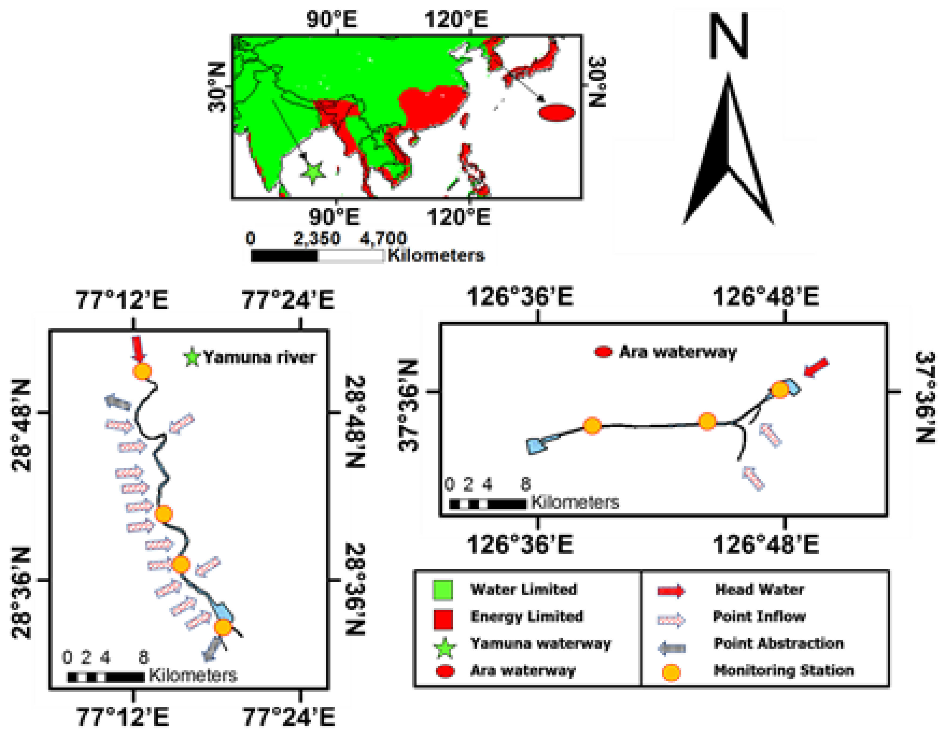
The study was conducted over energy limited and water limited regions on the basis of the global climatological aridity index (GCAI). Regions were separated using global data assimilation system (GLDAS) datasets conferring to the concept of a framework known as Budyko [34,35]. The GCAI is a numerical indicator of the degree of dryness or wetness (GCAI = PTm/Pm, where PTm = mean annual potential evapotranspiration and Pm = mean annual precipitation). The regions having an index value GCAI < 1.5 were classified as “energy limited”, and those with GCAI > 1.5 as “water limited” [36]. Two Waterways were selected, one from the energy limited regions: Gyeongin Ara Waterway also known as Ara Canal, South Korea, and the other from the water limited region: Yamuna River, India. Figure 1 shows a description of the study area, Waterways, and point source locations.
2.1.1. The Gyeongin Ara Waterway
The Gyeongin Ara Waterway is a recently constructed canal in South Korea. The main source of the flow in the Ara Waterway is the naturally sourced water from the Han River and the Gulpocheon River. The Ara Waterway was built to control flood indemnities in the basin of the Gulpocheon River and also to encourage the socio-economic growth of the area by reducing logistic expenses. The Waterway connects the Han River to the Yellow Sea. The Han River passes through Seoul and the western coastline zone of South Korea. There are two operation gates at both ends of the Waterway. The Han River side has a canal gate which is situated beside the Haengju bridge downstream of the Han River, while the Yellow Sea side has another gate that is situated at the Incheon city beside the western coastline zone of South Korea. The Ara Waterway has an overall length of about 19 km, while the width of the Waterway channel is about 85 m, and the mean depth of flowing water is 6.3 m. The head water inflow is discharged directly into the Waterway from the Han River, while there are other point sources, including water inflow from the Gulpocheon River, the irrigation dam, and the Rubber dam especially, during flood seasons.
2.1.2. The Yamuna River
The Yamuna Waterway, also primarily known as the Yamuna River, is the main source of domestic supply for New Delhi, India. It receives a huge volume of pollution in the stretch between New Delhi and Agra. From Palla, it travels about 10 km to Waziarabd, where the river’s water is drained to the greatest extent possible for the city of New Delhi’s domestic use. Thereafter, a small quantity of river water is observed, especially during the summer seasons.
After the Wazirabad barrage, a major drain known as the Najafghar drain enters the river. However, after the Najafghar drain, there are a total of thirteen small- to medium-sized drains that join the Yamuna River downstream. Approximately 39 km downstream of Palla, the river departs the city near the Okhla Barrage. The Yamuna basin has a total area of 9500 hectares, of which 8000 hectares are direct runoff [36]. Point sources, which discharge contaminated materials directly into the Yamuna River, are the most significant sources of Yamuna water pollution.
2.2. Data Set
This study used three different types of data sets, GLDAS 2.1 data, point source inflow, the initial con-centration of water quality variables, and Landsat 8 satellite data. The GLDAS (global land data assimilation system) datasets have been prepared through the collaboration of the following international agencies: NOAA, NASA, GSFC, and the NCEP. The GLDAS simulated datasets were developed to deliver medium resolution datasets by assimilating satellite-based and ground-based measurements involving the land surface models and data integration methods. Numerous land surface models have been created for the simulation of water and energy flux transferences among the ground and atmosphere interactions [37]. The water quality modelling data included point discharge, point source pollutant loadings of BOD, DO, T-N, river hydraulics characteristics data, and environmental parameters used in model simulations as the annual and seasonal bases for the year 2014. The water quality and river hydraulic characteristics data for the Yuma River, India, were obtained from various government and private agencies such as the Ministry of Environment, Upper Yamuna River Board, India River Forum, and Central Pollution Control Board. While the Water quality and hydraulic characteristics data of Ara Waterway, Republic of Korea were obtained from different Korean water and environment agencies such as the Ministry of Environment Korea, KWater, ECOREA, the national ATLAS of Korea, and Water and Environment Partnership in Asia (WEPA). The Landsat 8 satellite, cloud free images from Operational Land Imager (OLI) level-1 were utilized for the calculations of the vegetation index in all four seasons for the year 2014.
2.3. Water Quality Modeling
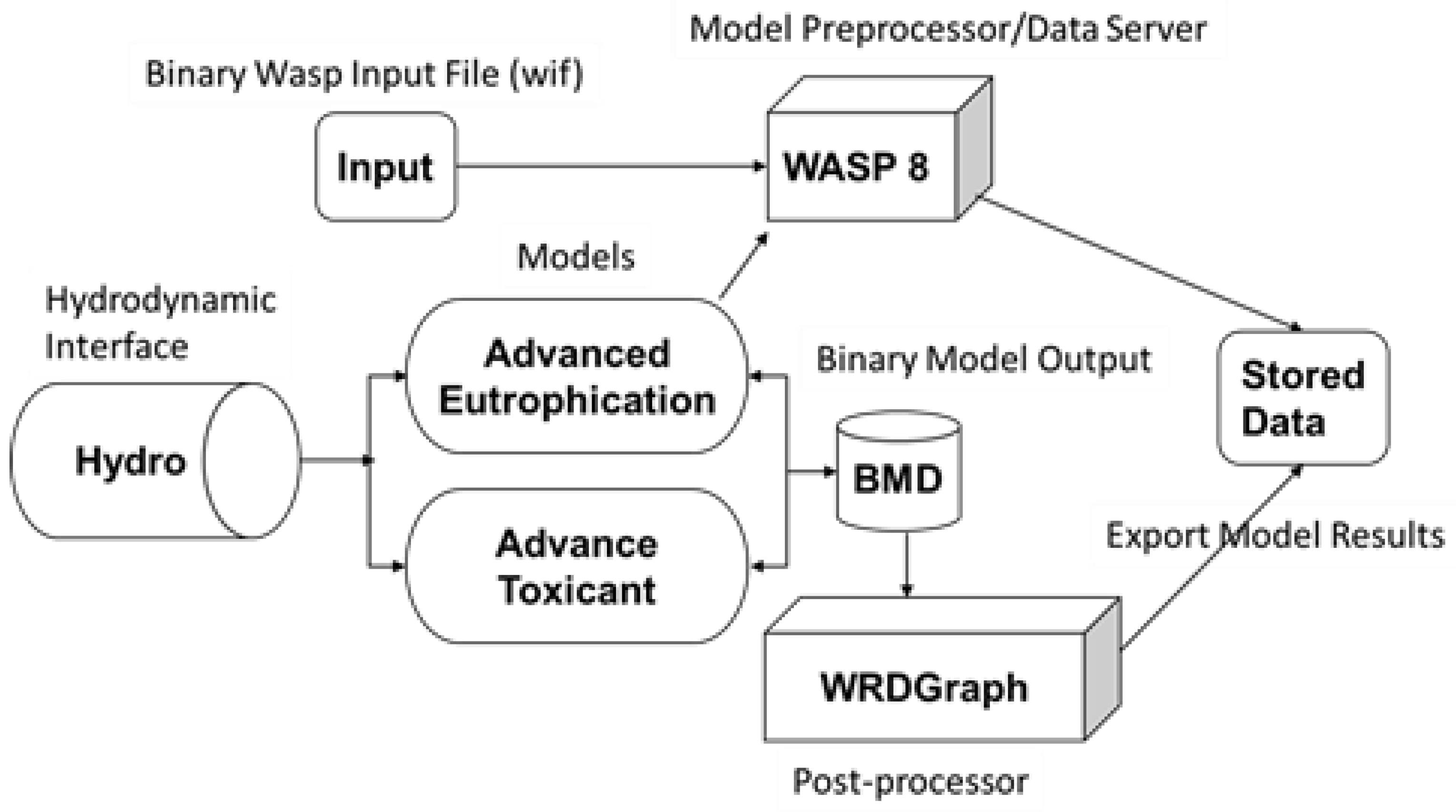
The US Environmental Protection Agency (EPA) has developed the WASP model for resolving issues of water quality. The WASP model has been continually developed over the years, allowing for greater simplicity of use and superior modelling of water quality in a wide range of water environments [24,38,39]. The WASP model is a water column and sediment-based dynamic simulation software for rivers and ponds. Toxicant transformation and advanced eutrophication are two kinetic modules in the WASP8 model employed in this investigation. One of the most complex modules, the advanced eutrophication module, incorporates many eutrophication characteristics. Many mass balance equations are included in this module to calculate the fate, transformations, phytoplankton, BOD, DO, and nitrification dynamics of pollution. This diagram shows the WASP8 model’s interconnections, features, and structure (Figure 2). In order to calculate any parameters of water quality, the equation of mass balance is utilized, which is represented in Equation (1).
Whereas C represents the concentration of different parameters of water quality factors, U represents the average water velocity, A represents the cross-sectional area, and x represents the distance in one dimension. SC stands for exterior and internal sinks and sources, whereas E stands for longitudinal dispersion coefficient.
The model was developed using the required hydraulics and the water quality datasets from 2014 to 2015. The Ara Waterway longitudinal profile was equally divided into 23 segments, containing headwater inflow from the Han River and two other inflow sources from the irrigation dam and the rubber dam. The Yamuna Waterway longitudinal profile was divided into 34 segments. The inflow drains include Najafghar, Khyber Pass, Drain No 14, Magazine Road, Metcalf House, Sweeper Colony, Mori Gate, Tonga Stand, Sen Nursing, Civil Military Drain, Drain No 14, Barapulla, Power House, Maharani Bagh Drain, Hindon Cut, and the Agra Canal Abstraction. Boundaries, which included the most upstream segments of the Ara Waterway (segments 1 to 23), while the Yamuna Waterway includes point source inflow and obstructions throughout the Waterway longitudinal profile (segments 1 to 34), and was added as an initial concentration to the simulation for all the water quality variables.
2.4. Vegetation Indices
The vegetation indices are spectral transformations of two or more spectral bands combined to improve the involvement of plant properties, permit appropriate space time scale inter and intra-comparisons of global photosynthetic activities and vegetation structure distinctions. In this study, we calculated vegetation index, entitled normalized difference vegetation index (NDVI). A commonly applied vegetation index, the NDVI has long been used in ecology, remote sensing, and geography to assess the characteristics of green vegetation, including its amount (biomass), nature, and status. NDVI is a benchmark for spectral band ratio applications [40]. The NDVI monitors the vegetation state, density, and intensity of plant growth, and can be calculated from the reflectance values of the red (RED) and the infrared band (NIR). The NDVI values range from −1.0 to +1.0, lower values indicating sparse vegetation while higher values indicate lush green land. The NDVI was obtained from the reflectance values of Landsat 8 scenes by means of ArcGIS. Prepossessing of Landsat 8 scenes was performed using ENVI 5.2 software and metadata information. The following equation used to calculate the NDVI values was expressed as Equation (2):
2.5. Model Accuracy Assesment
The model’s accuracy was assessed by contrasting the actual results with those predicted by the model. It was determined that the calibrated and validated results from the prior experiments were accurate using the following five statistical estimators:
Goodness-of-fit between observed and expected data can be measured using the coefficient of determination (R2). The R2 has a value of 0 to 1. If R2 is near to 1, then the model’s predictions match the actual data quite well.
When comparing observed and expected results, the MAE assesses the absolute quantitative deviation. The formula for MAE is as follows:
An index known as the mean absolute percentage error (MAPE) was calculated to appraise the precision of the modelled outputs. The fewer the errors, the closer the fittings of the modelled results [41], which were defined as four different stages of fitting levels, each conferring to model evaluations such as excellent, good, reasonable, and poor. If MAPE value <10%, fitting level is excellent, if MAPE value is 10–20%, fitting level is good, if MAPE value: 20–50%, fitting level is reasonable, and if MAPE value >50%, fitting level is poor.
Here, S is a modeled outcome for a similar profile place where field observations were made for calibration and validation processes, and O is the observed value obtained from the mainstream sampling point. The total number of all the measurements were represented by N, and i is ith comparison. An observational average and a model-based simulation average are used to calculate O and S, respectively, for each location.
3. Results
3.1. Evaluation of the WASP8 Model for Its Reliability
Assessment of the WASP8 consists of a model calibration and validation investigation to establish its applicability for involvement analysis.
The WASP8 Calibrations and Validations
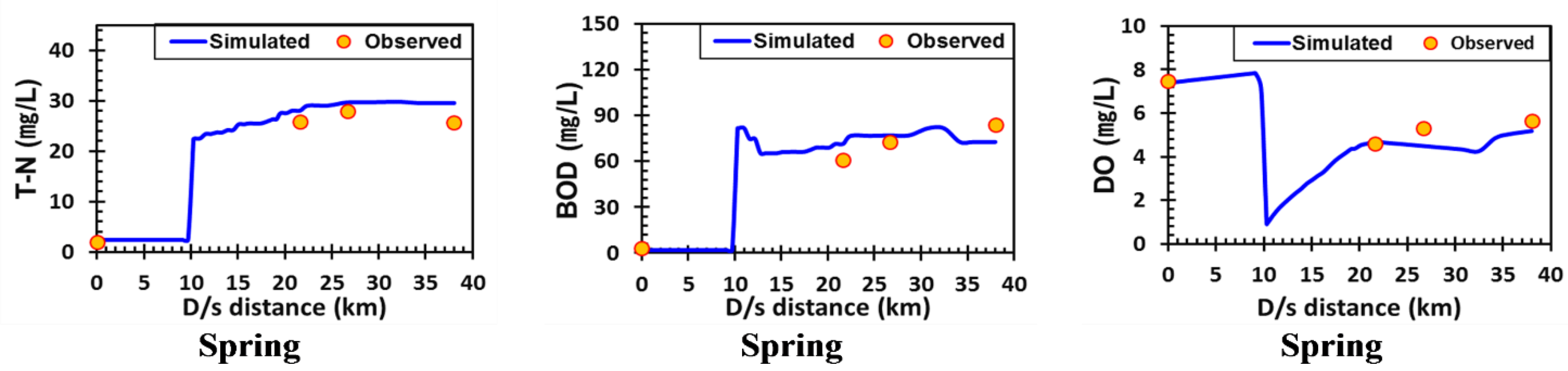
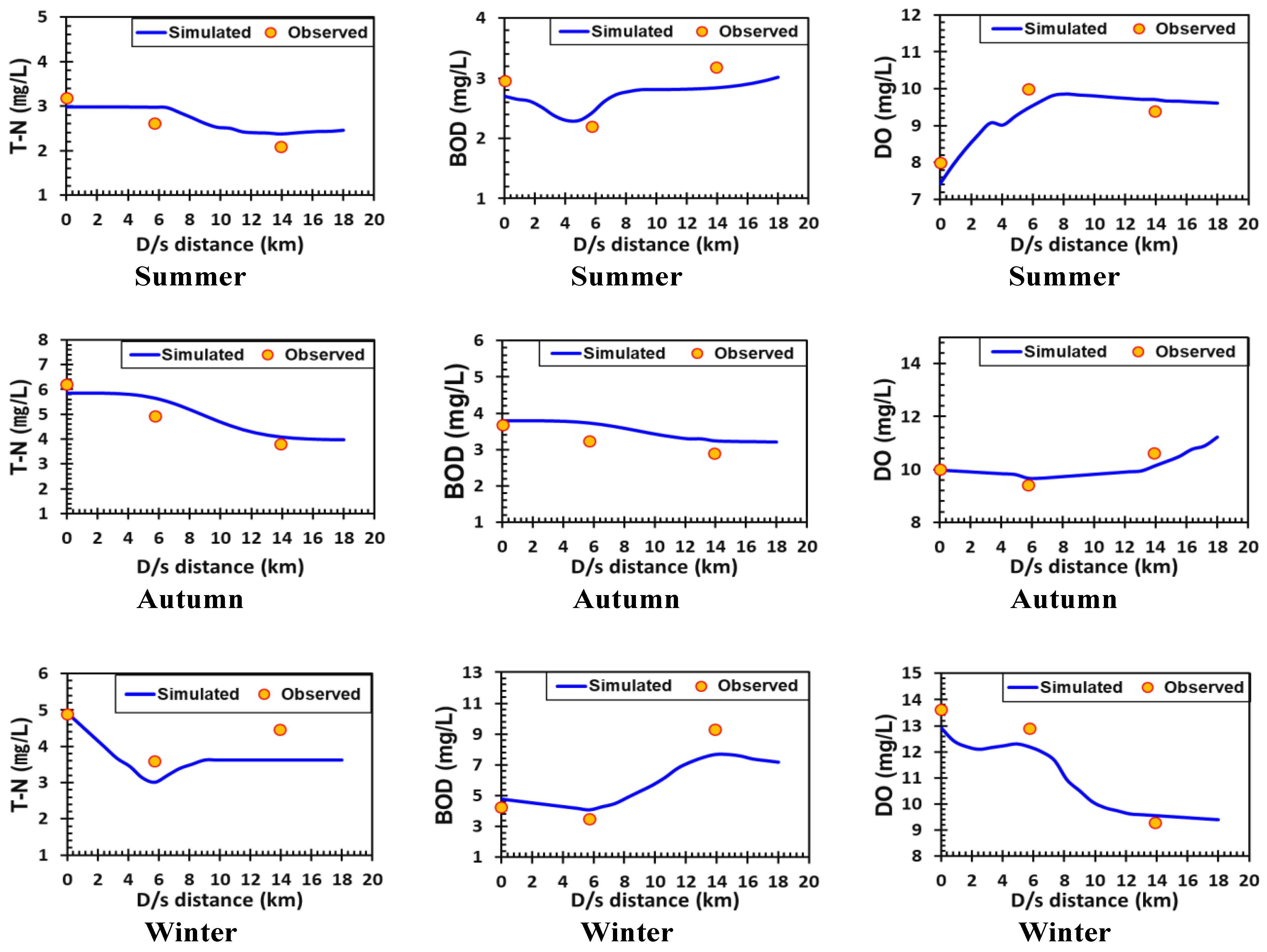
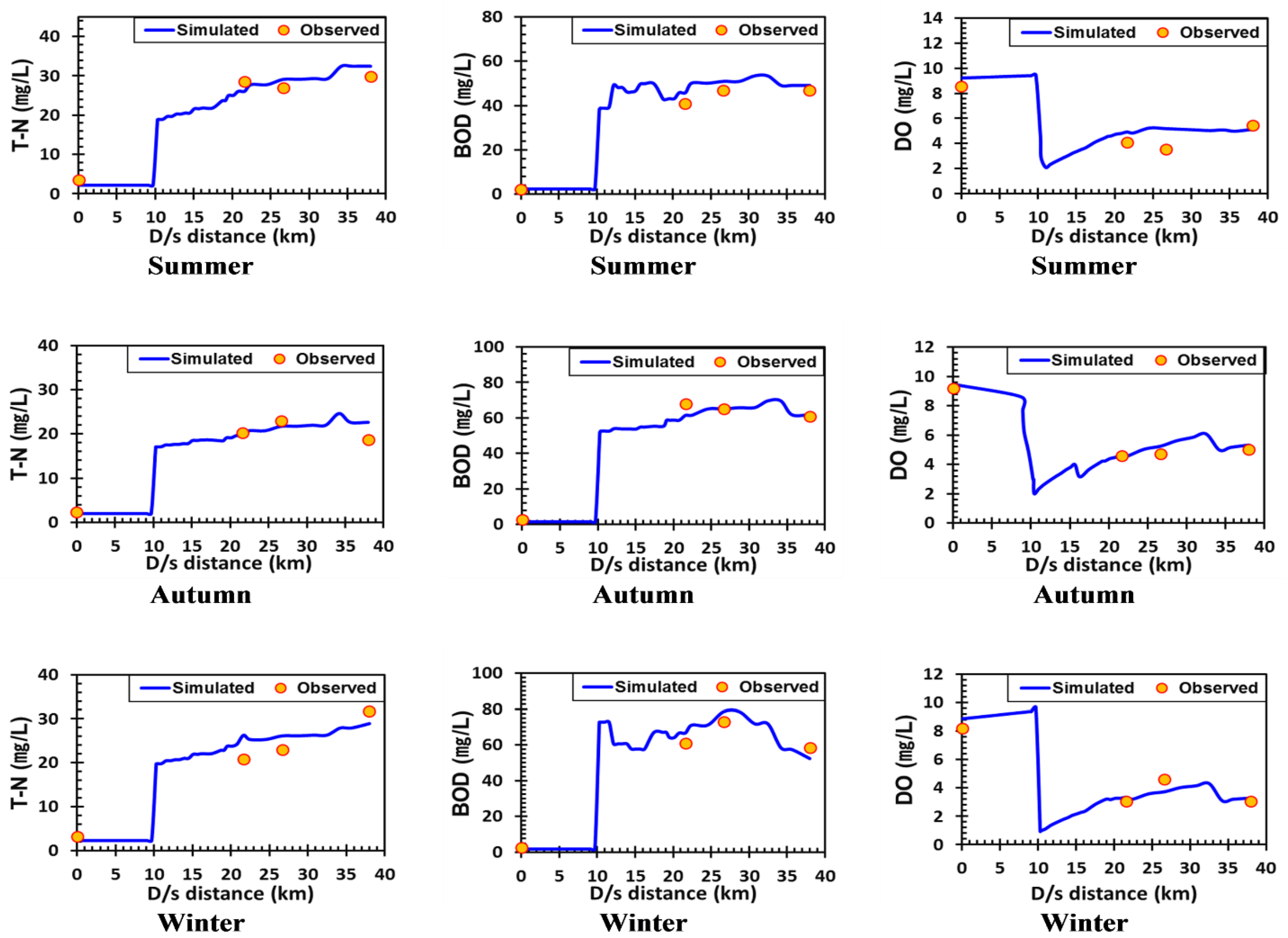
The surface water quality model WASP8 was primarily calibrated through the measured data attained from the four sampling locations (M1–M4) along the longitudinal stream of the Yamuna river and three sampling stations of the Ara Canal (m1–m3) Waterway on March, 2014 (spring) using the same measured coefficients (Figure 3 and Figure 4). Then, the data collected from June (summer), September (autumn) and December (winter) were used to validate the model also by means of the same estimated reaction constants and model coefficients (Figure 5 and Figure 6). Calibrated and validated results of the longitudinal pro-file of T-N, BOD, and DO, agreeing well with the measured values at monitoring stations and both measured and simulated, had the analogous trend of variations. The Ara Waterway shows comparatively large seasonal variation, which might be due to higher mean annual rainfall in the wetter region [42].
The mean absolute percentage error (MAPE) evaluation shows that the values were enclosed among 3.5–22.61% (excellent–reasonable) (Table 1). The mean absolute error (MAE) shows overall estimator errors are less and agreed well with the measured data both in model calibration and validation processes (Table 2). The values of coefficient of determination R2 had good agreement with measured data and appeared to be very close to 1 (Table 3). Moreover, all applied statistical estimators show high value of R2 (close to 1) and lower values of errors of estimators. Overall, longitudinal profile of Yamuna Waterway shows small seasonal variation among water quality variables. At the headwater, water quality was comparatively better. However, after addition of point inflow through Najaf-garh drain water quality was further deteriorated. While, Ara Waterway showed large noticeable variation in water quality variables among each season. Total nitrogen shows a decreasing trend as it moves toward a downstream end in all seasons, while BOD and DO show further deterioration in water quality as they go toward a downstream end of the waterway profile in winter and summer seasons. In spring and autumn, BOD and DO both show improvement in water quality profile as higher rate fresh water point inflow is incorporated in waterways.
3.2. Spatial Scale Interrelationship between the Water Quality and Vegetation Indices
In the following study, we calculated vegetation index of both the Yamuna and the Ara Waterway basins at an annual and seasonal scale for the year 2014. For the case of the Ara Waterway, the vegetations are distributed sparsely along the coastline region, the Yellow Sea, while, the Yamuna Waterway has a dense vegetation beside the upstream and downstream regions. The NDVI values around −0.26 or less depicts a water body, values near −0.046 show snow, values near 0.002 show clouds, values near 0.025 show bare soil and values greater than 0.6 show dense vegetation. Table 4 shows the interrelationship among the vegetation index and water quality variables during the different seasons. At an annual and seasonal scale, both waterways showed higher interrelationship among vegetation index, T-N and BOD.
However, vegetation cover has negative and the lower correlation coefficient values with DO. Overall, the water quality of the Ara Waterway has a higher correlation coefficient value than the Yamuna Waterway. From these results, we can interpret that there is some relationship between river water quality and vegetation bio-mass, and the relationship is stronger when it comes to the case of the wetter region. So, the vegetation results in more effects on stream water quality located in wetter regions.
Over basic relationships between vegetation and random point data, the use of long-term profiles provides advantages over the use of point-based water quality data. The vegetation index values take into account all green vegetation. NDVI values, for example, illustrate the effect of grassland, as well as agricultural and residential land values in a largely vegetated area. These values may be more or less associated with environmental conditions as a whole than they would be individually.
The NDVI value can, however, indicate the health of crop vegetation at various phonological growth stages, including lowered status or enhanced vegetation in a farming watershed, which may be a result of fertilizer use. Alternatively, one can examine the physical link between quality of water and a vegetation index by analyzing a regulated set of water quality and the average value of nearby vegetation indexes. Although other factors affecting the water quality include increased vegetation, greenness and moistness are related to the activities of plant physiology. Water consumption and enhanced nutrient uptake, such as oxygen and nitrogen demand, could be linked to the vegetated area, which may result in even less chemicals entering the water stream via non-point source linkage. In order to discover the root reason of the correlation between quality of water and vegetation indicators, more research is needed.
3.3. Study Limitation
In the following study, we tried to illustrate the importance of seasonal and regional based water quality management and a connection with vegetation and stream water quality. Understanding the variability in vegetation index values, of course, will depend on the mixture of different vegetation types. Because higher values of vegetation indices are not necessarily the only reason for higher interrelationship, water quality might also be affected with several degrees to different types of vegetation such as riverside forest or bushes.
Human errors introduced in this study might include errors in river boundary and general errors in the WASP modelling development. Any small variation in the segment length and vegetation index area of interest could result in a large percentage error in setting the interrelationship between the water quality and vegetation indices. In some cases, no equal number of Landsat 8 cloud free scenes is available in each season for vege-tation index acquisition. However, the study applied the average of all the available image indices for each season, and then a similar methodology was also performed with the water quality data for model simulation.
More than only vegetation biomass may have contributed to stream pollution, as evidenced by the lower R2 values observed. Types of vegetation, land cover, soils, and other contaminant sources are all examples of these elements in play. It is possible to gain insight into the factors affecting the relations of interest by performing this type of interrelationship analysis. Future research that incorporates extensive water quality modelling with a variety of vegetation assessments and land cover classifications could be helpful in addressing this issue.
The outcomes presented in the following study showed an interrelationship among the water quality and the vegetation indices, which revealed that there must be a connection between the green vegetation biomass and the stream water quality. Furthermore, in the spring season, correlations were highest for the case of total nitrogen and biochemical oxygen demand due to the presence of higher vegetation [30]. This study also supports the theories of [31], who hypothesized that vegetation indices have the potential to some extent in illustrating stream water quality. This work is the first of its kind to use advanced water quality modelling to show how plant indices and stream water quality are linked at the spatial scale of river segments. Furthermore, this is also the first time that geographical regions were divided into a wetter and a drier region on the basis of the global climatological aridity index to investigate in a broad context.
4. Conclusions
Stream water quality was predicted using the WASP8 model in this study, which was applied to the longitudinal profile of both waterways. The modelling results were appraised through the assessment of fitting levels with MAPE analysis over both average and seasonal scales. The results showed a large temporal variation of the water quality concentration among seasonal scale in the Ara Waterway, which comes in the wet region, while in the dry region Yamuna Waterway showed small-scale seasonal variation in a longitudinal profile of the river water quality. Furthermore, an interrelationship was investigated among vegetation indices and water quality variables.
The Ara Waterway, which comes in wetter regions, showed relatively better connection between water quality variables and vegetation indices on the annual scale for T-N, BOD and DO with Pearson correlation coefficient values at about 0.66, 0.68 and −0.58, respectively. The seasonal scale interrelationship between water quality and NDVI also showed strong linkage in the energy limited region over the Ara Waterway than that of the water limited region, with a maximum correlation coefficient value occur in the spring season.
The seasonal variation of water quality variables over different geological locations will help us to understand the water quality management over different climatic regions. The management of water quality dynamics and its relationship with vegetation indices over different climatological regions will help us in monitoring and managing water quality with different strategy levels. The results of this research are advantageous for water quality management and waterway restoration, as they highlight the effects of vegetation and the relationship between water quality and vegetation indices. The variance in water quality may vary with the variation in season and vegetation biomass. Thus, better water quality of sustainable water environment could be achieved by making management strategies conferring to the different geographical region’s specific vegetation patterns.
Author Contributions
Conceptualization, M.M.I., J.L.L. and S.H.; methodology, M.M.I., S.H., J.L.L., M.S.W.; software, M.M.I., S.H., J.L.L.; validation, M.M.I., S.H., J.L.L., A.D., A.E. and F.M.; formal analysis, M.M.I., M.S.W. and S.H.; investigation, M.M.I. and S.H.; resources, M.M.I., S.H., M.S.W., F.M., A.E. and L.L.; data curation, M.M.I. and S.H.; writing—original draft preparation, M.M.I. and S.H.; writing—review and editing, M.M.I., S.H., J.L.L., F.M., A.E., A.D., L.L.; visualization, M.M.I., F.M., A.D., A.E., L.L.; supervision, J.L.L., L.L.; project administration, M.M.I., S.H., M.S.W., L.L.; funding acquisition, J.L.L., S.H., L.L. All authors have read and agreed to the published version of the manuscript.
Funding
The funding is provided by the Civil Aerospace Technology Advance Research. (Grant No. Y7K00100KJ).
Institutional Review Board Statement
Not applicable.
Informed Consent Statement
Not applicable.
Data Availability Statement
Not applicable.
Acknowledgments
The authors are thankful to the Coastal and Environmental Laboratory, Graduate School of Water Resources, Sungkyunkwan University for providing resources and funding for designed research. The first and second author was supported through a scholarship funding’s by the Higher Education Commission, Pakistan.
Conflicts of Interest
The authors declare no conflict of interest.
References
- van Vliet, M.T.; Jones, E.R.; Flörke, M.; Franssen, W.H.; Hanasaki, N.; Wada, Y.; Yearsley, J.R. Global water scarcity including surface water quality and expansions of clean water technologies. Environ. Res. Lett. 2021, 16, 024020. [Google Scholar] [CrossRef]
- Schwarzenbach, R.P.; Egli, T.; Hofstetter, T.B.; Von Gunten, U.; Wehrli, B. Global water pollution and human health. Annu. Rev. Environ. Resour. 2010, 35, 109–136. [Google Scholar] [CrossRef]
- Choque-Quispe, D.; Froehner, S.; Palomino-Rincón, H.; Peralta-Guevara, D.E.; Barboza-Palomino, G.I.; Kari-Ferro, A.; Zamalloa-Puma, L.M.; Mojo-Quisani, A.; Barboza-Palomino, E.E.; Zamalloa-Puma, M.M. Proposal of a Water-Quality Index for High Andean Basins: Application to the Chumbao River, Andahuaylas, Peru. Water 2022, 14, 654. [Google Scholar] [CrossRef]
- Alexakis, D.; Gotsis, D.; Giakoumakis, S. Assessment of drainage water quality in pre-and post-irrigation seasons for supplemental irrigation use. Environ. Monit. Assess. 2012, 184, 5051–5063. [Google Scholar] [CrossRef] [PubMed]
- Arora, S.; Keshari, A.K. Dissolved oxygen modelling of the Yamuna River using different ANFIS models. Water Sci. Technol. 2021, 84, 3359–3371. [Google Scholar] [CrossRef] [PubMed]
- Zahraeifard, V.; Deng, Z. VART model–based method for estimation of instream dissolved oxygen and reaeration coefficient. J. Environ. Eng. 2012, 138, 518–524. [Google Scholar] [CrossRef]
- Park, S.S.; Lee, Y.S. A water quality modeling study of the Nakdong River, Korea. Ecol. Model. 2002, 152, 65–75. [Google Scholar] [CrossRef]
- Iqbal, M.M.; Shoaib, M.; Agwanda, P.; Lee, J.L. Modeling approach for water-quality management to control pollution concentration: A case study of Ravi River, Punjab, Pakistan. Water 2018, 10, 1068. [Google Scholar] [CrossRef] [Green Version]
- Khan, R.; Inam, M.A.; Iqbal, M.M.; Shoaib, M.; Park, D.R.; Lee, K.H.; Shin, S.; Khan, S.; Yeom, I.T. Removal of ZnO nanoparticles from natural waters by coagulation-flocculation process: Influence of surfactant type on aggregation, dissolution and colloidal stability. Sustainability 2019, 11, 17. [Google Scholar] [CrossRef] [Green Version]
- Iqbal, M.M.; Shoaib, M.; Farid, H.U.; Lee, J.L. Assessment of water quality profile using numerical modeling approach in major climate classes of Asia. Int. J. Environ. Res. Public Health 2018, 15, 2258. [Google Scholar] [CrossRef] [Green Version]
- Liu, B.; Dong, D.; Hua, X.; Dong, W.; Li, M. Spatial Distribution and Ecological Risk Assessment of Heavy Metals in Surface Sediment of Songhua River, Northeast China. Chin. Geogr. Sci. 2021, 31, 223–233. [Google Scholar] [CrossRef]
- Huang, L.; Bai, J.; Xiao, R.; Gao, H.; Liu, P. Spatial distribution of Fe, Cu, Mn in the surface water system and their effects on wetland vegetation in the Pearl River Estuary of China. CLEAN–Soil Air Water 2012, 40, 1085–1092. [Google Scholar] [CrossRef]
- Wang, Q.; Li, S.; Jia, P.; Qi, C.; Ding, F. A review of surface water quality models. Sci. World J. 2013, 2013, 231768. [Google Scholar] [CrossRef] [PubMed] [Green Version]
- Farid, H.U.; Ahmad, I.; Anjum, M.N.; Khan, Z.M.; Iqbal, M.M.; Shakoor, A.; Mubeen, M. Assessing seasonal and long-term changes in groundwater quality due to over-abstraction using geostatistical techniques. Environ. Earth Sci. 2019, 78, 386. [Google Scholar] [CrossRef]
- Ali, A.; Iqbal, M.; Khattak, K.K. Pilot plant investigation on the start-up of a UASB reactor using sugar mill effluent. Cent. Asian J. Environ. Sci. Technol. Innov. 2020, 1, 199–205. [Google Scholar]
- Cox, B. A review of currently available in-stream water-quality models and their applicability for simulating dissolved oxygen in lowland rivers. Sci. Total Environ. 2003, 314, 335–377. [Google Scholar] [CrossRef]
- Iqbal, M.M.; Shoaib, M.; Agwanda, P.O. The response of pollution load from coastal river waterfront on red tides in South Sea. J. Coast. Res. 2019, 91, 231–235. [Google Scholar] [CrossRef]
- Fan, C.; Ko, C.-H.; Wang, W.-S. An innovative modeling approach using Qual2K and HEC-RAS integration to assess the impact of tidal effect on River Water quality simulation. J. Environ. Manag. 2009, 90, 1824–1832. [Google Scholar] [CrossRef]
- Morley, N.J. Anthropogenic effects of reservoir construction on the parasite fauna of aquatic wildlife. EcoHealth 2007, 4, 374–383. [Google Scholar] [CrossRef]
- Shoaib, M.; Iqbal, M.M.; Khan, R.; Lee, J.L. An Analytical Study for Eutrophication Management of Arawaterway, Korea, by Developing a Flow Model. J. Coast. Res. 2019, 91, 226–230. [Google Scholar] [CrossRef]
- Agwanda, P.O.; Iqbal, M.M. Engineering Control of Eutrophication: Potential Impact Assessment of Wastewater Treatment Plants Around Winam Gulf of Lake Victoria in Kenya. J. Coast. Res. 2019, 91, 221–225. [Google Scholar] [CrossRef]
- Kannel, P.R.; Kanel, S.R.; Lee, S.; Lee, Y.-S.; Gan, T.Y. A review of public domain water quality models for simulating dissolved oxygen in rivers and streams. Environ. Modeling Assess. 2011, 16, 183–204. [Google Scholar] [CrossRef]
- Yang, C.-P.; Kuo, J.-T.; Lung, W.-S.; Lai, J.-S.; Wu, J.-T. Water quality and ecosystem modeling of tidal wetlands. J. Environ. Eng. 2007, 133, 711–721. [Google Scholar] [CrossRef]
- Ambrose, R.B.; Wool, T.A.; Martin, J.L. The Water Quality Analysis Simulation Program, WASP5, Part A: Model Documentation; Environmental Research Laboratory, US Environmental Protection Agency: Athens, GA, USA, 1993.
- Alam, A.; Badruzzaman, A.; Ali, M.A. Assessing effect of climate change on the water quality of the Sitalakhya river using WASP model. J. Civ. Eng. 2013, 41, 21–30. [Google Scholar]
- Akomeah, E.; Chun, K.P.; Lindenschmidt, K.-E. Dynamic water quality modelling and uncertainty analysis of phytoplankton and nutrient cycles for the upper South Saskatchewan River. Environ. Sci. Pollut. Res. 2015, 22, 18239–18251. [Google Scholar] [CrossRef] [PubMed]
- Chen, C.-Y.; Tien, C.-J.; Sun, Y.-M.; Hsieh, C.-Y.; Lee, C.-C. Influence of water quality parameters on occurrence of polybrominated diphenyl ether in sediment and sediment to biota accumulation. Chemosphere 2013, 90, 2420–2427. [Google Scholar] [CrossRef] [PubMed]
- Yang, C.-P.; Lung, W.-S.; Kuo, J.-T.; Lai, J.-S.; Wang, Y.-M.; Hsu, C.-H. Using an integrated model to track the fate and transport of suspended solids and heavy metals in the tidal wetlands. Int. J. Sediment Res. 2012, 27, 201–212. [Google Scholar] [CrossRef]
- Nazeer, S.; Hashmi, M.Z.; Malik, R.N. Heavy metals distribution, risk assessment and water quality characterization by water quality index of the River Soan, Pakistan. Ecol. Indic. 2014, 43, 262–270. [Google Scholar] [CrossRef]
- Tang, P.-K.; Huang, Y.-C.; Kuo, W.-C.; Chen, S.-J. Variations of model performance between QUAL2K and WASP on a river with high ammonia and organic matters. Desalin. Water Treat. 2014, 52, 1193–1201. [Google Scholar] [CrossRef]
- Xue, J.; Su, B. Significant remote sensing vegetation indices: A review of developments and applications. J. Sens. 2017, 2017, 1353691. [Google Scholar] [CrossRef] [Green Version]
- Hussain, S.; Masud Cheema, M.J.; Arshad, M.; Ahmad, A.; Latif, M.A.; Ashraf, S.; Ahmad, S. Spray uniformity testing of unmanned aerial spraying system for precise agro-chemical applications. Pak. J. Agric. Sci. 2019, 56, 897–903. [Google Scholar]
- Dosskey, M.G.; Vidon, P.; Gurwick, N.P.; Allan, C.J.; Duval, T.P.; Lowrance, R. The role of riparian vegetation in protecting and improving chemical water quality in streams 1. JAWRA J. Am. Water Resour. Assoc. 2010, 46, 261–277. [Google Scholar] [CrossRef]
- Donohue, R.; Roderick, M.; McVicar, T.R. On the importance of including vegetation dynamics in Budyko’s hydrological model. Hydrol. Earth Syst. Sci. 2007, 11, 983–995. [Google Scholar] [CrossRef] [Green Version]
- Li, D.; Pan, M.; Cong, Z.; Zhang, L.; Wood, E. Vegetation control on water and energy balance within the Budyko framework. Water Resour. Res. 2013, 49, 969–976. [Google Scholar] [CrossRef]
- Zhang, Y.; Leuning, R.; Chiew, F.H.; Wang, E.; Zhang, L.; Liu, C.; Sun, F.; Peel, M.C.; Shen, Y.; Jung, M. Decadal trends in evaporation from global energy and water balances. J. Hydrometeorol. 2012, 13, 379–391. [Google Scholar] [CrossRef]
- Rodell, M.; Houser, P.; Jambor, U.; Gottschalck, J.; Mitchell, K.; Meng, C.-J.; Arsenault, K.; Cosgrove, B.; Radakovich, J.; Bosilovich, M. The global land data assimilation system. Bull. Am. Meteorol. Soc. 2004, 85, 381–394. [Google Scholar] [CrossRef] [Green Version]
- Ambrose, B.; Wool, T.; Martin, J. The Water Quality Analysis Simulation Program, WASP6, User Manua; US EPA: Athens, GA, USA, 2001. [Google Scholar]
- Hao, L.; Cheng, L.; Bi, X. Apply with WASP Water Quality Model. In Proceedings of the the 2nd International Conference on Computer Application and System Modeling; Atlantis Press: Paris, France, 2012; pp. 714–717. [Google Scholar]
- Filippova, N.V.; Bulyonkova, T.M.; Lapshina, E. Fleshy fungi forays in the vicinities of the YSU Mukhrino field station. Environ. Dyn. Glob. Clim. Chang. 2015, 6, 3–31. [Google Scholar] [CrossRef] [Green Version]
- Joyce, D.; Joyce, L.; Locke, M. Mechanical Circulatory Support: Principles and Applications; McGraw-Hill Education/Medical: New York, NY, USA, 2011. [Google Scholar]
- Yeon, Y.J.; Kim, D.H.; Lee, J.L. Water quality modeling for integrated management of urban stream networks. Int. J. Environ. Sci. Dev. 2016, 7, 928. [Google Scholar] [CrossRef] [Green Version]
Figure 1.
Study area description.

Figure 2.
Components and the assembly of WASP8 model.

Figure 3.
Calibration of water qualities in the Ara Waterway for the Spring season.

Figure 4.
Calibration of water qualities in the Yamuna Waterway for the spring season.

Figure 5.
Confirmation of water qualities in the Ara Waterway for summer, autumn, and winter seasons.
Figure 5.
Confirmation of water qualities in the Ara Waterway for summer, autumn, and winter seasons.

Figure 6.
Confirmation of water qualities in the Yamuna Waterway for summer, autumn, and winter seasons.
Figure 6.
Confirmation of water qualities in the Yamuna Waterway for summer, autumn, and winter seasons.


Table 1.
Fitting level assessment of the WASP8 outcomes with MAPE process.
| River | Season | T-N (%) | BOD (%) | DO (%) | |||
|---|---|---|---|---|---|---|---|
| Calibration | Validation | Calibration | Validation | Calibration | Validation | ||
| Yumna River | Spring | 17.07 | 16.25 | 10.22 | 9.14 | 8.11 | 9.21 |
| Summer | 10.37 | 9.36 | 8.33 | 8.43 | 6.34 | 6.56 | |
| Autumn | 7.54 | 8.34 | 6.91 | 7.25 | 6.08 | 6.73 | |
| Winter | 14.67 | 16.32 | 15.5 | 13.94 | 6.62 | 6.94 | |
| Ara Water Way | Spring | 22.61 | 22.24 | 7.55 | 8.92 | 15.34 | 16.31 |
| Summer | 9.70 | 9.56 | 5.75 | 4.95 | 8.53 | 8.94 | |
| Autumn | 12.4 | 13.1 | 3.50 | 4.31 | 7.41 | 7.64 | |
| Winter | 16.71 | 15.93 | 7.73 | 6.72 | 11.79 | 12.45 | |
| MAPE value, excellent; <10%, good; 10–20%, reasonable; 20–50%, bad; >50% | |||||||
Table 2.
Fitting level assessment of the WASP8 outcomes with MAE estimator.
| River | Season | T-N (%) | BOD (%) | DO (%) | |||
|---|---|---|---|---|---|---|---|
| Calibration | Validation | Calibration | Validation | Calibration | Validation | ||
| Yumna River | Spring | 0.15 | 0.16 | 0.62 | 0.58 | 0.12 | 0.13 |
| Summer | 0.11 | 0.12 | 0.35 | 0.27 | 0.08 | 0.07 | |
| Autumn | 0.09 | 0.11 | 0.31 | 0.35 | 0.06 | 0.08 | |
| Winter | 0.17 | 0.15 | 0.78 | 0.66 | 0.14 | 0.12 | |
| Ara Water Way | Spring | 0.13 | 0.14 | 0.44 | 0.51 | 0.10 | 0.11 |
| Summer | 0.09 | 0.11 | 0.29 | 0.25 | 0.06 | 0.07 | |
| Autumn | 0.11 | 0.11 | 0.31 | 0.28 | 0.08 | 0.08 | |
| Winter | 0.16 | 0.14 | 0.52 | 0.47 | 0.13 | 0.11 | |
Table 3.
Fitting level assessment of the WASP8 outcomes with R2 estimator.
| River | Season | T-N (%) | BOD (%) | DO (%) | |||
|---|---|---|---|---|---|---|---|
| Calibration | Validation | Calibration | Validation | Calibration | Validation | ||
| Yumna River | Spring | 0.81 | 0.84 | 0.85 | 0.88 | 0.87 | 0.84 |
| Summer | 0.89 | 0.83 | 0.88 | 0.92 | 0.87 | 0.82 | |
| Autumn | 0.88 | 0.93 | 0.90 | 0.89 | 0.93 | 0.89 | |
| Winter | 0.84 | 0.81 | 0.86 | 0.91 | 0.92 | 0.94 | |
| Ara Water Wa | Spring | 0.82 | 0.80 | 0.86 | 0.88 | 0.85 | 0.81 |
| Summer | 0.87 | 0.94 | 0.90 | 0.89 | 0.91 | 0.88 | |
| Autumn | 0.92 | 0.96 | 0.91 | 0.88 | 0.93 | 0.91 | |
| Winter | 0.86 | 0.89 | 0.88 | 0.93 | 0.94 | 0.89 | |
Table 4.
The value of correlation coefficient among vegetation index and water quality variables.
| Stream | Period | T−N_ NDVI | BOD_ NDVI | DO_ NDVI |
|---|---|---|---|---|
| Ara | R2 | R2 | R2 | |
| Annual | 0.66 | 0.68 | −0.58 | |
| Spring | 0.69 | 0.68 | −0.59 | |
| Summer | 0.52 | 0.62 | −0.57 | |
| Autumn | 0.62 | 0.66 | −0.42 | |
| Winter | 0.42 | 0.47 | −0.39 | |
| Yamuna | Annual | 0.55 | 0.51 | −0.5 |
| Spring | 0.58 | 0.41 | −0.5 | |
| Summer | 0.42 | 0.48 | −0.4 | |
| Autumn | 0.35 | 0.44 | −0.39 | |
| Winter | 0.41 | 0.45 | −0.37 |
Publisher’s Note: MDPI stays neutral with regard to jurisdictional claims in published maps and institutional affiliations. |
© 2022 by the authors. Licensee MDPI, Basel, Switzerland. This article is an open access article distributed under the terms and conditions of the Creative Commons Attribution (CC BY) license (https://creativecommons.org/licenses/by/4.0/).
Share and Cite
MDPI and ACS Style
Iqbal, M.M.; Li, L.; Hussain, S.; Lee, J.L.; Mumtaz, F.; Elbeltagi, A.; Waqas, M.S.; Dilawar, A. Analysis of Seasonal Variations in Surface Water Quality over Wet and Dry Regions. Water 2022, 14, 1058. https://doi.org/10.3390/w14071058
AMA Style
Iqbal MM, Li L, Hussain S, Lee JL, Mumtaz F, Elbeltagi A, Waqas MS, Dilawar A. Analysis of Seasonal Variations in Surface Water Quality over Wet and Dry Regions. Water. 2022; 14(7):1058. https://doi.org/10.3390/w14071058
Chicago/Turabian StyleIqbal, Muhammad Mazhar, Lingling Li, Saddam Hussain, Jung Lyul Lee, Faisal Mumtaz, Ahmed Elbeltagi, Muhammad Sohail Waqas, and Adil Dilawar. 2022. "Analysis of Seasonal Variations in Surface Water Quality over Wet and Dry Regions" Water 14, no. 7: 1058. https://doi.org/10.3390/w14071058
Note that from the first issue of 2016, this journal uses article numbers instead of page numbers. See further details here.