Article

Enhancing Real-Time Prediction of Effluent Water Quality of Wastewater Treatment Plant Based on Improved Feedforward Neural Network Coupled with Optimization Algorithm

1
State Key Laboratory of Pollution Control and Resource Reuse, College of Environmental Science and Engineering, Tongji University, Shanghai 200092, China
2
Key Laboratory of Yangtze River Water Environment, Ministry of Education, Tongji University, Shanghai 200092, China
3
Environmental Resources, OC Public Works, County of Orange, California, 2301 North Glassell Street, Orange, CA 92865, USA
*
Author to whom correspondence should be addressed.
Water 2022, 14(7), 1053; https://doi.org/10.3390/w14071053
Submission received: 7 March 2022 / Revised: 25 March 2022 / Accepted: 25 March 2022 / Published: 27 March 2022
(This article belongs to the Section Wastewater Treatment and Reuse)

Abstract

:
To provide real-time prediction of wastewater treatment plant (WWTP) effluent water quality, a machine learning (ML) model was developed by combining an improved feedforward neural network (IFFNN) with an optimization algorithm. Data used as input variables of the IFFNN included hourly influent water quality parameters, influent flow rate and WWTP process monitoring and operational parameters. Additionally, input variables included historical effluent water quality parameters for future prediction. The model was demonstrated in a WWTP in Jiangsu Province, China, where prediction of effluent chemical oxygen demand (COD) and total nitrogen (TN) with large variations were tested. Relative to the traditional feedforward neural network (FFNN) model without considering historical effluent water quality parameter input, the IFFNN enhanced prediction performance by 52.3% (COD) and 72.6% (TN) based on the mean absolute percentage errors of test datasets, after its model structure was optimized with a genetic algorithm (GA). The problem of over-fitting could also be overcome through the use of the IFFNN, with the determination of coefficient increased from 0.20 to 0.76 for test datasets of effluent COD. The GA-IFFNN model, which was efficient in capturing complex non-linear relationships and extrapolation, could be a useful tool for real-time direction of regulatory changes in WWTP operations.

Graphical Abstract

1. Introduction

Wastewater treatment plants (WWTPs) are an important part of urban water infrastructure in pollutant reduction and public health protection. Currently WWTPs are facing increasingly stringent requirements on effluent quality, energy consumption, and resource recycling [1,2,3,4,5]. To meet these requirements, mathematical models have increasingly been employed to predict the efficiency of the WWTP and then provide suitable operation strategies, by establishing a quantitative response of WWTP influent parameters to effluent water quality.
Over the past decades, mechanistic models established with a variety of configurations for carbon, nitrogen and phosphorous removal have been the mainstream. They target either the biological processes (to achieve the treatment quality target) or various aspects of engineering (to achieve cost effective design and operation) [6,7]. Activated sludge modeling (ASM) represents an important milestone in the modeling of biological treatment processes [8,9]. Since the introduction of the first version, i.e., ASM1 [10], various versions of such dynamic models have been developed by assimilating the developments in the understanding of wastewater treatment processes [11,12,13]. However, mechanistic models usually focus on the biological treatment processes instead of the whole treatment processes, and determination of the stoichiometric and kinetic parameters of treatment processes is also complex and differs among different WWTPs [14,15,16,17]. In addition, the same WWTP may comprise different treatment technologies corresponding to different construction stages, which further increases the complexity of using mechanistic models. Alternatively, researchers have tried to apply machine learning (ML) for wastewater treatment to take advantage of ML’s ability to assimilate and analyze large amount of data for prediction and decision-making.
With the development of the ML approach, the number of studies applying ML to water system and wastewater treatment processes has increased in recent years [18,19,20]. ML models can quickly generate simulation results by using the correlations among data. Regression analysis such as multiple linear or non-linear regression and multivariate adaptive regression splines have been used in many cases for predicting the values of a continuous set, as it can find the best function parameters to minimize the sum of squares of errors between the predicted and actual values [21]. There are also other algorithms for both regression and classification, which include support vector machine, decision tree, random forest and new hybrid models [22,23]. Aside from the above algorithms, artificial neural network (ANN), especially feedforward back-propagation neural network (FFNN in short), is the most widely used method in the prediction of effluent water quality due to its fast operation speed and good fitting effect for non-linear problems [18,19,24,25,26,27,28,29]. These ANN models have also been applied for predicting the effluent quality of processes including a membrane bioreactor [30], a sequential batch reactor [31], an anoxic/oxic system [32,33,34] and aerobic granular sludge reactors [35]. There was also a newly developed FFNN learning algorithm, i.e., the extreme learning machine, which demonstrated good real-time performance and high prediction accuracy for the measurement of biological oxygen demand of the effluent quality [36]. In addition to the typical single ML approaches mentioned above, the use of hybrid models is also of increasing interest. For example, genetic algorithm (GA), an evolutionary algorithm, uses Darwin’s theory to model the natural evolutionary process to achieve the minimum or maximum objective function [37,38]. It was reported that, through combined methods, the ANN-GA could provide higher accuracy and lower error [39,40,41,42,43].
Although ML has shown great promise for minimizing complexities and complications in wastewater treatment modeling and data analysis, there are still limitations in current research on the prediction of WWTP effluent water quality. Firstly, many ML technologies were employed using analytical data from controllable scenarios (e.g., laboratory-produced data) to simulate, predict and optimize pollutant removal in wastewater treatment processes. In real scenarios, the operation of the WWTP faces greater uncertainty, e.g., stochastic WWTP influent, including sudden shock loading from untreated wastewater discharge in large quantities during short periods. Recently there were studies that employed feedforward artificial neural networks to predict the effluent quality of actual WWTPs based on monthly mean values or daily values of water quality parameters [31,33,34,44]. However, the composite nature of these data would still limit the practical application of ML models from the perspective of on-line WWTP prediction and control. Inaccessibility to the data of smaller time intervals (e.g., hourly data) to capture the dynamic variations of the process variables is a limitation of these studies. It is anticipated that ML could support a large amount of online data to become more user-friendly and perform more accurately in practical non-steady WWTP operation with potentially large variations. Secondly, a traditional forward neural network has been used as a model providing the prediction of WWTP effluents as a stimulus of WWTP influents. An alternative forecasting approach that incorporates historical WWTP effluent inputs may provide a representation of dynamic memory to enhance the efficiency of learning for future direction. Thirdly, optimization algorithms can be further employed to better simulate complex process correlations by evolving adaptive neural network structures. In this way, the hybridization of single methods is anticipated to enhance the predictive performance of the neural network.
To tackle these challenges, a hybrid model based on a dynamic feedback ML model coupled with an optimization algorithm was developed to simulate and predict wastewater treatment operations. The hybrid model was demonstrated in a WWTP in Jiangsu Province. First, a series of WWTP on-line influent and process controlling variables, as well as on-line effluent variables, was incorporated to form an ANN structure composed of processing elements and artificial neurons connected by links of variable weight to form black box representations of the treatment systems. The optimization algorithm was then introduced to optimize the neural network structure, and a robust ML model featuring the best prediction accuracy was provided. Finally, the modeling performance for real-time prediction of WWTP effluent water quality was probed.
The paper is organized as follows: In Section 2, the study site and on-line database are described, together with the structure and methodology of the GA-IFFNN presented herein. The results and discussion are shown in Section 3, where the GA-IFFNN is compared with the traditional ANN approach, so as to demonstrate the promising results of developed GA-IFFNN to predict real-time effluent water quality with large variations. A final summary and a perspective of the future work are described in Section 4.

2. Materials and Methods

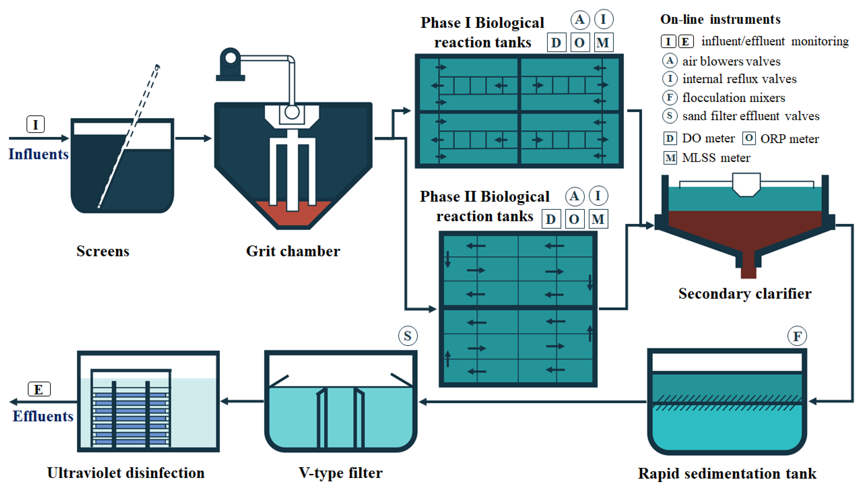
2.1. Study Site Description

The study site was a WWTP in Suzhou City, Jiangsu Province, China. The selected WWTP serves a population of 1,200,000 and treats up to 180,000 m3/day of municipal wastewater. The plant was constructed in two phases with design treatment capacities of 100,000 m3/day and 80,000 m3/day, respectively.
As shown in Figure 1, the wastewater treatment process consisted of pre-treatment (screens), a grit chamber and an activated sludge system, which included anaerobic, anoxic and aerobic tanks, with a hydraulic retention time of 18.2 h. The biological treatment system was followed by a secondary clarifier and then treated with flocculation, sedimentation, sand filtration and chlorination before discharge as the final effluent.

2.2. On-Line Data Source

Data used to develop machine learning method for predicting effluent water quality were obtained from on-line instruments at the WWTP. Generally, the on-line data can be divided into three categories: WWTP influent flow and water quality data, WWTP effluent water quality data and treatment process monitoring and equipment operational data.
For the WWTP influent, there were eight on-line parameters including stage I inflow, stage II inflow, total outflow and influent water quality data for chemical oxygen demand (COD), ammonia (NH3-N), total nitrogen (TN), total phosphorus (TP), and pH. For the WWTP effluent, there were four on-line water quality parameters including COD, NH3-N, TN and TP. The on-line data collection frequency for both WWTP influent and effluent was 1 h. Statistics of WWTP influent and effluent water quality data for the year 2019 is shown in Table 1.
For the monitoring of the WWTP treatment processes, there were 36 on-line monitoring devices, including 6 dissolved oxygen (DO) meters, 4 oxidation–reduction potential (ORP) meters and 3 mixed liquor suspended solids (MLSS) meters in the biological reaction tanks of phase I; 12 DO meters, 7 ORP meters and 4 MLSS meters in the biological reaction tanks of phase II. There were also 42 on-line operational control devices including 8 internal reflux controlling valves in biological reaction tanks, 5 air blowers, 1 total air blower controlling valve, 14 flocculation mixers and 14 sand filter effluent valves. The operation data of all of the above devices were collected in real time, with a data collection frequency of 1 h.

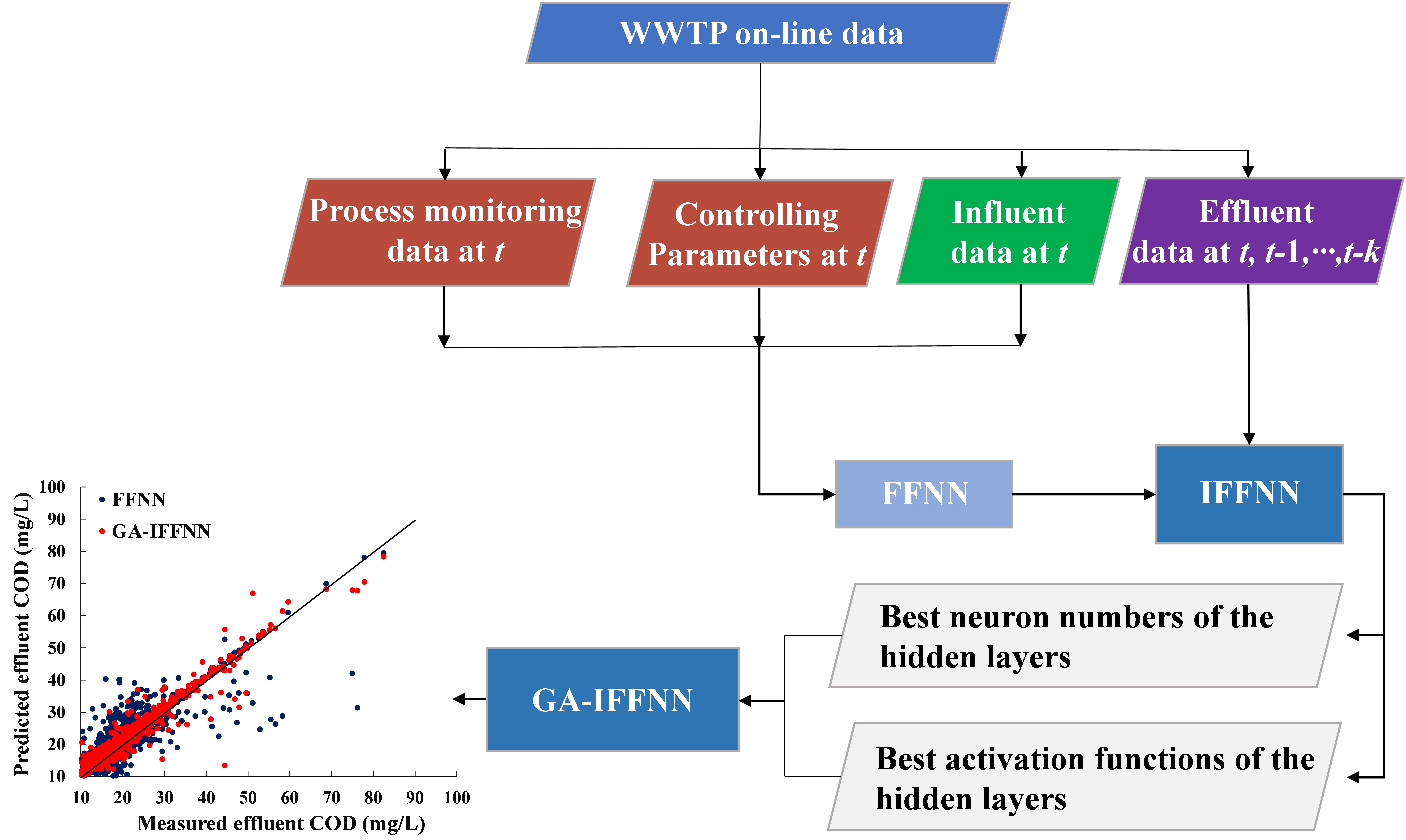
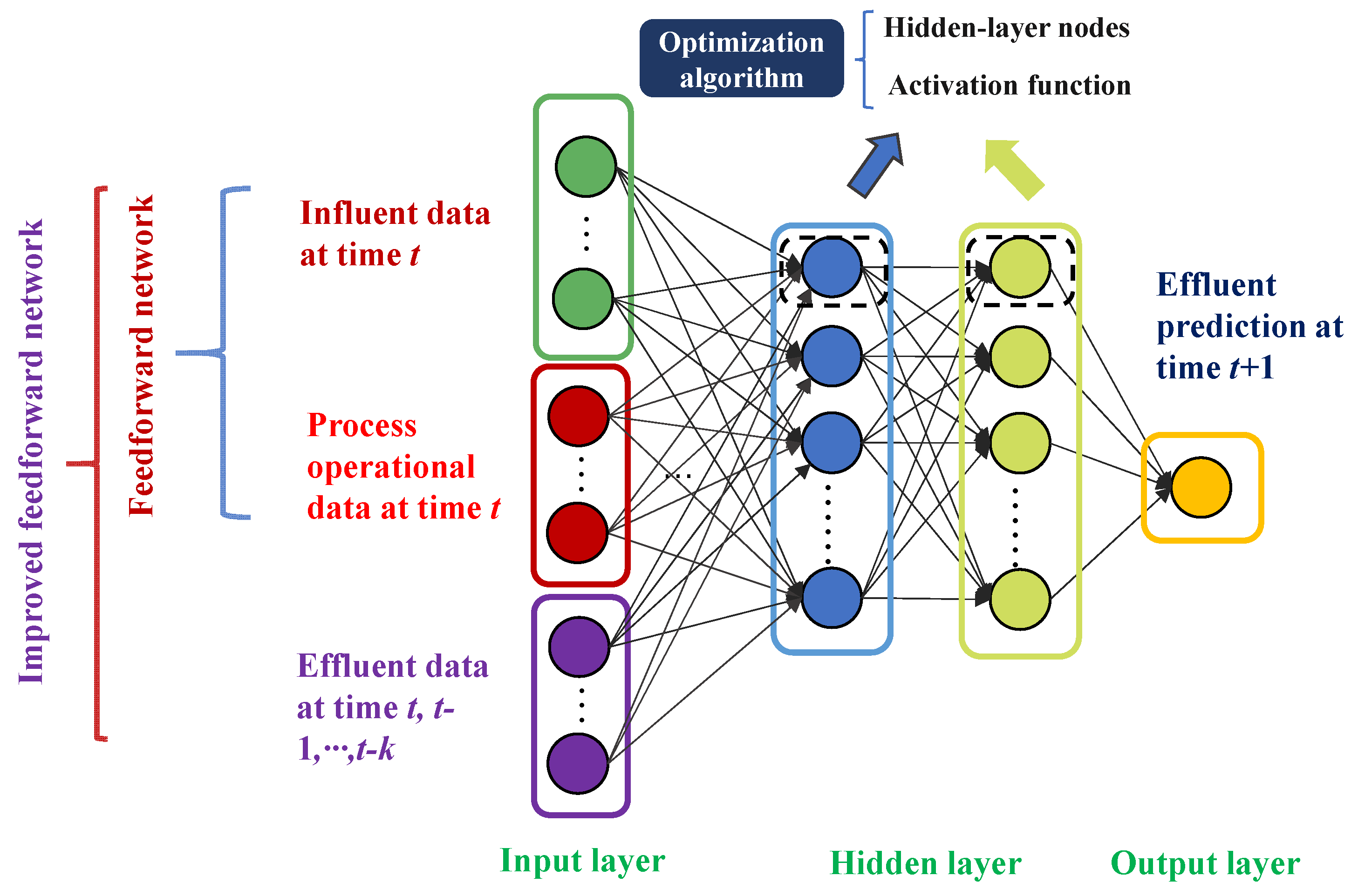
2.3. Motive of Model Structure Design

Commonly, the modeling of pollutant removal through a WWTP is based on the completely mixed reactor model with first-order kinetics:
d c d t = W ( t ) V λ c
where c is the effluent concentration; V is volume of system; W(t) is the real-time influent mass loading, taken as the product:
W ( t ) = Q i n ( t ) C i n ( t )
where Q i n ( t ) is the volumetric flow rate entering the simulated system and C i n ( t ) is influent concentration as a function of time; λ is eigenvalue or characteristic value that represents mass loss related to WWTP outflow and biological treatment processes.
During simulation, the first derivative of c with respect to t can be approximated using a forward difference by
d c i d t Δ c Δ t = c i + 1 c i t i + 1 t i
where c i and c i + 1 are simulated effluent concentration at present and at a future time, t i and t i + 1 , respectively. Substituting Equation (3) into Equation (1) finally yields
C i + 1 = C i + [ W ( t ) V λ C i ] ( t i + 1 t i )
Equation (4) indicates that effluent water quality at a future time is related to both the influent mass loading and effluent water quality at the present time. Based on traditional FFNN design, the influent mass loading ( W ( t ) ) and treatment process parameters (generalized as λ ) are treated as the input layer and effluent water quality is regarded as the output layer. However, the influence of current and historical effluent water quality on future water quality cannot be incorporated into the FFNN. To overcome this problem, we designed an improved feed-forward neural network (IFFNN) that further introduced historical WWTP effluent parameters into ANN input variables, as shown in Figure 2. In this way, the multi-layer perceptron ANN enabled the model to capture the memory of the WWTP operation for future directions in real-time prediction, and it would be efficient to model highly dynamic systems with time series [45]. Depending on the data collection frequency of on-line sensors (1 h data sampling frequency in this case), the model could perform the prediction in a flexible way. Compared to the recurrent neural network model featuring a recurrent hidden state whose activation at each time is dependent on that of the previous time [46,47], the IFFNN developed herein permits the detection of temporal dependences more easily by directly incorporating the previous on-line effluent measurements as inputs.
Generally, the ANN model comprises one or two hidden layers. An increase of hidden layers could reduce predictive accuracy due to overfitting [48]. Therefore, an ANN model with one input layer with multiple input parameters, two hidden layers and one output layer with one neuron (i.e., one designated effluent water quality indicator) was adopted. The number of neurons and most appropriate activation functions in the hidden layer were first specified by the user and then optimized by the optimization algorithm to achieve the best fit between modeling and measured output data.

2.4. Modeling Methodology

2.4.1. IFFNN Module

Let A denote the set of indices i for which a i ( t ) is an external input at moment t , and B denote the set of indices i for which b i ( t k ) , k = 0 , 1 , , n , be the ANN output of the designated parameter at moment t, t − 1, …, t − n, respectively, in the network. We, thus, have
μ i ( t ) = {       a i ( t ) , i f       i A b i ( t k ) , k = 0 ,   1 ,   ,   n , i f       i B
where μ i ( t ) denotes the i-th input element.
The activity of neuron j at moment t is computed by
n e t j ( t ) = i A w j i a i ( t ) + i B w j i b i ( t k )
where w j i is the weight of the link between i-th input element to neuron j.
The output of neuron j is given by passing n e t j ( t ) through the activation function f(.), yielding
y j ( t ) = f ( n e t j ( t ) θ )  
where θ is the threshold to control the output of current neuron.
In Equation (9), a variety of candidate activation functions were used to complete the non-linear transfer from input parameters to output data. Specifically, seven activation functions including Relu, Softmax, Softplus, Softsign, Relu6, Tanh and Sigmoid function were employed in our study.
The performance of the established IFFNN was assessed using the mean absolute percentage error (MAPE) and the coefficient of determination (R2), as described below [49,50]:
MAPE = 1 m i = 1 m | y i y ^ i y i | × 100 %
R 2 = 1 i = 1 n ( y ^ i y i ) 2 i = 1 n ( y ¯ y i ) 2
where y ¯ is the average of y over the n data, y ^ i is the predicted time series of the WWTP effluent water quality data by IFFNN model and y i is the measured time series of the WWTP effluent data.

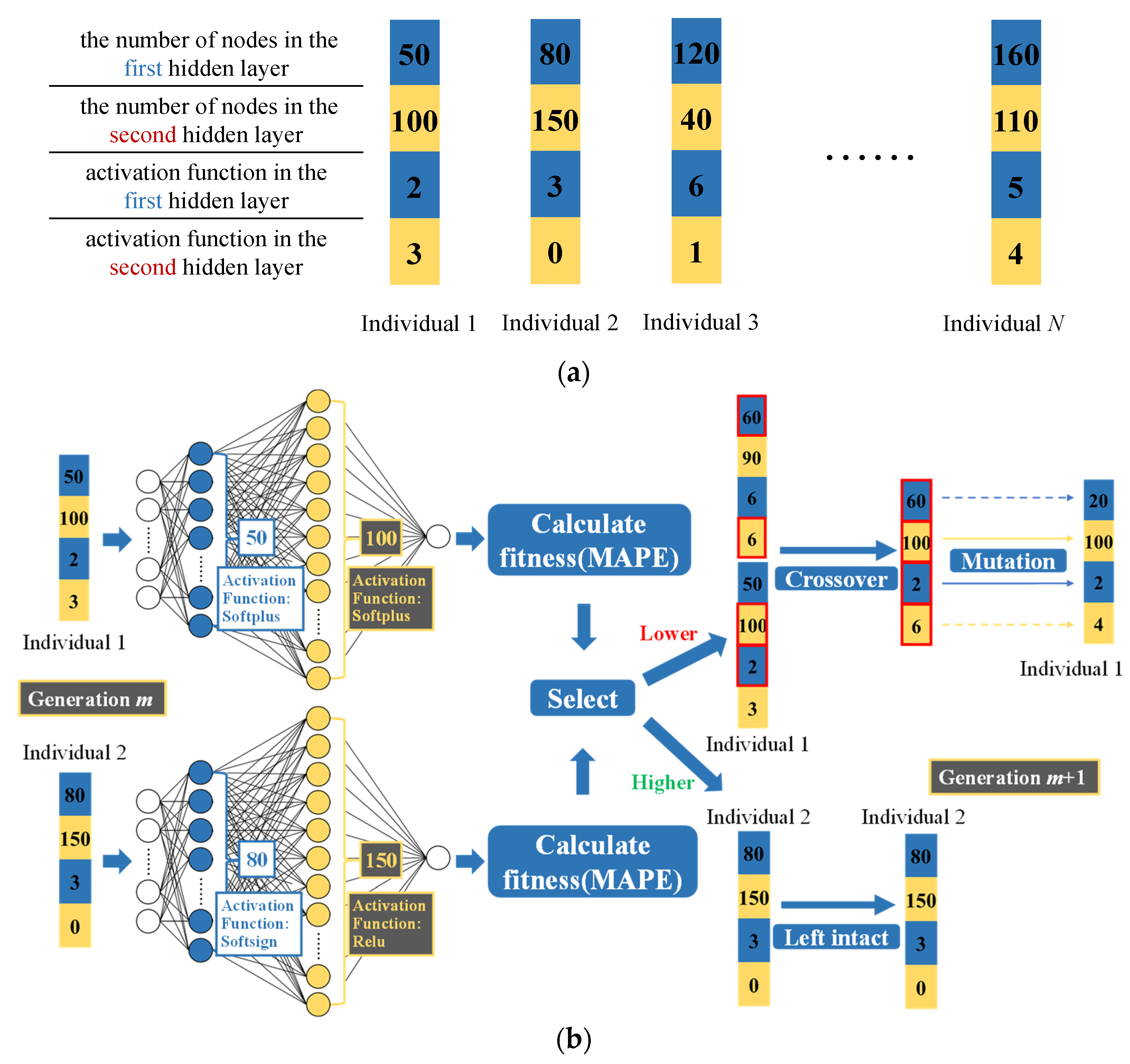
2.4.2. IFFNN Structure Optimization

The search for the best IFFNN structure was based on GA. As an adaptive optimization algorithm based on “survival of the fittest”, GA starts to optimize the problem with an initial population consisting of N chromosomes or individuals. Through the evolution of chromosome groups from generation to generation, including reproduction, crossover and mutation, the algorithm converges to the individual with the best performance for model prediction. Specifically, the optimization steps of GA are performed as follows:
Step 1: Generation of the initial population. Figure 3a gives an initial population with N designated individuals or chromosomes, and each individual is a combination of four optimization parameters, including the number of nodes in the first hidden layer, the number of nodes in the second hidden layer and the activation function in each of the two hidden layers, respectively. For the activation function in the first and second layer of each individual, the numbers 0~6 represent the Relu, Softmax, Softplus, Softsign, Relu6, Tanh and Sigmoid functions, respectively.
Step 2: Population evolution. The tournament method runs a tournament among two individuals chosen at random from the population and selects the winner in accordance with their fitness values (based on MAPE). The winner with better fitness is left intact within the genotype array, enabling the presumptive good genes to be transferred to the next generation (see Figure 3b). The loser with poorer fitness will be modified by crossover and mutation subsequently. In this case, the fitness was based on the MAPE as shown in Equation (8).
Step 3: Crossover and mutation. Crossover is applied on two parent individuals and originates a new individual that contains the combined traits of the parents (see Figure 3b). In the mutation stage, new individuals are produced by changing all or some genes of the selected individuals within the population. Mutation is applied in the offspring generated by the crossover with a mutation probability to which low values are usually assigned.
Steps 2 and 3 were repeated until one individual’s fitness was equal to 1 or until a predefined maximum number of generations was attained.

3. Results and Discussion

3.1. Datasets for ANN Modeling

On-line data in 2019 were used to perform ML prediction for WWTP effluent water quality. Specifically, 1700 groups of data were extracted, where cases of non-steady large variations were included. In this way, the modeling robustness to predict effluent water quality in response to WWTP influent with significant variations could be probed.
These datasets were divided into two subsets of data, namely training and testing data. Previous study showed that 60% training datasets might not be representative enough of the whole dataset [51,52]; however, the performance of the ANN model increased obviously by feeding more training data, with stronger capability and robustness in prediction and extrapolation using 70~89% of the group for training [48]. Apart from a simple percentage cut, there is also the method of k-fold cross validation [53]. Taking 10-fold cross validation as an example, the dataset is divided into 10 parts and 10% of data is rotated for testing in turn, which runs the program 10 times. The modeling performance is then evaluated based on the averaged outcomes of 10 simulations measured by indicators such as MAPE and R2. The k-fold cross validation method is especially efficient for smaller samples, e.g., daily averaged WWTP influent and effluent data. However, considering that hourly WWTP influent and effluent data were available in our case, 80% of the datasets were directly used for training, and the remaining 20% of data points were employed for testing purposes. Specifically, 20% data points (i.e., 340 data points) were chosen pseudorandomly based on the linear congruential method [54].

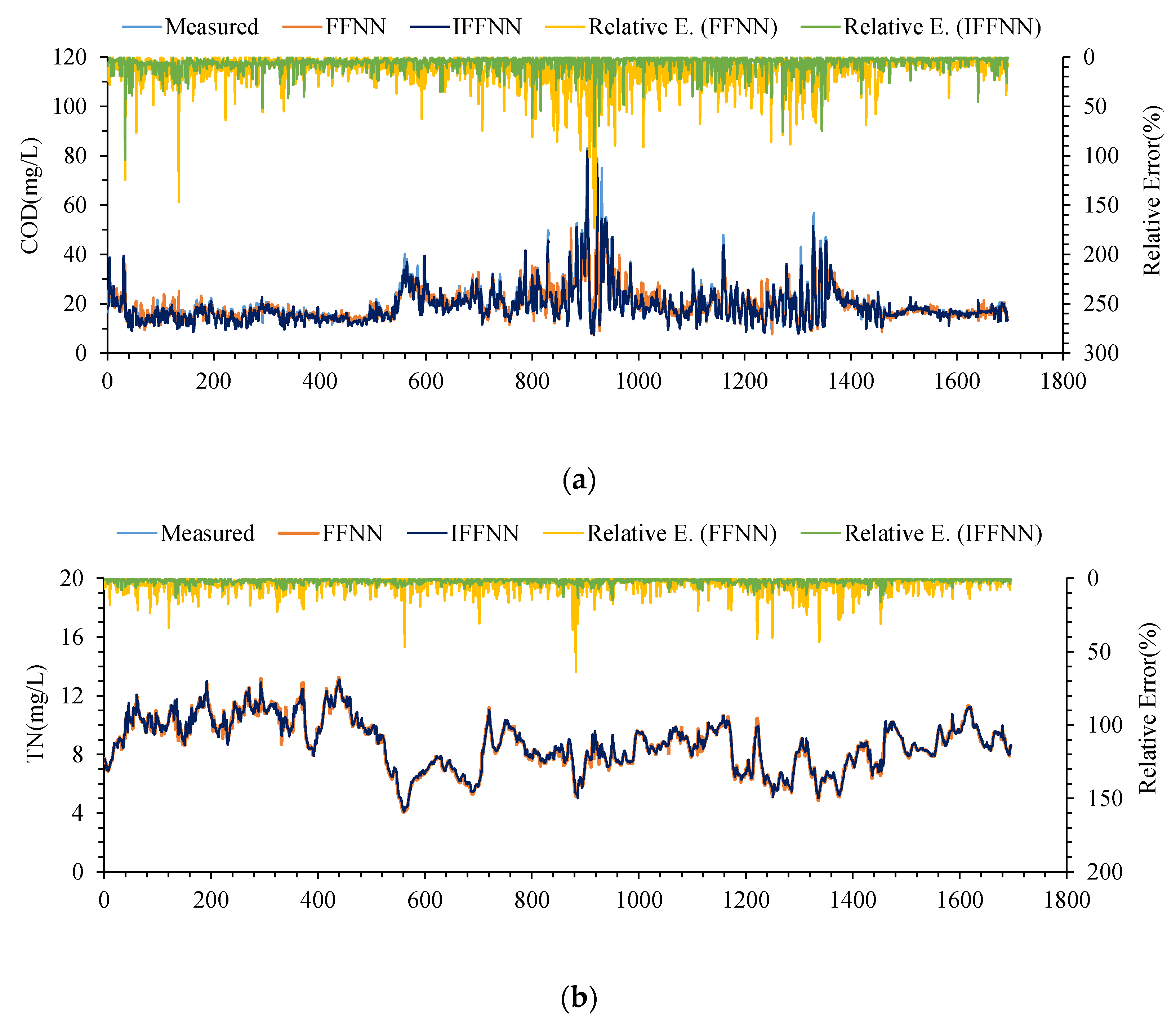
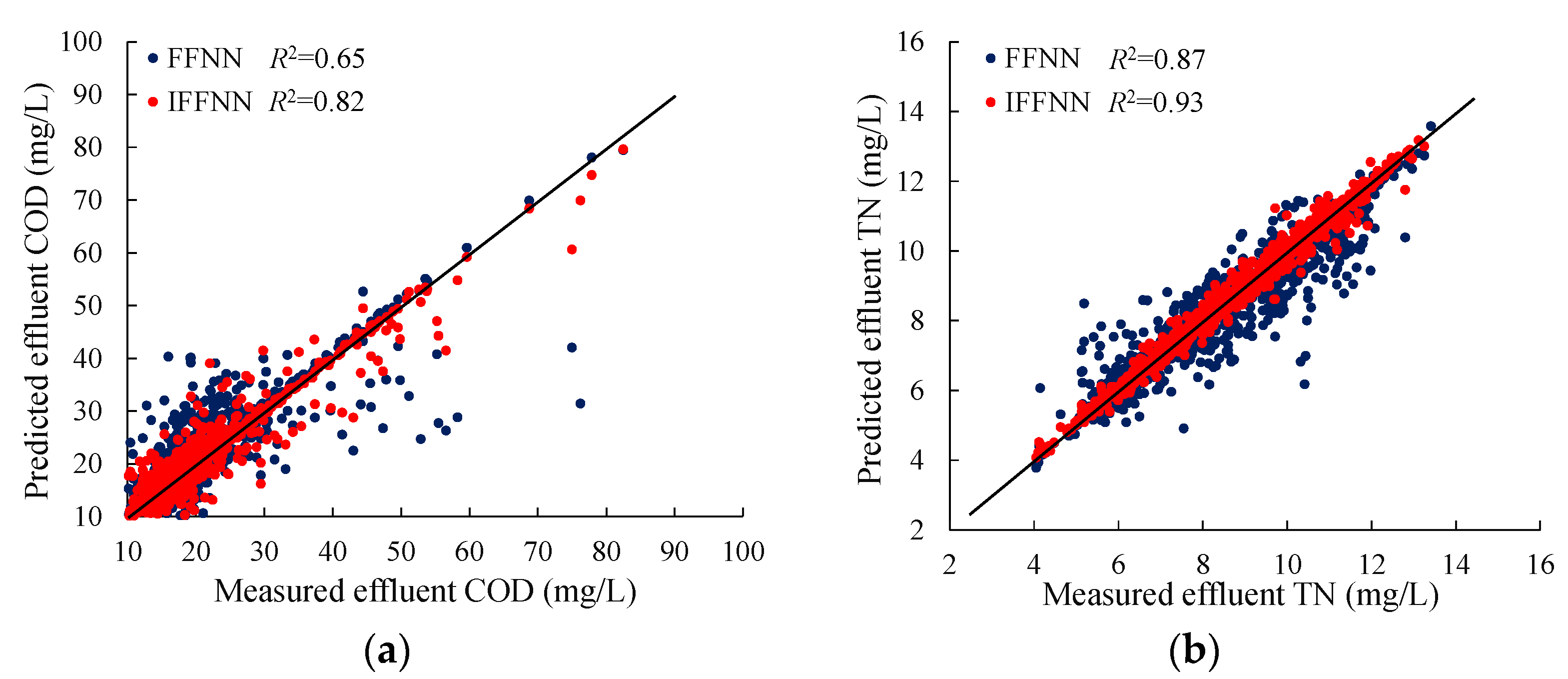
3.2. Modeling Prediction Performance between FFNN and IFFNN

Two separate ANN models for effluent COD and TN were established and trained, considering the two effluent parameters exhibited large real-time variations and effluent COD even had the potential of over-limit discharge. These two models were developed using FFNN and IFFNN structure separately. For both the models, the activation function initially employed for the two hidden layers was Relu6 function.
The neural network was initially designed based on “n-n-n-1” structure, indicating n input variables, n neurons in the first and second hidden layer, and one output variable for designated effluent parameter. For the IFFNN model, 90 parameters including three inflow rates (i.e., total inflow, inflow of phase I and phase II WWTP), 78 on-line treatment process monitoring and equipment operational parameters, 5 influent water quality parameters (COD, NH3-N, TN, TP and pH) at current time step t and 4 effluent water quality parameters (COD, NH3-N, TN, TP) at time step t were employed as input variables. For the traditional FFNN model, 4 effluent water quality parameters at time step t were not included in the input variables, and 86 input variables were employed. Thus, the adopted neural network structure for FFNN and IFFNN was “86-86-86-1” and “90-90-90-1”, respectively.
Comparison of real-time modeling performance based on FFNN and IFFNN is demonstrated and summarized in Figure 4 and Figure 5 and Table 2. Generally, the lower relative error and higher R2 throughout the data groups, and for the two modeled parameters of COD and TN, are indications of the IFFNN’s robustness. Strictly, if taking test datasets as the measurement, the MAPE of the FFNN approximating wastewater treatment processes was 22.0% and 8.4% for effluent COD and TN, respectively, while the MAPE of the predicted COD and TN using the IFFNN was 16.,8% and 4.8% respectively. The performance efficiency of IFFNN modeling improved by 23.6% and 42.9% for COD and TN, respectively, as compared to that of the basic FFNN. If the test datasets were compared based on R2, it increased from 0.20 to 0.47 for effluent COD after the employment of IFFNN. For effluent TN, R2 improved from 0.70 to 0.89 after the use of IFFNN.
The IFFNN models also demonstrated their robustness in predicting the scenarios of effluent under large variations such as shock loading from illicit industrial sewage discharge into sewers in a short period, which would be helpful for enhancing the preparedness of the WWTP operation or adjusting the urban sewer network in advance for leveling off influent pollutant loading. The IFFNN seems to predict the high values better than the FFNN. For example, if setting the effluent COD concentration of 40 mg/L as the risk value of potentially abnormal cases, the performance of the IFFNN model for predicting effluent COD under abnormal cases improved by 43.3% compared to that of the basic FFNN when measured using MAPE. Under this scenario, R2 increased from 0.65 to 0.85 due to the introduction of the IFFNN. As demonstrated in Figure 5a, for the effluent over-limit discharges, the COD concentration predicted by the IFFNN was more likely to approximate the truth; by comparison, the predicted output by the FFNN tended to be under-estimated, which is associated with the lack of a historical memory of the WWTP effluent especially under abnormal influent conditions. Therefore, potential future over-limit discharge could be neglected by the FFNN. By contrast, the IFFNN could present a reasonable prediction. In this way, the IFFNN is superior to the FFNN for determining the WWTP’s proactive actions to tackle potentially abnormal cases.

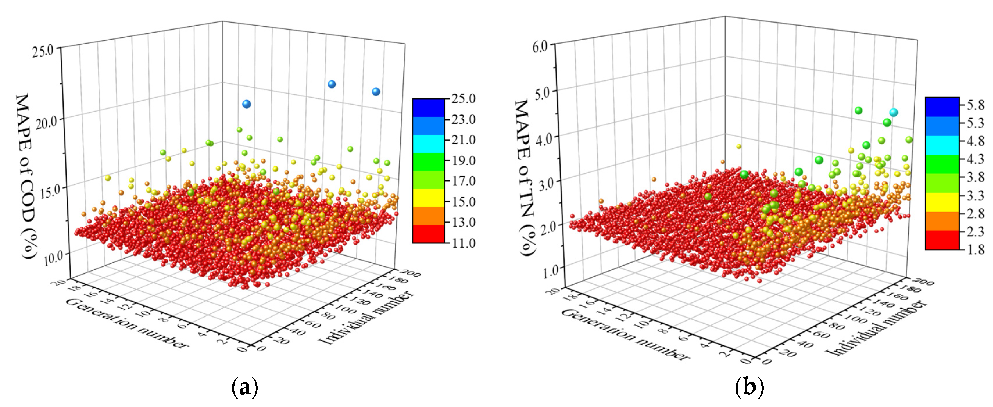
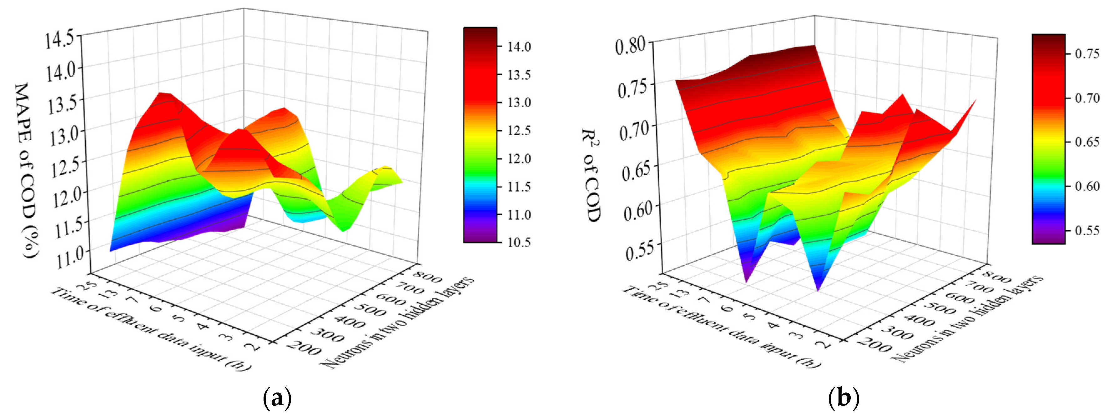
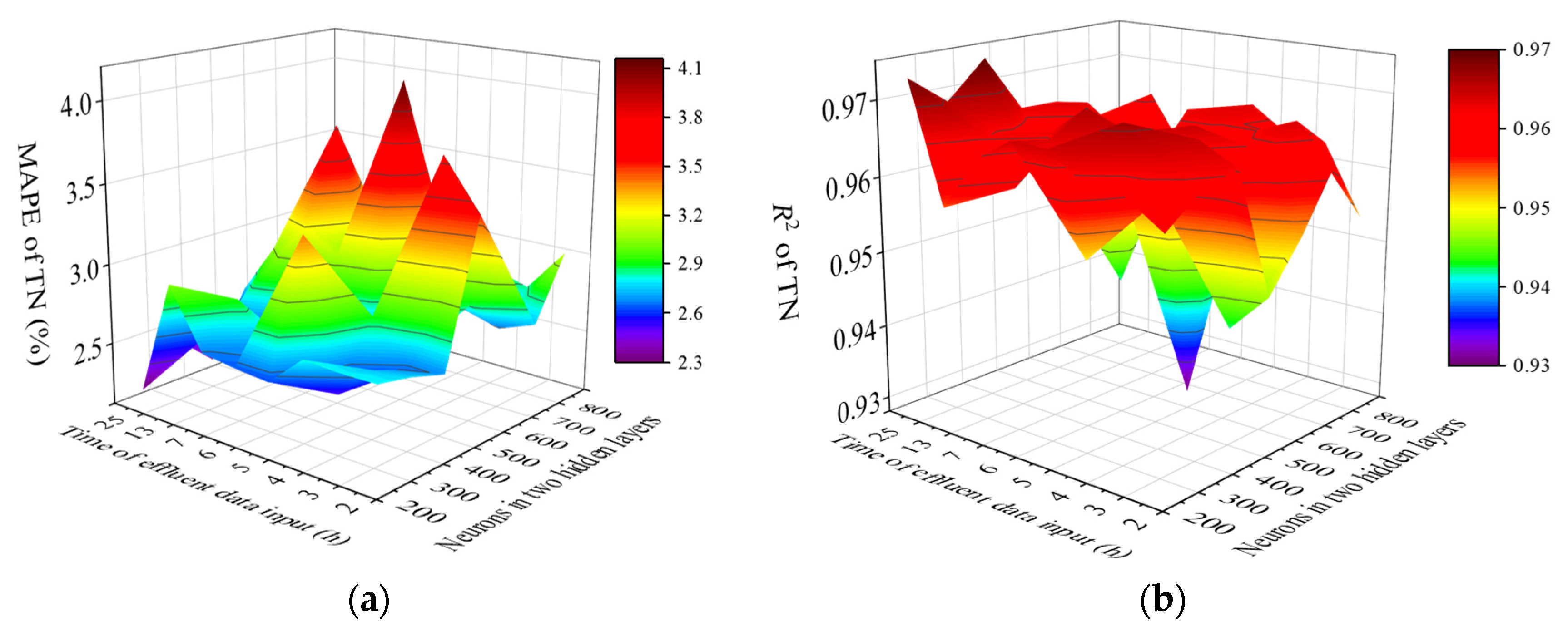
3.3. Modeling Prediction Performance Based on GA-IFFNN

The developed IFFNN model was then optimized with GA (i.e., GA-IFFNN), with the objective of further improving the predicting efficiency for the WWTP effluent water quality. In this case, the minimum and maximum number of artificial neurons in the two hidden layers of the IFFNN were set to 20 and 200, respectively. A random pick was made between the minimum and maximum neurons with a designated interval of 10. The seven above-mentioned candidate activation functions were used. The population size, the number of generations and the probability of mutation of GA were set to 200, 20 and 0.001, respectively. In this way, the GA solved the optimization problem by starting from a random solution and looking for the optimal solution (i.e., optimized FFNN structure) through iteration.
During the self-optimizing process, 20 generations and a corresponding 4000 runs were performed to reach an acceptable goodness of fit between predicted time series data and the measured data at the WWTP outlet. For each generation, through training datasets, the optimized IFFNN structures were determined, and then the modeling prediction performance of GA-IFFNN was further verified using separate test datasets. Figure 6 presents the modeling performance under different generations and associated populations using MAPE as the performance indicator. It shows that the MAPE drops rapidly when the number of generations increases. Generally, for both the predicted effluent indicators, when the size of generations was up to 15, the MAPE fell into a small range, and a further increase of generations could not reduce the MAPE, suggesting that the model optimization was achieved.
The optimized IFFNN structures including the optimized neurons in the first and second hidden layer and the associated activation functions are presented in Table 2. Different water quality parameters correspond to different optimized IFFNN structures, which may be related to different treatment processes for pollutant removal. For example, removal of TN involves anaerobic–anoxic–aerobic reaction tanks, while the treatment of COD is further enhanced by following flocculation–sedimentation processes.
Table 2 demonstrates that, compared with the IFFNN, the outcome of the GA-IFFNN model was better and the prediction error was less. Measured by MAPE, the performance efficiency of GA-IFFNN modeling further improved by 22.6% and 45.8% over that of IFFNN, for the effluent COD and TN, respectively. R2 between the predicted and observed values of effluent COD and TN further improved from 0.47 to 0.63 and from 0.89 to 0.97, respectively, using GA-IFFNN as compared to IFFNN. As a result, the possibility of over-fitting further decreased for effluent COD prediction. In particular, the predicted and measured TN concentration in WWTP effluent discharge were almost identical, showing that the GA-IFFNN model developed here would be a robust ML tool in predicting the real-time WWTP effluent water quality of conventional pollutants.
Furthermore, the modeling prediction efficiency with the increase of artificial neurons in the hidden layers and backward hours for effluent data input was probed, so as to further test the robustness of the optimized IFFNN model. The activation function in the first and second layer remained the same as that of GA-IFFNN in Table 2. The artificial neurons in the hidden layers ranged from 200 to 800, and the backward hours for effluent data input ranged from 1 to 25 h (i.e., at moments t, t − 1, …, t − 24 in Equation (5)). The MAPE and R2 of the test datasets for predicted COD and TN under different neural network complexity are presented in Figure 7 and Figure 8, respectively. These two figures exhibit a fluctuating trend of modeling performance, which is associated with the high non-linearity of the ANN structure.
For all the combination scenarios in Figure 7, the lowest MAPE and highest R2 of test datasets in Figure 7 were 10.5% and 0.76, respectively, with an improvement of 2.5% and 0.13, respectively, compared to the measurements of the originally optimized IFFNN. The best modeling structure for effluent COD prediction is presented in Table 2, which corresponds to 800 artificial neurons in the two hidden layers and backward 25 h for effluent data input. For all the combination scenarios in Figure 8, the best IFFNN structure for effluent TN is also demonstrated in Table 2, with the effluent data input of 25 h and 200 neurons in the two hidden layers. However, very slight improvement was found considering that the originally optimized IFFNN structure coincided well with the truth. Generally, for the real-time prediction of WWTP effluent water quality with potentially large variations, such as effluent COD prediction herein, an MAPE on the order of 10%, could be the best modeling performance to approximate the real outputs. Under this case, relative to the traditional FFNN model, the GA-IFFNN enhanced the prediction performance of effluent COD by 52.3% when measured based on MAPE. The problem of over-fitting could also be overcome significantly through the use of the GA-IFFNN, with the R2 increasing from 0.20 to 0.76 for test datasets of effluent COD. Additionally, the computation time for effluent COD prediction using the originally optimized IFFNN and best IFFNN was 43 and 118 s, respectively (Intel i5-8250U CPU, 1.80 GHz), which did not indicate an obviously increased computation burden in the latter case.

4. Conclusions

To provide highly effective real-time prediction of WWTP effluent water quality, an ML model based on IFFNN coupled with GA was developed. Compared to the traditional FFNN that processes the input assuming the absence of dependency on historical output, the IFFNN incorporated not only current inputs but also recent past outputs from on-line measurements to produce new outputs. Although GA-IFFNN did not depend on the use of internal recurrent hidden state (e.g., the case of recurrent neural network), it was able to model the high non-linearity of the actual WWTPs and capture the dynamics of the WWTP in response to large varied influent properties.
An application in one WWTP with the treatment capacity of 180,000 m3/day in Jiangsu Province, China, demonstrated the effectiveness of the model developed in this study. Measured by MAPE, GA-IFFNN model improved the prediction performance by 52.3% and 72.6% for the test datasets of COD and TN, respectively, relative to the traditional FFNN model. In particular, the problem of over-fitting could be overcome significantly after the use of IFFNN (R2 increased from 0.20 to 0.76 for effluent COD prediction), and the GA-IFFNN modeling output for TN was even almost identical with the monitored data. Comparing to the optimized IFFNN model, further increased model complexity by augmenting artificial neurons in the hidden layers and historical WWTP effluent data input did not necessarily improve prediction performance.
Furthermore, under the scenario of sudden WWTP overloading, the application of the presented ML technologies could be strengthened by regulating the inflow volume rate and concentration in a timely manner (e.g., regulation of urban sewer network through distributed operations of mid-way sewage pumping stations to level off influent shock loading), so as to provide operators with the opportunity to ensure wastewater discharge standards. In this way, the developed model would help adequately address pollutant removal and respond to ensure safe operation of the WWTP as well.
The limitation of this study is that the current IFFNN model lacks an optimal control module to minimize WWTP operational costs in real time, while satisfying the effluent requirements. Thus, future work involves developing an ML model that further combines the current IFFNN with an optimal control algorithm, which will enable its application to both real-time prediction of effluent water quality and WWTP advanced control. Such a model would help adequately address smart WWTP operation and achieve economic benefits in a coordinated way.

Author Contributions

Y.X.: conceptualization, formal analysis, visualization, and writing—original draft preparation; Y.C.: conceptualization and formal analysis; Q.L.: methodology and writing—original draft preparation; H.Y.: conceptualization, methodology, writing—original draft preparation, review and editing and supervision; J.P.: conceptualization, writing—review and editing; M.S.: formal analysis; Y.W.: formal analysis. All authors have read and agreed to the published version of the manuscript.

Funding

This research was funded by the Shanghai Science and Technology Commission (grant no. 20XD1430600) and National Natural Science Foundation of China (grant no. 51979195).

Institutional Review Board Statement

Not applicable.

Informed Consent Statement

Not applicable.

Data Availability Statement

The data presented in this study are available on request from the authors, though some of the data may be held by third parties and permission would need to be sought to obtain those data.

Conflicts of Interest

The authors declare no conflict of interest. The funders had no role in the design of the study; in the collection, analyses, or interpretation of data; in the writing of the manuscript; or in the decision to publish the results.

Abbreviations

ANNArtificial neural network
ASMActivated sludge modeling
CODChemical oxygen demand
DODissolved oxygen
FFNNFeedforward neural network
GAGenetic algorithm
IFFNNImproved feedforward neural network
MAPEMean absolute percentage error
MLMachine learning
MLSSMixed liquor suspended solids
NH3-NAmmonia
ORPOxidation–reduction potential
R2The coefficient of determination
TNTotal nitrogen
TPTotal phosphorus
WWTPWastewater treatment plant

References

  1. Filipe, J.; Bessa, R.J.; Reis, M.; Alves, R.; Povoa, P. Data-driven predictive energy optimization in a wastewater pumping station. Appl. Energy. 2019, 252, 113423. [Google Scholar] [CrossRef] [Green Version]
  2. Plappally, A.K.; Lienhard, V.J.H. Energy requirements for water production, treatment, end use, reclamation, and disposal. Renew. Sustain. Energy Rev. 2012, 16, 4818–4848. [Google Scholar] [CrossRef]
  3. Reifsnyder, S.; Garrido-Baserba, M.; Cecconi, F.; Wong, L.; Ackman, P.; Melitas, N.; Rosso, D. Relationship between manual air valve positioning, water quality and energy usage in activated sludge processes. Water Res. 2020, 173, 115537–115550. [Google Scholar] [CrossRef]
  4. Singh, P.; Carliell-Marquet, C.; Kansal, A. Energy pattern analysis of a wastewater treatment plant. Appl. Water Sci. 2012, 2, 221–226. [Google Scholar] [CrossRef] [Green Version]
  5. Zhang, Z.; Kusiak, A.; Zeng, Y.; Wei, X. Modeling and optimization of a wastewater pumping system with data-mining methods. Appl. Energy 2016, 164, 303–311. [Google Scholar] [CrossRef]
  6. Calise, F.; Eicker, U.; Schumacher, J.; Vicidomini, M. Wastewater Treatment Plant: Modelling and validation of an activated Sludge Process. Energies 2020, 13, 3925. [Google Scholar] [CrossRef]
  7. Jaramillo, F.; Orchard, M.; Munoz, C.; Zamorano, M.; Antileo, C. Advanced strategies to improve nitrification process in sequencing batch reactors—A review. J. Environ. Manag. 2016, 218, 154–164. [Google Scholar] [CrossRef]
  8. Bach, P.M.; Rauch, W.; Mikkelsen, P.S.; McCarthy, D.T.; Deletic, A. A critical review of integrated urban water modelling-urban drainage and beyond. Environ. Modell. Softw. 2014, 54, 88–107. [Google Scholar] [CrossRef]
  9. Rauch, W. Groundbreaking papers in Water Research 1967–2006. Water Res. 2006, 40, 3149. [Google Scholar] [CrossRef]
  10. Henze, M.; Grady, C.P.L., Jr.; Gujer, W.; Marais, G.V.R.; Matsuo, T. A general model for single-sludge wastewater treatment systems. Water Res. 1987, 21, 505–515. [Google Scholar] [CrossRef] [Green Version]
  11. Chen, L.; Tian, Y.; Cao, C.; Zhang, S.; Zhang, S. Sensitivity and uncertainty analyses of an extended ASM3-SMP model describing membrane bioreactor operation. J. Membr. Sci. 2012, 389, 99–109. [Google Scholar] [CrossRef]
  12. Gujer, W.; Henze, M.; Mino, T.; Loosdrecht, M. Activated sludge model no. 3. Water Sci. Technol. 1999, 39, 183–193. [Google Scholar] [CrossRef]
  13. Henze, M.; Gujer, W.; Mino, T.; Matsuo, T.; Wentzel, M.; Marais, G. Wastewater and biomass characterization for the activated sludge model no. 2 biological phosphorus removal. Water Sci. Technol. 1995, 31, 13–23. [Google Scholar] [CrossRef]
  14. Busch, J.; Elixmann, D.; Kühl, P.; Gerkens, C.; Schlöder, J.P.; Bock, H.G.; Marquardt, W. State estimation for large-scale wastewater treatment plants. Water Res. 2013, 47, 4774–4787. [Google Scholar] [CrossRef]
  15. Diehl, S.; Faras, S. Control of an ideal activated sludge process in wastewater treatment via an ODE–PDE model. J. Process Control 2013, 23, 359–381. [Google Scholar] [CrossRef] [Green Version]
  16. Long, S.; Zhao, L.; Liu, H.; Li, J.; Zhou, X.; Liu, Y.; Qiao, Z. A Monte Carlo-based integrated model to optimize the cost and pollution reduction in wastewater treatment processes in a typical comprehensive industrial park in China. Sci. Total Environ. 2019, 647, 1–10. [Google Scholar] [CrossRef]
  17. Moral, H.; Aksoy, A.; Gokcay, C.F. Modeling of the activated sludge process by using artificial neural networks with automated architecture screening. Comput. Chem. Eng. 2008, 32, 2471–2478. [Google Scholar] [CrossRef]
  18. Huang, R.; Ma, C.; Ma, J.; Huangfu, X.; He, Q. Machine learning in natural and engineered water systems. Water Res. 2021, 205, 117666–117689. [Google Scholar] [CrossRef]
  19. Zhao, L.; Dai, T.; Qiao, Z.; Sun, P.; Hao, J.; Yang, K. Application of artificial intelligence to wastewater treatment: A bibliometric analysis and systematic review of technology, economy, management, and wastewater reuse. Process Saf. Environ. Protect. 2020, 133, 169–182. [Google Scholar] [CrossRef]
  20. Zhao, X.; Xu, T.; Ye, Z.; Liu, W. A TensorFlow-based new high-performance computational framework for CFD. J. Hydrodyn. 2020, 32, 735–746. [Google Scholar] [CrossRef]
  21. Kadkhodazadeh, M.; Valikhan Anaraki, M.; Morshed-Bozorgdel, A.; Farzin, S. A new methodology for reference evapotranspiration prediction and uncertainty analysis under climate change conditions based on machine learning, multi criteria decision making and Monte Carlo methods. Sustainability 2022, 14, 2601. [Google Scholar] [CrossRef]
  22. Rashid Niaghi, A.; Hassanijalilian, O.; Shiri, J. Estimation of reference evapotranspiration using spatial and temporal machine learning approaches. Hydrology 2021, 8, 25. [Google Scholar] [CrossRef]
  23. Kadkhodazadeh, M.; Farzin, S. A novel LSSVM model integrated with GBO algorithm to assessment of water quality parameters. Water Resour. Manag. 2021, 35, 3939–3968. [Google Scholar] [CrossRef]
  24. Antwi, P.; Zhang, D.C.; Xiao, L.W.; Kabutey, F.T.; Quashie, F.K.; Luo, W.H.; Meng, J.; Li, J.Z. Modeling the performance of Single-stage Nitrogen removal using anammox and partial nitritation (SNAP) process with backpropagation neural network and response surface methodology. Sci. Total Environ. 2019, 690, 108–120. [Google Scholar] [CrossRef]
  25. Hamed, M.M.; Khalafallah, M.G.; Hassanien, E.A. Prediction of wastewater treatment plant performance using artificial neural networks. Environ. Modell. Softw. 2004, 19, 919–928. [Google Scholar] [CrossRef]
  26. Man, Y.; Hu, Y.; Ren, J. Forecasting COD load in municipal sewage based on ARMA and VAR algorithms. Resour. Conserv. Recycl. 2019, 144, 56–64. [Google Scholar] [CrossRef]
  27. Mandal, S.; Mahapatra, S.S.; Sahu, M.K.; Patel, R.K. Artificial neural network modelling of As (III) removal from water by novel hybrid material. Process Saf. Environ. Prot. 2015, 93, 249–264. [Google Scholar] [CrossRef]
  28. Reynel-Avila, H.E.; Bonilla-Petriciolet, A.; de la Rosa, G. Analysis and modeling of multicomponent sorption of heavy metals on chicken feathers using Taguchi’s experimental designs and artificial neural networks. Desalin. Water Treat. 2015, 55, 1885–1899. [Google Scholar] [CrossRef]
  29. Zhang, W.; Tooker, N.B.; Mueller, A.V. Enabling wastewater treatment process automation: Leveraging innovations in real-time sensing, data analysis, and online controls. Environ. Sci.: Wat. Res. Technol. 2020, 6, 2973–2992. [Google Scholar] [CrossRef]
  30. Giwa, A.; Daer, S.; Ahmed, I.; Marpu, P.R.; Hasan, S.W. Experimental investigation and artificial neural networks ANNs modeling of electrically-enhanced membrane bioreactor for wastewater treatment. J. Water Process Eng. 2016, 11, 88–97. [Google Scholar] [CrossRef]
  31. Khatri, N.; Khatri, K.K.; Sharma, A. Prediction of effluent quality in ICEAS sequential batch reactor using feedforward artificial neural network. Water Sci. Technol. 2019, 80, 213–222. [Google Scholar] [CrossRef]
  32. Yang, S.-S.; Yu, X.-L.; Ding, M.-Q.; He, L.; Cao, G.-L.; Zhao, L.; Tao, Y.; Pang, J.-W.; Bai, S.-W.; Ding, J.; et al. Simulating a combined lysis-cryptic and biological nitrogen removal system treating domestic wastewater at low C/N ratios using artificial neural network. Water Res. 2021, 189, 116576. [Google Scholar] [CrossRef]
  33. Nourani, V.; Asghari, P.; Sharghi, E. Artificial intelligence based ensemble modeling of wastewater treatment plant using jittered data. J. Clean. Prod. 2021, 291, 125772. [Google Scholar] [CrossRef]
  34. Sharghi, E.; Nourani, V.; AliAshrafi, A.; Gokcekus, H. Monitoring effluent quality of wastewater treatment plant by clustering based artificial neural network method. Desalination Water Treat. 2019, 164, 86–97. [Google Scholar] [CrossRef]
  35. Mahmod, N.; Wahab, N.A. Dynamic modelling of aerobic granular sludge artificial neural networks. Int. Jo. Electr. Comput. Eng. 2017, 7, 1568–1573. [Google Scholar] [CrossRef]
  36. Yu, P.; Cao, J.; Jegatheesan, V.; Du, X. A real-time BOD estimation method in wastewater treatment process based on an optimized extreme learning machine. Appl. Sci. 2019, 9, 523. [Google Scholar] [CrossRef] [Green Version]
  37. Al Aani, S.; Bonny, T.; Hasan, S.W.; Hilal, N. Can machine language and artificial intelligence revolutionize process automation for water treatment and desalination? Desalination 2019, 458, 84–96. [Google Scholar] [CrossRef]
  38. Zhao, Z.; Yin, H.; Xu, Z.; Peng, J.; Yu, Z. Pin-pointing groundwater infiltration into urban sewers using chemical tracer in conjunction with physically based optimization model. Water Res. 2020, 175, 115689–115698. [Google Scholar] [CrossRef]
  39. Badrnezhad, R.; Mirza, B. Modeling and optimization of cross-flow ultrafiltration using hybrid neural network-genetic algorithm approach. J. Ind. Eng. Chem. 2014, 20, 528–543. [Google Scholar] [CrossRef]
  40. Ren, F.; Hu, H.; Tang, H. Active flow control using machine learning: A brief review. J. Hydrodyn. 2020, 32, 247–253. [Google Scholar] [CrossRef]
  41. Schubert, M.; Muffler, A.; Mourad, S. The use of a radial basis neural network and genetic algorithm for improving the efficiency of laccase-mediated dye decolourization. J. Biotechnol. 2012, 161, 429–436. [Google Scholar] [CrossRef]
  42. Fernandez de Canete, J.; del Saz-Orozco, P.; Gómez-de-Gabriel, J.; Baratti, J.; Ruano, A.; Rivas-Blanco, I. Control and soft sensing strategies for a wastewater treatment plant. Comput. Chem. Eng. 2021, 144, 107146. [Google Scholar] [CrossRef]
  43. Huang, M.; Wei, H.; Wan, J.; Ma, Y.; Chen, X. Multi-objective optimisation for design and operation of anaerobic digestion using GA-ANN and NSGA-II. J. Chem. Technol. Biotechnol. 2016, 91, 226–233. [Google Scholar] [CrossRef]
  44. Lotfi, K.; Bonakdari, H.; Ebtehaj, I.; Mjalli, F.S.; Zeynoddin, M.; Delatolla, R.; Gharabaghi, B. Predicting wastewater treatment plant quality parameters using a novel hybrid linear-nonlinear methodology. J. Environ. Manag. 2019, 240, 463–474. [Google Scholar] [CrossRef]
  45. Ghaderpour, E.; Pagiatakis, S.D.; Hassan, Q.K. A survey on change detection and time series analysis with applications. Appl. Sci. 2021, 11, 6141. [Google Scholar] [CrossRef]
  46. Dairi, A.; Cheng, T.; Harrou, F.; Sun, Y.; Leiknes, T. Deep learning approach for sustainable WWTP operation: A case study on data-driven influent conditions monitoring. Sustain. Cities Soc. 2019, 50, 101670. [Google Scholar] [CrossRef]
  47. Qiao, J.; Huang, X.; Han, H. Recurrent neural network-based control for wastewater treatment process. In Proceedings of the Advances in Neural Networks—ISNN 2012; Springer: Berlin/Heidelberg, Germany, 2012; pp. 496–506. [Google Scholar]
  48. Zhang, Y.; Gao, X.; Smith, K.; Inial, G.; Liu, S.; Conil, L.B.; Pan, B. Integrating water quality and operation into prediction of water production in drinking water treatment plants by genetic algorithm enhanced artificial neural network. Water Res. 2019, 164, 114888–114899. [Google Scholar] [CrossRef]
  49. Chakraborty, T.; Chakraborty, A.K.; Chattopadhyay, S. A novel distribution-free hybrid regression model for manufacturing process efficiency improvement. J. Comput. Appl. Math. 2019, 362, 130–142. [Google Scholar] [CrossRef] [Green Version]
  50. Asadi, A.; Verma, A.; Yang, K.; Mejabi, B. Wastewater treatment aeration process optimization: A data mining approach. J. Environ. Manag. 2017, 203, 630–639. [Google Scholar] [CrossRef]
  51. Abrahart, R.J.; Dawson, C.W.; See, L.M.; Mount, N.J.; Shamseldin, A.Y. Discussion of “Evapotranspiration modelling using support vector machines”. Hydrol. Sci. J. 2010, 55, 1442–1450. [Google Scholar] [CrossRef]
  52. Maier, H.R.; Jain, A.; Dandy, G.C.; Sudheer, K.P. Methods used for the development of neural networks for the prediction of water resource variables in river systems: Current status and future directions. Environ. Model. Softw. 2010, 25, 891–909. [Google Scholar] [CrossRef]
  53. Xiong, Z.; Cui, Y.; Liu, Z.; Zhao, Y.; Hu, M.; Hu, J. Evaluating explorative prediction power of machine learning algorithms for materials discovery using k-fold forward cross-validation. Comp. Mater. Sci. 2020, 171, 109203. [Google Scholar] [CrossRef]
  54. Steele, G.L., Jr.; Vigna, S. LXM: Better Splittable Pseudorandom Number Generators (and Almost as Fast). Proc. ACM Program. Lang. 2021, 5, 1–31. [Google Scholar] [CrossRef]
Figure 1. Schematic representation of treatment processes and on-line instruments in the selected WWTP.
Water 14 01053 g001
Figure 2. Structure of IFFNN modeling for predicting future WWTP effluent water quality.
Water 14 01053 g002
Figure 3. Schematic diagram of GA for the finding the ANN structure with the best modeling performance: (a) individual structure and (b) GA evolution procedure.
Water 14 01053 g003
Figure 4. Comparison of real-time WWTP effluent prediction between the FFNN and IFFNN models for the water quality parameters (a) COD and (b) TN, respectively.
Water 14 01053 g004
Figure 5. Comparison of modeling performance efficiency between FFNN and IFFNN for the water quality indicators (a) COD and (b) TN, respectively.
Water 14 01053 g005
Figure 6. Modeling prediction performance as a function of GA generation and individual number for effluent water quality for (a) COD and (b) TN, respectively.
Water 14 01053 g006
Figure 7. Change of IFFNN performance for COD with artificial neurons in the two hidden layers and time period of historical effluent data input: (a) MAPE and (b) R2 of test datasets.
Water 14 01053 g007
Figure 8. Change of IFFNN performance for TN with artificial neurons in the two hidden layers and time period of historical effluent data input: (a) MAPE and (b) R2 of test datasets.
Water 14 01053 g008
Table 1. Statistics of WWTP influent and effluent water quality data for the study site.
No.ParametersUnitAve.Standard DeviationMax.Min.Grade 1-A Discharge Standard
1Influent CODmg/L32092.979670.1/
2Influent NH3-Nmg/L22.33.6730.015.1/
3Influent TNmg/L49.07.5759.930.1/
4Influent TPmg/L3.451.088.861.31/
5pH/7.700.499.256.86/
6Effluent CODmg/L19.57.5682.57.8850
7Effluent NH3-Nmg/L0.100.010.150.065 (8) 1
8Effluent TNmg/L8.671.7413.34.0515
9Effluent TPmg/L0.120.030.200.030.5
1 The discharge standard for NH3-N was 8.0 mg/L at a water temperature below 13 °C.
Table 2. Modeling structures and performances for the predicted WWTP effluent water quality.
(a) COD
Modeling TypeTime of Effluent Data Input (h)ANN StructureTraining DatasetTest Dataset
MAPER2MAPER2
FFNN1 a) 86-86-86-16.3%0.8422.0%0.20
b) Relu6-Relu6
IFFNN1a) 90-90-90-14.9%0.9216.8%0.47
b) Relu6- Relu6
GA-IFFNN1a) 90-160-180-13.7%0.9513.0%0.63
b) Relu-Tanh
GA-IFFNN25 a) 186-800-800-13.6%0.9510.5%0.76
b) Relu-Tanh
(b) TN
Modeling TypeTime of Effluent Data Input (h)ANN StructureTraining DatasetTest Dataset
MAPER2MAPER2
FFNN1a) 86-86-86-13.6%0.928.4%0.70
b) Relu6-Relu6
IFFNN1a) 90-90-90-12.8%0.954.8%0.89
b) Relu6-Relu6
GA-IFFNN1a) 90-100-180-10.6%0.992.6%0.97
b) Sigmoid-Relu
GA-IFFNN25a) 186-200-200-10.6%0.992.3%0.97
b) Sigmoid-Relu
Note: a) represents the number of neurons in the input layer, first hidden layer, second hidden layer and output layer, respectively; b) represents the activation function in the first and second layer, respectively.
Publisher’s Note: MDPI stays neutral with regard to jurisdictional claims in published maps and institutional affiliations.

