
Regional Rainfall Regimes Affect the Sensitivity of the Huff Quartile Classification to the Method of Event Delineation


School of Earth, Atmosphere and Environment, Monash University, Wellington Road, Melbourne 3800, Australia
Water 2022, 14(7), 1047; https://doi.org/10.3390/w14071047
Submission received: 2 February 2022
/
Revised: 15 March 2022
/
Accepted: 24 March 2022
/
Published: 26 March 2022
(This article belongs to the Section Ecohydrology)
Abstract
:The widely used Huff quartile approach classifies rainfall events according to which quarter of their duration contains the largest rainfall depth. The rainfall events themselves are often delineated by specifying a minimum rainless interevent time (MIT) that must precede and follow a period of rainfall for it to be identified as a separate event. However, there is no standard or universally applicable value of this MIT criterion. Some studies have stipulated as little as 15 rainless minutes to mark the start of a new event, whilst others have required 24 h or more. The present work investigates how the adoption of different values of the MIT criterion, based, for instance, on the response time of a catchment or the drying time of a vegetation canopy, affects the Huff quartile classification. To date, this has not been explored. To address this issue, the Huff classification is herein applied to data from two Australian ground observing stations, one arid continental and one wet tropical. For each location, rainfall events were delineated using values of the MIT criterion ranging from 30 min to 24 h. In comparison with the 6 h MIT adopted by Huff (1967) as being appropriate for locations in the eastern USA, results show that, for instance, the proportion of events classified as 4Q ranges from 70.9% larger when events are delineated with a MIT = 30 min to 50.8% smaller when events are delineated using a MIT = 24 h. Moreover, the changes in the Huff classification that result from the use of different MIT values were not the same in wet tropical and arid locations. It is argued here that these findings reflect complexity in the arrival of rainfall, including differences in event duration and intraevent intermittency, that cannot be captured in the Huff classification system. Relevant rainfall regime characteristics such as these are likely to vary geographically, and the differences shown between the eastern USA and the two Australian locations are only examples of what is likely a more general effect. The results show that there is no single and generally applicable ‘Huff classification’ process, and that rather than a 6 h MIT being applicable everywhere, different MIT durations are needed in locations having differing rainfall regimes.
1. Introduction
The classification of the intensity profile (IP) of a rainfall event—the time-varying sequence of intensities through the duration of rainfall, frequently including temporary cessations of rain—remains a challenge. Most schemes could be regarded as being of a broad ‘classificatory’ nature, relying on one or a few indices that are capable of embodying only one or a few selected aspects of the IP. For instance, some descriptors rely on quantifying just the highest short-interval intensities, through the use of indices such as I5, I15, I30, and so on. Others include the ratio of the rainfall amount prior to the intensity maximum to that following it [1]. A widely used scheme relies on subdividing a rainfall event into three or four subsections of equal duration. In the former, dating from the work of Horner and Jens (1942) [2], events are classified as ‘advanced’ if the largest share of the rainfall arrives in the first third of the duration, ‘delayed’ if it arrives in the last third, or ‘intermediate’ otherwise. The use of four divisions is more common and is exemplified by the Huff quartile approach (Huff 1967) [3], in which events are categorised according to which quartile has the largest rainfall depth (and hence the highest mean rainfall rate), such that events are referred to as ‘first quartile’ (hereafter 1Q), ‘fourth quartile’ (hereafter 4Q), etc., to reflect this ‘dominant quartile’ [4,5,6,7]. By identifying the quartile with the heaviest rainfall, Huff intended to provide a tool that would help in the analysis of urban drainage problems, soil erosion, and related topics. The Huff quartile classification has seen wide adoption in work seeking to characterise rainfall events in some research location of interest, often to guide the development of representative synthetic ‘design storms’ for use in planning and hydrological modelling work for that region [8]. The Huff quartile categories of local rainfall are also used in some studies to guide the design of experiments exploring runoff production, soil erosion, and other land surface processes, employing, for instance, rainfall simulation methods designed to mimic the quartile type of local natural rainfall [9]. The Huff quartile classification is also widely used as a tool in the climatological description and analysis of regional rainfall regimes or climatologies [10].
Further analysis of the Huff (1967) [3] quartile classification system is the subject of the present paper. Though widely used, it appears to remain incompletely explored. The particular issue examined here is the possible influence on the Huff classification of the means by which the rainfall events are themselves delineated. Huff (1967) [3] separated the rainfall events in his study by stipulating a 6 h rainless period before and following each delineated event. This has subsequently been referred to as the ‘interevent time’ [11], ‘minimum dry period duration’ [12,13], the ‘minimum interevent time’ (MIT) [14,15,16], or the ‘interevent time definition’ (IETD) [17]. ‘MIT’ is adopted here. Whilst this is by far the most common method used to delineate rainfall events, there is no universal agreement on the most appropriate value for the MIT criterion. MIT values from 30 min to 7 days have been used [11,14,18]. Indeed, an appropriate MIT can be selected on the basis of various criteria, depending on the research purpose for which the rainfall events are being classified. For instance, in studies of interception loss on vegetation canopies, the MIT has been related to the canopy drying-time needed between showers, such that at the beginning of a rainfall event, the canopy has had sufficient time after the previous rainfall to become dry [19]. In studies of catchment runoff, the MIT has been related to the response time of the catchment, such that the outlet has returned to baseflow prior to the next event [17]. Other contexts include the link between rainfall and the triggering of landslides, mudflows, and the like, or the way in which rainfall events drive urban flash flooding from relatively impervious surfaces. Achieving the statistical independence of events, regardless of their impact at the land surface, has also been employed as a means of deciding on a value for the MIT. However, this has resulted in different MIT values for different geographical regions and some problems with the hydrological application of the resulting events. Driscoll et al. (1989) [20], for instance, found the ‘statistical independence’ approach inappropriate because it resulted in MIT values for some parts of the USA reaching 300 h (12.5 days), resulting in abnormally large rainfall depths and long durations as well as very low mean rainfall rates in the rainfall events that were thereby delineated.
In summary, the MIT value can be selected solely on the basis of criteria applied to the rainfall record (e.g., a specified rainless period between events) or can be based on other criteria altogether such as the timing of runoff response in a catchment area. These different methods can yield quite different values of MIT for the same geographical location [17]. The most appropriate approach is rarely clear, and arbitrary choices are sometimes made. The focus here, therefore, is the issue of how the choice of an MIT criterion for delineating rainfall events might affect their Huff quartile classification. Several specific questions are asked:
- -
- Does the choice of the MIT (1 h, 6 h, 12 h, etc.) significantly affect the proportions of events classified as 1Q, 2Q, etc., using the Huff quartile classification?
- -
- If the outcome of the Huff classification is affected by the choice of a MIT, does any change in proportions emerge equally in all quartiles, or in only one or more, and how large is any effect on the quartile classification?
- -
- How are the mean properties of a sample of quartiles from a given location (such as the mean rainfall rate of Q1, Q2, and so on) affected by the MIT criterion?
- -
- What might account for any dependencies of the Huff classification on the choice of the MIT criterion? In particular, does the dependence in some way arise as a consequence of the local rainfall regime (monsoonal, frontal, orographic, convective, etc.), or is it wholly a function of the MIT approach?
By examining these issues, the overarching objective is to ask whether the Huff quartile classification results in meaningful descriptions of the IP of rainfall events, or whether it is overly influenced by the value of the MIT and the nature of the local rainfall regime, such that owing to one or both influences, quartile frequencies from one study might not be strictly comparable with those from any other study.
2. Materials and Methods
The analysis presented below uses high-resolution rainfall data from two Australian ground observing stations. The first is located on the Atherton Tableland in the wet tropical climate of far northern Queensland, Australia, near the township of Millaa Millaa (145°39′ E, 17°27′ S). This site, which receives an annual rainfall of about 3000 mm, lies about 700 m above sea level. It has a strongly seasonal climate with a prominent wet season extending from December to June. Prolonged rainfall results from onshore southeast trade winds that rise over the rugged terrain just inland from the coast. This results in orographically enhanced rainfall of moderate intensity. Convective thunderstorms of higher intensity also occur in a stormy ‘buildup’ period prior to the commencement of the wet season. These storms typically occur in November and December. The second observing site is arid and is located on the Fowlers Gap Arid Zone Research Station in far western New South Wales, Australia, about 100 km north of the regional city of Broken Hill (141°42′ E, 31°05′ S). This site receives a mean annual rainfall of about 220 mm, with high interannual variability associated with the El Niño—Southern Oscillation phenomena (Pui et al. 2012 [21]). Afternoon convective storms can be quite intense, though relatively short-lived, and there can be periods of up to several months with no rainfall.
The intention in using two strongly contrasting observing sites is to enquire whether the findings on the several objectives just outlined are the same at both, or differ according to the rainfall regime (rainfall climatology) of the site. If the latter is shown to be the case, then this amounts to an important complication in interpreting Huff classifications. Specifically, it would not be clear if a difference in, for instance, the proportion of Q1 events between different research sites or studies adopting a different MIT criterion resulted from the adoption of different MIT criteria or from an actual difference in the IPs of the rainfall events. This argument will be made clearer with actual examples following the presentation of results below.
Both field sites were equipped with tipping-bucket rain gauges (TBRGs) and event data loggers which recorded the Gregorian date and time of each bucket tip event to the nearest 1 s. The Millaa Millaa (hereafter MM) record, using a TBRG with 0.2 mm sensitivity, includes about 3.5 years of data and 9000 mm of rainfall. The Fowlers Gap (hereafter FG) record, using a TBRG with 0.5 mm sensitivity, includes about 10 years of data and about 2600 mm of rainfall. Both records are complete, with no missing data.
Data processing to identify individual rainfall events worked from the raw, unaggregated record of individual bucket tip events. These were converted from the Gregorian calendar to Modified Julian dates, and separate rainfall events were delineated using the widely adopted minimum interevent time (MIT) approach [22,23,24,25]. An individual tip event marked the beginning and end of each rainfall event. This allowed the duration of an event to be much more precisely recorded than when using hourly or other aggregated data, since in delivering the rainfall recorded in the first hour, the rain may in fact have started in the 55th minute. This would result in an event duration that was erroneously almost 1 h too long. The same applies at the end of an event, such that using hourly data, the event duration could be estimated as almost 2 h longer than the true duration. Moreover, the estimated rainfall depth and intensity in both Q1 and Q4 could then also be erroneous. When using smaller values of the MIT, this poses a serious level of uncertainty in event characteristics. In support of the research objectives outlined previously, multiple values of the MIT criterion were used, viz., 30, 60, 120, 240, 360, 720, and 1440 min. All of these values have been adopted in published studies [11,14] and as noted earlier, the third-largest value, 360 min (6 h), was the value adopted by Huff (1967) [3].
Selection and Processing of Rainfall Events
Only events including at least five bucket tip events were processed. This excluded a significant number of isolated single-tip events for which no duration or intensity could be estimated. Shorter values of the MIT result in the delineation of rainfall events that are on average shorter and of smaller total depth. When applying small values of the MIT, the quartiles are typically also consequently shorter, and preliminary data processing revealed that tied quartiles, that is, two or more quartiles with the same total rainfall, were not uncommon. At MM, there were 294 ties (affecting 22.5% of rainfall events) for a MIT = 30 min. For a MIT = 360 min, only 20 ties were encountered (affecting about 6% of rainfall events). Events with tied quartiles cannot be classified using the Huff quartile system which requires the single wettest quartile to be identified. This issue can be exemplified by MM event 3277, a small event including 27 tip events for a rainfall of 5.4 mm. This event had a duration of 0.91 h, and a mean rainfall rate of 5.92 mm h−1. The quartile depths were 1.8 mm, 0.6 mm, 1.2 mm, and 1.8 mm, such that Q1 and Q4 recorded the same depth.
To avoid the exclusion of multiple rainfall events with tied quartiles, a procedure was adopted to eliminate ties. For each tie, a single random number from a set uniformly distributed in (0,1) was generated. If this number was <0.5, the lower of the tied quartiles was identified as the wettest, and if the number was ≥0.5, the higher of the quartiles was identified as the wettest. Approximately equal numbers of ties were resolved using this approach to either the lower or the higher quartile. Checking all possible quartile ties was undertaken, including, for instance, Q1==Q2, Q2==Q3, Q3==Q4, Q1==Q4, and so on (‘==’ indicates quartiles that recorded the same rainfall depth). Few ties were encountered in rainfall events delineated using larger values of the MIT criterion. For instance, at MM, using a MIT = 1440 min, ties occurred just twice, representing only ~1.6% of events. At FG using a MIT = 1440 min, slightly more ties (8) occurred, in 5.6% of rainfall events. To the writer’s knowledge, this issue connected with Huff quartile classification has not previously been evaluated, but it can be managed without introducing bias by using the procedure just outlined. Ties could also be resolved by adding some arbitrary, very small rainfall at random to one or other of the tied quartiles—perhaps 0.05 mm. But the procedure just outlined achieves the same result with no effect on the rainfall amounts.
Additional data processing was undertaken to determine the mean rainfall intensity of each quartile for every delineated rainfall event and averaged for each quartile across all rainfall events, as well as for the number of quartiles that recorded no rainfall, for all tested values of the MIT. The maximum quartile rainfall intensity and the number of rainless quartiles were determined for each event and for every value of the MIT criterion. These analyses were undertaken to characterise the kinds of outcomes that can result when differing MIT criteria are employed in terms of the Huff quartile classification..
Intensity was estimated from the unaggregated intertip times of the pluviograph bucket mechanisms. This assumes that the rainfall rate was constant between tip events and can be expressed as
where R is the rainfall rate (mm h−1) between times T1 and T2, the clock times of two successive bucket tip events (expressed in hours) and ΔV is the recorded rain depth (mm) that is a function of the bucket capacity.
R(T2 − T1) = ΔV/(T2 − T1)
The mean intensity for entire rainfall events (Iave) was likewise derived from the unaggregated ITT data (expressed in minutes) from the value of N, the number of ITTs in the rainfall event, and ΔV, the bucket capacity of the TBRG.
At MM, 73.0% of ITTs had durations of ≤6 min, and 36.5% ≤ 1 min. At FG, the corresponding fractions were 53.9% ≤ 6 min and 18.5% ≤ 1 min. Thus, the use of unaggregated ITTs is considered to be largely unaffected by intensity variations through one or a few minutes and certainly provides higher resolution intensity data than can be obtained from time-aggregated data, such as 15 min or 1 h rainfall totals.
3. Results
3.1. The Mean Properties of All Rainfall Events at MM and FG
The principal characteristics of the rainfall events delineated using values of the MIT from 30 min to 1 day (Table 1 for MM, Table 2 for FG) show the anticipated increase in mean event duration and depth with increasing MIT and the corresponding decrease in mean event rainfall rate. The mean rainfall rate at MM, for instance, declined from almost 5 mm h−1 for a MIT = 30 min (N = 1308 events) to < 1 mm h−1 for a MIT = 1440 min (1 day) (N = 129 events). Thus, as is well-known, the choice of the MIT criterion influences the number of separate rainfall events delineated in a rainfall record of a given length as well as their key metric properties such as duration, depth, and mean rainfall rate.
Given the exclusion of many single-tip rainfall events, together with very small events with fewer than 5 tip events, the key rainfall event properties for the subset of events used for the Huff classifications are slightly different (Table 3 for MM, Table 4 for FG). These events tend to be slightly longer than those in Table 1 and Table 2, have a slightly higher average depth and a slightly higher average rainfall rate.
3.2. Effect of the MIT Criterion on the Huff Quartile Classification of Rainfall Events
For both MM and FG, and for all values of the MIT, Q1 was most frequently the dominant quartile (in typically 30–40% of all events). Furthermore, there was little change in the proportion of 1Q events for different MIT values, the range at MM being from 31.9% to 40.3%, and from 38.2% to 40.5% at FG. At MM, the two largest proportions occurred with the two largest values of the MIT. Smaller proportions of the events had a later quartile (Q2, Q3, or Q4) as the ‘dominant’ quartile. However, for a number of values of the MIT, there was a larger proportion of 4Q events than 3Q events. This occurred at MM for a MIT = 30, 60, and 120 min, and at FG for a MIT = 60, 120, 240, 360, 720, and 1440 min (that is, for all values of the MIT except a MIT = 30 min). Thus, at FG, 4Q events were generally more frequent than 3Q events and indeed, were second only in frequency of occurrence to 1Q events. Thus, at both MM and FG, Q2 and Q3 occurred as the dominant quartile least often.
Overall for MM (Table 5), judged by total frequency of occurrence summed up across all MITs, the ranking of ‘dominant’ quartiles was Q1 > Q2 > Q4 > Q3. For FG (Table 6), the ranking was Q1 > Q4 > Q3 > Q2. Therefore, although Q1 events dominated at both sites, there were differences in the relative frequencies of occurrence of the other quartiles.
However, there is some complexity in the effect of changing the MIT on the Huff quartile classifications. At wet tropical MM, the proportion of 4Q events declined monotonically from a maximum of 28.4% for a MIT = 30 min to a minimum of just 9.4% for a MIT = 1440 min. Moreover, the proportions of 2Q and 3Q events tended to increase for larger values of the MIT and reached their maxima at a MIT = 1440 min, presumably reflecting the shift of some events away from 4Q classifications.
Importantly, the reverse trend in the proportion of 4Q events was seen at the arid FG site. There, the proportion of 4Q events increased steadily from a minimum of 18.5% for a MIT = 30 min to a maximum of 29.2% for a MIT = 1440 min. Additionally, though less regularly, the proportions of 2Q and 3Q events tended to decline for larger MIT values, reaching their minima for a MIT = 1440 min and a MIT = 720 min, respectively, which is again the reverse of what was found at MM.
Overall, then, the largest changes in Huff quartile classification resulting from changes in the value of the MIT criterion were in the frequency of 4Q events. These became much less frequent for larger values of the MIT at MM, but the reverse, more frequent, at FG. Correspondingly, the proportions of 2Q and 3Q events tended to increase with the value of the MIT at MM but declined with increasing MIT at FG. Possible factors contributing to this difference in behaviour are considered in the Section 4.
However, for now, we can observe that these results demonstrate several clear dependencies of the Huff classification on the value of the MIT criterion used to delineate the rainfall events themselves. Furthermore, the direction of that dependency is not the same at the wet tropical and the dryland site. Clearly, the complex temporal structure of the IP of rainfall events differed between MM and FG in ways that modify the outcome of the Huff classification. This leaves as an unresolved or open question, the nature of the dependency of the Huff classification system in other rainfall regimes or climatologies, such as orographic regimes, areas dominated by stratiform precipitation, frontal precipitation, and so on.
3.3. The Process of Subdividing of Rainfall Events into Quartiles
It is worthwhile here to examine how the division of rainfall events into quartiles interacts with the IP of the classified events. It is important to see, for instance, whether rainfall intensity bursts [26], which are clearly discrete micrometeorological events, become split across quartile boundaries. If so, then this has the potential to affect the Huff quartile rankings of the two quartiles among which the burst rainfall is divided.
There are too many rainfall events to illustrate in detail here, so only a small number of instances are presented.
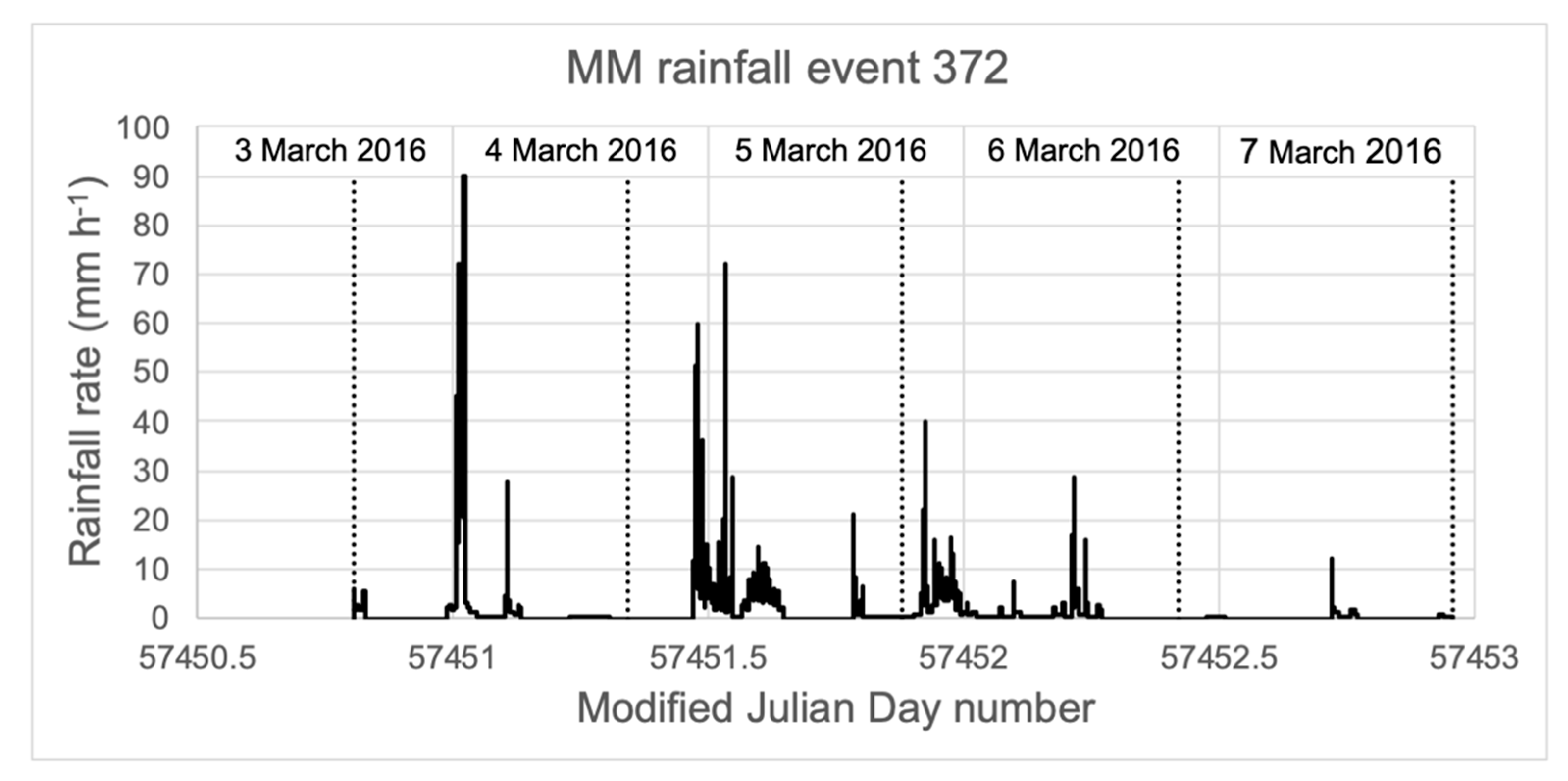
Figure 1 shows an intensity-time plot of MM rainfall event 372. This and the following diagrams (Figure 2 and Figure 3) are plotted from the intensity derived from each bucket tip event (Equation (1)) and thus involve no aggregation of the rainfall data. Though the most intense rain occurred in Q1, MM event 372 was classified as a 2Q event at a MIT = 360 min since more rainfall (26.2 mm) fell in Q2 than in Q1 (23.0 mm). The intensity bursts, separated by periods of intermittency, each fell wholly into a quartile without being divided across a quartile boundary. This appears to be a successful application of the Huff classification, though it highlights the propensity of this system to overlook intensity peaks.
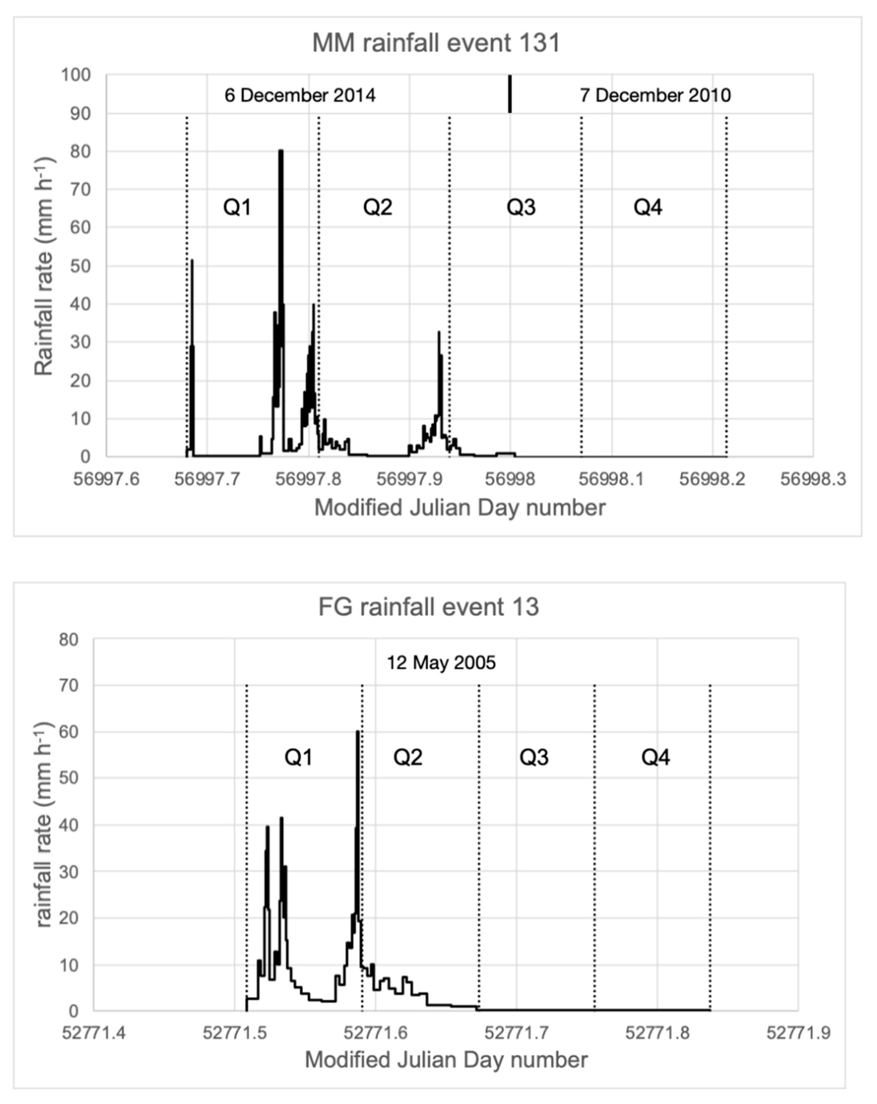
Two 1Q events that reveal different outcomes are shown in Figure 2. In both MM event 131 and FG event 13, intensity peaks are intersected by quartile boundaries so that the rain they delivered is divided among two quartiles in a manner that is entirely a consequence of the duration of the quartiles. In MM event 131, this happens twice, affecting the intensity peaks that are subdivided across the Q1–Q2 and the Q2–Q3 boundary.
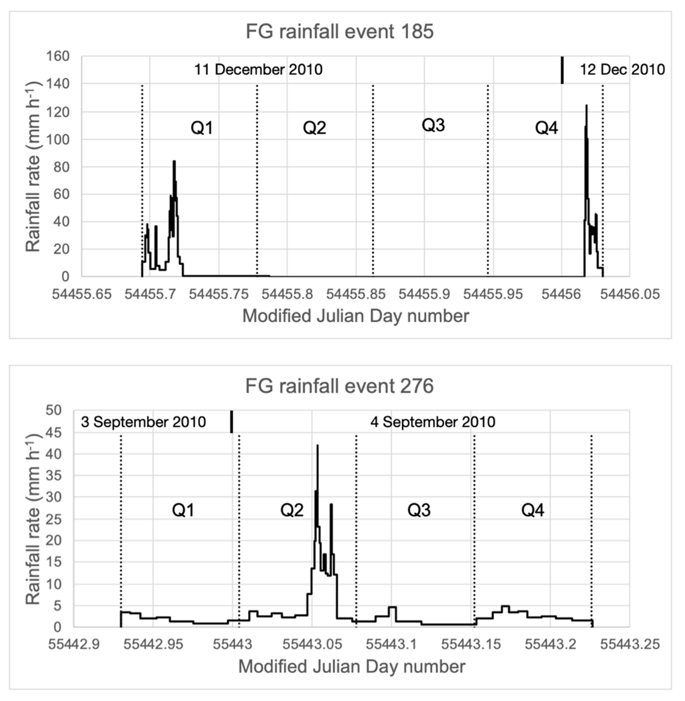
Two additional examples (Figure 3) show typical outcomes when isolated intensity peaks occur wholly within quartiles. FG event 185 contained intensity bursts in Q1 and Q4. Despite the peak in Q4 being the more intense, the event was classified as 1Q for a MIT = 360 min. Whether this is appropriate for a classification of rainfall events in relation to overland flow or soil erosion is not clear, since the peak in Q4 was more intense and would have struck soil already wetted by the prior rainfall in Q1. Late-peaking events such as this are known to yield more runoff and less infiltration (see earlier discussion). However, in this event, Q2 and Q3 recorded just 0.5 mm of rainfall, and together amounted essentially to a period of ~ 4 h with almost no rainfall, during which time soil infiltrability could have recovered partially prior to the arrival of the Q4 intensity peak.
FG event 276 presented a clear 2Q event, containing a single intensity peak located in Q2, whilst the remainder of the event had continuous but low-intensity rainfall (average intensity of the event was 2.95 mm h−1). For events having this kind of IP, the Huff classification appears to be applicable without difficulty.
3.4. Rainfall Intensities in the Quartiles
An important issue is how the rainfall rates in each quartile behave for changing values of the MIT criterion.
The results (Table 7) demonstrate that the quartile average rainfall rate in Q1 exceeded that of all other quartiles for both MM and FG and for all tested values of the MIT criterion. Likewise, the average rainfall rate in Q2 was in all cases the second-highest mean intensity. The situation for Q3 and Q4 was not consistent. For five of the seven MIT values at MM, the mean intensity of Q4 was the lowest, whilst in two cases, the lowest intensity occurred in Q3. At FG, again in five of the seven MIT values, Q4 had the lowest mean intensity, whilst in two cases, this occurred in Q3 and for different MIT values than the two cases at MM.
Maximum rainfall intensities recorded in a quartile may be said to reflect the occurrence of ‘intensity bursts’ [26], relatively short periods of rain but with a higher intensity than the remainder of the event. Maximum event intensity shows a different pattern to mean rainfall rate. At MM, for four MIT values, the most intense rainfall was recorded in Q2, with the other three occurring in Q1. At FG, six of the seven highest intensities occurred in Q1, and one occurred in Q3. Thus, whilst it is clear that Q1 has the highest mean rainfall intensities across all events at both MM and FG, the most intense rainfall within a single event often occurred in Q2 at MM, and once in Q3 at FG. However, there is a further factor that must be considered when comparing rainfall intensities in the various quartiles.
This factor is the effect of the absence of rainfall in Q2 and/or Q3 of some rainfall events, which contrasts with the always-present rainfall of all events in Q1 and Q4, by virtue of the process by which the events were delineated. Q1 and Q4 by definition always include at least one tip event. The MM and FG field sites differ in the proportion of no-rain in quartiles Q2 and Q3. It might be hypothesized that the chance for a no-rain quartile would be higher at MM, where rainfall events are considerably longer than at FG (Table 2 and Table 3). However, the reverse is the case, and the proportion of no-rain quartiles is actually higher at FG, at least for values of the MIT ≥ 360 min. For smaller values of the MIT (and the associated shorter events), the proportion of no-rain quartiles is lower at FG than at MM. Moreover, at MM, there is no clear dependence of the proportion of no-rain quartiles on the MIT. At FG, in contrast, that proportion rises monotonically for increasing values of the MIT, reaching a maximum of about 34% of events having no rain in either Q2 or Q3 for a MIT = 1440 min; at MM, the trend is less clear, but the corresponding value is smaller, at ~ 14% no-rain in Q2 and Q3 at a MIT = 1440 min (Table 8). Thus, once again, the difficult issue in relation to the use of the Huff classification is that the dependency of the occurrence of no-rain quartiles itself varies with the rainfall regime or climatology being analysed. As a result, so too does the rainfall depth and the mean intensity of the affected quartiles, with subsequent effects on the Huff quartile classification. Of course, when one or more quartiles records zero rainfall, only the remaining two or three quartiles can possibly be identified as the ‘dominant’ quartile. Thus, at FG (Table 6), the proportion of 4Q events increases with the MIT, but this is accompanied by an increasing proportion of zero-rain in both Q2 and Q3.
Eliminating these zero rainfall quartiles, which occur in Q2 and Q3 in up to about one-third of events, and averaging the rainfall intensity only for quartiles when rain was recorded, permits an estimate of the rainfall intensity when actually raining in the four quartiles to be made.
Results of this analysis (Table 7) show that eliminating the no-rain quartiles results in average rainfall rates in Q1 and Q2 that are much less different than when all data were included (Table 7). Nevertheless, for both MM and FG, and for all values of the MIT, Q1 showed the highest mean quartile rainfall rate. For all values of the MIT and at both MM and FG, the average intensities in Q4 remained the lowest among the quartiles. Likewise, in all cases the average intensity in Q2 exceeded that in Q3.
If we consider instead the maximum intensity, in some cases (for three values of the MIT at MM and one value at FG) the value was actually higher in Q2 than in Q1. This occurred for a MIT= 30 min, 60 min, and 240 min at MM, and for a MIT = 30 min at FG.
3.5. Are the Quartile Intensities Statistically Different When No-Rain Quartiles Are Excluded?
A t-test was applied to examine the hypothesis that after no-rain quartiles were eliminated, the differences in intensity between Q1 and Q2, and perhaps in some cases, Q3 and Q4, were too small to be of statistical significance.
Results show that at neither MM nor FG, nor for any value of the MIT, was the quartile mean intensity of Q1 statistically different from the quartile mean intensity of Q2 (results not shown). Moreover, at MM, the mean intensity of Q1 was not significantly different from the mean intensity of Q3 for values of a MIT = 120, 240, 360, 720, and 1440 min. At FG, the mean intensity of Q1 was not significantly different even from that of Q3 for a MIT = 360, 720, and 1440 min. Finally, at MM, for every value of the MIT, the mean intensity of Q1 was statistically different from the mean intensity of Q4. However, at FG even Q1 and Q4 mean intensities were not significantly different for a MIT = 720 and 1440 min. The difference was significant for all other values of the MIT there.
4. Discussion
The foregoing analysis has explored the influence of the MIT criterion employed to delineate rainfall events on the resulting Huff quartile classifications. Two principal results emerged.
The first result is that indeed, the Huff quartile classification exhibits a significant dependence on the MIT criterion. For instance, for MM and a MIT = 30 min, the Q1–Q4 percentages of events classified to each quartile were 33.7, 19.5, 18.3, and 28.4. For the same data, but using a MIT = 1440 min, the proportions changed to 38.3, 28.1, 25.0, and 9.4. Thus, the proportions of events classed as 1Q–3Q rose with the longer MIT, whilst the proportion of 4Q events fell to just 33% of the proportion using a MIT = 30 min. This is a notable change, 4Q events having been the second most frequent using a MIT = 30 min, but the least frequent, by a large margin, using a MIT = 1440. What can consequently be concluded about the Huff patterns of rainfall events at MM is unclear unless the MIT used in the delineation of the rainfall events is specified as a component of the Huff classification process.
There were similar changes in Huff quartile occurrences at FG (Table 6). There, the proportion of 4Q events rose by about 10% when the MIT criterion was increased from 30 min to 1440 min. Compensating changes occurred in 2Q and 3Q event proportions particularly.
The second conclusion is perhaps more significant because it may have more general implications for the application of the Huff quartile classification. It is that the influence of the MIT criterion on the resulting Huff quartile classifications was markedly different between the wet tropical site having generally long rainfall events (MM) and the dryland site (FG) having shorter and more intense events. The results (Table 5 and Table 6) showed that at MM with increasing MIT, 4Q events became more frequent and 2Q and 3Q events less frequent. The reverse applied to FG, where increasing MIT was associated with a decrease in the proportion of 4Q events, whilst 2Q and 3Q events tended to become more frequent.
The changed proportions of 4Q rainfall events are the most prominent effect of changing the MIT criterion. This is important, since 4Q events were shown to result in the largest proportion of rainfall becoming surface runoff (overland flow; [27,28,29], perhaps because in 4Q events the wettest quartile rainfall arrived on soil already wetted, and with an infiltrability that had consequently already been reduced by the prior rainfall in Q1–Q3. Whether 4Q events are the second most frequent or the least frequent (depending on the choice of MIT) at MM and FG, is therefore a major uncertainty that emerges when attempting to use the Huff quartile classification, since this change in relative quartile frequencies appears to depend on both the adopted value of the MIT and the rainfall climate or rainfall regime of the field location.
What Accounts for the Influence of the MIT on the Huff Quartile Classification?
What accounts for these changes in the proportions of the various quartiles, and especially of 4Q events, as the MIT criterion is changed, and simultaneously with the rainfall regime of the field location? The delineated rainfall events themselves change with the MIT, of course, tending to become longer and less intense for larger values of the MIT (Table 1 and Table 2). Given the complex IP of many rainfall events, the interaction of the MIT with the Huff quartile classification can be expected to be similarly complex, as separate showers of rain become grouped into longer events for larger MIT values or disaggregated for smaller MITs. However, the marked decline in the proportion of 4Q events at MM with increasing MIT suggests that the longer events show a decline in intensity through the course of the IP. In contrast, at FG, where the proportion of 4Q events increased with the MIT, the longer events must have had an increased intensity late in the IP. Here it is only possible to speculate on the influence of the precipitation mechanisms at the two field sites that might contribute to this, and this remains an area in need of further study.
At FG, rainfall events are shorter and more intense than at MM, reflecting the frequent occurrence of convective thunderstorm events that frequently arise on warm afternoons when the dryland surface has been warmed and drives thermally-driven uplift. Owing to the surface cooling that rapidly results when rain falls, and aided by evaporative cooling, the convective uplift in such events tends to wane quite rapidly, resulting in events lasting just a few hours. Therefore, when no-rain periods of up to 6 or 12 h are included when applying the larger MIT values, it may be that either a second, independent convective event (or perhaps a second mobile convective rain cell moving across the field observing site) becomes grouped with an earlier event to form a single, composite event, the second convective cell possibly resulting in a 4Q event, or an event where the Q4 intensity is little different from the Q1 intensity. This seems possible, since afternoon convection typically involves spatially scattered convective cells that can be carried in the direction of the steering winds. It is not uncommon for FG events to show early and late periods of rainfall separated by little or no rainfall (that is, intraevent intermittency).
In contrast, at MM, events tend to be prolonged, driven by continuous moisture advection consequent upon the sustained southeast trade winds, with uplift over the elevated terrain just inland. The resulting orographically enhanced rainfall consists of a continual sequence of showers that might have their origin in ‘bubbles’ of moist air that arises over the nearby warm ocean surface [30,31], and which continue as showers over the land. It is then possible that small values of the MIT are able to capture the IP of these individual showers that may involve a rising intensity as the convective uplift is boosted by the release of latent heat, thereby warming the atmosphere at cloud level and above. In contrast, the larger values of the MIT may result in the grouping of multiple showers embedded in the onshore winds (which may persist for one or more days) into longer events whose intensity wanes (yielding 1Q IPs and fewer 4Q events) as the synoptic pattern changes.
Apart from demonstrating a set of dependencies on the MIT and local rainfall regime, the present study has raised a number of procedural issues that bear on the application of Huff quartile classifications, in addition to their dependence on the choice of the MIT criterion.
First, when small values of the MIT are used (e.g., one or a few hours), relatively short rainfall events (and quartiles) with small rainfall depths are delineated. This increases the likelihood that one or more quartiles will record the same rainfall depth. Events with tied maximum rainfall depths in multiple quartiles cannot be classified using the Huff system. This was encountered frequently here, and it was resolved by using a random number selection to allocate tied events in an unbiassed way to one or the other of the tied quartiles in roughly equal numbers. This has the same effect as adding a negligible rainfall depth to one quartile at random but avoids any effect on the rainfall depths. After all, if we had higher precision in rainfall depth measurements (and in the timing of tip events which may only occur after much of the rain needed to fill the bucket has fallen at earlier moments, possibly in the preceding quartile), fewer ties would be likely to occur.
Second, in terms of the proportions of 1Q, 4Q, etc., rainfall events, there is an effect of the event delineation using the MIT approach. By definition, both Q1 and Q4 must record at least one tip event, and thus at least some rainfall. In contrast, Q2 and Q3 can and do on occasion record no rainfall. By itself, this means that it is probable that the frequency of 1Q and 4Q events will exceed that of 2Q and 3Q events. Likewise, this effect may result in rainfall intensities appearing to be higher in Q1 and Q4, simply because these quartiles never record zero rainfall. The unadjusted event frequencies do not reflect only the rainfall mechanisms delivering rain during the course of the event, but also reflect in part the arbitrary process of event and quartile delineation and its interaction with true rainfall intermittency [32].
Third, a consequence of the effect just mentioned, the intensities of Q2 and Q3 (which occasionally record no rainfall) tend to be lower than the intensity of Q1 and Q4, which never record zero rainfall depths. Again, this does not usefully reflect rainfall mechanisms, but rather is an artefact of the data processing. It is influenced by the choice of the MIT. This was examined further here by analysing the intensity from only those quartiles when rain was recorded in an attempt to quantify more appropriately the intensity when actually raining during the four quartiles. As was seen in Table 8, at both MM and FG, larger MIT values result in a larger proportion of Q2 and Q3 quartiles having no rainfall. This effect is larger at FG, reaching 34–35% of Q2 and Q3 quartiles for a MIT = 1440 min, so that the effect is far from negligible. Nevertheless, in many cases, the mean intensity in Q1 is not statistically different from the mean intensity in other quartiles, including in some cases even Q4.
Fourth, given that rainfall event durations can take any value, the durations of quartiles can thus take any value. For instance, a rainfall event lasting 3 h 37 min has quartile durations of 54.25 min. Accurately tallying the rainfall recorded in such quartiles clearly requires high temporal resolution in the rainfall data. Hourly rainfall totals are insufficient, and even 15-min rainfalls provide too little resolution to reliably allocate the rain to a quartile. A lack of sufficient resolution must result in uncertainty about the actual rainfall in quartiles such as the one just mentioned, whose duration is not a multiple of whole clock hours. This casts doubt on the reliability of the identification of the ‘dominant’ quartile for Huff classification purposes when hourly or other time-aggregated data are used.
In light of the foregoing, it has to be considered that, as a means of categorising the IP of rainfall events, the Huff quartile system suffers from multiple challenges that cast doubt on the utility of the results obtained. A fundamental concern raised by Huff (1967 [3]) was that his Illinois rainfall data confirmed that most of the rain that is recorded in an event often falls in just a small part of the overall duration, regardless of the length of the event. Given that the locations of the quartile boundaries are set independently of the timing of the more intense ‘showers’ or ‘bursts’ of rain that are separated by less rainy periods within an event, there is a good chance that a quartile boundary will split a burst between two quartiles. In this way, the timing of the burst arrival is blurred because it affects the apparent intensity in two quartiles. Figure 2 illustrates this phenomenon. It is evident in both plots in Figure 2 that quartile boundaries occur within bursts of rainfall, such that some rain is allocated to the earlier quartile and some to the subsequent one. This will sometimes occur and sometimes not—and will presumably be more complex or occur more frequently in multipeaked rainfall events. It would be worthwhile to study a large sample of high-resolution IPs of recorded rainfall events to find the extent of this occurrence. It may also be advantageous to explore the use of an intensity threshold, rather than tallying all rainfall data regardless of its intensity, in allocating events to a particular Huff quartile.
The frequent lack of a statistical difference in quartile means rainfall rates for a field, a hillslope, or a catchment etc., through a series of rainfall events might each have an identifiable quartile Huff classification. The sequence of rainfall events through a period of years exposes the landscape to events of all dominant Huff quartiles, such that their aggregate or cumulative effect is perhaps of greater significance for landscape processes than is any single event. This requires further investigation. However, because in almost all cases analysed here, mean Q1 intensities were statistically different from mean Q4 intensities (often being considerably higher), but not from Q2 or Q3 intensities, it seems reasonable to speculate that the proportions of 1Q and 4Q events at a particular site may well have importance for landscape processes, with 2Q and 3Q events having a lesser level of importance.
5. Conclusions
The classification of rainfall events according to the Huff quartile system has been widely adopted since the original work of Huff (1967) [3], who sought to describe the IP in a way that was relevant to the occurrence of flooding, soil erosion, and other processes. He stressed the importance of the time within a rainfall event when the most rain was recorded, typically in the first quartile, and less commonly in the other three quartiles. The Huff classification continues to be widely used, notably for storm modelling purposes, but also as a guide to the IP that needs to be reproduced in rainfall simulation experiments designed to be relevant and appropriate at a particular research location.
The present study has shown that the Huff quartile classification depends on the value of the MIT criterion that is adopted to delineate separate rainfall events. Huff (1967) [3] used 6 h, but many other values are in use. The results presented here demonstrate that the Huff classification changes if the value of the MIT changes. Moreover, the amount and direction of the change depends on the rainfall regime or climatology of the study location. This was shown here by very different effects of changing the MIT in a very wet tropical environment having long rainfall events and a dryland location typified by short, more intense, convective events. Therefore, it cannot be claimed that the Huff classification actually describes the rainfall events at a place; rather, it presents a particular view of those rainfall events that is strongly dependent on the choice of the MIT and its interaction with the local rainfall regime. This occurs through the effects of factors such as the rainfall event duration—such as the long events at MM but the much shorter ones at FG. It is evidently inappropriate to apply the same MIT to these two very different locations, and, by implication, the same can be expected to apply at other locations and in other climates. Very large changes in the proportions, especially of 4Q events, were reported here from the MM data, for example, between a MIT = 30 min and a MIT = 1440 min data. This clearly leaves the question of whether 4Q events are relatively common or uncommon at MM unresolved. The answer depends on which MIT is used to delineate the rainfall events. This is not a very satisfactory situation. The major conclusion from this study is therefore that the conventional Huff quartile classification, if applied with the 6 h MIT that Huff adopted as being appropriate for the eastern USA, will lead to inappropriate and potentially misleading results if incautiously applied in other locations that have different rainfall regimes.
A partial solution to this problem is to focus on metric measures of the quartiles, such as the mean intensity and the maximum intensity of the rainfall. For MM, a MIT = 30 min, for instance, showed that the most intense rainfall occurred in Q2, not Q1.
In light of the results presented here, it is considered that careful thought should be given to whether the Huff quartile classification is actually an appropriate and meaningful tool for the classification and description of rainfall events, depending on the specific purpose for which the classification is intended. At a minimum, the dependency on the MIT criterion and on the local rainfall regime should be acknowledged and, if possible, quantified. Only in this way will we learn more about these dependencies and their magnitude in different locations and be able to consider ways to accommodate or allow for them.
Funding
This research received no external funding.
Institutional Review Board Statement
Not applicable.
Informed Consent Statement
Not applicable.
Data Availability Statement
Not applicable.
Conflicts of Interest
The author declares no conflict of interest.
References
- Wartalska, K.; Kaźmierczak, B.; Nowakowska, M.; Kotowski, A. Analysis of Hyetographs for Drainage System Modeling. Water 2020, 12, 149. [Google Scholar] [CrossRef] [Green Version]
- Horner, W.W.; Jens, S.W. Surface Runoff Determination from Rainfall without Using Coefficients. Trans. Am. Soc. Civ. Eng. 1942, 107, 1039–1075. [Google Scholar] [CrossRef]
- Huff, F.A. Time distribution of rainfall in heavy storms. Water Resour. Res. 1967, 3, 1007–1019. [Google Scholar] [CrossRef]
- Yin, S.; Xie, Y.; Nearing, M.A.; Guo, W.; Zhu, Z. Intra-storm temporal patterns of rainfall in China using Huff curves. Trans. Am. Soc. Agric. Biol. Eng. 2016, 59, 1619–1632. [Google Scholar]
- Pan, C.; Wang, X.; Liu, L.; Huang, H.; Wang, D. Improvement to the Huff Curve for Design Storms and Urban Flooding Simulations in Guangzhou, China. Water 2017, 9, 411. [Google Scholar] [CrossRef] [Green Version]
- Back, Á.J.; Rodrigues, M.L.G. Characterization of temporal rainfall distribution in Florianópolis, Santa Catarina, Brazil. Rev. Bras. Climatol. 2021, 28, 17. [Google Scholar] [CrossRef]
- Xiong, J.; Tang, C.; Gong, L.; Chen, M. Variability of rainfall time distributions and their impact on peak discharge in the Wenchuan County, China. Bull. Eng. Geol. Environ. 2021, 80, 7113–7129. [Google Scholar] [CrossRef]
- El-Sayed, E.A.H. Development of synthetic rainfall distribution curves for Sinai area. Ain Shams Eng. J. 2018, 9, 1949–1957. [Google Scholar] [CrossRef]
- An, J.; Zhang, Y.; Wang, Y. Rainstorm pattern effects on the size distribution of soil aggregate in eroded sediment within contour ridge systems. J. Soils Sediments 2020, 20, 2192–2206. [Google Scholar] [CrossRef]
- Zeimetz, F.; Schaefli, B.; Artigue, G.; Hernández, J.G.; Schleiss, A.J. Swiss Rainfall Mass Curves and their Influence on Extreme Flood Simulation. Water Resour. Manag. 2018, 32, 2625–2638. [Google Scholar] [CrossRef]
- Adams, B.J.; Fraser, H.G.; Howard, C.D.D.; Hanafy, M.S. Meteorological Data Analysis for Drainage System Design. J. Environ. Eng. 1986, 112, 827–848. [Google Scholar] [CrossRef]
- Bonta, J.V.; Shahalam, A. Cumulative storm rainfall distributions: Comparison of Huff curves. J. Hydrol. 2003, 42, 65–74. [Google Scholar]
- Bonta, J.V. Development and utility of Huff curves for disaggregating precipitation amounts. Appl. Eng. Agric. 2004, 20, 641–656. [Google Scholar] [CrossRef]
- Dunkerley, D. Identifying individual rain events from pluviograph records: A review with analysis of data from an Australian dryland site. Hydrol. Process. 2008, 22, 5024–5036. [Google Scholar] [CrossRef]
- Coutinho, J.V.; Almeida, C.D.N.; Leal, A.M.F.; Barbosa, L.R. Characterization of sub-daily rainfall properties in three raingauges located in northeast Brazil. Proc. Int. Assoc. Hydrol. Sci. 2014, 364, 345–350. [Google Scholar] [CrossRef]
- Wang, W.; Yin, S.; Xie, Y.; Nearing, M.A. Minimum Inter-Event Times for Rainfall in the Eastern Monsoon Region of China. Trans. ASABE 2019, 62, 9–18. [Google Scholar] [CrossRef] [Green Version]
- Joo, J.; Lee, J.; Kim, J.H.; Jun, H.; Jo, D. Inter-Event Time Definition Setting Procedure for Urban Drainage Systems. Water 2013, 6, 45–58. [Google Scholar] [CrossRef] [Green Version]
- Paoletti, A.; Becciu, G.; Sanfilippo, U. Filling and emptying cycles for stormwater storage tanks in separated systems. In Proceedings of the 6th International Conference on Sustainable Techniques and Strategies for Urban Water Management, Lyon, France, 25–28 June 2007. [Google Scholar]
- Pérez-Arellano, R.; Moreno-Pérez, M.; Roldán-Cañas, J. Estimation of canopy drying time after rainfall using leaf wetness sensor in Pinus pinea in a Mediterranean forest in Córdoba, Spain. Geophys. Res. Abstr. 2016, 18, EGU2016-4883. [Google Scholar]
- Driscoll, E.D.; Palhegyi, G.E.; Strecker, E.W.; Shelley, P.E. Analysis of Storm Event Characteristics for Selected Rainfall Gages throughout the United States; U.S. Environmental Protection Agency: Oakland, CA, USA, 1989; p. 43.
- Pui, A.; Sharma, A.; Santoso, A.; Westra, S. Impact of the El Niño–Southern Oscillation, Indian Ocean Dipole, and Southern Annular Mode on Daily to Subdaily Rainfall Characteristics in East Australia. Mon. Weather Rev. 2012, 140, 1665–1682. [Google Scholar] [CrossRef] [Green Version]
- Carbone, M.; Turco, M.; Brunetti, G.; Piro, P. A Cumulative Rainfall Function for Subhourly Design Storm in Mediterranean Urban Areas. Adv. Meteorol. 2015, 2015, 528564. [Google Scholar] [CrossRef] [Green Version]
- Chin, R.J.; Lai, S.H.; Chang, K.B.; Jaafar, W.Z.W.; Othman, F. Relationship between minimum inter-event time and the number of rainfall events in Peninsular Malaysia. Weather 2016, 71, 213–218. [Google Scholar] [CrossRef]
- Medina-Cobo, M.T.; García-Marín, A.; Estévez, J.; Ayuso-Muñoz, J. The identification of an appropriate Minimum Inter-event Time (MIT) based on multifractal characterization of rainfall data series. Hydrol. Process. 2016, 30, 3507–3517. [Google Scholar] [CrossRef]
- Othman, M.A.; A Ghani, A. Distribution of rainfall events in northern region of Peninsular Malaysia. IOP Conf. Ser. Earth Environ. Sci. 2020, 476. [Google Scholar] [CrossRef]
- Dunkerley, D.L. Rainfall intensity bursts and the erosion of soils: An analysis highlighting the need for high temporal resolution rainfall data for research under current and future climates. Earth Surf. Dyn. 2019, 7, 345–360. [Google Scholar] [CrossRef] [Green Version]
- Dunkerley, D. An approach to analysing plot scale infiltration and runoff responses to rainfall of fluctuating intensity. Hydrol. Process. 2016, 31, 191–206. [Google Scholar] [CrossRef]
- Zhai, X.; Guo, L.; Liu, R.; Zhang, Y. Rainfall threshold determination for flash flood warning in mountainous catchments with consideration of antecedent soil moisture and rainfall pattern. Nat. Hazards 2018, 94, 605–625. [Google Scholar] [CrossRef]
- Ran, Q.; Wang, F.; Gao, J. Modelling Effects of Rainfall Patterns on Runoff Generation and Soil Erosion Processes on Slopes. Water 2019, 11, 2221. [Google Scholar] [CrossRef] [Green Version]
- Woodcock, A.H. The Origin of Trade-Wind Orographic Shower Rains. Tellus 1960, 12, 315–326. [Google Scholar] [CrossRef]
- Connor, G.J.; Bonell, M. Air mass and dynamic parameters affecting trade wind precipitation on the northeast Queensland tropical coast. Int. J. Clim. 1998, 18, 1357–1372. [Google Scholar] [CrossRef]
- Dunkerley, D. How does sub-hourly rainfall intermittency bias the climatology of hourly and daily rainfalls? Examples from arid and wet tropical Australia. Int. J. Clim. 2018, 39, 2412–2421. [Google Scholar] [CrossRef]
Figure 1.
Intensity–time plot of MM rainfall event 372. Event duration was 51.7 h, depth 69.2 mm, and event mean intensity 1.3 mm h−1. The peak intensity in each quartile appears to decline as the event progresses, from a peak of 90 mm h−1 in Q1. Nevertheless, this was classified as a 2Q event for a MIT = 360 min. Note that the multiple intensity bursts each fall wholly within a quartile, and none is split across a quartile boundary (shown by dotted vertical lines). Gregorian dates are marked across the top of the panel, spanning five days in March 2016. See text for additional commentary.

Figure 2.
Intensity–time plots for MM rainfall event 131 (upper) and FG rainfall event 13 (lower). MM 131 had a duration of 12.8 h and delivered 27.8 mm at a mean rainfall rate of 2.2 mm h−1. FG 13 had a duration of 7.9 h and delivered 27.0 mm at a mean rainfall rate of 3.4 mm h−1. Both events were classified as 1Q for a MIT = 360 min. However, both contained intensity bursts that were split between two quartiles, which occurred twice in MM 131 and once in FG 13. Quartile boundaries are shown by dotted vertical lines. Gregorian dates are shown at the top of each panel, and the heavy vertical bar in the upper panel marks midnight on December 6. See text for additional commentary.

Figure 3.
Intensity–time plots of FG rainfall event 185 (upper) and FG rainfall event 276 (lower). FG 185 had a duration of 8.05 h and delivered 27.0 mm at a mean rainfall rate of 3.35 mm h−1. FG 276 had a duration of 7.1 h and delivered 21 mm at a mean rainfall rate of 2.95 mm h−1. The intensity peaks fall wholly within separate quartiles. FG event 185 displays a common IP in which early Q1 rain is followed by a period of intermittency until late Q4 rain. Quartile boundaries are shown by dotted vertical lines. Gregorian dates are shown at the top of each panel, and the heavy vertical line between days marks midnight. See text for additional commentary.


Table 1.
Properties of rainfall events at the MM observing site for the seven different values of the MIT criterion.
Table 1.
Properties of rainfall events at the MM observing site for the seven different values of the MIT criterion.
| MIT (Min) | N Events (>1 Tip Event) | Mean Quartile Duration (h) | Mean Event Duration (h) | Mean Event Depth (mm) | Mean Event Intensity (mm h−1) |
|---|---|---|---|---|---|
| 30 | 2664 | 0.25 | 0.99 | 3.43 | 4.92 |
| 60 | 1636 | 0.6 | 2.40 | 5.59 | 3.79 |
| 120 | 936 | 1.47 | 5.87 | 9.77 | 3.08 |
| 240 | 544 | 3.28 | 13.11 | 16.82 | 2.29 |
| 360 | 427 | 4.77 | 19.07 | 21.42 | 2.22 |
| 720 | 263 | 9.67 | 38.66 | 34.78 | 1.61 |
| 1440 | 163 | 20.32 | 81.29 | 56.12 | 0.87 |
Table 2.
Properties of rainfall events at the FG observing site for the seven different values of the MIT criterion.
Table 2.
Properties of rainfall events at the FG observing site for the seven different values of the MIT criterion.
| MIT (Min) | N Events (>1 Tip Event) | Mean Quartile Duration (h) | Mean Event Duration (h) | Mean Event Depth (mm) | Mean Event Intensity (mm h−1) |
|---|---|---|---|---|---|
| 30 | 465 | 0.24 | 0.96 | 5.76 | 8.85 |
| 60 | 383 | 0.41 | 1.63 | 6.99 | 7.54 |
| 120 | 328 | 0.63 | 2.51 | 8.16 | 6.11 |
| 240 | 292 | 0.92 | 3.69 | 9.17 | 4.89 |
| 360 | 262 | 1.28 | 5.13 | 10.22 | 4.32 |
| 720 | 238 | 1.96 | 7.82 | 11.25 | 3.96 |
| 1440 | 208 | 3.14 | 12.56 | 12.87 | 3.24 |
Table 3.
Properties of the rainfall events employed in Huff quartile classification at the MM observing site, for the seven different values of the MIT criterion.
Table 3.
Properties of the rainfall events employed in Huff quartile classification at the MM observing site, for the seven different values of the MIT criterion.
| MIT (Min) | N Events | Mean Quartile Duration (h) | Mean Event Duration (h) | Mean Event Depth (mm) | Mean Event Intensity (mm h−1) |
|---|---|---|---|---|---|
| 30 | 1308 | 0.43 | 1.71 | 5.80 | 4.69 |
| 60 | 939 | 0.95 | 3.82 | 8.79 | 3.54 |
| 120 | 607 | 2.14 | 8.55 | 14.27 | 2.84 |
| 240 | 391 | 4.40 | 17.60 | 22.69 | 2.08 |
| 360 | 322 | 6.09 | 24.36 | 27.76 | 2.03 |
| 720 | 216 | 11.38 | 45.50 | 41.36 | 1.71 |
| 1440 | 129 | 24.31 | 97.24 | 68.97 | 0.82 |
Table 4.
Properties of the rainfall events employed in Huff quartile classification at the FG observing site, for the seven different values of the MIT criterion.
Table 4.
Properties of the rainfall events employed in Huff quartile classification at the FG observing site, for the seven different values of the MIT criterion.
| MIT (Min) | N Events | Mean Quartile Duration (h) | Mean Event Duration (h) | Mean Event Depth (mm) | Mean Event Intensity (mm h−1) |
|---|---|---|---|---|---|
| 30 | 222 | 0.39 | 1.58 | 9.43 | 10.29 |
| 60 | 212 | 0.63 | 2.50 | 10.81 | 8.23 |
| 120 | 196 | 0.91 | 3.62 | 12.19 | 6.83 |
| 240 | 184 | 1.25 | 4.98 | 13.31 | 5.77 |
| 360 | 170 | 1.70 | 6.81 | 14.59 | 5.14 |
| 720 | 158 | 2.57 | 10.27 | 15.94 | 4.68 |
| 1440 | 144 | 4.07 | 16.26 | 17.69 | 3.74 |
Table 5.
Huff quartile classifications for rainfall events at MM for seven different values of the MIT criterion.
Table 5.
Huff quartile classifications for rainfall events at MM for seven different values of the MIT criterion.
| MIT (Min) | N Events | % 1Q | % Q2 | % 3Q | % 4Q |
|---|---|---|---|---|---|
| 30 | 1308 | 33.7 | 19.5 | 18.3 | 28.4 |
| 60 | 939 | 33.9 | 20.3 | 17.8 | 27.0 |
| 120 | 607 | 31.9 | 25.5 | 19.1 | 23.4 |
| 240 | 391 | 32.5 | 27.1 | 20.2 | 20.2 |
| 360 | 322 | 36.2 | 25.4 | 19.2 | 19.2 |
| 720 | 216 | 40.3 | 22.7 | 20.8 | 16.2 |
| 1440 | 129 | 38.3 | 28.1 | 25.0 | 9.4 |
Table 6.
Huff quartile classifications for rainfall events at FG for seven different values of the MIT criterion.
Table 6.
Huff quartile classifications for rainfall events at FG for seven different values of the MIT criterion.
| MIT (Min) | N Events | % 1Q | % Q2 | % 3Q | % 4Q |
|---|---|---|---|---|---|
| 30 | 222 | 39.6 | 19.4 | 22.5 | 18.5 |
| 60 | 212 | 39.2 | 20.8 | 17.4 | 22.6 |
| 120 | 196 | 43.9 | 18.4 | 18.4 | 19.4 |
| 240 | 184 | 39.7 | 17.9 | 18.5 | 23.9 |
| 360 | 170 | 38.2 | 18.8 | 19.4 | 23.5 |
| 720 | 158 | 40.5 | 17.1 | 17.1 | 24.7 |
| 1440 | 144 | 38.2 | 14.6 | 18.1 | 29.2 |
Table 7.
Mean rainfall rates (in mm h−1) for each quartile at MM and FG, for all seven values of the MIT criterion. For Q2 and Q3 and for each MIT, the unadjusted mean rainfall rate is listed first, followed by the higher, adjusted value (not including zero-rain quartiles) in parentheses. At a MIT = 1440 min, the difference reaches almost 2.0 mm h−1 for Q2 at FG, or an increase in the mean quartile rainfall rate of 50%. This makes the quartile mean intensity higher in Q2 than in Q1.
| Field Site: | MM | FG | ||||||
|---|---|---|---|---|---|---|---|---|
| MIT (Min) | Q1 | Q2 | Q3 | Q4 | Q1 | Q2 | Q3 | Q4 |
| 30 | 5.8 | 4.6 (5.2) | 4.0 (4.6) | 4.3 | 13.7 | 11.2 (11.6) | 8.6 (9.3) | 7.6 |
| 60 | 4.4 | 3.2 (4.3) | 2.9 (3.5) | 3.1 | 11.9 | 8.9 (9.7) | 6.1 (7.0) | 5.9 |
| 120 | 3.5 | 3.0 (3.5) | 2.5 (2.9) | 2.3 | 10.3 | 7.1 (7.9) | 5.1 (6.0) | 4.8 |
| 240 | 2.8 | 2.3 (2.8) | 1.7 (2.0) | 1.5 | 8.6 | 5.9 (7.0) | 4.2 (5.0) | 4.4 |
| 360 | 2.9 | 2.2 (2.5) | 1.7 (1.9) | 1.3 | 7.4 | 5.3 (6.9) | 3.8 (4.9) | 4.0 |
| 720 | 2.5 | 1.9 (2.4) | 1.5 (1.7) | 0.9 | 6.7 | 4.9 (6.3) | 3.6 (5.0) | 3.5 |
| 1440 | 1.1 | 0.9 (1.1) | 0.8 (0.9) | 0.5 | 5.0 | 3.7 (5.7) | 3.1 (4.8) | 3.0 |
Table 8.
Proportion of quartiles Q2 and Q3 recording zero rainfall, at both MM and FG, for all seven values of the MIT criterion. Note that at FG, events defined using small values of the MIT have few no-rain quartiles, whilst events defined using large values of the MIT have larger proportions of no-rain quartiles, the proportions for both Q2 and Q3 exceeding one-third of all events for a MIT = 1440 min.
| MIT (Min) | N Events | % 1Q | % Q2 | % 3Q | % 4Q |
|---|---|---|---|---|---|
| 30 | 222 | 39.6 | 19.4 | 22.5 | 18.5 |
| 60 | 212 | 39.2 | 20.8 | 17.4 | 22.6 |
| 120 | 196 | 43.9 | 18.4 | 18.4 | 19.4 |
| 240 | 184 | 39.7 | 17.9 | 18.5 | 23.9 |
| 360 | 170 | 38.2 | 18.8 | 19.4 | 23.5 |
| 720 | 158 | 40.5 | 17.1 | 17.1 | 24.7 |
| 1440 | 144 | 38.2 | 14.6 | 18.1 | 29.2 |
Publisher’s Note: MDPI stays neutral with regard to jurisdictional claims in published maps and institutional affiliations. |
© 2022 by the author. Licensee MDPI, Basel, Switzerland. This article is an open access article distributed under the terms and conditions of the Creative Commons Attribution (CC BY) license (https://creativecommons.org/licenses/by/4.0/).
Share and Cite
MDPI and ACS Style
Dunkerley, D. Regional Rainfall Regimes Affect the Sensitivity of the Huff Quartile Classification to the Method of Event Delineation. Water 2022, 14, 1047. https://doi.org/10.3390/w14071047
AMA Style
Dunkerley D. Regional Rainfall Regimes Affect the Sensitivity of the Huff Quartile Classification to the Method of Event Delineation. Water. 2022; 14(7):1047. https://doi.org/10.3390/w14071047
Chicago/Turabian StyleDunkerley, David. 2022. "Regional Rainfall Regimes Affect the Sensitivity of the Huff Quartile Classification to the Method of Event Delineation" Water 14, no. 7: 1047. https://doi.org/10.3390/w14071047
Note that from the first issue of 2016, this journal uses article numbers instead of page numbers. See further details here.