A Comprehensive View of the ASM1 Dynamic Model: Study on a Practical Case

Abstract

The ASM1 model was elaborated by the IWA Task Group for Mathematical Modelling, with the aim of explaining and predicting the output values of organic matter concentration in activated sludge processes, especially for domestic wastewaters. In recent years, ASM1 has been completed with new components and extended to other biological processes, including biological membrane reactors, activated carbon filters, and microalgae bioreactors. In this article, the essentials of this model are studied by outlining the original topics that were formulated in the model, and by using a practical example of a wastewater treatment plant (WWTP), which can clarify the application of the ASM1. A protocol of approximation between the dynamic model and the experimental data for the COD effluent concentration is presented, based on three steps of tuning and fine tuning, and the corrected values of the kinetic parameters Y_H and μ_H,max are calculated in accordance with the minimum error. In the simulation procedure, the baseline and dynamism are controlled, comparing them to the experimental data line, and the values obtained for the kinetic parameters are Y_H = 0.60 and μ_H,max = 0.40 d⁻¹. The kinetic parameters reflect the activity of the mixed community of microorganisms in the WWTP.

1. Introduction

Biological wastewater treatment is strongly influenced by environmental perturbations. Variations in temperature, influent organic matter, biomass concentration, and influent flow modify the bacterial community activity and produce a modification in the output concentration of the organic matter. Traditional stationary mathematical models do not consider this situation, which occurs daily in wastewater treatment plants (WWTP).

A dynamic model is a non-stationary mathematical model, which considers the dynamic behaviour of the variables affecting the output parameters. The IWA Task Group for Mathematical Modelling (International Water Association), conducted by Morgens Henze, published the first activated sludge model (ASM1) [1] in 1987, which is a deterministic model (based on basic engineering principles), initially formulated as a general mass balance to the biological reactor. This original model was extended to phosphorus and nitrogen removal, oxygen consumption, and sludge production [2,3,4]. All ASMs are recorded in the IWA Report No. 9 [5].

The ASM1 includes 13 components (different types of substrates and biomass) and 8 fundamental processes (growth and substrate utilisation rates), resulting, initially, in 13 mass balance equations, with almost 20 kinetic parameters. The model was initially proposed for domestic wastewater, and was validated more than a decade ago in its application to specific cases of WWTPs [6,7]. The ASM1 is often too complicated for solving predictions in real-scale operations at wastewater treatment plants. The characterisation of wastewater for mathematical modelling with the ASM1 can sometimes be hard and time consuming. In addition, the use of so many parameters for the model can result in poor parameter identifiability [8].

The ASM1 was designed to be adapted to the special characteristics of the wastewater and the biological treatments applied. In other words, the system of differential equations is limited to the components in consideration, and the process rates are selected as a function of the biological treatment conditions.

In recent years, the ASM1 has been improved by including new components or processes to the original model [9,10], because of the special and flexible configuration of the ASM1, which permits continuous updates and adjustments. The application of this dynamic model is not only possible for activated sludge processes [11,12,13,14], but also for other biological treatments, such as membrane bioreactors [15,16] and microalgae systems [17]. In fact, the ASM1 represents the basis for the formulation of new mathematical models for nutrient removal in WWTPs [18] and in granular activated carbon filters [19], and for the application of activated sludge models (ASMs) to MBR systems [20,21].

The ASM1 has been applied to diverse biological processes, for suspension growth or fixed growth, for bacteria or microalgae, but the detailed procedure of formulating the model, related to the election of components and processes, and especially to the protocol of simulation, has not been described in depth, and needs an explanation for more extended use, mainly in WWTPs. Predicting the COD value in a WWTP under abnormal situations or special environmental events is of great value for adequate correction of the effluents, and for preserving the quality of natural streams.

In the present work, the ASM1 will be described in depth, and, as a novelty, a protocol of simulation, based on the approximation between the dynamic model and real data (tuning), will be proposed. A simulation of the output COD concentration will be performed from a medium–high-sized WWTP (260,000 habitants), considering dynamism in the reactor temperature (affecting μ_H), biomass concentration, and influent COD. The effect of dynamic variables on the output parameter (COD) will be analysed from the biological treatment point of view, explaining the behaviour of the bacterial community, focusing on the response to organic matter removal.

2. Materials and Methods

2.1. Dynamic Model ASM1

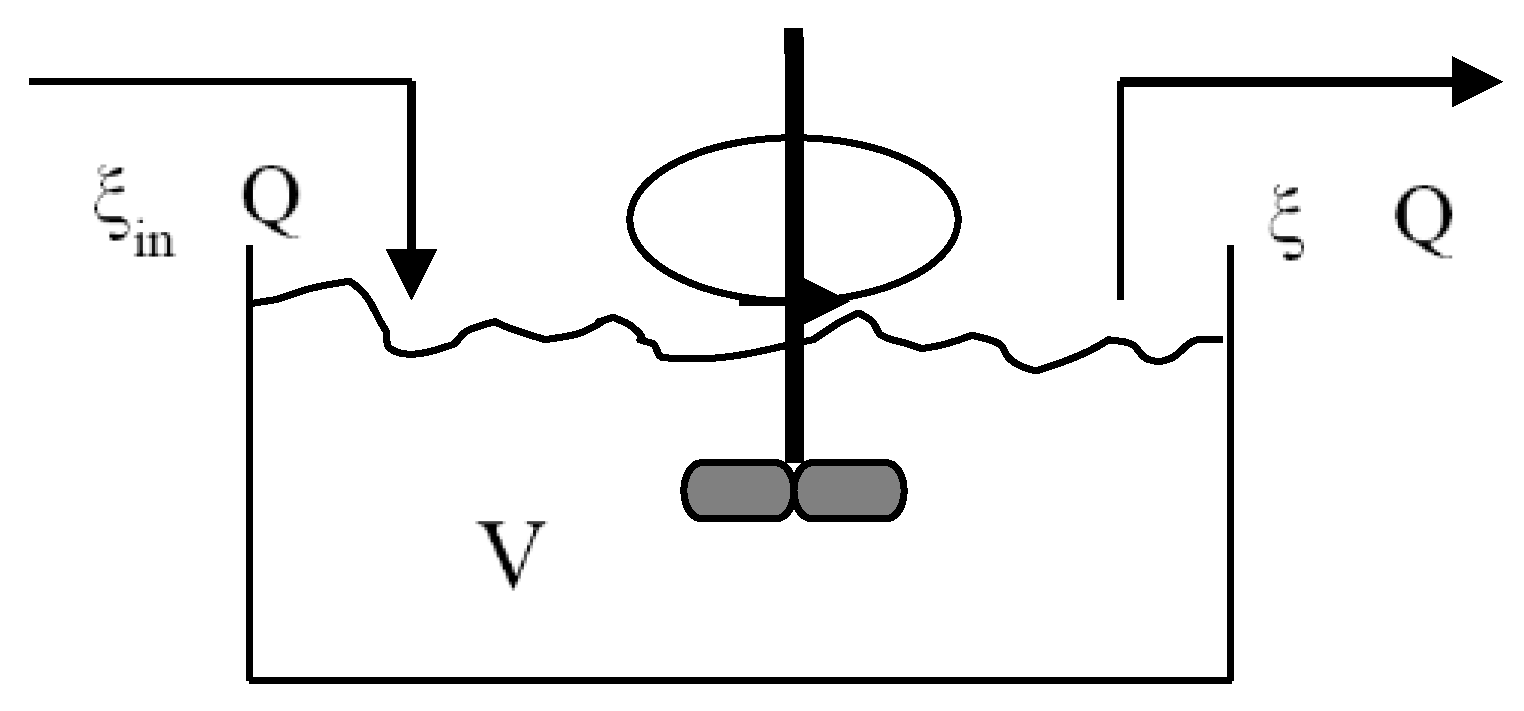
The mathematical expression for the generic mass balance applied to the vector ξ, representing substrate or biomass concentration, is as follows (Figure 1):

$$V\frac{d\xi }{dt}=Q{\xi }_{in}-Q\xi +Vr\left(\xi \right)$$

(1)

$$\frac{d\xi }{dt}=r\left(\xi \right)+\frac{1}{\Theta }\left({\xi }_{in}-\xi \right)$$

(2)

where Θ in Equation (2) is the hydraulic residence time (HRT) and r(ξ) is the conversion vector of the variable ξ (substrate utilisation global rate).

The substrate utilisation global rate (r_i) in the ASM1 is a conversion rate for the component i by the process j, as follows:

$$r_i={\displaystyle \sum }_j{\nu }_{ij}{\rho }_j$$

(3)

where ν_ij is the stoichiometric coefficient and ρ_j is the process rate. This equation defines a differential equation system, in which every differential equation has the form of Equation (2) for each component i of the model, affected by the different process rates designed by the j subscript. The process rates that affect the components of the ASM1 are described in the Peterson matrix (

Table 1. Peterson matrix for the ASM1. Components are recorded in columns and processes can be identified in rows.

i—Component→ j—Process↓	1 SI	2 SS	3 XI	4 XS	5 XBH	6 XBA	7 XP	8 SO	9 SNO	10 SNH	11 SND	12 XND	13 SALK
1-Aerobic growth of heterotrophs		$-\frac{1}{Y_H}$			1			$-\frac{1-Y_H}{Y_H}$		−iXB			$\frac{-i_{XB}}{14}$
2-Anoxic growth of heterotrophs		$-\frac{1}{Y_H}$			1				$-\frac{1-Y_H}{2.86Y_H}$	−iXB			$\frac{1-Y_H}{14\times 2.86Y_H}-\frac{i_{XB}}{14}$
3-Aerobic growth of autotrophs						1		$-\frac{4.57-Y_A}{Y_A}$	$\frac{1}{Y_A}$	$-i_{XB}-\frac{1}{Y_A}$			$\frac{-i_{XB}}{14}-\frac{1}{7Y_A}$
4-Decay of heterotrophs				1 − fP	−1		fP					−iXB − fPiXP
5- Decay of autotrophs				1 − fP		−1	fP					−iXB − fPiXP
6-Ammonification of soluble organic nitrogen										1	−1		$\frac{1}{14}$
7-Hydrolysis of entrapped organics		1		−1
8-Hydrolysis of entrapped organic nitrogen											1	−1

).

Two of the most remarkable and valuable points of the ASM1 are the division of the components into fractions and the separation of the rates into processes. Organic matter is divided into soluble and rapidly biodegradable (S_s), and particulate and slowly biodegradable (X_s), so the notation S means soluble, X means particulate, and the subscripts refer to the nature of the substrate. The most important processes affecting organic matter removal are the aerobic and anaerobic growth of heterotrphs, and the decay and hydrolysis of particulate organic matter (

Table 2. Expression of the process rates for ASM1 in accordance with Henze et al. (2000). Numbers of the processes are identified by j subscript.

Process Rate	Mathematical Expression
1—Heterotrophs, aerobic growth	${\mu }_H\left(\frac{S_s}{K_s+S_s}\right)\left(\frac{S_o}{K_{OH}+S_o}\right)X_{BH}$
2—Heterotrophs, anaerobic growth	${\mu }_H\left(\frac{S_s}{K_s+S_s}\right)\left(\frac{K_{OH}}{K_{OH}+S_o}\right)\left(\frac{S_{NO}}{K_{NO}+S_{NO}}\right){\mathsf{\eta }}_g{X}_{BH}$
3—Autotrophs, aerobic growth	${\mu }_A\left(\frac{S_{NH}}{K_{NH}+S_{NH}}\right)\left(\frac{S_O}{K_{OA}+S_O}\right)X_{BA}$
4—Heterotrophs, decay	$b_H{X}_{BH}$
5—Autotrophs, decay	$b_A{X}_{BA}$
6—Organic nitrogen, ammonification	$k_a{S}_{ND}{X}_{BH}$
7—Hydrolysis of particulate organic matter	$k_h\left(\frac{X_s/X_{BH}}{K_X+X_s/X_{BH}}\right)\left(\left(\frac{S_o}{K_{OH}+S_o}\right)+{\mathsf{\eta }}_h\left(\frac{K_{OH}}{K_{OH}+S_o}\right)\left(\frac{S_{NO}}{K_{NO}+S_{NO}}\right)\right)X_{BH}$
8—Hydrolysis of particulate organic nitrogen	$k_h\left(\frac{X_s/X_{BH}}{K_X+X_s/X_{BH}}\right)\left(\left(\frac{S_o}{K_{OH}+S_o}\right)+{\mathsf{\eta }}_h\left(\frac{K_{OH}}{K_{OH}+S_o}\right)\left(\frac{S_{NO}}{K_{NO}+S_{NO}}\right)\right)X_{BH}\left(\frac{X_{ND}}{X_s}\right)$

).

2.2. Uncoupling of the Components

When applying the ASM1 for the simulation of oscillation in the output organic matter concentration in a WWTP, 3 differential equations must be written for soluble and particulate substrates (S_s and X_s), and for heterotrophic biomass (X_BH). The system of these equations for the 3 components (numbers 2, 4 and 5 in Table 1), in accordance with the process rates that affect them, is as follows:

$$\frac{d{S}_s}{dt}=-\frac{{\mu }_H}{Y_H}\left(\frac{S_s}{K_s+S_s}\right)\left(\left(\frac{S_o}{K_{OH}+S_o}\right)+{\mathsf{\eta }}_g\left(\frac{K_{OH}}{K_{OH}+S_o}\right)\left(\frac{S_{NO}}{K_{NO}+S_{NO}}\right)\right)X_{BH}+k_h\left(\frac{X_{BH}}{K_x{X}_{BH}+X_s}\right)\left(\left(\frac{S_o}{K_{OH}+S_o}\right)+{\mathsf{\eta }}_h\left(\frac{K_{OH}}{K_{OH}+S_o}\right)\left(\frac{S_{NO}}{K_{NO}+S_{NO}}\right)\right)X_s+\frac{1}{\Theta }\left(S_{s,in}-S_s\right)$$

(4)

$$\frac{d{X}_s}{dt}=\left(1-f_p\right)b_H{X}_{BH}+\left(1-f_p\right)b_A{X}_{BA}-k_h\left(\frac{X_{BH}}{K_x{X}_{BH}+X_s}\right)\left(\left(\frac{S_o}{K_{OH}+S_o}\right)+{\mathsf{\eta }}_h\left(\frac{K_{OH}}{K_{OH}+S_o}\right)\left(\frac{S_{NO}}{K_{NO}+S_{NO}}\right)\right)X_s+\frac{1}{\Theta }\left(X_{s,in}-X_s\right)$$

(5)

$$\frac{d{X}_{BH}}{dt}={\mu }_H\left(\frac{S_s}{K_s+S_s}\right)\left(\left(\frac{S_o}{K_{OH}+S_o}\right)+{\mathsf{\eta }}_g\left(\frac{K_{OH}}{K_{OH}+S_o}\right)\left(\frac{S_{NO}}{K_{NO}+S_{NO}}\right)\right)X_{BH}-b_H{X}_{BH}+\frac{1}{\Theta }\left(X_{BH,in}-X_{BH}\right)$$

(6)

The complexity of solving these differential equations is evident and highly incremented because variables are coupled among different equations. For solving differential equations separately, coupled variables present in mass balance equations can be introduced in the model as analysed parameters (discrete values). In this case, mass balance equations become independent and can be solved separately. For example, the solution of Equation (4) for soluble substrates predicts output COD values in biological treatments. This procedure, in which numerical values of the dynamic variables are introduced for the solution of differential equations, is named “uncoupling”.

2.3. Approximations in Process Rates

Equations (4)–(6) need to be approximated in order to reduce unnecessary complexity and for good parameter identifiability, because having so many parameters leads to the loss of a good response in the output variables. These approximations are in accordance with the nature of wastewater and the operating conditions of the biological process.

Normally, in WWTPs, wastewater entering the biological process after primary treatment has a relatively low concentration of solids, so hydrolysis is not a predominant process in substrate reduction. In addition, oxygen concentration is known to be not limiting over 1.5 mg/L, and in biological processes, it is maintained over this value.

If these approximations are assumed, the process rates of the hydrolysis of particulate organic matter (Table 2) are not considered in Equations (4) and (5), anoxic growth of heterotrophs does not affect Equations (4) and (6), and oxygen concentration (Monod term) in aerobic growth of heterotrophs is not limiting and, in consequence, is not considered in Equations (4)–(6).

With these approximations, the system of these 3 differential equations is as follows:

Soluble substrate:

$$\frac{d{S}_s}{dt}=-\frac{{\mu }_H}{Y_H}\left(\frac{S_s}{K_s+S_s}\right)X_{BH}+\frac{1}{\Theta }\left(S_{s,in}-S_s\right)$$

(7)

Particulate substrate:

$$\frac{d{X}_s}{dt}=\left(1-f_p\right)b_H{X}_{BH}+\left(1-f_p\right)b_A{X}_{BA}+\frac{1}{\Theta }\left(X_{s,in}-X_s\right)$$

(8)

Heterotrophic biomass:

$$\frac{d{X}_{BH}}{dt}={\mu }_H\left(\frac{S_s}{K_s+S_s}\right)X_{BH}-b_H{X}_{BH}+\frac{1}{\Theta }\left(X_{BH,in}-X_{BH}\right)$$

(9)

At this point, we must define which are constants in the model in time (kinetic parameters) and which are dynamic variables, modifying in time and introduced as routine, time-dependent numerical values in the differential equation to be solved. A mathematical program must be elaborated for this purpose. Because of the use of discrete values for the dynamic variables, which are present in several equations (X_BH and μ_H), differential equations can be solved separately (uncoupling).

2.4. Experimental Setup

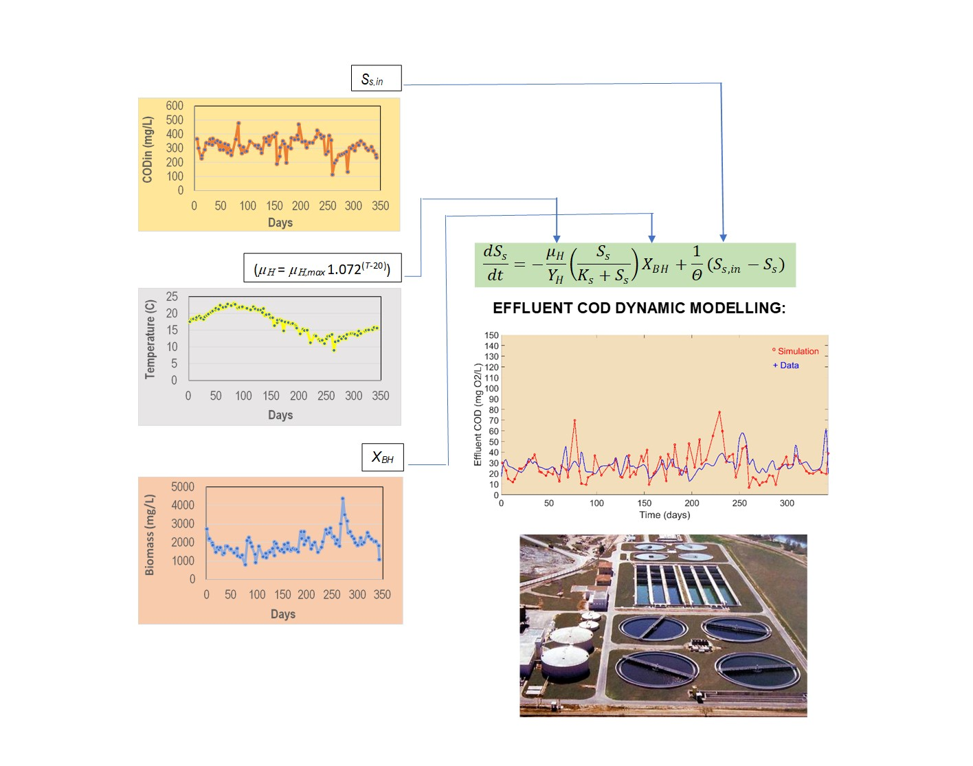
Equation (7) is the differential equation in which the simulation of effluent COD was obtained. Dynamic variables that affect the output COD value are biomass concentration (X_BH) and specific growth rate (μ_H); these are both influenced by temperature (μ_H = μ_H,max 1.072^(T−20)). S_s,in is also included as a dynamic variable because of daily fluctuations in the WWTP. Equation (7) was solved by MATLAB R2021b [6,22], adjusting the kinetic parameters Y_H and K_s, using the known range 0.40–0.75 for Y_H and using the medium value of effluent COD for K_s [23].

The protocol of simulation is separated into three steps for the approximation of the simulation line to the experimental data. In the first step (tuning on Y_H), the value of Y_H is obtained, in the range 0.5–0.7 for μ_H,max = 0.1 d⁻¹ as a fixed value. This value of the maximum specific growth rate is low for better visualisation of the dynamism of the simulation. In the second step (tuning on μ_H,max), the value of μ_H,max is selected maintaining the fixed value for Y_H obtained in the first step. In the third step (fine tuning on μ_H,max), the value of μ_H,max is carefully adjusted, comparing errors between the simulation and the experimental values.

2.5. Biological Treatment in WWTP

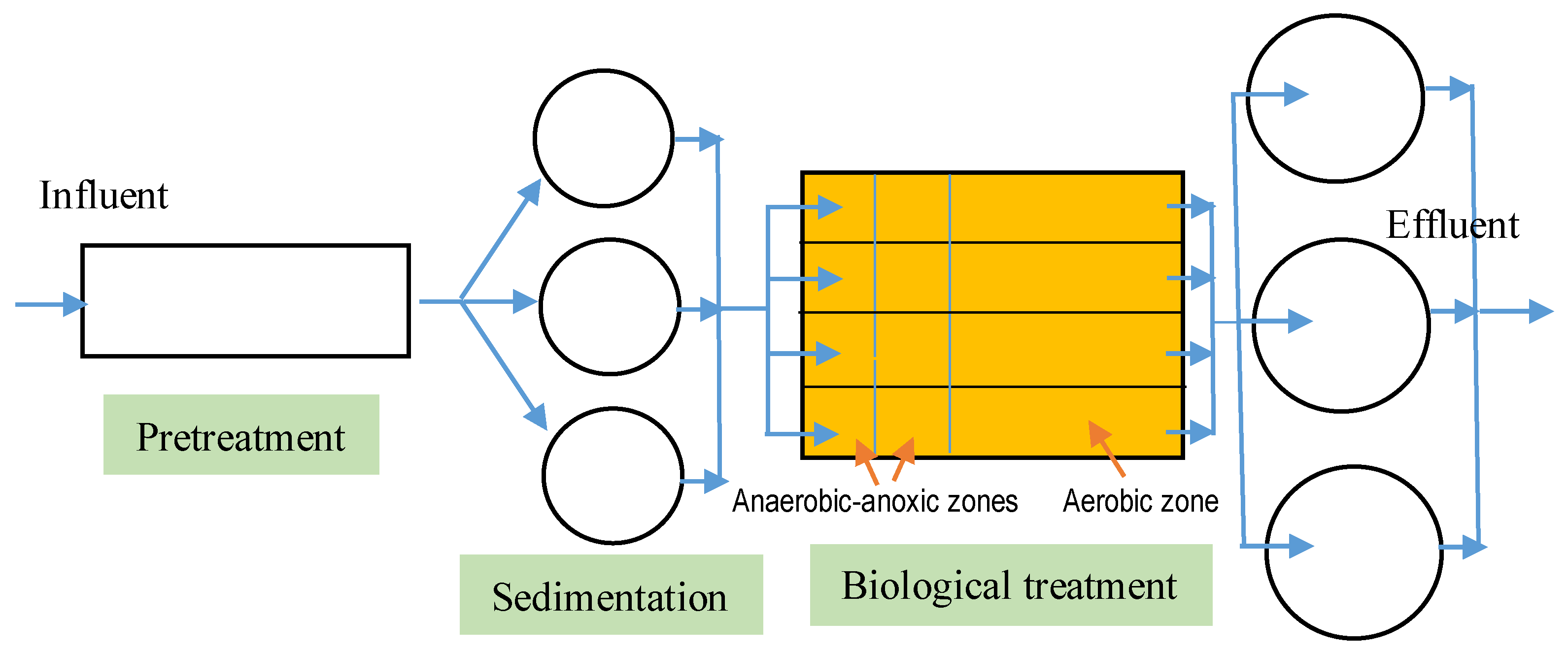
The wastewater treatment plant used in this study is a medium–high-sized plant, designed for 260,000 habitants of the city of Salamanca (Spain). The scheme of the treatment processes is described in Figure 2.

2.6. Analytical Methods

COD was analysed as total COD in influent and effluent of the biological treatment, following the standard method [24]. Biomass concentration in the biological reactor was determined as MLSS (mixed liquor suspended solids), which is the solid residue after evaporation at 103–105 °C in samples filtered by filters with a pore size of 0.45 μm [24]. The temperature was measured in the biological reactor by a thermocouple.

3. Results and Discussion

3.1. Dynamic Variables

The simulation of effluent COD in the biological treatment of a WWTP relies on the solution of Equation (7), in which X_BH, μ_H and S_s,in are the three dynamic variables included in the MATLAB programme, as time-dependent, discrete values (analysed values). These discrete values were obtained from

Table 3. Experimental values for biological treatment measured in the WWTP between May 2020 and April 2021 (343 days). Data were supplied by the staff of the WWTP.

Day	CODin	COD	Temp	Biomass
	(mg/L)	(mg/L)	(°C)	(mg/L)
1	----	23.7	17.6	2723
5	367	32.9	18.3	2160
7	302	27.3	18.5	2210
12	229	25.3	18.3	1967
14	250	24.1	18.9	1850
19	290	21.6	19.2	1477
21	338	21.0	18.7	1730
26	331	27.2	18.4	1623
29	365	34.1	19.0	1720
33	326	29.3	19.5	1367
35	369	31.1	19.8	1433
40	342	25.9	20.5	1790
42	354	25.6	20.8	1787
47	290	23.7	21.1	1610
49	342	23.9	21.6	1647
54	291	26.2	21.4	1470
56	331	23.7	22.5	1447
61	269	18.6	21.7	1677
63	324	24.3	21.8	1277
68	284	45.6	22.0	1210
70	251	22.4	22.8	1310
77	364	31.4	22.4	810
82	478	25.9	22.9	2103
84	321	40.6	22.8	2263
89	265	21.5	21.6	1993
91	308	21.5	21.8	1770
96	278	21.1	21.8	1357
98	280	19.3	22.1	917
105	350	26.7	21.6	1790
113	321	27.5	21.1	1227
118	303	29.9	22.1	1410
120	322	35.0	21.4	1177
125	296	17.8	21.1	1527
127	267	22.7	21.1	1480
132	373	37.0	21.0	1673
134	368	30.2	20.3	1300
135	347	26.7	21.5	2027
139	384	26.9	19.5	1945
141	326	25.0	19.7	1715
147	390	27.2	19.8	1560
149	382	28.3	18.8	1623
153	408	23.6	18.8	1485
155	189	15.4	16.5	1895
160	244	18.1	17.4	1650
162	306	20.2	18.1	1968
167	352	27.6	18.1	1553
169	332	33.2	17.8	1618
173	198	23.2	14.9	1675
175	311	25.8	17.5	1635
180	300	33.9	17.2	1608
182	372	25.9	17.4	1490
187	369	24.7	17.0	2590
189	361	17.7	17.0	2215
194	392	27.3	16.5	2590
195	365	24.1	16.1	1895
197	469	12.6	15.7	2105
203	347	18.6	14.0	2255
208	349	24.9	15.4	1665
210	306	23.5	14.9	1860
215	340	29.5	15.1	2008
222	341	26.9	11.4	1475
229	379	37.3	13.5	1748
232	427	38.9	13.4	2045
236	396	32.1	12.2	2690
239	372	30.5	11.9	2483
243	384	30.7	12.1	2525
246	259	23.5	11.1	2778
250	277	53.2	12.5	2283
253	390	58.1	13.2	2325
257	358	49.5	13.3	1948
260	114	28.1	13.8	2133
264	196	33.3	9.1	1808
267	215	24.0	11.6	3013
271	251	20.3	11.8	4375
274	253	24.8	13.0	3510
278	259	20.7	12.5	3165
281	264	27.4	13.1	2533
285	275	32.1	12.6	2575
288	134	23.6	13.8	2343
292	304	24.1	14.0	2205
295	300	26.8	14.1	1983
299	319	28.8	14.1	1838
301	284	24.3	13.9	1855
306	334	26.9	13.5	2260
309	323	47.6	14.8	1913
313	352	28.6	14.1	2008
320	329	30.8	14.7	2530
323	301	27.1	15.1	2340
327	287	22.7	15.1	2190
334	310	24.5	15.2	2050
336	283	27.4	15.9	2060
341	254	62.1	15.8	1830
343	235	19.9	15.7	1090

.

3.2. Tuning on Y_H

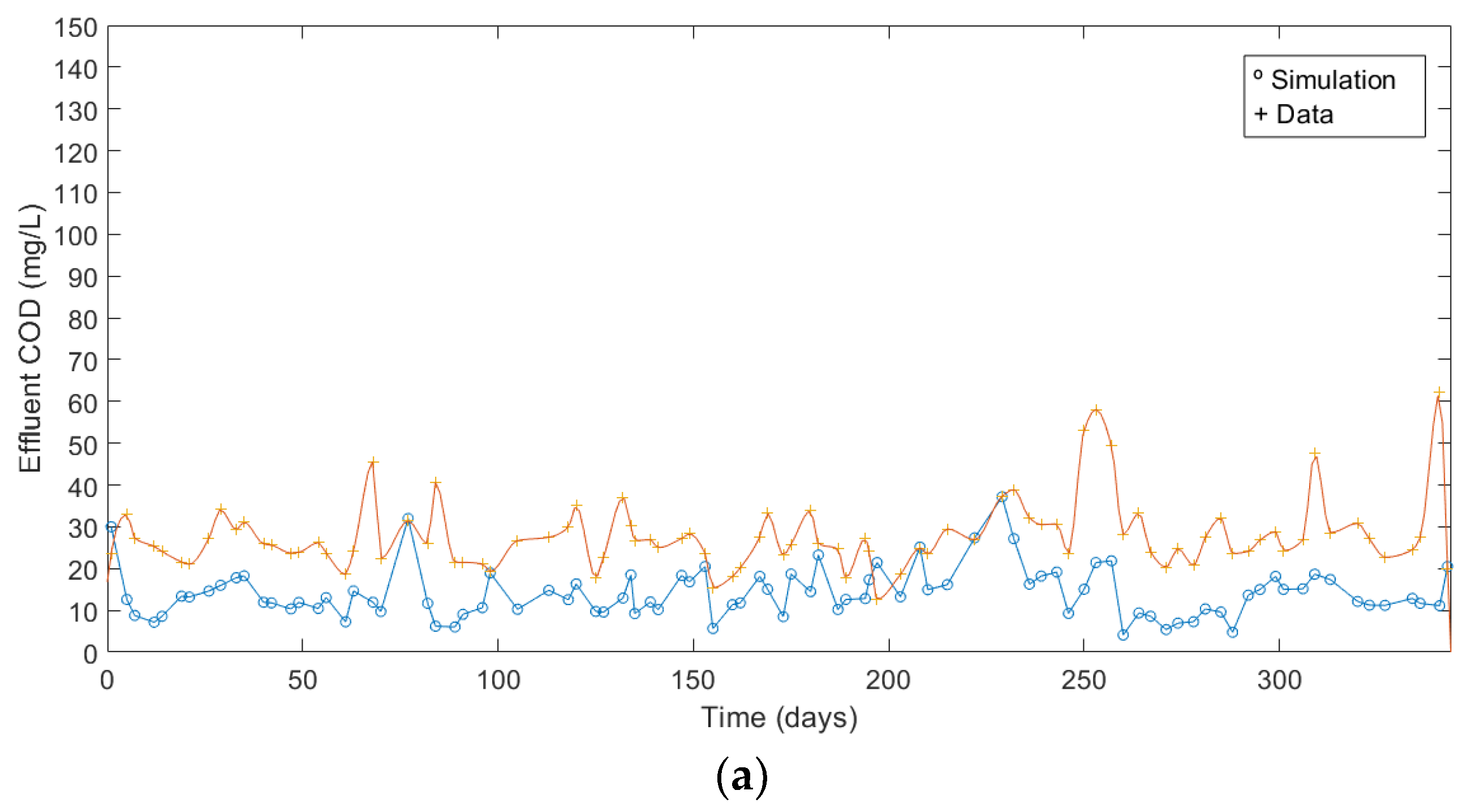
Tuning is the operation in which the simulation is adjusted to make it coincide with the experimental data. The first time that the dynamic model response is checked, the behaviour of Y_H should be assayed. The initial value of μ_H,max normally marks the baseline of the simulation, and, in this first approximation, it was decided that μ_H,max would be low for better visualisation of the mathematical response to the output of COD and the dynamic variables, because the dynamism was expected to be reduced, increasing the μ_H,max value. The value selected was μ_H,max = 0.1 d⁻¹ (Figure 3), a low value compared with the ranges for domestic wastewater in the literature: 0.45–1.0 d⁻¹ [16], 0.6–13.2 d⁻¹ [23], and 3.0–13.2 d⁻¹ for the original ASM1 [1] were proposed. For tuning on Y_H, K_s = 27.7 mg/L (average value of effluent COD) and Θ = 14.8 h (biological process of WWTP in Figure 2).

The main conclusion (Figure 3) in the prediction of the output S_s value in the WWTP is that the higher the fraction of substrate incorporated into the biomass, the higher the concentration of remaining organic matter after the biological treatment (Y_H = 0.7 elevates the simulation line).

The elevation of the simulation line when the Y_H value was incremented can be explained by the fact that the formation of the biomass is a slow process (synthesis reaction), compared to the transformation of organic matter (oxidation reaction).

Mathematically, increasing the Y_H value in Equation (7) makes the derivative of S_s less negative, because the negative term normally has a higher value in the equation, leading to a smaller decrease from the initial value (output substrate value rises).

The value assumed for Y_H in the literature is normally 0.6 [5,11,12], and this is the fixed value used in subsequent tuning assays.

3.3. Tuning on μ_H,max

Specific growth rates are strongly affected by temperature in biological processes. The mathematical expression of this influence is μ_H = μ_H,max 1.072^(T−20), and modification of the μ_H,max value will generate an inverse response on S_s. Increments in μ_H,max will decrease the effluent organic matter concentration (S_s), because the substrate will be degraded to a greater extent.

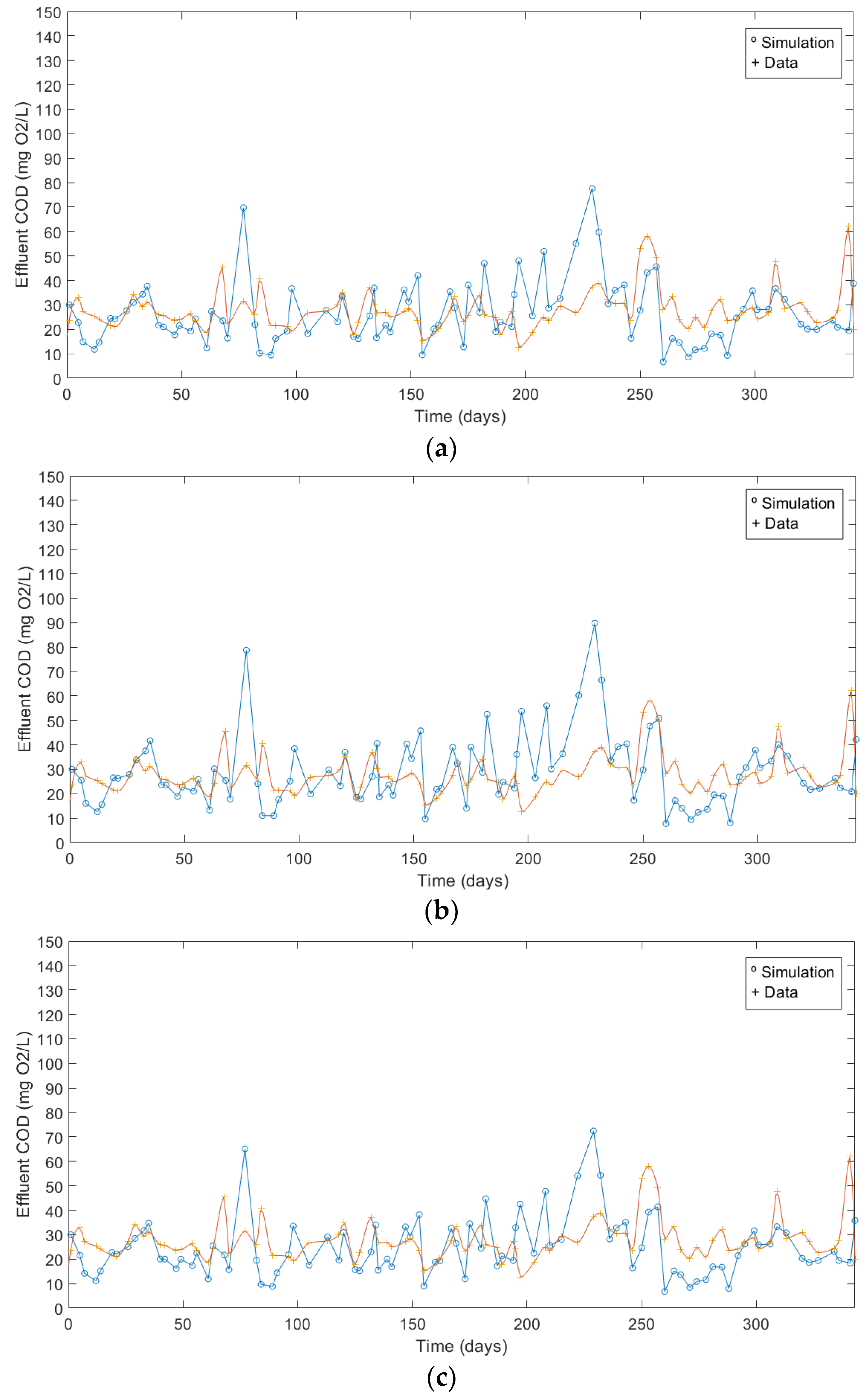
Figure 4 shows two situations, in which the simulation results in an underestimation (a), where the simulation line predicts lower values of organic matter concentration (μ_H,max = 0.6 d⁻¹), and in an overestimation (b), with the simulation line over the line of experimental data (μ_H,max = 0.3 d⁻¹). The simulation will be coincident for a value of μ_H,max in between those values.

On the other hand, comparing the graphs in Figure 4, increments in the μ_H,max value lowered the dynamism in the dynamic model simulation (Figure 4a,c), and fluctuations in the output value were higher when μ_H,max was lower (Figure 4b). Increasing the μ_H,max value tempers dynamism because the simulation reduced the fluctuations of the output parameter (more visible for a higher reduction in substrate), which means higher actuation of the dynamic model in Equation (7) [25,26].

3.4. Fine Tuning on μ_H,max

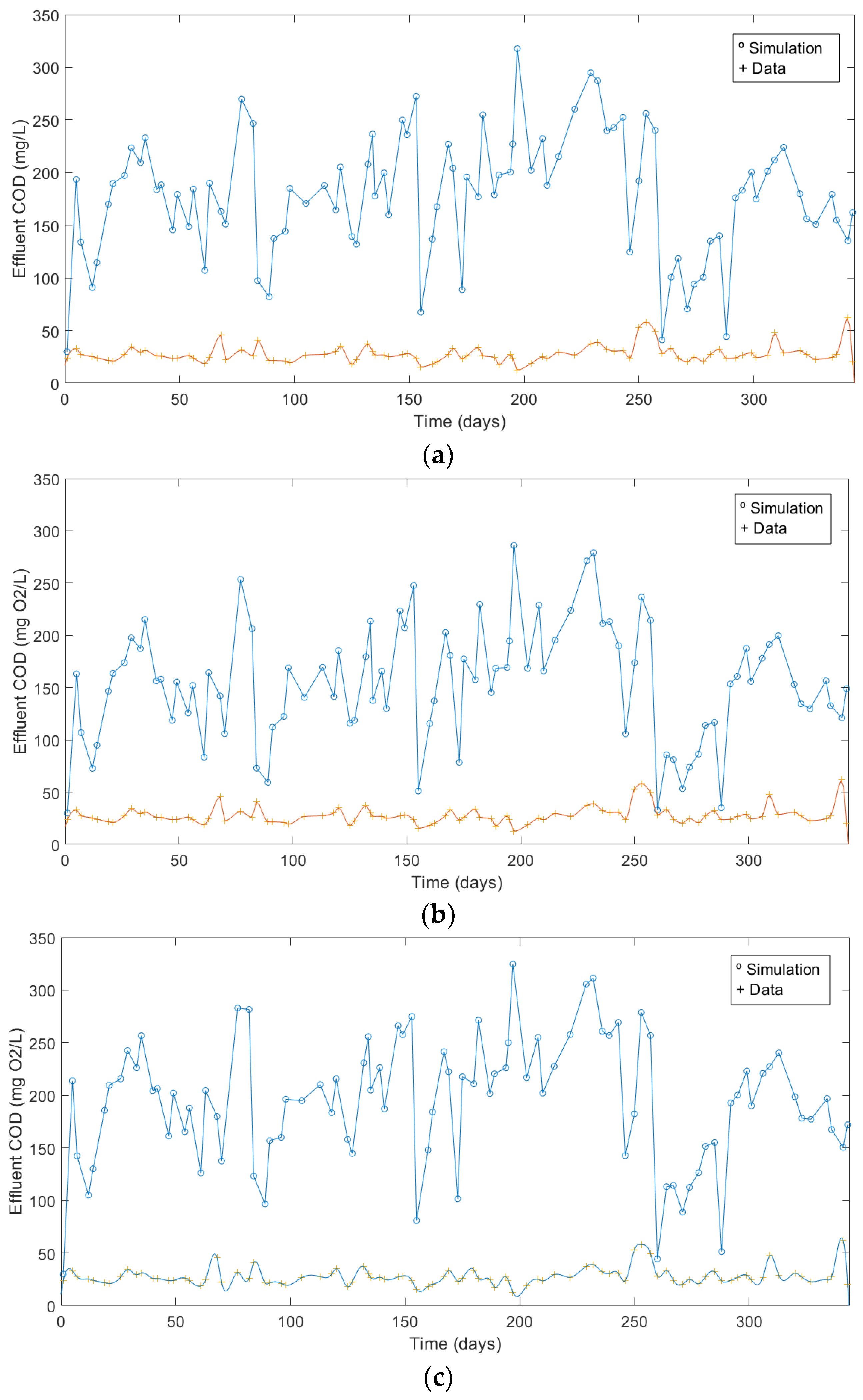
When the simulation is approximated to the analysed data (Figure 4c), quantification of fitting (fine tuning) in the dynamic model, visualised in Figure 5, has to be performed. In Table S1 (Supplementary Material), the average error between the simulated and analysed data is presented, after the COD and simulated values in the table. In this case, the fine tuning in Figure 5 was solved for μ_H,max values close to 0.40 d⁻¹ (0.38 and 0.42), with Y_H = 0.60 as a fixed value. The error is calculated by considering the analysed value as the true value, as follows:

$$Error=\frac{\left(simulated value-analysed value\right)}{analysed value}\times 100$$

The average errors show an overestimation for μ_H,max = 0.38 d⁻¹ (error = 8.1%) and an underestimation for μ_H,max = 0.42 d⁻¹ (error = −7.7%). The minimum error between the simulated and analysed values (COD (mg/L)) was obtained for μ_H,max = 0.40 d⁻¹ (error = −0.5%), which was the value selected for the maximum specific growth rate of the community of microorganisms in the studied biological treatment of the WWTP. This value of μ_H,max is very close to the range 0.45–1.0 d⁻¹ proposed by other authors [16,27]; although, in other articles, the proposed value is higher [28].

In Table S1 (Supplementary Material), high values of individual relative errors can be observed (as visualised in Figure 5). This is a normal result in dynamic simulations of biological treatments [15], in which the consequences of a “live” system are often observed. The main reasons for overestimation and underestimation of the dynamic mathematical model are especially related to the activity of biomass (active and inert fractions), attenuation and inertial effect of the bacterial community on fluctuations in temperature, the flow rate, and the substrate concentration [29,30]. A dynamic mathematical model does not reproduce this behaviour of the bacterial community, no theoretical model is able to do this, but its utility, especially for the prediction of the response to perturbations and the oscillatory behaviour of the output parameter, is evident [31].

4. Conclusions

The ASM1 is the basis for the mathematical modelling of organic matter reduction in aerobic biological wastewater treatment systems. Although the original model was published more than 30 years ago, the configuration and flexibility of this model make it almost universal in the explanation of biological treatment processes.

Understanding how it was formulated and how it works is of great value for the mathematical modelling of real systems, and for new proposals in the modelling of special systems. One of the most important steps in ASM1 use is the selection of the processes involved after the components are selected. Adjustment and simplification of the dynamic model are crucial for the correct application of this useful model.

When applying ASM1 dynamic modelling for the prediction of a WWTP, tuning on Y_H and μ_H,max has to be elaborated. In the case of the WWTP of Salamanca (Spain, 260,000 habitants), Ks is fixed as the average value of effluent COD (Ks = 27.7 mg/L), and Θ is in accordance with the reactor volume and the influent flow rate (Θ = 14.8 h). Assuming a short range of Y_H values (0.40–0.75) in the protocol of simulation proposed in this article, in which the approximation of the simulation line to the experimental data is performed in three steps, tuning on Y_H, conducts to Y_H = 0.60, and tuning on μ_H,max, after the approximation of the baseline and dynamism, comparative errors between the simulated and analysed data mark the correct value (fine tuning, μ_H,max = 0.40 d⁻¹).

Individual errors are high in the dynamic modelling of biological treatments; a live system reproduced by a mathematical model will inevitably lead to this result, but utility in the prediction of the oscillatory behaviour of the output parameter value, especially when environmental perturbations occur, is essential.

References

- Henze, M.; Grady, C.P.L.; Gujer, W.; Marais, G.V.R.; Matsuo, T. A general model for single-sludge wastewater treatment systems. Water Res. 1987, 21, 505–515. [Google Scholar] [CrossRef] [Green Version]
- Gujer, W.; Henze, M.; Mino, T.; Matsuo, T.; Wentzel, M.C.; Marais, G.V.R. The activated sludge model no. 2: Biological phosphorus removal. Water Sci. Technol. 1995, 31, 1–11. [Google Scholar] [CrossRef]
- Gujer, W.; Henze, M.; Mino, T.; van Loosdrecht, M. Activated sludge model no.3. Water Sci. Technol. 1999, 39, 183–193. [Google Scholar] [CrossRef]
- Henze, M.; Gujer, W.; Mino, T.; Matsuo, T.; Wentzel, M.C.; Marais, G.V.R.; van Loosdrecht, M. Activated sludge model no. 2d. ASM2D. Water Sci. Technol. 1999, 39, 165–182. [Google Scholar] [CrossRef]
- Henze, M.; Gujer, W.; Mino, T.; van Loosdrecht, M. Activated Sludge Models ASM1, ASM2, ASM2d and ASM3; IWA Scientific and Technical Report No. 9; IWA Publishing: London, UK, 2000. [Google Scholar]
- Gernaey, K.V.; van Loosdrecht, M.; Henze, M.; Lind, M.; Jorgensen, S.B. Activated sludge wastewater treatment plant modelling and simulation: State of the art. Environ. Model. Softw. 2004, 19, 763–783. [Google Scholar] [CrossRef]
- Iacopozzi, I.; Innocenti, V.; Marsili-Libelli, S.; Giusti, E. A modified activated sludge model no. 3 (ASM3) with two-step nitrification-denitrification. Environ. Model. Softw. 2007, 22, 847–861. [Google Scholar] [CrossRef]
- Brun, R.; Kühni, M.; Siegrist, H.; Gujer, W.; Reichert, P. Practical identifiability of ASM2d parameters-systematic selection and tuning of parameter subsets. Water Res. 2002, 36, 4113–4127. [Google Scholar] [CrossRef]
- Reijken, C.; Giorgi, S.; Hurkmans, C.; Pérez, J.; van Loosdrecht, M. Incorporating the influent cellulose fraction in activated sludge modelling. Water Res. 2018, 144, 104–111. [Google Scholar] [CrossRef]
- Hu, H.; Liao, K.; Xie, W.; Wang, J.; Wu, B.; Ren, H. Modeling the formation of microorganism-derived dissolved organic nitrogen (mDON) in the activated sludge system. Water Res. 2020, 174, 115604. [Google Scholar] [CrossRef]
- Wu, X.; Yang, Y.; Wu, G.; Mao, J.; Zhou, T. Simulation and optimization of a coking wastewater biological treatment process by activated sludge models (ASM). Waste Manag. 2016, 165, 235–242. [Google Scholar] [CrossRef]
- Zhao, J.; Huang, J.; Guan, M.; Zhao, Y.; Chen, G.; Tian, X. Mathematical simulating the process of aerobic granular sludge treating high carbon and nitrogen concentration wastewater. Chem. Eng. J. 2016, 306, 676–684. [Google Scholar] [CrossRef]
- Baeten, J.E.; van Loosdrecht, M.; Volcke, E.I.P. Modelling aerobic granular sludge reactors through apparent halfsaturation coefficients. Water Res. 2018, 146, 134–145. [Google Scholar] [CrossRef] [PubMed]
- Du, X.; Ma, Y.; Wei, X.; Jegatheesan, V. Optimal Parameter Estimation in Activated Sludge Process Based Wastewater Treatment Practice. Water 2020, 12, 2604. [Google Scholar] [CrossRef]
- Spérandio, M.; Espinosa, M.C. Modelling an aerobic submerged membrane bioreactor with ASM models on a large range of sludge retention time. Desalination 2008, 231, 82–90. [Google Scholar] [CrossRef]
- Fenu, A.; Guglielmi, G.; Jimenez, J.; Spérandio, M.; Saroj, D.; Lesjean, B.; Brepols, C.; Thoeye, C.; Nopens, I. Activated sludge model (ASM) based modelling of membrane bioreactor (MBR) processes: A critical review with special regard to MBR specificities. Water Res. 2010, 44, 4272–4294. [Google Scholar] [CrossRef]
- Wágner, D.S.; Valverde-Pérez, B.; Sæbø, M.; Bregua de la Sotilla, M.; van Wagenen, J.; Smets, B.F.; Plósz, B.G. Towards a consensus-based biokinetic model for green microalgae-The ASM-A. Water Res. 2016, 103, 485–499. [Google Scholar] [CrossRef] [Green Version]
- Santos, J.M.M.; Rieger, L.; Lanham, A.B.; Carvalheira, M.; Reis, M.A.M.; Oehmen, A. A novel metabolic-ASM model for full-scale biological nutrient removal systems. Water Res. 2020, 171, 115373. [Google Scholar] [CrossRef]
- Acevedo, V.; Kaiser, T.; Babist, R.; Fundneider, T.; Lackner, S. A multi-component model for granular activated carbon filters combining biofilm and adsorption kinetics. Water Res. 2021, 197, 117079. [Google Scholar] [CrossRef]
- Lahdhiri, A.; Lesage, G.; Hannachi, A.; Heran, M. Steady-State Methodology for Activated Sludge Model 1 (ASM1) State Variable Calculation in MBR. Water 2020, 12, 3220. [Google Scholar] [CrossRef]
- Orhon, D.; Yucel, A.B.; Insel, G.; Solmaz, B.; Mermutlu, R.; Sözen, S. Appraisal of Super-Fast Membrane Bioreactors by MASM—A New Activated Sludge Model for Membrane Filtration. Water 2021, 13, 1963. [Google Scholar] [CrossRef]
- Smets, I.Y.; Haegebaert, J.V.; Carrette, R.; van Impe, J.F. Linearization of the activated sludge model ASM1 for fast and reliable predictions. Water Res. 2003, 37, 1831–1851. [Google Scholar] [CrossRef]
- Sharifi, S.; Murthy, S.; Takács, I.; Massoudieh, A. Probabilistic parameter estimation of activated sludge processes using Markov Chain Monte Carlo. Water Res. 2014, 50, 254–266. [Google Scholar] [CrossRef] [PubMed]
- APHA; AWWA; WEF. Standard Methods for the Examination of Water and Wastewater, 23rd ed.; American Public Health Association: Washington, DC, USA, 2017. [Google Scholar]
- Meijer, S.C.F.; van Loosdrecht, M.; Heijnen, J.J. Modelling the start-up of a full-scale biological phosphorous and nitrogen removing WWTP. Water Res. 2002, 36, 4667–4682. [Google Scholar] [CrossRef]
- Plattes, M.; Henry, E.; Schosseler, P.M.; Weidenhaupt, A. Modelling and dynamic simulation of a moving bed bioreactor for the treatment of municipal wastewater. Biochem. Eng. J. 2006, 32, 61–68. [Google Scholar] [CrossRef]
- Spérandio, M.; Massé, A.; Espinosa, M.C.; Cabassud, C. Characterization of sludge structure and activity in submerged membrane bioreactor. Water Sci. Technol. 2005, 52, 401–408. [Google Scholar] [CrossRef]
- Wang, C.; Zeng, Y.; Lou, J.; Wu, P. Dynamic simulation of a WWTP operated at low dissolved oxygen condition by integrating activated sludge model and floc model. Biochem. Eng. J. 2007, 33, 217–227. [Google Scholar] [CrossRef]
- Costa, C.; Rodríguez, J.; Márquez, M.C. A simplified dynamic model for the activated sludge process with high strength wastewaters. Environ. Model. Assess. 2009, 14, 739–747. [Google Scholar] [CrossRef]
- Tamrat, M.; Costa, C.; Márquez, M.C. Biological treatment of leachate from solid wastes: Kinetic study and simulation. Biochem. Eng. J. 2012, 66, 46–51. [Google Scholar] [CrossRef]
- Costa, C.; Domínguez, J.; Autrán, B.; Márquez, M.C. Dynamic modeling of biological treatment of leachates from solid wastes. Environ. Model. Assess. 2018, 23, 165–173. [Google Scholar] [CrossRef]
Figure 1.
CSTR scheme for the ASM1. ξ is the vector of reactor and effluent concentration, ξin is the vector of influent concentration, Q is the influent flow rate, and V is the reactor volume.
Figure 2.
Scheme of the WWTP. Average influent flow rate was 60,466 m3/d during the measuring time. Total biological reactor volume (orange colour) was 37,240 m3, 4 chambers of 9310 m3 (Θ = 14.8 h), and oxygen concentration was maintained in 1.5 ± 0.3 mg/L.
Figure 3.
Tuning on YH for μH,max = 0.1 d−1. (a) YH = 0.6, (b) YH = 0.5 and (c) YH = 0.7. Blue upper line is simulation data and coloured lower line is the evolution of real values (analysed data) after biological treatment in the WWTP (Table 3, COD (mg/L)).
Figure 4.
Tuning on μH,max for YH = 0.6. (a) μH,max = 0.6 d−1, (b) μH,max = 0.3 d−1 and (c) μH,max = 0.5 d−1. Simulation is the blue line and analysed data is the orange line.
Figure 5.
Fine tuning on μH for YH = 0.60. (a) μH,max = 0.40 d−1, (b) μH,max = 0.38 d−1 and (c) μH,max = 0.42 d−1.