
A Simple Approach to Account for Stage–Discharge Uncertainty in Hydrological Modelling


1
Laboratorio de Ecología Acuática (LEA), Facultad de Ciencias Químicas, Universidad de Cuenca, Av. 12 de Abril S/N y Av. Loja, Cuenca 010203, Ecuador
2
Departamento de Ingeniería Civil, Facultad de Ingeniería, Universidad de Cuenca, Av. 12 de Abril S/N y Av. Loja, Cuenca 010203, Ecuador
*
Author to whom correspondence should be addressed.
Water 2022, 14(7), 1045; https://doi.org/10.3390/w14071045
Submission received: 14 January 2022
/
Revised: 22 February 2022
/
Accepted: 24 February 2022
/
Published: 26 March 2022
(This article belongs to the Topic Hydrological Modeling and Engineering: Managing Risk and Uncertainties)
Abstract
:The effect of stage–discharge (H-Q) data uncertainty on the predictions of a MIKE SHE-based distributed model was assessed by conditioning the analysis of model predictions at the outlet of a medium-size catchment and two internal gauging stations. The hydrological modelling was carried out through a combined deterministic–stochastic protocol based on Monte Carlo simulations. The approach considered to account for discharge uncertainty was statistically rather simple and based on (i) estimating the H-Q data uncertainty using prediction bands associated with rating curves; (ii) redefining the traditional concept of residuals to characterise model performance under H-Q data uncertainty conditions; and (iii) calculating a global model performance measure for all gauging stations in the framework of a multi-site (MS) test. The study revealed significant discharge data uncertainties on the order of 3 m3 s−1 for the outlet station and 1.1 m3 s−1 for the internal stations. In general, the consideration of the H-Q data uncertainty and the application of the MS-test resulted in remarkably better parameterisations of the model capable of simulating a particular peak event that otherwise was overestimated. The proposed model evaluation approach under discharge uncertainty is applicable to modelling conditions differing from the ones used in this study, as long as data uncertainty measures are available.
1. Introduction
River discharge measurements are rather important for water resources management [1,2,3,4,5,6] and modelling [7,8,9]. Despite recent technical progress in direct discharge measurement, both with regards to on-site [10,11] and remotely sensed [12,13] estimates, the continuous collection of river discharge information still relies on deriving discharges from records of water stages. Such approaches are easier and less expensive to acquire than others and are based on establishing a stage–discharge (rating) curve in a given control cross-section [3,6,14,15,16,17].
Practitioners (and even researchers) commonly rely on rating curves without, however, considering that there might be considerable uncertainty in their development [12,18,19] arising from errors incurred while interpolating or extrapolating the rating curve or errors owing to seasonal (or even man-induced) changes in the control river section [6]. The latter is particularly true for high flows because they are difficult to measure owing to practical constraints [2,7], although low flows uncertainty may also be significant [16]. Moreover, under certain circumstances, the stage–discharge relationship might not be unique, which is normally manifested through multiple hysteresis loops in the measures [6,8,15,18,20].
As such, data uncertainty identification [17,21,22,23,24] and the assessment of its effects on hydrological–hydraulic modelling [25,26,27,28] is needed. Nevertheless, national and/or regional meteorological services rarely report data on the rating curve being used or the stage being considered. Furthermore, these agencies typically do not assess the fundamental reliability of such observed data and/or the resulting rating curve [29]. Although significant research has been carried out on statistically complex methods for quantifying uncertainty in discharge data [2,16,17,20,21,22,24,26,29,30,31,32,33,34], there has not been abundant research on user friendly (i.e., simpler) methods for the same purpose. Together, this means there are few reported applications of the more complex methods in practice (i.e., applications made in non-research modelling studies), despite the availability of especially dedicated software (i.e., [26]).
Water resources modelling, whether using probabilistic models and/or machine learning techniques that highly rely on perfectness of observed data, is of course being carried out in many practical settings without explicit consideration of discharge data uncertainties (i.e., [35,36]). Still, significant research on the implications of data uncertainty, including stage–discharge uncertainty, on water resources modelling has come forward more recently. For example, Aronica, et al. [37]; Pappenberger, et al. [38]; Huard and Mailhot [39]; Bales and Wagner [25]; Liu, et al. [40]; Krueger, et al. [41]; McMillan, et al. [42], Domeneghetti, et al. [43], Bermudez, et al. [44], Ocio, Le Vine, Westerberg, Pappenberger, and Buytaert [2]; Westerberg, Sikorska-Senoner, Viviroli, Vis and Seibert [33]; and Kastali, et al. [45] collectively constitute some of the recent studies dealing with the effects of the stage–discharge uncertainty on water resources modelling. However, nearly all these studies involve the use of complex statistical methods aiming at defining explicit probability density functions (PDF) of true discharge, which makes difficult to use them in practice. Furthermore, most of the aforementioned studies have focused on single-site discharge modelling (except under well controlled experimental conditions [41]), which is a limitation when evaluating distributed model predictions in real-world applications.
In this context, the research questions that motivated the current study are as follows. (i) Is there a simple yet accurate way for estimating the uncertainty associated with the stage–discharge data under non-research conditions? (ii) Is it feasible to adapt commonly used model evaluation approaches that explicitly consider stage–discharge uncertainties without the use of a complex statistical framework? (iii) Is it possible to expand such model evaluation approaches by considering the prediction of discharges at different sites within the modelling domain (multi-site (MS) evaluation test)? (iv) Is it feasible to improve model identification (or model rejection) with regards to the application of conventional model evaluation approaches that do not take into account explicitly stage–discharge uncertainties?
Correspondingly, the objectives of this study focused on: (i) adapting a conventional model evaluation protocol by considering simple approaches to explicitly account for stage–discharge uncertainties over multi-site discharge simulation; and (ii) applying the suggested model evaluation approaches to a distributed modelling of the study catchment. The methodological approach tested included (a) estimating stage–discharge (H-Q) data uncertainty using prediction bands associated with the rating curves; (b) redefining the traditional concept of residuals to characterise model performance under H-Q data uncertainty conditions using likelihood measures based on residuals; and (c) calculating a global model performance measure for all the gauging stations in the framework of a MS test.
While the main aim of this paper was to work out a simple way of estimating stage–discharge uncertainty and its implication in hydrological modelling, the intention of the authors is far from suggesting to the reader that the use of more complex statistical approaches for the same purpose should not be considered. On the contrary, given their elaborated statistical background, these more complex statistical approaches are likely to be more accurate than the simpler approaches suggested in this paper. Nevertheless, facing the possibility of not applying any stage–discharge uncertainty assessment in non-research hydrological modelling, the approaches herein developed may be an acceptable alternative for practitioners (and even researchers) depending on the modelling objectives at hand.
2. Materials and Methods
2.1. The Study Site
The Gete catchment (Figure 1) has a surface area of about 586 km2. It is formed by the Kleine Gete (260 km2) and the Grote Gete (326 km2) sub-catchments. Elevation of the study area ranges from approximately 27 m in the north to 174 m in the south. Land use is mainly agricultural, with a predominance of pasture and cultivated fields while some local forested areas are also present. The catchment area is covered by nine soil units comprising loamy (predominant), sand-loamy, and clay soils, as well as soils with stony mixtures. Moderate humid conditions are observed in the catchment. The reader is referred for instance to [46] for additional details about the characteristics of the study site.
2.2. Hydrometeorological Data
Different hydrometeorological records were available for the current modelling, including discharge (Q) data derived from stage (H) observations on the basis of rating curves [47] for the Gete and Kleine Gete stations, both located at Budingen, and for the Grote Gete station, located at Hoegaarden (Figure 1). Furthermore, the set of original measures that were used to define the H-Q rating curves of the gauging stations Gete and Kleine Gete were also available for this study. Observations were collected at the following intervals: (24 January 1983–31 May 1995) for the Gete station and (4 June 1985–31 May 1995) for the Kleine Gete station. A total of 49 stage–discharge observations were available for the Gete station and 38 observations for the Kleine Gete.
The Flemish Administration for Environment, Nature, Land, and Water (AMINAL), Division WATER, was responsible for the collection of discharge related data at the Gete and Kleine Gete gauging stations. The Grote Gete station, on the other hand, was managed by a different water authority, namely the Service for Hydrological Research (DIHO) of the Ministry of Public Works. Information on the discharge measures to define the Grote Gete rating curve was not available for this study.
In this context, Figure 2 shows the distribution of the sampled points for the Gete and Kleine Gete gauging stations. Henceforth, for either station, although there is a higher concentration of low flow observations, there is also an acceptable number of mid-flow and high flow observations, which is not typical. This rather uniform distribution of sampled points (i.e., gaugings) throughout most of the range of discharges is likely to produce uncertainty bounds that are also rather uniform without a significant accentuation for larger flows. Furthermore, no data loops or hysteresis were perceived for the set of observations available, which supports the use of relatively simple expressions of the relationship between H and Q at these gauging stations.
2.3. The Hydrologic Code
The MIKE SHE code [49] was used for the integral hydrological modelling of the study site. It is a deterministic-distributed code that is used and described in a wide range of applications [9,50,51,52]. It is capable of simulating interception (Rutter model), actual evapotranspiration (ETact; Kristensen and Jensen model), overland flow (two-dimensional, kinematic wave), channel flow (one dimensional, diffusive wave), flow in the unsaturated zone (one dimensional, Richards’ equation), flow in the saturated zone (two- or three-dimensional, Boussinesq equation), and exchange between aquifers and rivers. When using MIKE SHE in a catchment-scale framework, it is implicitly assumed that smaller scale equations (e.g., those that are embedded in the mathematical structure of MIKE SHE) are also valid on a larger (catchment) scale through the use of effective model parameters that implicitly perform an upscaling operation from field conditions. The MIKE SHE hydrological model uses a square-grid finite difference simulation scheme.
2.4. Estimating the Uncertainty Attached to Stage–Discharge Data
Here, we present a simple approach to estimate the uncertainty of discharge data available for the hydrological modelling considered. Since the components of the general modelling evaluation approach are independent of the uncertainty estimate approach, the reader is free to apply any other relevant procedure for deriving discharge uncertainty estimates (i.e., [2,16,17,20,21,22,24,26,29,30,31,32,34]) or use already existing uncertainty estimates. Nevertheless, owing to its simplicity compared to much more complex stochastic methods reported in literature, the current uncertainty estimate approach is likely to be a suitable approach for most practitioners and researchers.
Originally, Q was derived from H observations based on rating curves, which were obtained through regression analysis [47] by considering the following general polynomial expression:
where Q [L3 T−1] and (H − H0) [L] are regression variables, ai is the ith regression coefficient [L3−ei T−1], ei is the ith regression exponent [––], i is an integer index [––], and l is an integer value defining the polynomial order [––]. H0 is a lower stage benchmark [L], above which the rating curve is acceptably described by Equation (1). Q, (H − H0), and ai are positive real numbers. When ei is a positive integer number, then Equation (1) is the expression for the polynomial regression of order l. When ei adopts any positive real value, a1 ≠ 0.0 and ai = 0.0 for i ≠ 1, then Equation (1) is the expression for the power regression. Q was considered as the dependent variable, whilst (H − H0) was treated as the independent variable. Equation (1) was used in the current study by considering observational data originally utilised to derive the rating curve [47].
Since the aim of defining the rating curve is to use it for predicting Q for future H values, its prediction interval for a 90% confidence level was used herein as an estimate of the data uncertainty attached to the H-Q relationship (Figure 2). The prediction interval (always wider than the confidence interval) represents the range within which the true discharge value can reasonably be expected to be found for a particular future value of H. The choice of the form of the regression method is ultimately the responsibility of the modeller and depends on the problem being considered. However, the prediction interval of the chose regression method could be used to estimate discharge data uncertainties as is done in here.
The above approach was applied to the Gete and Kleine Gete stations where appropriate information was available. The approach was not applied in the case of the Grote Gete station since adequate information on its rating curve definition was not available. Consequently, prediction (i.e., uncertainty) bounds could not be estimated in a similar way for this station. Instead, a constant data uncertainty interval was assumed using the average prediction interval width obtained for the Kleine Gete station. This interval was slightly increased (subjectively, by 10%) to reflect broader uncertainty associated with this case.
Data regression and the estimation of the prediction intervals were carried out using different software to cross check results and prepare figures. These included R®, Statistica®, StatGraphics®, and MS-Excel®. Furthermore, Practical Extraction and Report Language (PERL) subroutines were prepared for both processing information prior to the statistical analysis as well as for processing the results of the regression analyses and defining the time series of prediction bounds to be used in the hydrological modelling. Moreover, GNUPLOT® [53] was used in conjunction with PERL for automatic plotting purposes to display results.
2.5. Initial Parameterisation of the Hydrological Model
In the following, an overview of the study site model is presented. For additional details, the reader may consult Vázquez, Feyen, Feyen, and Refsgaard [46]; Vázquez et al. [54]; or Vázquez and Hampel [52].
Spatial variation of precipitation in the study site was captured using Thiessen polygons defined for seven rainfall stations. Potential evapotranspiration (ETp) was estimated by combining crop coefficients (Kc) and the crop reference (i.e., grass) potential evapotranspiration (ET0), which was in turn estimated by means of the modified Penman FAO-24 method [48]. Literature [48,49] values were adopted and assumed being constant for the parameters of the actual evapotranspiration (ETact) module of MIKE SHE [49].
A Bilinear interpolation method [49], available in the MIKE SHE interface, was used to define the digital elevation model (DEM) of the study catchment using available point elevation data. The MIKE SHE river model was based on interpolation and extrapolation of a few measured stream profiles. River and overland flow roughness was represented using Strickler coefficients adopted from literature [55]. Average values for river reaches were in the order of 20 m1/3 s−1 (i.e., about Manning’s n = 0.05 s m−1/3), which is a typical value for winding natural streams and channels with weeds and pools. For overland flow, Strickler values were defined in correspondence with vegetation cover and land use, ranging between 2 m1/3 s−1 (n = 0.5 s m−1/3, light underbrush) and 10 m1/3 s−1 (n = 0.1 s m−1/3, natural range) with most simulation cells having a value of 6 m1/3 s−1 (about n = 0.17 s m−1/3, dense grass/crops).
Land use spatial and temporal variation was explicitly considered in the model. Literature-based values [48] were used for root depth and leaf area index. Accurate information was available for delineating the spatial extent of the 9 soil units included in the study catchment and for assessing the hydro-physical characteristics of each unit. Thus, soil parameters were not included in the calibration analysis to avoid potential complications due to over-parameterisation.
Nine geological units form the lithostratigraphy of the study catchment [46]. Only two of them (Quaternarian, Kw, and Landeniaan, Ln) are in direct contact with most of the river network. Aquifers were given no-flow boundary conditions coincident with the topographical divide since no suitable measures were available to assess the real groundwater divide.
The study site was subdivided in grids with a resolution of 600 × 600 m² [46]. This is a coarse discretisation for the purpose of describing accurately hillslope dynamics; however, the number of grid elements used in this study (ngr = 1629) is larger than what has been used in some previous similar applications of MIKE SHE (i.e., [50]), where the number of modelled geological layers (6, after a simplification of the observed vertical succession of units [46]) created a complex arrangement of calculation grids leading to a large computational time for every model run. Consequently, a short six-month calibration period (1 March 1985–31 August 1985) was chosen preceded by a six-month spin-up period for attenuating the effects of the initial conditions. The evaluation period was fixed as (1 September 1985–1 March 1986). The simulations were made in a single run for every considered parameter set to ensure continuity of fluxes and internal state variables among the three periods. Furthermore, the initial conditions were the same for all simulations.
Drains were specified in the model to account for small canals and ditches present on a scale smaller than the modelling scale. Drainage is assumed proportional to the difference in level between the water table and the drainage depth (zdr) and is routed to streams with a velocity determined by the reciprocal time constant (Tdr). This routing and time constant influences the peak of the hydrograph [46], while the drainage depth has more influence on its recession. Both drainage parameters were considered in model calibration.
Additionally, the hydrogeological parameters (Kx and Kv, the horizontal and vertical saturated hydraulic conductivities; and Sy, the specific yield) of the Kw and Ln layers were also included in the calibration analysis since they likely influence the simulated hydrograph owing to river–aquifer interaction. Although the calibration of the hydrogeological parameters of all the geological units was considered through the piezometric information at different locations within the study catchment (Figure 1), this aspect is not covered in the current manuscript as we are exclusively focussing on river discharge simulation.
2.6. Model Calibration, Validation and Sensitivity Analysis
Model calibration, evaluation, and sensitivity analysis were implemented through the combined deterministic–stochastic generalised likelihood uncertainty estimation (GLUE) framework [56]. GLUE calculates prediction limits that produce a prediction band through Monte Carlo simulations for which multiple parameter sets are sampled out using prior density distributions. Model predictions are then compared to observations for every parameter set. Parameter sets that produce acceptable predictions (i.e., those that produce model performance statistics exceeding a specified threshold) are retained in the analysis since they are considered behavioural. Finally, for a given level of confidence, the distribution functions of both the model parameters, as well as the predicted variables of interest, can be calculated.
A Bayesian-type approach can be used in GLUE to update the likelihood weights and estimated prediction bands:
where, for the ith parameter set, LO(Ωi) is the prior likelihood distribution; LO(Ωi|O) is the likelihood measure, provided in the new observations (O) and computed in the newer period of observations; and Lp(Ωi|O) is the posterior likelihood distribution. CGL is a scaling constant that enables the summation of the posterior likelihood measure of the behavioural simulations equal to one.
Independent uniform distributions were assumed for all parameters considered as a result of the lack of knowledge on the prior parameters distribution. In total, 15,000 parameter sets were sampled. This can be considered as an acceptable number given the relatively small number of model parameters included in the analysis and provided that the average simulation time of a MIKE SHE model run was about 1.25 h (using a single model license in a conventional PC) in light of the complexity of the model of the study site.
In this study, different likelihood measures were computed to characterise the model performance to explore the flexibility of the proposed approach. One of them is proportional to the Nash and Sutcliffe efficiency coefficient [57]. This coefficient was mainly used for comparison purposes to similar research as it is commonly assumed to give an acceptable measure of the combined systematic and random error [46]. The Nash and Sutcliffe efficiency coefficient is defined as:
where Pi is the ith model prediction by the model; Oi is the ith observation of interest (in the current study, derived from the rating curve); is the mean value of the observations in the period of simulation; is the observed variance; and is the error variance for the model. EF2 varies between −∞ and 1.0; its optimal value is 1.0, whilst negative values indicate that the model performs worse than the mean value of the observations.
Legates and McCabe [57] proposed E1 (the modified coefficient of efficiency) as a modification of the EF2 index to reduce oversensitivity to the simulation of peak events by using the absolute value of the residual (i.e., resi = the distance between Pi and Oi), rather than its square. This second likelihood measure was formulated as:
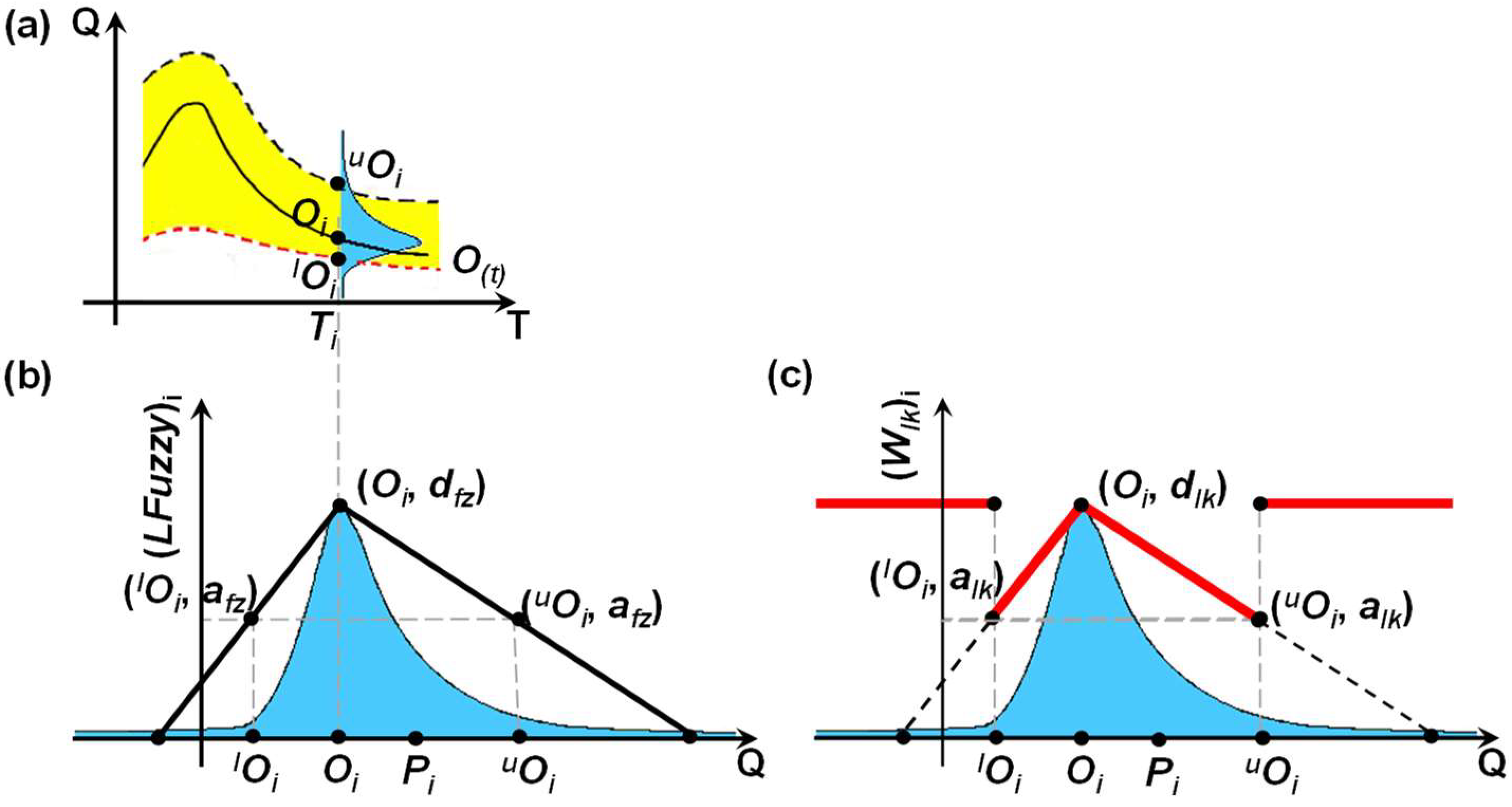
A third likelihood measure that may be used as an alternative to the EF2 or E1 indexes is considered proportional to the linear fuzzy measure (Figure 3) and does not depend on residual values. For a given ith instantaneous Ti (Figure 3a), lOi (lower than Oi) and uOi (greater than Oi) are the ith (data uncertainty) characteristic values associated with Oi. Then, as shown in Figure 3b, any associated distribution density function may be “approximated” through a triangular “linear” fuzzy distribution (LFuzzy) on the basis of the parameters afz and dfz, besides Oi, lOi, and uOi.
Thus, a simple linear equation may be used to assess the value of LFuzzy and, as such, of model performance. It should be noted that, since |Oi − lOi| and |Oi − uOi| may be different, LFuzzy may approximate any skewness present in the original probability density function. Furthermore, since LFuzzy is used as an alternative likelihood measure, dfz adopts the value of 1.0 (while 0 < afz < 1.0), which negates the concept of density function attached to LFuzzy, as the area under the curve is not equal to unity anymore. An arbitrary value of afz = 0.1 was used throughout the study, implying a low likelihood value (i.e., a severe penalty) for Pi departing from Oi, even though not yet out of the data uncertainty band.
The likelihood measure associated with a particular simulation (i.e., to a particular model parameter set) was then defined as the mean value of all of the (LFuzzy)i values corresponding to the different ith instantaneous Ti values that are included in the simulation. Nevertheless, it should be noted that any other type of fuzzy function besides triangular may be used as an alternative likelihood measure. Pragmatically, the linear type is preferred here because it is easier to program.
Thus, any of the above two likelihood measures (EF2 and E1), or any other index that is based on the explicit consideration of residuals, can be used to evaluate model performance, although with no explicit consideration of the discharge data uncertainty. There is then the need of a (simple) procedure to include data uncertainty considerations in the evaluation of model performance using residuals. This could be accomplished, for instance, by using a residual reduction fraction (wlk) since, given the data uncertainty associated with the “observations”, the residual should not be any longer entirely based on the distance between an “observation” and the respective predicted value. Otherwise, we might refuse combinations of model structures and parameters that should be retained and accept others that perhaps are not superior. Ultimately, the aim of the modelling should be to obtain predictions that are within the data uncertainty band rather than obtaining predictions that “match” perfectly “observations” whose values are uncertain.
Hereafter, LFuzzy (Figure 3c) was not only used for calculating a third likelihood measure, but also to define wlk linearly varying within the data uncertainty band. Outside this uncertainty band, however, the traditional definition of the residual was accepted. That is, outside of the data uncertainty band, wlk = 1.0 (Figure 3c). In this context, the relaxed version of the residual was defined as the product of (wlk)i and resi. Then, any model quality index based on residuals, such as EF2 or E1, or any other index which the modeller is familiar with, may be evaluated using this relaxed value of the residual to account for data uncertainty.
Behavioural sets were defined upon a likelihood threshold for the calibration period that, independent of the likelihood measure, was taken equal to 0.5. Upon this prior likelihood distributions, a first prediction band was defined.
More in accordance with the distributed nature of the current hydrological model, a multi-site (MS) validation test [46] was performed using in model validation observations from gauging stations distributed throughout the modelling domain that were not considered during model calibration. This represents a more stringent evaluation of the model as compared to an evaluation based solely on a traditional split-sample (SS) test. MS validation testing has two main implications in the scope of the GLUE methodology. On the one hand, a more relaxed likelihood threshold should be used as compared to the value adopted in a simpler SS test. On the other hand, the likelihood measure that characterises the quality of a particular simulation should be redefined so that the assessment includes predictions at multiple sites (and/or multiple simulated variables).
Hereafter, the likelihood threshold was set as 0.5 for the calibration period. However, if LO(Ωi) = 0.5 (i.e., characterising a behavioural simulation in the calibration period) for a given ith model run and the prediction ability of the model is also the same for the validation period (i.e., LO(Ωi|O) = 0.5), then the numerator of Equation (2) would equal to 0.5 × 0.5 = 0.25, implying a drastic reduction in the resulting likelihood distribution (Lp(Ωi|O)). For this condition, the respective parameter set would not be retained in the analysis (notwithstanding the model has the same predictive ability in the evaluation period as compared to the calibration period). This, therefore, encouraged adopting a likelihood threshold equal to 0.25 for the evaluation period.
Furthermore, a global likelihood measure (GL) was estimated encompassing the predictions for every one of the three gauging (discharge) stations:
In Equation (5), j is a particular parameter set (with j = 1, 2, 3, …, N), m is the total number of (discharge) data stations considered in the analysis, LLk is the local likelihood measure for the kth data station, and wstk is a weighting factor that explains the contribution of LLk to estimate GLj. The term wstk, defined subjectively so that the denominator of Equation (5) equals unity, accounts for data accuracy (uncertainty) and importance of the discharge station in the context of the modelling objectives. Combining these aspects, wstk for m = 3 was (subjectively) given the values 0.15 (Grote Gete), 0.25 (Kleine Gete), and 0.60 (Gete).
3. Results
3.1. Uncertainty Attached to the Stage–Discharge Data
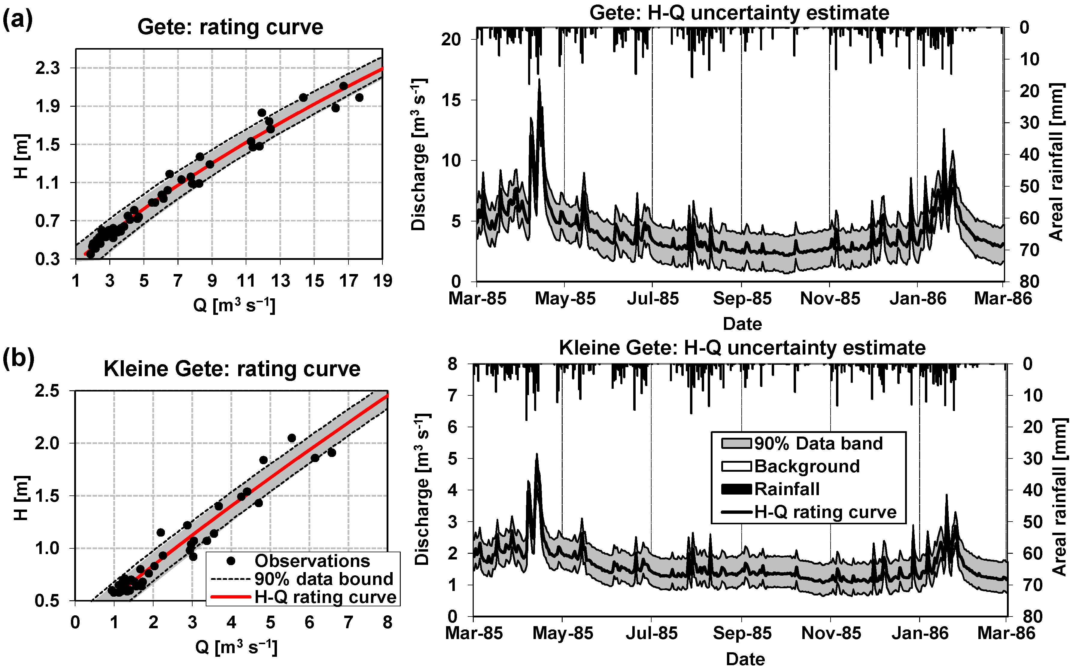
Figure 2 shows the distribution of the sampled points, upon which the rating curves and their associated prediction intervals were derived for both the Gete station (Figure 2a) and the Kleine Gete station (Figure 2b). The figure includes the respective rating curve as well as the prediction interval associated with the curve. The rating curve of the Gete station is Q = −0.0394 + 6.0670(H − 0.10) + 1.1948(H − 0.10)2 with r2 = 0.97; for the Kleine Gete station, the respective regression curve is Q = 3.1873(H − 0.18)1.11208 with r2 = 0.97.
As expected from the total amount of observations and the fact that a relatively good set of peak observations were available to derive the rating curves (Figure 2), the width of the prediction bands is rather uniform along the range of variation of the observed discharge, which is not the common case [6,7,43]. However, this has also been observed in some of the results of Kiang, Gazoorian, McMillan, Coxon, Le Coz, Westerberg, Belleville, Sevrez, Sikorska, Petersen-Øverleir, Reitan, Freer, Renard, Mansanarez, and Mason [34]. The average width of the prediction interval for the Gete station is about 3 m3 s−1. For the Kleine Gete station, this width is approximately 1 m3 s−1. As already stated, a similar and constant discharge uncertainty interval width (i.e., 1.1 m3 s−1) was assumed for the Grote Gete station. The use of the discharge data derived from rating curves for assessing the model performance implies a significant modelling uncertainty that must be addressed at the moment of evaluating model predictions. Figure 2 shows the time evolution of the discharge prediction band throughout the modelling period for these two gauging stations. These hydrographs are plotted along with the areal hyetograph for a visual comparison of the time evolutions of the “observed” discharge and the catchment-areal rainfall.
3.2. Model Calibration, Validation and Sensitivity Analysis
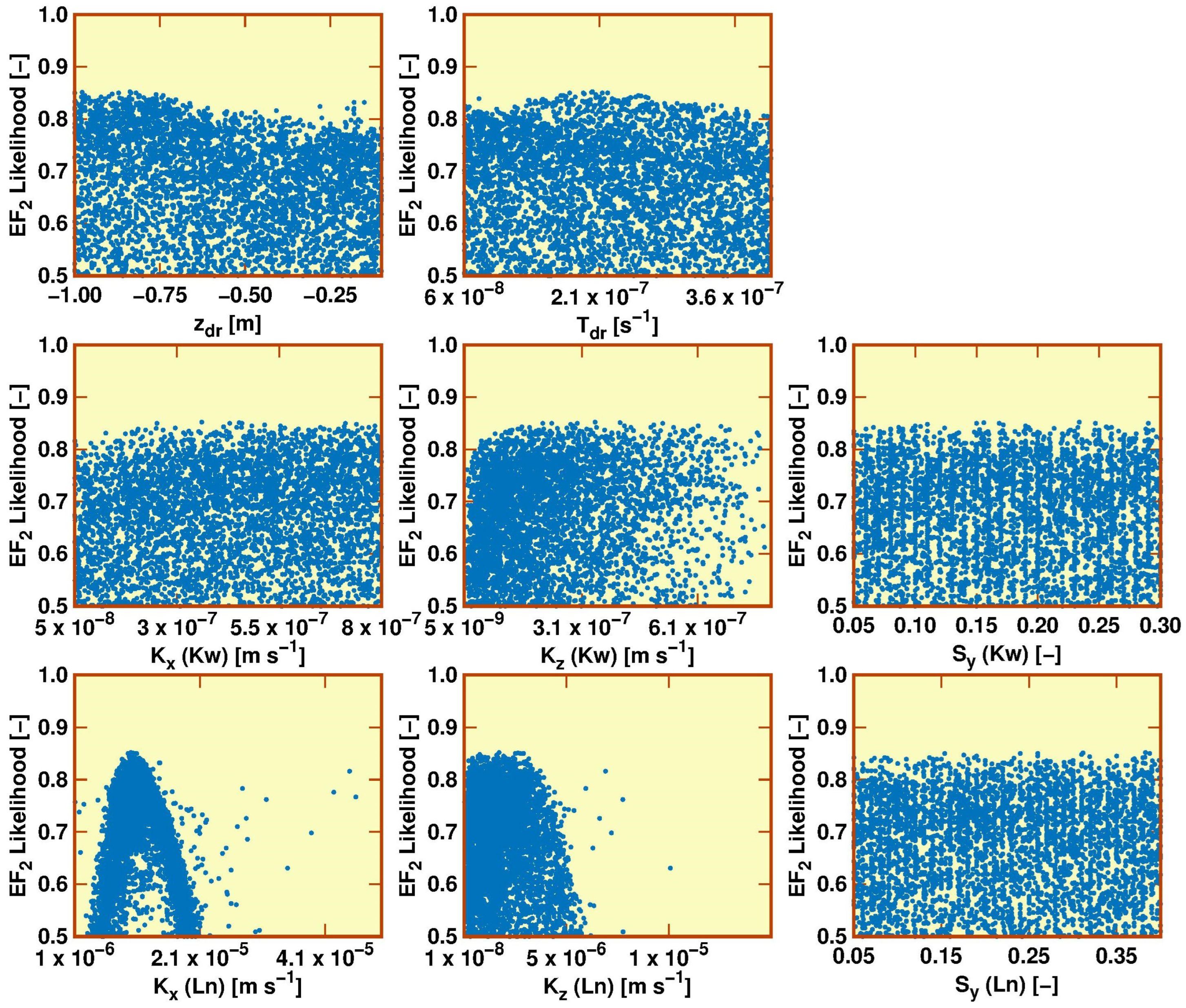
The scatter plots of behavioural parameter sets (target: EF2 = 0.5) are shown in Figure 4 for the calibration period [1 March 1985–31 August 1985]. These were developed after conditioning analysis only on the stream discharges observed at the outlet of the study catchment, without including the analysis of the H-Q data uncertainty. In total, 4234 sets were considered behavioural upon the use of the EF2 index. Out of the 15,000 parameter sets considered, only 47 produced models whose simulations failed due to instabilities.
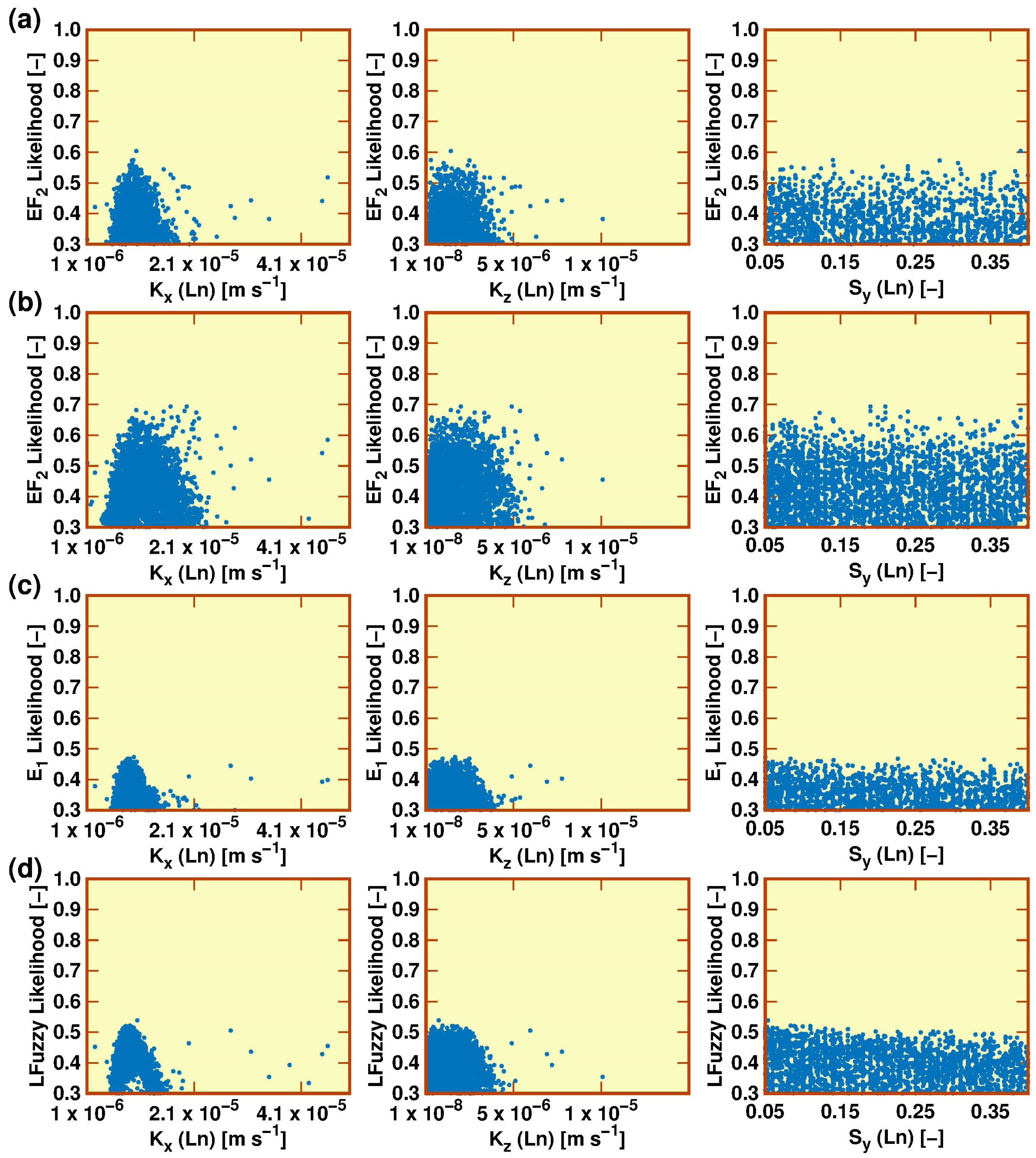
Figure 5 illustrates the scatter plots of behavioural parameter sets for three out of the eight inspected parameters for the validation period (1 September 1985–1 March 1986) (likelihood target of 0.25, although the plots start at the value of 0.30) and after conditioning the analysis on discharges observed at the outlet of the study catchment. These plots were obtained: using the EF2 index and without considering H-Q data uncertainty in the analysis (Figure 5a); using the EF2 index and considering H-Q data uncertainty (Figure 5b); using the E1 index and considering H-Q data uncertainty (Figure 5c); and using LFuzzy and considering H-Q data uncertainty (Figure 5d).
Figure 5 compares the effects of the H-Q data uncertainty on the outcomes of the modelling (i.e., Figure 5a,b), as well as the shape of the parameter distributions as a function of the considered likelihood measure (i.e., Figure 5b–d). The results presented in Figure 5b,c point to the relaxation of the simulation residuals, owing to the H-Q data uncertainty, as explained in the methods section.
Figure 5 shows that, in general, for a given model structure, a consideration of the H-Q data uncertainty in the analysis leads to higher values of the likelihood measures owing to the relaxation of the modelling residual as a function of the H-Q data uncertainty. This, in turn, then leads to a higher number of behavioural simulations (i.e., parameter sets). On the other hand, Figure 5 illustrates that, in general, (i) the trends of the parameter distributions are similar for all of the likelihood measures tested; (ii) there is a significant difference between the magnitudes of the values of the EF2 and E1 model performance coefficients, suggesting that the E1 coefficient is indeed less affected by the correct simulation of some peak flows; and (iii) the magnitudes of the values of the LFuzzy measure are similar to the ones obtained with the E1 index (and the modified concept of modelling residual).
In addition, a comparison of the three lower scatter plots of Figure 4 (for the calibration period) and Figure 5a (for the validation period) reveals the effect of the Bayesian-type update of the parameter distributions. Specifically, there was a significant reduction in the number of behavioural simulations, despite similar shapes of the respective parameter distributions in either simulation period. It should be noted that, for a given model, this reduction takes place in the validation period (i.e., when new observations are available) and does not necessarily represent a reduction in the ability of the model to predict the hydrology of the modelled catchment in the validation period. It is particularly relevant given the implications of the multiplicative form of the numerator of the Bayesian-type update of the parameter distributions (Equation (2)).
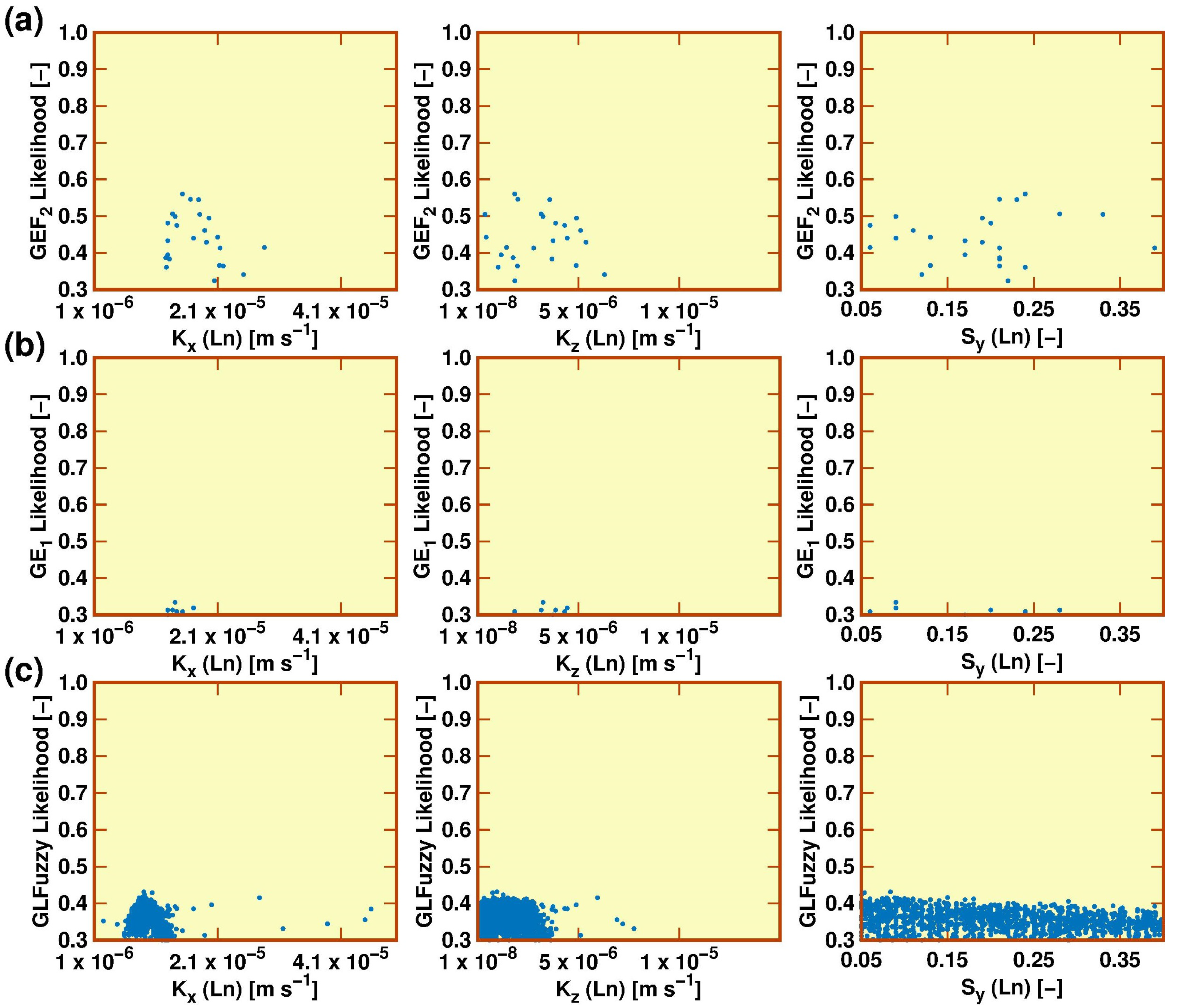
Figure 6 shows the scatter plots of behavioural parameter sets for three of the parameters considered in the validation period with a likelihood target of 0.25, after conditioning the analysis on stream discharges observed at the outlet of the study catchment and at two internal locations (i.e., a multi-site (MS) validation test). These consider the H-Q data uncertainty using the EF2 index (Figure 6a), using the E1 index (Figure 6b), and using LFuzzy (Figure 6c).
Figure 6 illustrates the effect of the distributed evaluation of model performance as a function of likelihood measure used in the current study. Thus, a comparison of Figure 5b–d with Figure 6a–c, respectively, illustrates a marked reduction in the number of behavioural simulations (i.e., of parameter sets) when carrying out the MS validation test relative to traditional validation taking place only at the outlet of the simulated catchment. This is the case when using both the EF2 and E1 indices. Therefore, Figure 6 emphasises that the MS test is normally a more critical evaluation for distributed models. In addition, despite the significant low number of behavioural simulations, the parameter distributions after the MS validation (Figure 6) are practically the same as the ones obtained after traditional validation (Figure 5).
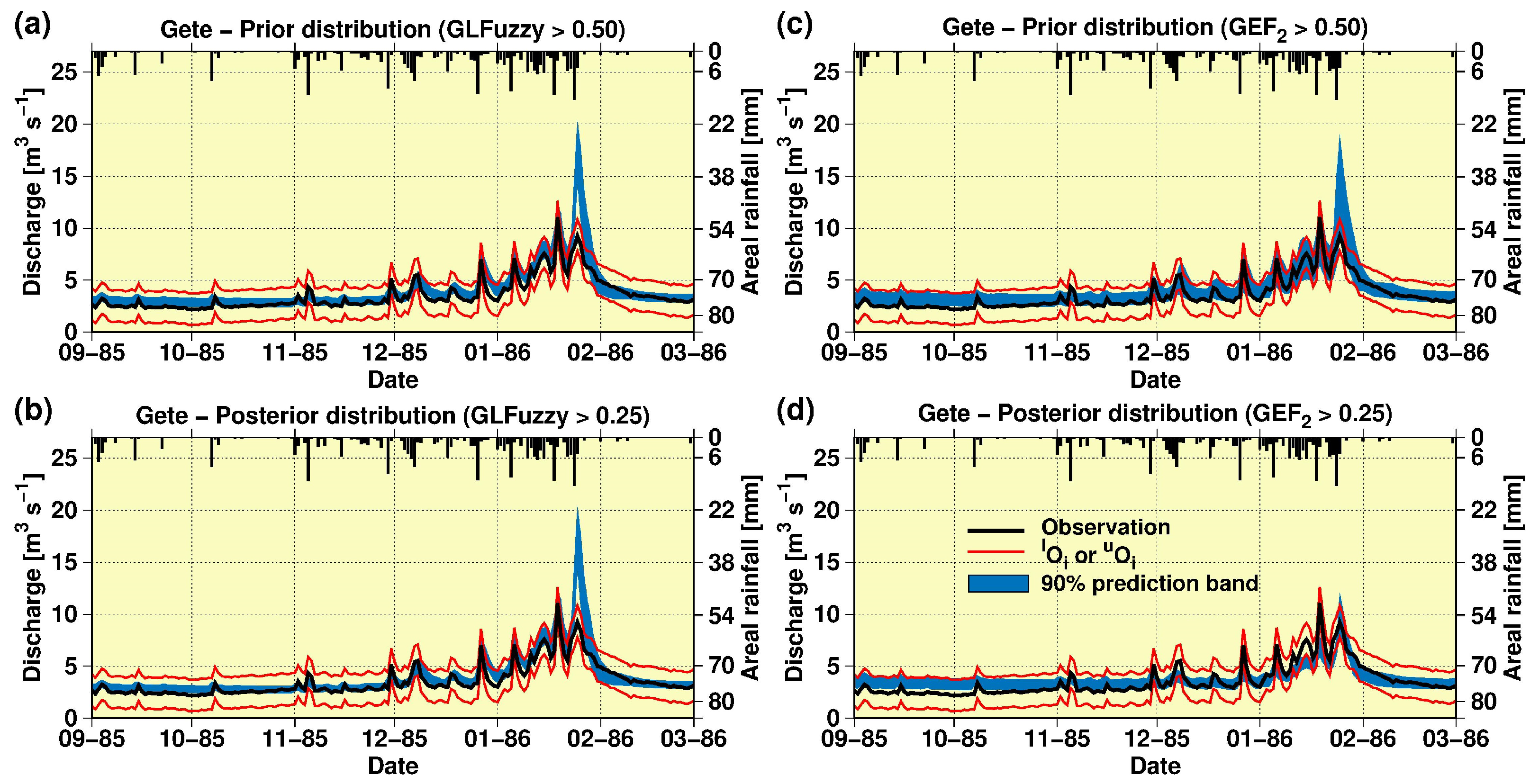
Figure 7 depicts the 90% streamflow prediction limits for the Gete station in the validation period using both prior (likelihood target: 0.50) and posterior (likelihood target: 0.25) likelihood distributions. These are after conditioning based on observed streamflow at the three study gauging stations and considering the H-Q data uncertainty using the LFuzzy likelihood measure (Figure 7a,b) and the EF2 index (Figure 7c,d).
In general, Figure 7 shows the effect of the Bayesian-type update of the prediction band (Equation (2)) on the availability of newer observations for the validation period. Nevertheless, the effect is different as a function of the likelihood measure considered and the approach followed to account for the H-Q data uncertainty. In this context, Figure 7a,b, based on the LFuzzy likelihood measure, depicts only a minimum effect on the width of the prediction band after the application of Equation (2), whilst Figure 7c,d, based on the EF2 likelihood measure and the relaxation of the modelling residuals, shows a significant reduction in the width of the prediction band, after the application of Equation (2).
Furthermore, either prediction band obtained before the application of the Bayesian-type approach (Equation (2)) illustrates that the parameterised MIKE SHE structure had certain problems to simulate the peak event occurring at about the end of January of 1986. This is seen since both the “observed” peak, as well as the respective H-Q uncertainty band, were overestimated by the behavioural simulations. However, once the posterior distribution was defined through the application of Equation (2), Figure 7d based on EF2 and the relaxation of the concept of modelling residuals illustrates that the few remaining behavioural parameterisations of the MIKE SHE structure (i.e., Figure 6a) simulated this peak event without losing that much simulation precision for the rest of events. This is true even though these remaining model parameterisations (26 when EF2 was used or 14 when E1 was used) have a tendency to over-predict low flows.
Collectively, these results imply that (i) expanding the common split-sample single-site evaluation test to a more distributed split-sample multi-site (MS) test, (ii) relaxing the traditional concept of modelling residuals, and (iii) applying the Bayesian-type update of the likelihood distribution, contributed to a better identification of the MIKE SHE parameterisations. Furthermore, these parameterisations were able to simulate the hydrological dynamics of the study catchment within the limits of data uncertainty. This is seen as the prediction band is bracketed in turn by the H-Q data uncertainty band throughout the whole extent of the validation period (even for low flows).
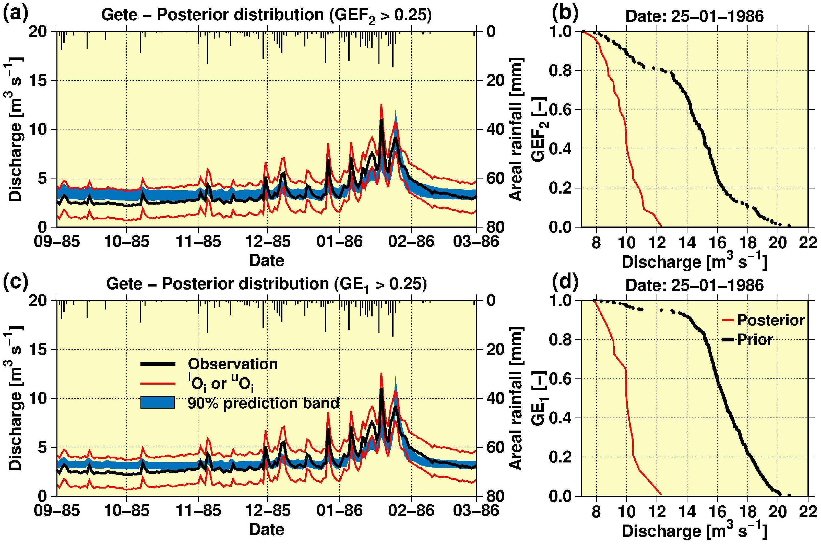
Furthermore, Figure 8 shows the 90% streamflow prediction limits for the Gete gauging station (posterior likelihood distribution) in the validation period after conditioning based on observed streamflow at the three study gauging stations (i.e., the multi-site test) in light of H-Q data uncertainty. Figure 8 also had the respective likelihood cumulative prior and posterior distributions on 25 January 1986 (Figure 8a,b) using the EF2 likelihood measure and (Figure 8c,d) using the E1 likelihood measure.
Figure 8 emphasises that the use of either EF2 or E1 indices by relaxing the traditional concept of modelling residuals to account for H-Q data uncertainty contributed to a better identification of the MIKE SHE parameterisations that can simulate the peak discharge in January 1986 (Figure 8a,c). Namely, once Equation (2) was applied, the likelihood distributions (Figure 8b,d) were significantly modified on 25 January 1986, such that the range of the respective (discharge) prediction band was markedly reduced. For instance, Figure 8b, based on EF2, depicts that the prediction range for the prior likelihood distribution, i.e., [~7.0, ~21.0] m3 s−1, was drastically reduced to [~7.0, ~12.2] m3 s−1 for the posterior distribution.
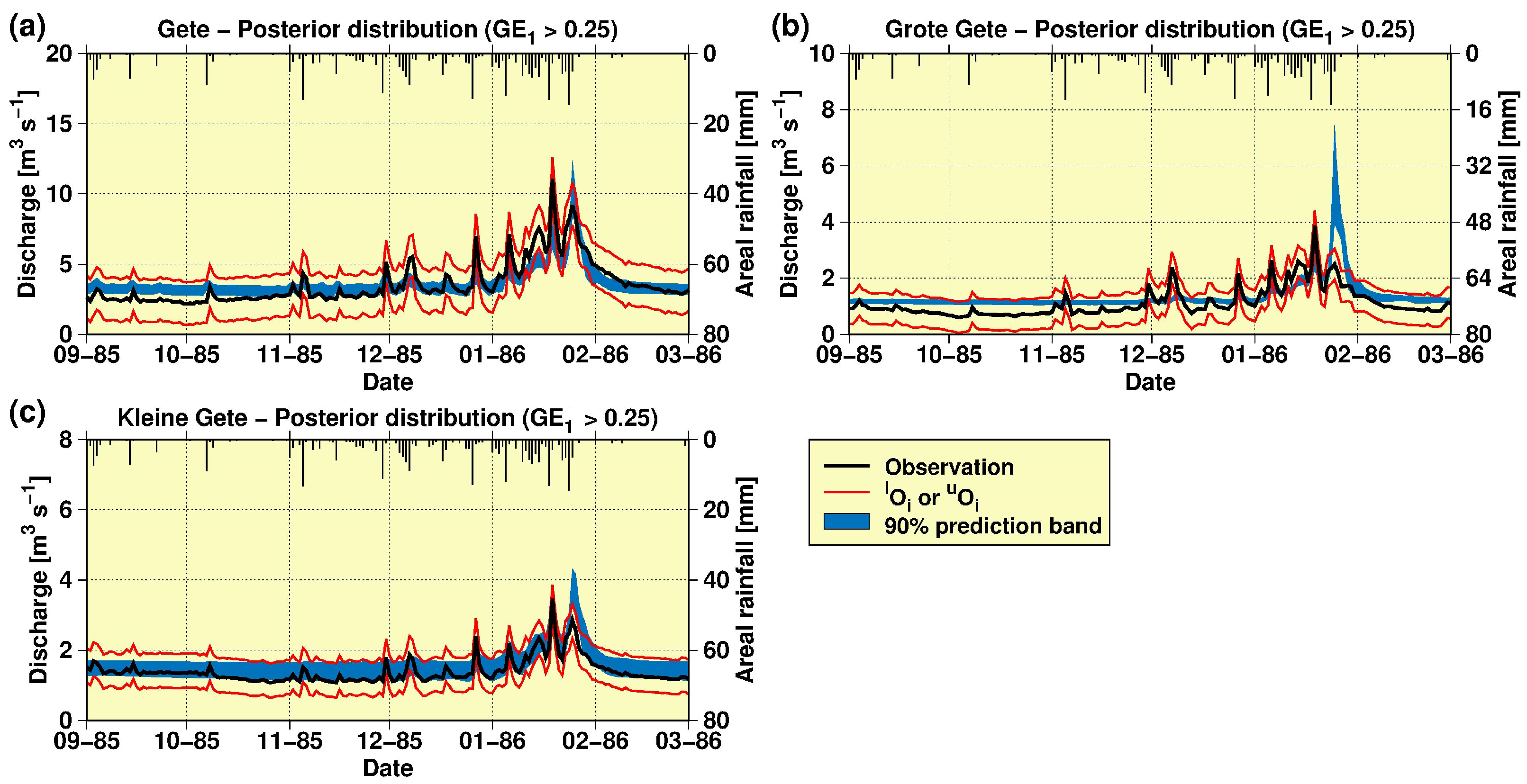
With respect to the MS validation test and the individual contribution of the two internal stations to the overall simulation at the outlet of the catchment, Figure 9 illustrates the 90% streamflow prediction limits in the validation period using the E1 measure and the posterior likelihood distribution after conditioning based on observed streamflow at the three gauging stations and considering the H-Q data uncertainty for the Gete station (Figure 9a); the Grote Gete station (Figure 9b); and the Kleine Gete station (Figure 9c). The results depicted in Figure 9 are similar to those obtained on the basis of the EF2 index. Figure 9b illustrates that the parameterised MIKE SHE structure had higher difficulties to model the discharge at the Grote Gete station, which is located in the mid-part of the study catchment (Figure 1). This difficulty was seen particularly for the peak recorded on 25 January 1986, but also the antecedent base flows. The peak flow was simulated much better for the Kleine Gete station and (as already discussed) for the Gete station. Since both stations are near to each other (Figure 1), the better simulation recorded for the Kleine Gete station compensated the overestimations recorded for the upper Grote Gete station.
Nevertheless, despite the stricter MS validation test and narrow calibration and validation periods used in this study, Figure 9 emphasises that, globally, the few remaining behavioural parameterisations of MIKE SHE are able to simulate the hydrological dynamics of the study catchment within the data uncertainty constraints.
4. Discussion
The purpose of this research was not to explicitly or formally compare the current suggested approach to others proposed in the literature. Rather, our aim was to propose a simpler method (in terms of stochastic complexity) than the ones reported in the literature. The goal was to develop a method so that both practitioners and non-expert researchers could explicitly assess the effects of discharge uncertainties upon hydrological predictions without the need of complicated calculations. It is believed that the approach developed uses a stochastic framework that is rather simpler than the ones reported in the literature.
It is worth noting that the parametric approach followed in this study to define the H-Q data uncertainty bands is simple relative to other methods reported in the literature, which is in line with the aim of the current research. Other simple approaches could be used with the same purpose in mind. Of course, different approaches would produce different H-Q data uncertainty magnitudes. For instance, the non-parametric LOESS regression [18] could be applied. Although the respective results are not shown herein, the prediction bands associated with LOESS analysis carried out on the data of the Gete and Kleine Gete stations suggested slightly wider uncertainty bands than the ones finally adopted in this study.
In this context, the congruency of the H-Q uncertainty estimates should be continuously monitored to provide constant feedback that incorporates newly available field H-Q measures. Such monitoring will confirm (or not) the appropriateness of the approach initially used to derive uncertainty estimates. In addition, more complex statistical frameworks (i.e., [2,15,16,17,20,21,22,24,26,29,30,31,32,33,34]), some of which take explicitly into account the rating curve shape uncertainty but are not free of subjective assumptions such as normality of errors or permanent/uniform river flow, could be incorporated at this initial stage of the proposed approach for deriving H-Q data uncertainty estimates. This would not interfere with the current approach for model evaluation explicitly incorporating H-Q data uncertainty estimates and conditioning the analysis on distributed model predictions.
Furthermore, the reformulation of the concept of modelling residual provides a statistical measure that the modeller is familiar with rather than adopting or programming a newer, unfamiliar, and too-specific metric. The latter approach has been adopted in previous work [33,58] that suggested using statistically complex novel metrics that are, however, not suitable [33] for assessing other types of modelling than in the exclusive context of assessing the effects of discharge uncertainty. Our approach does not have this pitfall since the adopted metrics can be used in the scope of any modelling assessment.
Although the overall approach presented in this study is similar to the overall approaches of previously published works, such as [2,33,45,58,59], there are significant differences. For instance, (i) the continuous hydrograph simulation rather than only peak simulation was considered; (ii) a multi-site rather than a single-site validation scheme was applied; (iii) the approach was not bound to the use of a given rainfall-runoff code; and (iv) a far much simpler stochastic framework was implemented. The latter is definitively a differentiating feature that would not only enable using simple rainfall-runoff models (i.e., [2,33,58]), but also complex ones (as done in this study). In this regard, even [2] concludes that, contrary to their initial premise, a complex stochastic assessment may not be really justified for operational purposes, which is in line with the original purpose of the present research.
Furthermore, it must be emphasised that although GLUE has been used in this study to outline the model prediction bands, the reader is free to use different and perhaps statistically more rigorous approaches (e.g., [2,27,28,59]). The suggested model evaluation approach is not bound to GLUE. Nevertheless, GLUE was preferred in this study, not only because it is easier to implement than more statistically formal Bayesian approaches or complex optimisation processes, but also because, contrarily to what is sometimes stated in related research (i.e., [58]), any model performance measure could (subjectively) be used (i.e., which the modeller is familiar with), as long as appropriate re-scaling takes place to treat those measures as likelihoods (as done in this study). GLUE is not bound to the EF2 index (sometimes termed as NSE in related research). In addition, GLUE does not need to be strictly Bayesian-type in nature [54].
The different scatter plots (dotty plots) demonstrated that most of the studied parameters, except the hydraulic conductivity of the Ln layer, were insensitive to the model predictions (flat-topped scatter plots). This agrees with previous studies on the modelling of the study catchment [52,54]. In principle, these results confirm the presence of equifinality as it was not feasible to identify a single optimal parameter set for the model of the study site (see, for instance, Figure 6), which is also in line with results of past studies. However, a remarkable aspect in this study is that only a few parameter sets, 26 when EF2 was used or 14 when E1 was used, were left after the Bayesian-type update of the prior likelihood distribution.
Despite GLUE receiving considerable criticism that has focussed on the subjective assumptions required, particularly in choosing a likelihood measure, avoiding the adoption of a formal error model, and ending up with model prediction bands that are conditional on those subjective assumptions [27,28,56,60,61], the method was implemented in this current study precisely because of this feasibility of incorporating subjective assumptions into the process for estimating model prediction bands. Within this framework, likelihood measures were easily (i.e., subjectively) adapted to account for multi-site evaluation of predictions, as well as for discharge uncertainty. In this regard, adopting an error model might be hard to achieve for real hydrological modelling applications without adopting statistical assumptions that are difficult to reach under real conditions [60]. Clearly, we would (i.e., subjectively) choose a model performance measure that reflects the real information content in some way. After all, this choice would be transparent and, consequently, open to discussion. However, formal statistical likelihood measures require assumptions about the distribution of errors, which are rarely matched in hydrological modelling. Nevertheless, GLUE could use such approaches as special cases if justifiable [56].
Furthermore, owing to some constrains, including model license and practical issues, the current study has focused only on the uncertainty associated with one of the several data types used in hydrological modelling without considering explicitly the uncertainties from other sources, including other modelling data and model structure. These uncertainties are globally taken into consideration when applying the GLUE methodology for defining prediction bands by mapping them onto parameter uncertainty, which might lead to some bias when estimating the prediction bands. This incomplete (i.e., non-explicit) understanding of the different uncertainties accentuates the imperfection of our hydrological models. Nevertheless, for diagnostic or operational purposes, this paper takes one step towards highlighting data uncertainties in a simple manner so that decision making, carried out by practitioners far from rigorous scientific studies, may benefit from predictions from these models.
Finally, it is likely that the short duration of the warming-up, calibration, and evaluation periods played a significant role in the overall quality of the current model predictions. Definitively, much longer calibration periods encompassing several four-season events are advisable. This was not feasible in this study owing to computing and model license constraints. Nevertheless, it is believed that the main conclusions of this study are independent of the general quality of the model predictions and are applicable when using other models than MIKE SHE and/or under other modelling conditions, especially if discharge (and/or other output variable) data uncertainty observations or estimates are available for the modelling.
It is believed that further research should focus on improving and standardising similar approaches for evaluating data uncertainty and their effects on model predictions. This would allow adapting model evaluation strategies, allowing for more suitable model parameterisations and/or structures to be identified for the study catchment/conditions. Research should also focus on not only reducing the data uncertainty effects on the selection of the most suitable model parameterisations/structures, but also the data uncertainty itself by modifying or adapting both monitoring and modelling protocols. In this context, besides improving accuracy of field data collection campaigns, modelling protocols should expand already ongoing practices, such as basing model prediction and evaluation, on the use of stages rather than on discharges [1,62,63]. For that, simulation codes should enable the modeller to choose this option for rainfall-stage modelling, and meteorological services in general should review their procedures to report the rating curve data, the original stage data, and the respective estimated discharges. Unfortunately, such reporting is not usually the case, particularly in developing countries.
Future research should also focus on analysing the potential effects that other variables, such as topography/slope and discharge estimation/surveying approaches, might have on discharge data and, ultimately, on hydrological modelling. This would be of interest for modelling applications in mountainous regions, particularly in developing countries where there is a scarcity of hydro-meteorological data and/or where a lack of free access to appropriate information may constrain the development of operative models that respond acceptably to data uncertainties.
5. Conclusions
The effect of the uncertainty associated with stage-derived discharge on the prediction bands of a distributed hydrological modelling for an agricultural, medium-sized catchment was assessed. The analysis of the observations used to derive the rating curves for the gauging stations depicted significant uncertainty in the resulting rating curves and associated discharge “observations”. The estimated uncertainty levels, however, were remarkably regular throughout the rating curves, showing no significant accentuation for higher discharges.
Explicitly considering this data uncertainty during model evaluation resulted in more parameterisations of the MIKE SHE-based model being acceptable for simulating the study catchment—of course, within the limitations of the observations. This was seen independent of the likelihood measure considered. Furthermore, our study revealed that the shapes of the distributions of the eight model parameters inspected are consistent despite the likelihood measure being considered.
The distributed multi-site (MS) evaluation of the discharge predictions drastically reduced the number of parameterisations of the MIKE SHE-based model that were considered as acceptable for simulating the study catchment. This was particularly evident for the gauging station, for which no original stage–discharge data was available. Results showed that the remaining MIKE SHE parameterisations were capable of modelling a particular peak event (at the outlet of the catchment) that was otherwise overestimated by the rest of the model parameterisations.
The latter analysis did not only depict the importance and effect of the MS test in distributed catchment modelling evaluation, but also emphasised that, within the scope of the traditional GLUE approach, the resulting model performance band depends on the likelihood measure and approach to consider the discharge data uncertainty in model evaluation. In the current study, a redefinition of the concept of modelling residual in the context of commonly used model performance indices, such as [57], the Nash and Sutcliffe EF2, and its alternative E1, proved to be more effective than the use of a linear fuzzy measure of likelihood. Of course, this has significance specific to coping with data uncertainties when selecting the most appropriate model parameterisations under the current discharge data uncertainty constraints.
Finally, the main message of this paper is that practitioners (and non-expert researchers, too) should be aware of the importance of carrying out uncertainty analyses of streamflow data—even when carried out in a very simple way. Such simple approaches, rather than those complex approaches often presented in research (i.e., as depicted in this study), could help in making appropriate (i.e., more robust) decisions based on more realistic modelling predictions and, as such, improve the effectiveness of water management applications.
Author Contributions
Conceptualisation, R.F.V.; methodology, R.F.V.; validation, R.F.V. and H.H.; formal analysis, R.F.V.; investigation, R.F.V. and H.H.; resources, R.F.V. and H.H.; writing—original draft preparation, R.F.V.; writing—review and editing, R.F.V. and H.H.; visualization, R.F.V. and H.H.; supervision, R.F.V. and H.H.; project administration, R.F.V. and H.H.; funding acquisition, R.F.V. and H.H. All authors have read and agreed to the published version of the manuscript.
Funding
The VLIR-UOS Biodiversity Network Ecuador kindly covered the Article Production Costs (APC).
Institutional Review Board Statement
Not applicable.
Informed Consent Statement
Not applicable.
Data Availability Statement
Restrictions apply to the availability of data used in this research. Data was obtained from several public Belgian institutions and might be available directly from them. These institutions include: the Department Water of AMINAL, DIHO; OC GIS-Vlaanderen; the Royal Meteorological Institute of Belgium; the Flemish Community Department Afdeling Natuurlijke Rijkdommen en Energie; the Laboratory of Hydrogeology and the former Institute of Soil and Water Management of the KULeuven; the Belgian Geological Survey; Le Ministère de la Region Wallone, Direction Générale des Resources Naturelles et de l’Environment, Division d’Eau, Service des Eaux Souterraines and the Centre d’Environment, Université de Liège.
Acknowledgments
The research was executed as part of the VLIR-UOS Biodiversity Network Ecuador. The authors are thankful to the three anonymous reviewers and to Steve Lyon for their constructive suggestions and corrections that helped enhancing the shape of the current manuscript.
Conflicts of Interest
The authors declare no conflict of interest. The funders had no role in the design of the study; in the collection, analyses, or interpretation of data; in the writing of the manuscript, or in the decision to publish the results.
References
- Sikorska, A.E.; Renard, B. Calibrating a hydrological model in stage space to account for rating curve uncertainties: General framework and key challenges. Adv. Water Resour. 2017, 105, 51–66. [Google Scholar] [CrossRef] [Green Version]
- Ocio, D.; Le Vine, N.; Westerberg, I.; Pappenberger, F.; Buytaert, W. The role of rating curve uncertainty in real-time flood forecasting. Water Resour. Res. 2017, 53, 4197–4213. [Google Scholar] [CrossRef] [Green Version]
- Chen, Y.-C.; Kuo, J.-J.; Yu, S.-R.; Liao, Y.-J.; Yang, H.-C. Discharge Estimation in a Lined Canal Using Information Entropy. Entropy 2014, 16, 1728–1742. [Google Scholar] [CrossRef] [Green Version]
- McMillan, H.; Seibert, J.; Petersen-Overleir, A.; Lang, M.; White, P.; Snelder, T.; Rutherford, K.; Krueger, T.; Mason, R.; Kiang, J. How uncertainty analysis of streamflow data can reduce costs and promote robust decisions in water management applications. Water Resour. Res. 2017, 53, 5220–5228. [Google Scholar] [CrossRef] [Green Version]
- Shah, M.A.A.; Anwar, A.A.; Bell, A.R.; ul Haq, Z. Equity in a tertiary canal of the Indus Basin Irrigation System (IBIS). Agric. Water Manag. 2016, 178, 201–214. [Google Scholar] [CrossRef]
- Sivapragasam, C.; Muttil, N. Discharge Rating Curve Extension—A New Approach. Water Resour. Manag. 2005, 19, 505–520. [Google Scholar] [CrossRef]
- Lang, M.; Pobanz, K.; Renard, B.; Renouf1, E.; Sauquet, E. Extrapolation of rating curves by hydraulic modelling, with application to flood frequency analysis. Hydrol. Sci. J. 2010, 55, 883–898. [Google Scholar] [CrossRef] [Green Version]
- Westerberg, I.K.; McMillan, H.K. Uncertainty in hydrological signatures. Hydrol. Earth Syst. Sci. 2015, 19, 3951–3968. [Google Scholar] [CrossRef] [Green Version]
- Refsgaard, J.C.; Stisen, S.; Koch, J. Hydrological process knowledge in catchment modelling—Lessons and perspectives from 60 years development. Hydrol. Processes 2022, 36, e14463. [Google Scholar] [CrossRef]
- Gravelle, R. Discharge Estimation: Techniques and Equipment. In Geomorphological Techniques; Cook, S.J., Clarke, L.E., Nield, J.M., Eds.; British Society for Geomorphology: London, UK, 2015; Volume 3, pp. 1–8. [Google Scholar]
- Muste, M.; Hoitink, T. Measuring Flood Discharge; Oxford Research Encyclopedia of Natural Hazar: Oxford, UK, 2017. [Google Scholar]
- Pedersen, Ø.; Rüther, N. Hybrid modelling of a gauging station rating curve. Procedia Eng. 2016, 154, 433–440. [Google Scholar] [CrossRef] [Green Version]
- Tsubaki, R.; Fujita, I.; Tsutsumi, S. Measurement of the flood discharge of a small-sized river using an existing digital video recording system. J. Hydro-Environ. Res. 2011, 5, 313–321. [Google Scholar] [CrossRef] [Green Version]
- Habib, E.H.; Meselhe, E.A. Stage–Discharge Relations for Low-Gradient Tidal Streams Using Data-Driven Models. J. Hydraul. Eng. 2006, 132, 482–492. [Google Scholar] [CrossRef] [Green Version]
- Petersen-Øverleir, A. Modelling stage–discharge relationships affected by hysteresis using the Jones formula and nonlinear regression. Hydrol. Sci. J. 2006, 51, 365–388. [Google Scholar] [CrossRef] [Green Version]
- Garcia, R.; Costa, V.; Silva, F. Bayesian Rating Curve Modeling: Alternative Error Model to Improve Low-Flow Uncertainty Estimation. J. Hydrol. Eng. 2020, 25, 04020012. [Google Scholar] [CrossRef]
- Pedersen, Ø.; Aberle, J.; Rüther, N. Hydraulic scale modelling of the rating curve for a gauging station with challenging geometry. Hydrol. Res. 2019, 50, 825–836. [Google Scholar] [CrossRef]
- Coxon, G.; Freer, J.; Westerberg, I.K.; Wagener, T.; Woods, R.; Smith, P.J. A novel framework for discharge uncertainty quantification applied to 500 UK gauging stations. Water Resour. Res. 2015, 51, 5531–5546. [Google Scholar] [CrossRef] [PubMed] [Green Version]
- Westerberg, I.; Guerrero, J.-L.; Seibert, J.; Beven, K.J.; Halldin, S. Stage-discharge uncertainty derived with a non-stationary rating curve in the Choluteca River, Honduras. Hydrol. Processes 2011, 25, 603–613. [Google Scholar] [CrossRef]
- Qiu, J.; Liu, B.; Yu, X.; Yang, Z. Combining a segmentation procedure and the BaRatin stationary model to estimate nonstationary rating curves and the associated uncertainties. J. Hydrol. 2021, 597, 126168. [Google Scholar] [CrossRef]
- Morlot, T.; Perret, C.; Favre, A.-C.; Jalbert, J. Dynamic rating curve assessment for hydrometric stations and computation of the associated uncertainties: Quality and station management indicators. J. Hydrol. 2014, 517, 173–186. [Google Scholar] [CrossRef] [Green Version]
- Shao, Q.; Dutta, D.; Karim, F.; Petheram, C. A method for extending stage-discharge relationships using a hydrodynamic model and quantifying the associated uncertainty. J. Hydrol. 2018, 556, 154–172. [Google Scholar] [CrossRef]
- van der Keur, P.; Henriksen, H.J.; Refsgaard, J.C.; Brugnach, M.; Pahl-Wostl, C.; Dewulf, A.; Buiteveld, H. Identification of Major Sources of Uncertainty in Current IWRM Practice. Illustrated for the Rhine Basin. Water Resour. Manag. 2008, 22, 1677–1708. [Google Scholar] [CrossRef]
- Baldassarre, G.; Montanari, A. Uncertainty in river discharge observations: A quantitative analysis. Hydrol. Earth Syst. Sci. 2009, 13, 913–921. [Google Scholar] [CrossRef] [Green Version]
- Bales, J.D.; Wagner, C.R. Sources of uncertainty in flood inundation maps. J. Flood Risk Manag. 2009, 2, 139–147. [Google Scholar] [CrossRef]
- Le Coz, J.; Renard, B.; Bonnifait, L.; Branger, F.; Le Boursicaud, R. Combining hydraulic knowledge and uncertain gaugings in the estimation of hydrometric rating curves: A Bayesian approach. J. Hydrol. 2014, 509, 573–587. [Google Scholar] [CrossRef] [Green Version]
- Moges, E.; Demissie, Y.; Larsen, L.; Yassin, F. Review: Sources of Hydrological Model Uncertainties and Advances in Their Analysis. Water 2021, 13, 28. [Google Scholar] [CrossRef]
- Papacharalampous, G.; Tyralis, H.; Koutsoyiannis, D.; Montanari, A. Quantification of predictive uncertainty in hydrological modelling by harnessing the wisdom of the crowd: A large-sample experiment at monthly timescale. Adv. Water Resour. 2020, 136, 103470. [Google Scholar] [CrossRef] [Green Version]
- Petersen-Øverleir, A.; Soot, A.; Reitan, T. Bayesian Rating Curve Inference as a Streamflow Data Quality Assessment Tool. Water Resour. Manag. 2009, 23, 1835–1842. [Google Scholar] [CrossRef]
- Singh, V.P.; Cui, H.; Byrd, A.R. Derivation of rating curve by the Tsallis entropy. J. Hydrol. 2014, 513, 342–352. [Google Scholar] [CrossRef]
- Barbetta, S.; Moramarco, T.; Perumal, M. A Muskingum-based methodology for river discharge estimation and rating curve development under significant lateral inflow conditions. J. Hydrol. 2017, 554, 216–232. [Google Scholar] [CrossRef]
- Horner, I.; Renard, B.; Le Coz, J.; Branger, F.; McMillan, H.K.; Pierrefeu, G. Impact of Stage Measurement Errors on Streamflow Uncertainty. Water Resour. Res. 2018, 54, 1952–1976. [Google Scholar] [CrossRef] [Green Version]
- Westerberg, I.K.; Sikorska-Senoner, A.E.; Viviroli, D.; Vis, M.; Seibert, J. Hydrological model calibration with uncertain discharge data. Hydrol. Sci. J. 2020. [Google Scholar] [CrossRef]
- Kiang, J.E.; Gazoorian, C.; McMillan, H.; Coxon, G.; Le Coz, J.; Westerberg, I.K.; Belleville, A.; Sevrez, D.; Sikorska, A.E.; Petersen-Øverleir, A.; et al. A Comparison of Methods for Streamflow Uncertainty Estimation. Water Resour. Res. 2018, 54, 7149–7176. [Google Scholar] [CrossRef] [Green Version]
- Muñoz, P.; Orellana-Alvear, J.; Bendix, J.; Feyen, J.; Célleri, R. Flood Early Warning Systems Using Machine Learning Techniques: The Case of the Tomebamba Catchment at the Southern Andes of Ecuador. Hydrology 2021, 8, 183. [Google Scholar] [CrossRef]
- Nanding, N.; Rico-Ramirez, M.A.; Han, D.; Wu, H.; Dai, Q.; Zhang, J. Uncertainty assessment of radar-raingauge merged rainfall estimates in river discharge simulations. J. Hydrol. 2021, 603, 127093. [Google Scholar] [CrossRef]
- Aronica, G.T.; Candela, A.; Viola, F.; Cannarozzo, M. Influence of rating curve uncertainty on daily rainfall–runoff model predictions. In Proceedings of the Seventh IAHS Scientific Assembly, Foz do Iguacu, Brazil, 3–9 April 2005; pp. 116–124. [Google Scholar]
- Pappenberger, F.; Matgen, P.; Beven, K.J.; Henry, J.-B.; Pfister, L.; de Fraipont, P. Influence of uncertain boundary conditions and model structure on flood inundation predictions. Adv. Water Resour. 2006, 29, 1430–1449. [Google Scholar] [CrossRef]
- Huard, D.; Mailhot, A. Calibration of hydrological model GR2M using Bayesian uncertainty analysis. Water Resour. Res. 2008, 44, W02424. [Google Scholar] [CrossRef] [Green Version]
- Liu, Y.L.; Freer, J.; Beven, K.; Matgen, P. Towards a limits of acceptability approach to the calibration of hydrological models: Extending observation error. J. Hydrol. 2009, 367, 93–103. [Google Scholar] [CrossRef]
- Krueger, T.; Freer, J.; Quinton, J.N.; Macleod, C.J.A.; Bilotta, G.S.; Brazier, R.; Butler, P.; Haygarth, P. Ensemble evaluation of hydrological model hypotheses. Water Resour. Res. 2010, 46, W07516. [Google Scholar] [CrossRef]
- McMillan, H.; Freer, J.; Pappenberger, F.; Krueger, T.; Clark, M. Impacts of uncertain river flow data on rainfall-runoff model calibration and discharge predictions. Hydrol. Processes 2010, 24, 1270–1284. [Google Scholar] [CrossRef]
- Domeneghetti, A.; Castellarin, A.; Brath, A. Assessing rating-curve uncertainty and its effects on hydraulic model calibration. Hydrol. Earth Syst. Sci. 2012, 16, 1191–1202. [Google Scholar] [CrossRef] [Green Version]
- Bermudez, M.; Neal, J.C.; Bates, P.D.; Coxon, G.; Freer, J.E.; Cea, L.; Puertas, J. Quantifying local rainfall dynamics and uncertain boundary conditions into a nested regional-local flood modeling system. Water Resour. Res. 2017, 53, 2770–2785. [Google Scholar] [CrossRef] [Green Version]
- Kastali, A.; Zeroual, A.; Zeroual, S.; Hamitouche, Y. Auto-calibration of HEC-HMS Model for Historic Flood Event under Rating Curve Uncertainty. Case Study: Allala Watershed, Algeria. KSCE J. Civ. Eng. 2022, 26, 482–493. [Google Scholar] [CrossRef]
- Vázquez, R.F.; Feyen, L.; Feyen, J.; Refsgaard, J.C. Effect of grid-size on effective parameters and model performance of the MIKE SHE code applied to a medium sized catchment. Hydrol. Processes 2002, 16, 355–372. [Google Scholar] [CrossRef]
- Van Poucke, L.; Verhoeven, R. Onderzoek Naar de Relatie Debiet—Waterpeil, Het Schatten van Ontbrekende Gegevens en Verwerking van de Gegevens van de Hydrometrische Stations van de Afdeling Water, Administratie Milieu-, Natuur-, Land- en Waterbeheer, Ministerie van de Vlaamse Gemeenschap (Dienstjaar 1995); Universiteit Gent, Laboratorium voor Hydraulica: Gent, Belgium, 1996. [Google Scholar]
- Vázquez, R.F.; Feyen, J. Effect of potential evapotranspiration estimates on effective parameters and performance of the MIKE SHE-code applied to a medium-size catchment. J. Hydrol. 2003, 270, 309–327. [Google Scholar] [CrossRef]
- DHI. MIKE-SHE v. 5.30 User Guide and Technical Reference Manual; Danish Hydraulic Institute: Horsholm, Denmark, 1998; p. 50. [Google Scholar]
- Christiaens, K.; Feyen, J. Constraining soil hydraulic parameter and output uncertainty of the distributed hydrological MIKE SHE model using the GLUE framework. Hydrol. Processes 2002, 16, 373–391. [Google Scholar] [CrossRef]
- Daneshmand, H.; Alaghmand, S.; Camporese, M.; Talei, A.; Daly, E. Water and salt balance modelling of intermittent catchments using a physically-based integrated model. J. Hydrol. 2019, 568, 1017–1030. [Google Scholar] [CrossRef]
- Vázquez, R.F.; Hampel, H. Prediction limits of a catchment hydrological model using different estimates of ETp. J. Hydrol. 2014, 513, 216–228. [Google Scholar] [CrossRef]
- Janert, P.K. Gnuplot in Action, 2nd ed.; Manning Publications Co.: New York, NY, USA, 2016; p. 372. [Google Scholar]
- Vázquez, R.F.; Beven, K.; Feyen, J. GLUE based assessment on the overall predictions of a MIKE SHE application. Water Resour. Manag. 2009, 23, 1325–1349. [Google Scholar] [CrossRef]
- Haan, C.T.; Barfield, B.J.; Hayes, J.C. (Eds.) Design Hydrology and Sedimentology for Small Catchments; Harcourt Brace & Company: San Diego, CA, USA, 1994; p. 587. [Google Scholar]
- Beven, K.J.; Binley, A. GLUE: 20 years on. Hydrol. Processes 2014, 28, 5897–5918. [Google Scholar] [CrossRef] [Green Version]
- Legates, D.R.; McCabe, G.J. Evaluating the use of “goodness-of-fit” measures in hydrological and hydroclimatic model validation. Water Resour. Res. 1999, 35, 233–241. [Google Scholar] [CrossRef]
- Douinot, A.; Roux, H.; Dartus, D. Modelling errors calculation adapted to rainfall—Runoff model user expectations and discharge data uncertainties. Environ. Model. Softw. 2017, 90, 157–166. [Google Scholar] [CrossRef] [Green Version]
- Sellami, H.; La Jeunesse, I.; Benabdallah, S.; Vanclooster, M. Parameter and rating curve uncertainty propagation analysis of the SWAT model for two small Mediterranean catchments. Hydrol. Sci. J. 2013, 58, 1635–1657. [Google Scholar] [CrossRef]
- Beven, K.; Smith, P.; Freer, J. Comment on ‘‘Hydrological forecasting uncertainty assessment: Incoherence of the GLUE methodology’’ by Pietro Mantovan and Ezio Todini. J. Hydrol. 2007, 338, 315–318. [Google Scholar] [CrossRef]
- Mantovan, P.; Todini, E. Hydrological forecasting uncertainty assessment: Incoherence of the GLUE methodology. J. Hydrol. 2006, 330, 368–381. [Google Scholar] [CrossRef]
- Jian, J.; Ryu, D.; Costelloe, J.F.; Su, C.-H. Towards hydrological model calibration using river level measurements. J. Hydrol. 2017, 10, 95–109. [Google Scholar] [CrossRef]
- Piet, M.M. Dropping the Rating Curve: Calibrating a Rainfall-Runoff Model on Stage to Reduce Discharge Uncertainty. Master’s Thesis, Delft University of Technology, Delft, The Netherlands, 2014. [Google Scholar]
Figure 1.
Spatial distribution in the study site of the stream gauging stations and wells used in model calibration and evaluation (after [48]).
Figure 1.
Spatial distribution in the study site of the stream gauging stations and wells used in model calibration and evaluation (after [48]).

Figure 2.
Rating curves and associated 90% prediction intervals and estimated hydrograph and associated data uncertainty band for (a) the Gete station; and (b) the Kleine Gete station.
Figure 2.
Rating curves and associated 90% prediction intervals and estimated hydrograph and associated data uncertainty band for (a) the Gete station; and (b) the Kleine Gete station.

Figure 3.
Schematic description of the linear approach that was used for defining (a,b) the linear fuzzy (likelihood) measure (LFuzzy) and (c) the residual reduction fraction (wlk).
Figure 3.
Schematic description of the linear approach that was used for defining (a,b) the linear fuzzy (likelihood) measure (LFuzzy) and (c) the residual reduction fraction (wlk).

Figure 4.
Scatter plots of behavioural parameter sets (EF2 target was 0.50) for the calibration period, after conditioning based on the observed streamflow at the outlet of the catchment. H-Q data uncertainty was not included in the analysis. After [52,54].

Figure 5.
Scatter plots of behavioural parameter sets (likelihood target was 0.25), for three of the inspected parameters, in the validation period (after the Bayesian-type update of likelihood measures) and after conditioning based on observed streamflow at the outlet of the catchment: (a) using the EF2 index and without considering H-Q data uncertainty in the analysis; (b) using the EF2 index and considering H-Q data uncertainty in the analysis; (c) using the E1 index and considering H-Q data uncertainty in the analysis; and (d) using the linear fuzzy likelihood measure (LFuzzy) and considering H-Q data uncertainty in the analysis.

Figure 6.
Scatter plots of behavioural parameter sets (likelihood target was 0.25), for three of the inspected parameters, in the validation period [1 September 1985–1 March 1986], after conditioning based on observed streamflow at the outlet of the catchment and at two internal locations (i.e., a multi-site (MS) validation test) and considering the H-Q data uncertainty: (a) using the EF2 index; (b) using the E1 index; and (c) using the linear fuzzy likelihood measure (LFuzzy). “G” denotes that the likelihood measure is “global” (MS test).

Figure 7.
Ninety percent streamflow prediction limits (the Gete station) in the validation period [1 September 1985–1 March 1986], using both prior (likelihood target was 0.50) and posterior (likelihood target was 0.25) likelihood distributions, after conditioning based on observed streamflow at the three study gauging stations (i.e., the multi-site test) and considering the H-Q data uncertainty: (a,b) using the LFuzzy likelihood measure and (c,d) using the EF2 index.

Figure 8.
Ninety percent streamflow prediction limits for the Gete gauging station (posterior likelihood distribution), in the validation period [1 September 1985–1 March 1986], after conditioning based on observed stream flow at the three study gauging stations (i.e., the multi-site test) and the H-Q data uncertainty; and respective likelihood cumulative prior and posterior distributions on 25 January 1986, (a,b) using the EF2 likelihood measure and (c,d) the E1 likelihood measure.

Figure 9.
Ninety percent streamflow prediction limits in the validation period [1 September 1985–1 March 1986] using the E1 likelihood measure and the posterior likelihood distribution, after conditioning based on observed streamflow at the three study gauging stations (i.e., the multi-site test) and the H-Q data uncertainty for: (a) the Gete station; (b) G the rote Gete station; and (c) the Kleine Gete station.

Publisher’s Note: MDPI stays neutral with regard to jurisdictional claims in published maps and institutional affiliations. |
© 2022 by the authors. Licensee MDPI, Basel, Switzerland. This article is an open access article distributed under the terms and conditions of the Creative Commons Attribution (CC BY) license (https://creativecommons.org/licenses/by/4.0/).
Share and Cite
MDPI and ACS Style
Vázquez, R.F.; Hampel, H. A Simple Approach to Account for Stage–Discharge Uncertainty in Hydrological Modelling. Water 2022, 14, 1045. https://doi.org/10.3390/w14071045
AMA Style
Vázquez RF, Hampel H. A Simple Approach to Account for Stage–Discharge Uncertainty in Hydrological Modelling. Water. 2022; 14(7):1045. https://doi.org/10.3390/w14071045
Chicago/Turabian StyleVázquez, Raúl F., and Henrietta Hampel. 2022. "A Simple Approach to Account for Stage–Discharge Uncertainty in Hydrological Modelling" Water 14, no. 7: 1045. https://doi.org/10.3390/w14071045
Note that from the first issue of 2016, this journal uses article numbers instead of page numbers. See further details here.