
A Novel Radial Basis Function Approach for Infiltration-Induced Landslides in Unsaturated Soils


1
School of Engineering, National Taiwan Ocean University, Keelung 20224, Taiwan
2
Graduate Institute of Applied Geology, National Central University, Taoyuan 320317, Taiwan
3
Department of Civil and Environmental Engineering, Louisiana State University, Baton Rouge, LA 70803, USA
*
Author to whom correspondence should be addressed.
Water 2022, 14(7), 1036; https://doi.org/10.3390/w14071036
Submission received: 28 February 2022
/
Revised: 17 March 2022
/
Accepted: 23 March 2022
/
Published: 25 March 2022
(This article belongs to the Special Issue Landslides Induced by Surface and Groundwater)
Abstract
:In this article, the modeling of infiltration--induced landslides, in unsaturated soils using the radial basis function (RBF) method, is presented. A novel approach based on the RBF method is proposed to deal with the nonlinear hydrological process in the unsaturated zone. The RBF is first adopted for curve fitting to build the representation of the soil water characteristic curve (SWCC) that corresponds to the best estimate of the relationship between volumetric water content and matric suction. The meshless method with the RBF is then applied to solve the nonlinear Richards equation with the infiltration boundary conditions. Additionally, the fictitious time integration method is adopted in the meshless method with the RBF for tackling the nonlinearity. To model the stability of the landslide, the stability analysis of infinite slope coupled with the nonlinear Richards equation considering the fluctuation of transient pore water pressure is developed. The validation of the proposed approach is accomplished by comparing with exact solutions. The comparative analysis of the factor of safety using the Gardner model, the van Genuchten model and the proposed RBF model is provided. Results illustrate that the RBF is advantageous for reconstructing the SWCC with better estimation of the relationship than conventional parametric Gardner and van Genuchten models. We also found that the computed safety factors significantly depend on the representation of the SWCC. Finally, the stability of landslides is highly affected by matric potential in unsaturated soils during the infiltration process.
1. Introduction
As severe rainfall events become common due to climate change, rainfall-induced landslides are found more frequent around the world, causing damages and fatalities exposed to landslides dramatically increased [1,2]. The infiltration-induced landslides in unsaturated soils is usually very close to the ground surface in which the shallow landslide may occur in the period of heavy rainfall subjected to the infiltration process. Shallow landslides mainly occurred in the foothill areas involving sliding surface which is commonly occurred within the vadose zone in unsaturated soils [3,4]. The triggering of landslides from rainfall requires the infiltration process in which the slope failure is determined by the fluctuation of matric potential in unsaturated soils [5].
The conventional slope stability analyses mainly focus on the mechanical behavior of the slope materials to calculate factors of safety [6]. The infinite slope model is often used to analyze the shallow landslide in which the sliding surface along the failure plane. A number of studies, presuming a steady groundwater level associated with the stability analysis of infinite slope, have been conducted to recognize the rainfall-induced landslides [7,8,9]. Iverson (2000) proposed the exact solution of the simplified form of Richards equation for one–dimensional linear diffusion equation [10]. Later, Baum et al. (2002) developed the transient rainfall infiltration and grid-based regional slope-stability (TRIGRS) model for transient rainfall infiltration and grid-based regional slope-stability analysis [11]. The TRIGRS model incorporated with the geographical information system has been successfully applied for assessing shallow landslides [12]. The linear diffusion equation may not comprehensively consider the influence of the soil water characteristic curve (SWCC) and the matric potential [13,14]. Accordingly, the importance of infiltration and pore water pressure fluctuation through unsaturated soil is neglected.
Studies showed that the Richards equation is highly nonlinear due to the high nonlinearity of physical behavior of unsaturated soils [15,16]. The SWCC is the reason for the nonlinear relationship of the hydraulic conductivity in unsaturated soils. Several empirical models, such as the Gardner model, the van Genuchten model, et al., have been proposed to describe the SWCC [17,18,19]. Due to the complexity, the Richards equation considering the SWCC in unsaturated soils is usually solved using the numerical methods. Mesh-based numerical techniques such as the finite difference method and the finite element method are well documented and typically used to solve the unsaturated flow equation in the past [20,21,22].
In this study, we propose an innovative approach for rainfall-induced landslides, emphasizing on the importance of infiltration processes to predict landslide hazard. With the superior capability of dealing with different kinds of partial differential equations, the radial basis function (RBF) method is proposed for solving the Richards equation considering the SWCC. Proposed by Hardy in 1971, the RBF was first used for scattered data interpolation [23]. Instead of using the empirical Gardner model or the van Genuchten models, we first adopt the RBF for curve fitting to build the representation of the SWCC. The RBF method is then applied to solve the nonlinear Richards equation with the infiltration using designated boundary conditions. Additionally, the fictitious time integration method [24] is integrated into the meshless method with the RBF for tackling the nonlinearity. To model the stability of the landslide, the infinite slope stability analysis using the nonlinear Richards equation with the fluctuation of transient pore water pressure is developed. The infinite slope model is one of the most common models for calculating the factor of safety based on limit equilibrium analysis [7,25]. The infinite slope model is to determine the balance between shear stress and shear strength of the sliding failure plane [26]. The elastoplastic constitutive model for the sliding failure plane is based on the Mohr–Coulomb model which is originally used in the infinite slope model. The relationship between the SWCC and the shear strength has been developed in which the shear strength of unsaturated soils at any specified value of suction is described [27,28]. Accordingly, this study emphasizes shallow translational landslides, considering the infinite slope model for the infiltration in unsaturated soils. The validity of the proposed approach is accomplished by comparing with exact solutions. Application examples are also conducted. The methodology is described as following section.
2. The Richards Equation
The unsaturated flow in soils can be described by the following variably saturated flow equation [21]
where K is hydraulic conductivity, H is groundwater head, described as , h denotes suction head (or matric potential), denotes elevation head, is specific storage, is effective saturation, is specific capacity, described as , is volumetric water content, t is time, and is gradient.
By considering the soils to be anisotropic and heterogeneous in Equation (1), the following equation is acquired
in which , , and are functions of hydraulic conductivity in lateral and vertical directions, respectively. To model the variably saturated flow in a slope, the following definition of the elevation head by Iverson (2000) is considered [10]
where denotes slope angle, x direction is along the slope and z direction is normal to the slope. By substituting Equation (3) into Equation (2), we obtain the following equation
For one-dimensional flows in z direction through an unsaturated inclined slope, Equation (4) is simplified to
The above equation can be rewritten as follows.
where denotes saturated hydraulic conductivity, and denotes relative hydraulic conductivity, described as . Since relative hydraulic conductivity and volumetric water content are both functions of pressure head for unsaturated soils, the Richards equation becomes a highly nonlinear partial differential equation. The high nonlinearity of physical behavior of unsaturated soils can be described using SWCC. To tackle the Richards equation as depicted in Equation (6), the empirical characteristic functions including the relative hydraulic conductivity function and SWCC are required.
3. The SWCC Model
The SWCC describes the relationship between matric potential and volumetric water content or effective saturation. The effective saturation is defined as
in which denotes effective saturation, and are saturated and residual water contents, respectively. Since the SWCC contains the primary information for describing physical behavior of unsaturated soils, several SWCC models have been developed such as the Gardner model, the van Genuchten model, and the Fredlund and Xing model [17,18,19]. In these SWCC models, empirical fitting constants or fitted parameters are required to describe the SWCC.
Proposed by Gardner in 1958, the Gardner exponential model was one of the mathematical models used to describe the SWCC [17]. The Gardner exponential model can be described as follows.
where denotes pore size distribution parameter, and denotes effective saturation proposed by Gardner. The Gardner model has a particularly simple form with only one fitting parameter. Another commonly used SWCC model was proposed by van Genuchten, described as
where denotes effective saturation proposed by van Genuchten [18], is related to the pore size, is a function of the spread of pore size distribution, and .
The relative hydraulic conductivity from the Gardner model and van Genuchten model [29] can then be described as follows
where and denote relative hydraulic conductivity from the Gardner and van Genuchten models, respectively. The Gardner model depicted in Equation (10) can be used to linearize the Richards equation. It is therefore widely utilized to formulate exact solution for the linearized Richards equation and in a wide range of engineering applications. However, the Gardner model may fit experimental data only within a limited range of matric suction [30]. For the van Genuchten model as depicted in Equation (11), the application of the quasi-linear analyses may often be limited to relatively simple initial and boundary conditions as well as unsaturated flow problems with simple pore geometry.
Instead of using the empirical Gardner model or the van Genuchten models, we propose the RBF to build the representation of the SWCC for curve fitting in this study. The RBF approach was originally presented by Hardy [23]. Numerical modeling with RBFs emphasizes on the reformation of unknown functions from data. The effective saturation to be solved is approximated as a linear combination of the RBF expressed as follows.
where denotes predicted effective saturation approximated by the RBF, M denotes the number of centers, denotes weighting coefficients, denotes radial distance to the jth center point, , denotes the jth center point, and denotes RBF. Several RBFs including the multiquadric, polyharmonic spline, Gaussian, inverse multiquadric and radial polynomials (RP) have been developed [31], as listed in Table 1. In this study, we considered the RP RBF described as
where k is the order of the RP, and N is the number of terms for the RP. By substituting Equation (13) in Equation (12), we obtain the following equation
where denotes a coefficient matrix, denotes a vector of unknown coefficients, p denotes the number of experimental data, and , b denotes a vector described as , and denote experimental effective saturation. To investigate the accuracy of the proposed approach, the root mean square error (RMSE) and maximum relative error (MRE) between the experimental data of the effective saturation and the predicted effective saturation approximated by the RBF fitting model are defined as
where refers to jth experimental effective saturation data.
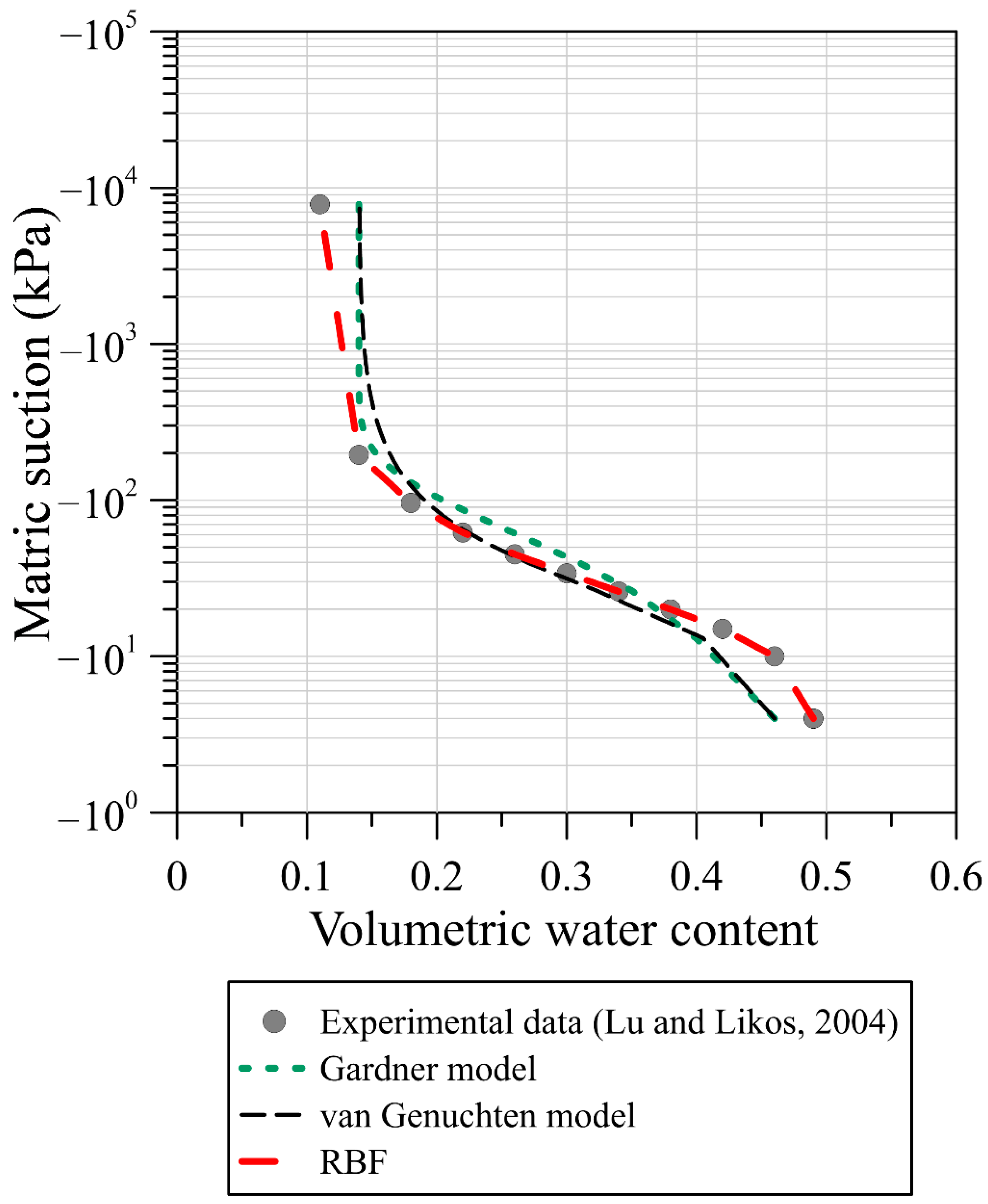
To illustrate the proposed RBF model, we compare the proposed RBF fitting model to several SWCC models, including the Gardner model, van Genuchten model, and experimental data by Lu and Likos [32]. The soil type is glacial till. Best fitted parameters of the above SWCC models were obtained by minimizing the RMSE between experimental and predicted SWCC. The predicted SWCC, along with the testing data, is demonstrated in Figure 1. The fitted parameters and the RMSE are presented in Table 2. We then compare the RMSE of the proposed RBF model and those of the Gardner model and van Genuchten model. From Table 2, the RMSE of the Gardner model and van Genuchten model are only on the order of . The RMSE of the proposed RBF model, however, can reach the order of . It is significant that excellent agreement and highly accurate SWCC achieved by the proposed RBF model can be obtained. From the curve fitting results, we found that the RBF achieves the best estimate for volumetric water content and matric suction to build the representation of the SWCC of glacial till among those SWCC models, as shown in Figure 1.
4. Numerical Methods for Richards Equation
4.1. The RBF Methods for the Richards Equation
With the superior capability of dealing with partial differential equation, the RBF collocation method is one of the prominent methods for solving partial differential equations [33]. We assume that the pressure head can be estimated using the RBF approximation as
where denotes expansion coefficients. The RP RBF depicted in Equation (13) is utilized. The above equation can also be written as
where denotes the interpolation matrix, and . Proposed by Sarra [34], the nth derivative of Equation (17) is then computed as
By the same manner, we have the matrix form as
where . It is often more efficient to use the derivative matrix as
where denotes derivative matrix, and denotes inverse of the A matrix. The spatial derivative of the Equation (17) is then approximated as
The nonlinear Richards equation, as depicted in Equation (6), is then discretized in space and time domains utilizing RBF to acquire the following equation as
Since the above equation is nonlinear, the iteration method is required to obtain the solution of the nonlinear Richards equation. The solution process of the iteration method is described as follows.
4.2. The Fictitious Time Integration Method
For dealing with the nonlinear algebraic equations, as depicted in Equation (23), the iteration methods are mostly applied. An iteration method named the fictitious time integration method (FTIM) was developed by Liu and Atluri [24]. The FTIM tackles the nonlinear Richards equation by introducing a fictitious time. From Equation (7), we may obtain and . It is obvious that and are both functions of the matric potential. In the Gardner model where is used for the fitting from the SWCC. However, can also be obtained directly from the experimental data using the RBF fitting. Accordingly, we may rewrite Equation (23) as follows.
where is the collocation number. The iterative scheme of the FTIM for solving the Richards equation can then be expressed as follows.
where denotes h at the kth discrete time, m denotes a factor ranging from zero to one, denotes fictitious time step size, denotes a fictitious damping coefficient, and denotes fictitious time, defined as . Equation (25) is adopted to solve the system of nonlinear Richards equation resulted from the RBF spatial discretization and Euler temporal discretization.
Beginning by giving an initial guess of the pressure head, we then utilize Equation (25) from to the final elapsed time. The iterative procedure of the FTIM ends while one of the following convergence criteria is achieved.
where , itn denotes number of iterations, denotes convergence criteria, and denotes maximum iterations. In this study, we consider and .
5. Landslide Stability for Unsaturated Soils
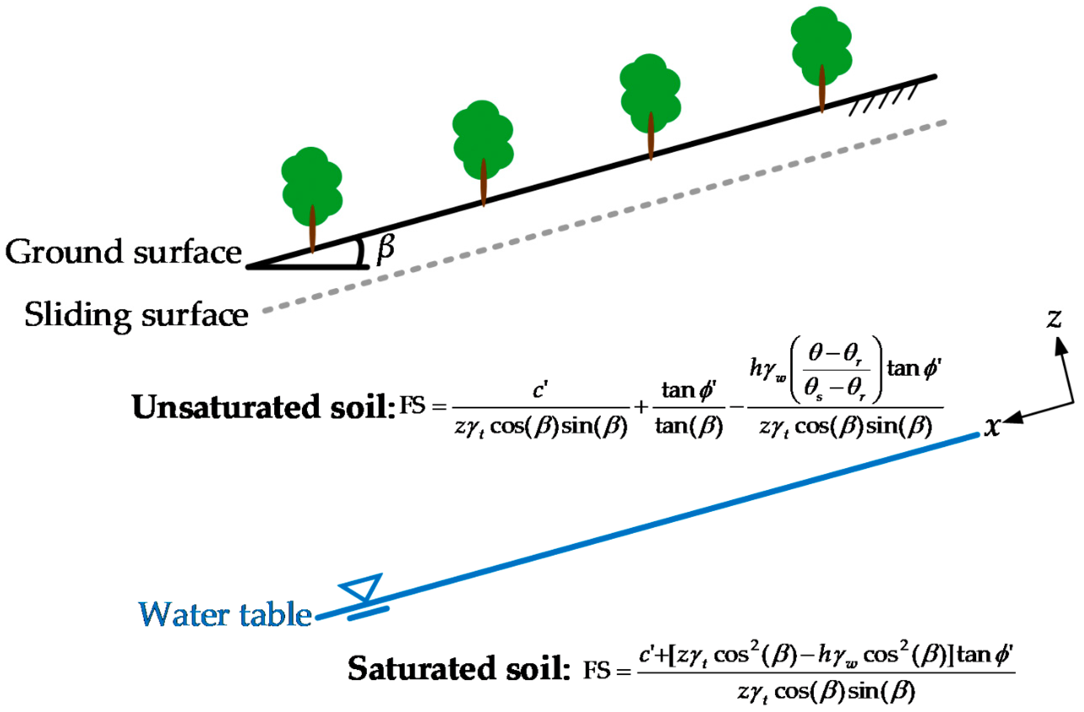
To model the infiltration-induced landslides in unsaturated soils, the landslide stability analysis linked to the RBF approach with the fluctuation of transient pressure head is developed. The infiltration-induced landslides in unsaturated soils is usually very close to the ground surface in which the shallow landslide may occur in the period of heavy rainfall. Accordingly, this study emphasizes on shallow translational landslide considering the infinite slope model for the infiltration in unsaturated soils. The infinite slope model is used to analyze the shallow landslide in which the sliding surface along the failure plane [6]. The safety factor is defined as [7]
where FS denotes safety factor, denotes effective cohesiveness, denotes effective friction angle, z denotes soil thickness, and denote unit weight of water and soil, respectively. Fredlund et al. proposed a linear shear strength equation for the unsaturated soil as follows [26]:
where denotes the shear strength of an unsaturated soil, denotes the net normal stress on the plane of failure at failure, denotes the matric suction of the soil on the plane of failure, and denotes the angle of shearing resistance with respect to matric suction.
According to previous studies [27], results show nonlinear shear strength behavior when experimental test are performed over a wide range of suction. Soils that are resistant to desaturation essentially exhibits a linear shear strength behavior over a relatively large range of soil suction. The above equation can be adopted to describe the shear strength behavior with respect to specified soil suction range. The angle of shearing resistance with respect to soil suction exhibit nonlinear shear strength behavior. Therefore, the relationship between the SWCC and the shear strength has been developed. The shear strength of unsaturated soils at any specified value of suction can be described as [28]
where represents the total stress. The above revised shear strength equation is then substituted into Equation (28) for analyzing infiltration-induced landslides in unsaturated slope [27,35]
Figure 2 illustrates the landslide stability for a variably saturated infinite slope. As demonstrated in Figure 2, Equations (28) and (31) are equations of the safety factor for the saturated and unsaturated slope, respectively. The schematic diagram for modeling infiltration-induced landslides in unsaturated soils is depicted in Figure 3.
6. Numerical Examples
6.1. One-Dimensional Steady-State Infiltration Problem
The one-dimensional steady-state flow in the unsaturated soil is described by the Richards equation as
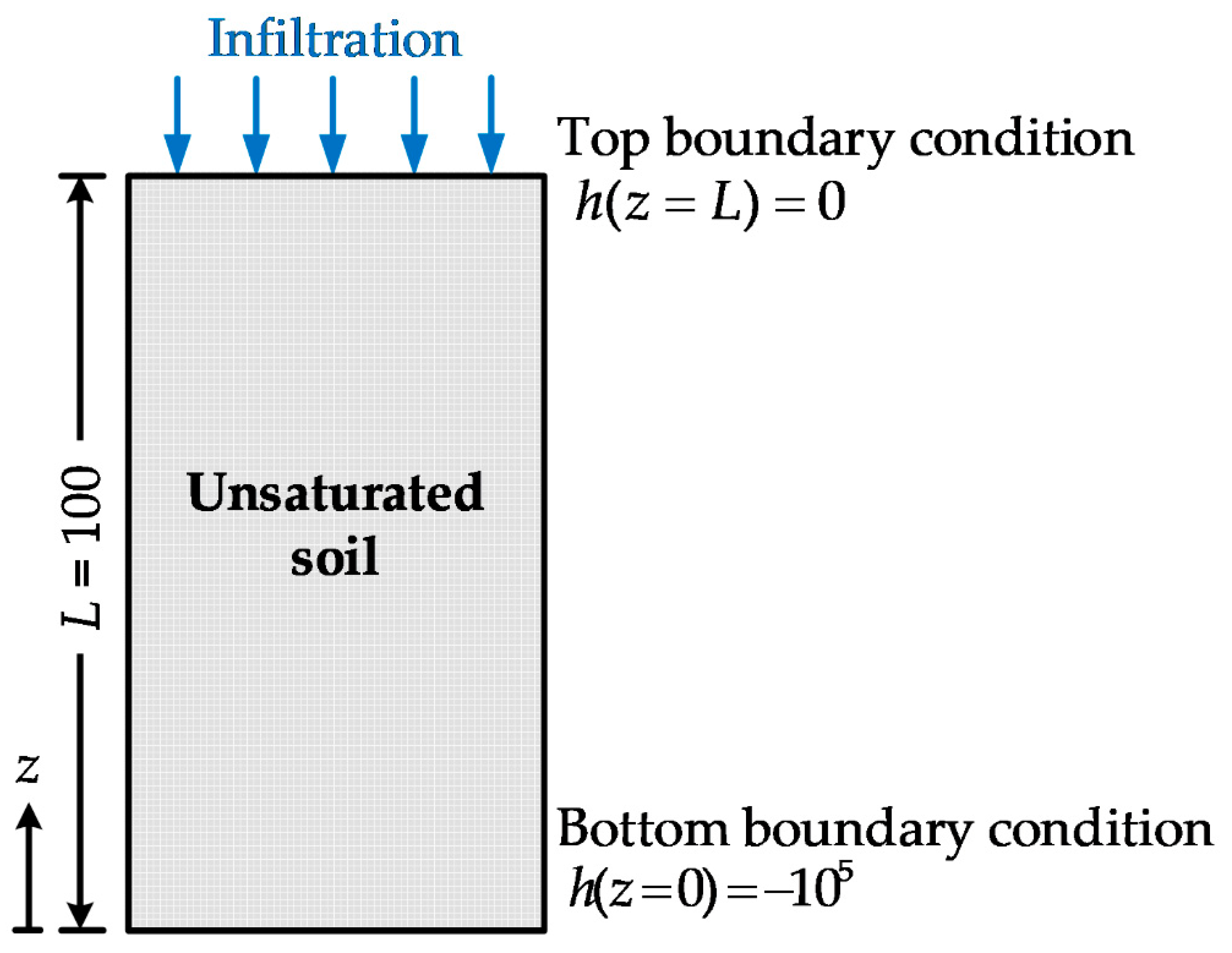
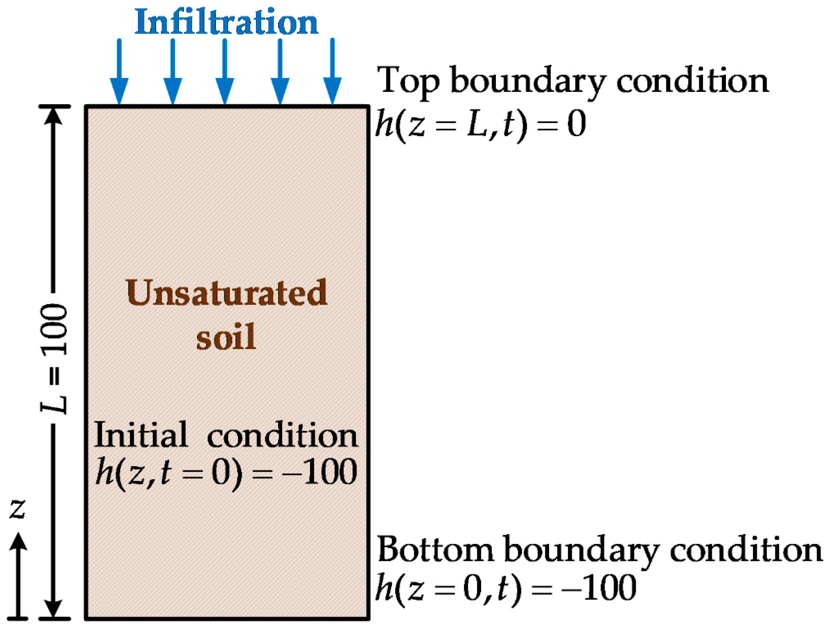
By maintaining the pressure head to be zero, the infiltration is remained at the ground surface, described as
where L is 100 m which is the soil thickness. The boundary condition at the bottom side of the unsaturated soils is in dry condition, defined as follows.
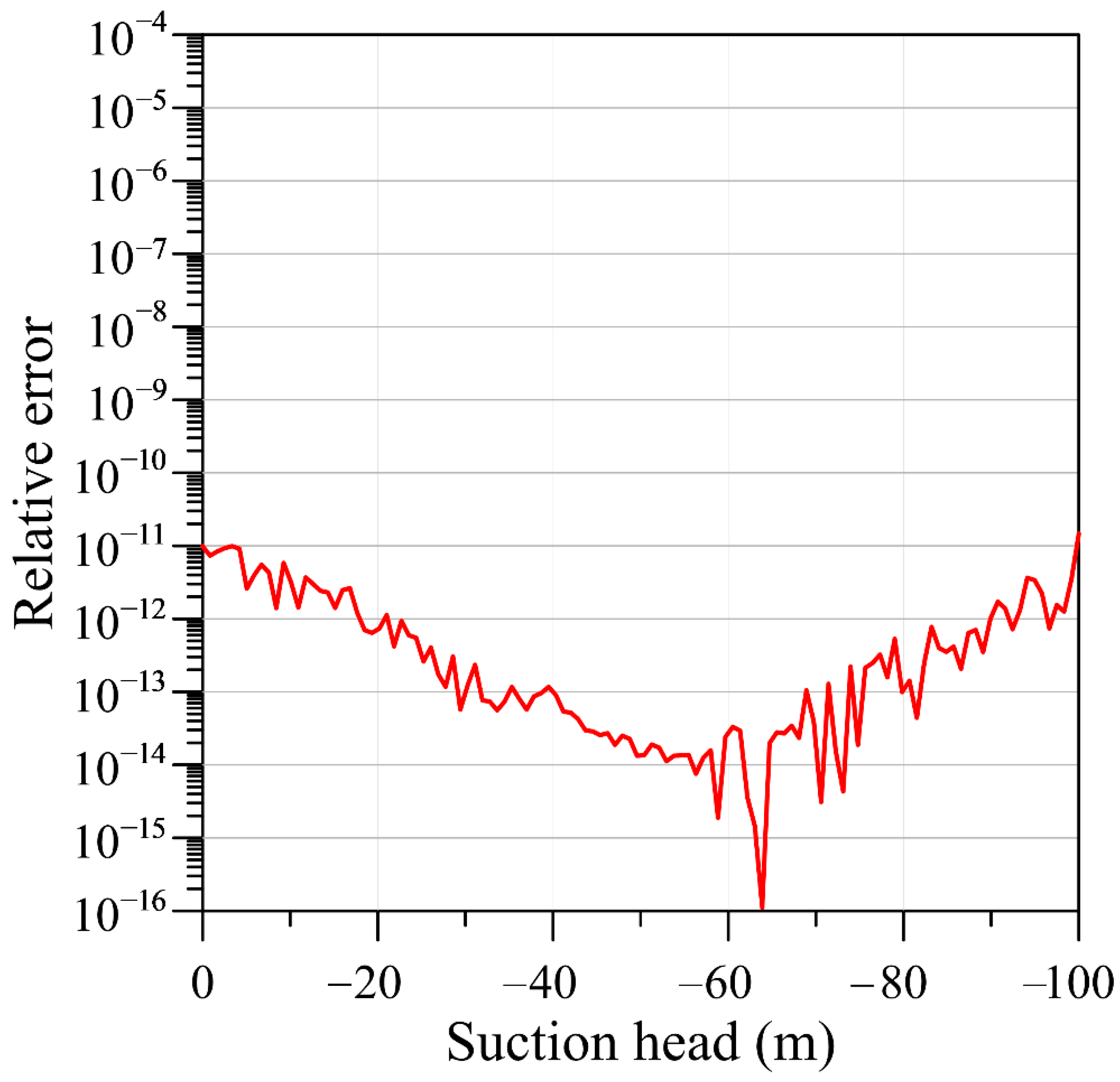
where represents dry pressure head and is m. To describe the nonlinearity of relative hydraulic conductivity, the scattered data produced by the Gardner model are utilized [17]. The type of the unsaturated soils is silty loam, where is . The schematic illustration of one-dimensional steady-state infiltration problem is illustrated in Figure 4.
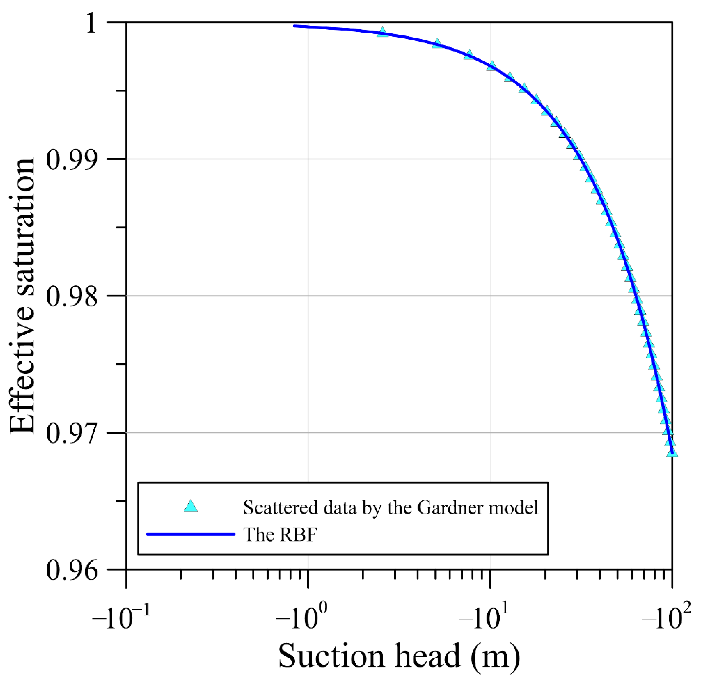
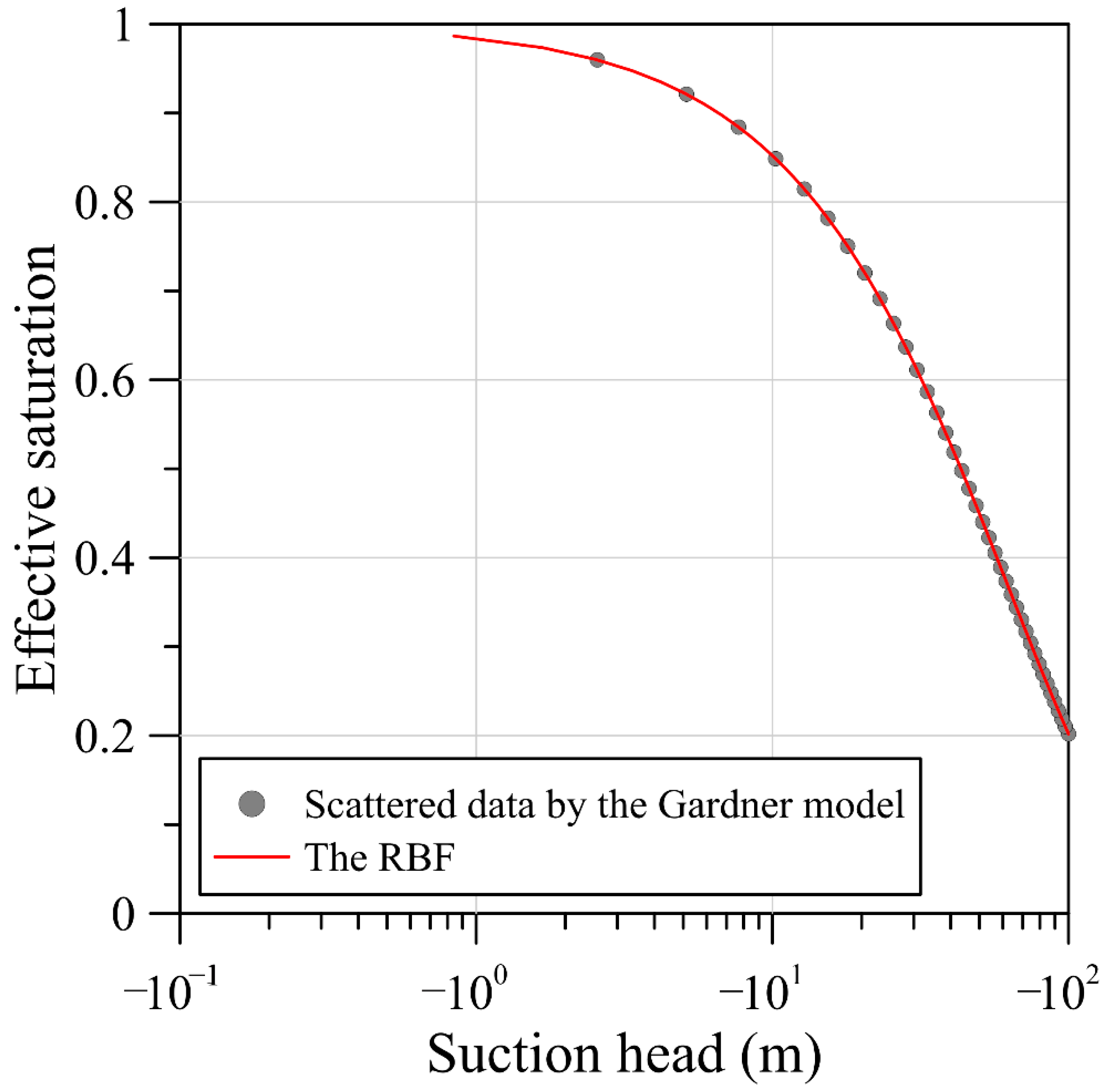
Figure 5 shows the predicted SWCC based on the RBF along with the scattered data by the Gardner model. It is clear that the predicted SWCC based on the RBF closely agrees with the scattered data by the Gardner model. The relative error between the scattered data by the Gardner and RBF model is depicted in Figure 6. The maximum relative error of the predicted SWCC based on the RBF is in the order of . It is significant that excellent agreement is achieved and highly accurate SWCC can be obtained by the RBF.
We then compare the accuracy of the results with the following exact solution [36].
The numerical parameters including , , , , and are considered in this numerical implementation. We considered two boundary points, 34 interior points, and 34 center points. In this example, the SWCC using the RBF, Gardner and van Genuchten model are adopted. The pore size distribution parameter of the Gardner model is . The fitted parameters of the van Genuchten model are and . Figure 7 illustrates the comparison of the computed pressure using the proposed RBF, Gardner, and van Genuchten model with the exact solution. From Figure 7, it is clear that the computed pressure head using the proposed RBF and the Gardner model agree well with the exact solution. However, the computed pressure head using the van Genuchten model may not exactly fit with the exact solution. The main reason is that the above exact solution adopted is basically developed by the Gardner model. This is the reason why excellent agreement is achieved and accurate numerical solutions can be obtained by using the Gardner model. Results obtained shows that the validity of the proposed RBF approach is achieved in the one-dimensional steady-state infiltration problem.
6.2. The Green–Ampt Problem
The second example is the analyzing of the one-dimensional Green–Ampt problem [37], as defined in Equation (6). The initial condition is as
The boundary data are given as follows.
As depicted in Equation (38), the ponding on the ground surface is assigned. The unsaturated soil is in dry condition until the infiltration starts to gradually flow through the unsaturated soil.
The exact solution of the one-dimensional Green–Ampt problem is as [36]
where , , and . The soil thickness is 100 m. The type of the unsaturated soil is sand. To define the nonlinearity of relative hydraulic conductivity, the scattered data produced by the Gardner model are utilized, where , , , m/h, and total time is 0.25 h. The schematic illustration of one-dimensional Green–Ampt problem is illustrated in Figure 8.
The number of the interior points, center points, and boundary points are considered to be 48, 48, and two. The numerical parameters including , , , , , and are adopted. Figure 9 shows the predicted SWCC based on the RBF along with the scattered data by the Gardner model. It is clear that the predicted SWCC based on the RBF closely agrees with the scattered data by the Gardner model. The maximum relative errors of the predicted SWCC based on the RBF is in the order of . It is significant that excellent agreement is achieved and highly accurate SWCC can be obtained by the RBF.
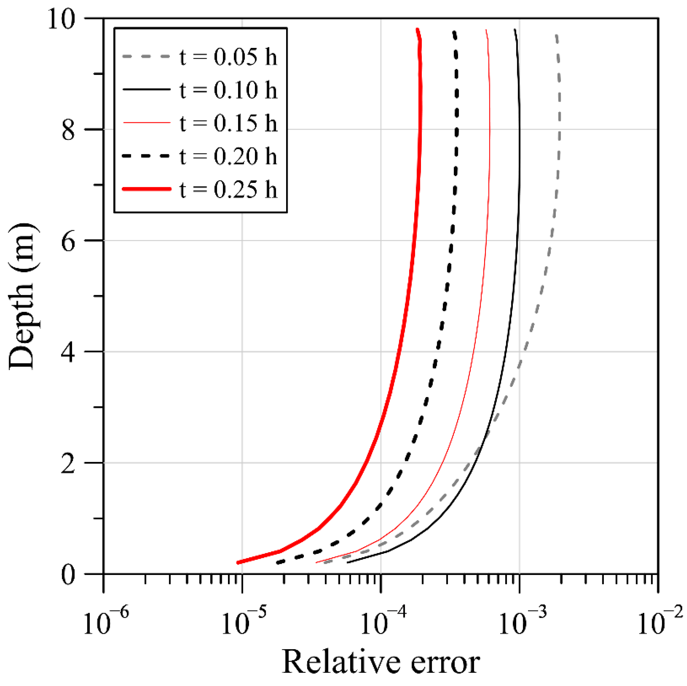
To clearly demonstrate the predicted pressure head, the computed results using the RBF, Gardner and van Genuchten model on different simulation time were compare with the exact solution. The fitted parameters of the van Genuchten model are and . Figure 10 demonstrates the comparison of one-dimensional transient flow in unsaturated soil with the exact solution. It is obvious that the computed pressure head using the proposed RBF and the Gardner model agree well with the exact solution, as depicted in Figure 10. We compare the relative error of the RBF with that of the exact solution, as depicted in Figure 11. The maximum relative error is in the order of to .
6.3. Infiltration-Induced Landslide Problem
The modeling of infiltration-induced landslide in unsaturated soils is presented. The illustration of the unsaturated inclined slope is depicted in Figure 12. We consider the thickness of the unsaturated inclined slope and the slope angle to be 10 m and 35 degrees, respectively. Equation (6) is adopted for this example.
The unsaturated soils are in dry condition until the infiltration starts to gradually flow through the unsaturated soil. The initial and boundary conditions are assigned as follows.
To depict the nonlinearity of unsaturated soils, the experimental data are utilized [32]. The soil type is sandy soil. The parameter of pore size distribution is , the saturated water content is 0.50, the residual water content is 0.11, the saturated hydraulic conductivity is 1 m/h, the effective cohesiveness is 4.6 kPa, the effective friction angle is 30 degrees, the soil unit weight is 21.5 kN/m3, and total simulation time is 0.1 h. The fitted parameters of the van Genuchten model are and . There are 48 interior points, 48 center points, and two boundary points. The numerical parameters including , , , , , and are utilized.
Figure 13 shows the predicted SWCCs using the RBF fitting model, the Gardner model and the van Genuchten model comparing with the experimental data. It is significant that the predicted SWCC using the proposed RBF fitting model presents the best fitting with the MAE in the order of among those empirical Gardner model and van Genuchten model. We then evaluate the computed matric potential using the Gardner model, van Genuchten model, and the proposed RBF. Figure 14 demonstrates a plot of matric potential versus depth at different simulation time. From Figure 14, it is found that the matric potential obtained by the Gardner model, van Genuchten model, and the proposed RBF are different. The conventional Gardner and van Genuchten models have simple forms considering only one and three fitting parameters, respectively. Accordingly, these SWCC models may be only applicable for fitting the SWCC of certain soil textures. However, the advantage of the proposed RBF model lies in its applicability in fitting almost any soil types due to the fact that many weighting coefficients can be utilized in the RBF model for approximating the high nonlinearity of the SWCC. It appears that the matric potential obtained by the proposed RBF may depict the physical property of unsaturated soils.
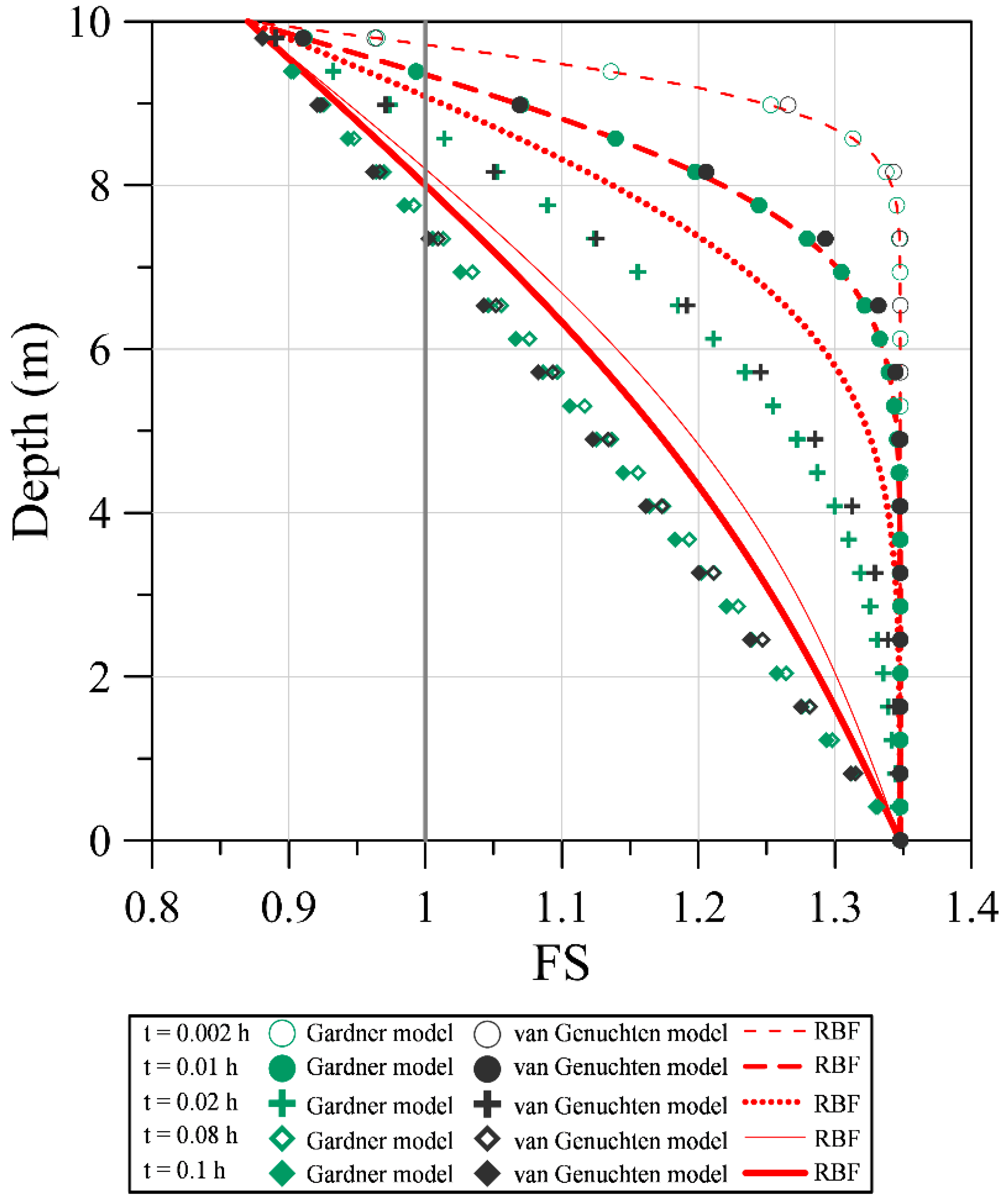
To analyze the infiltration-induced landslides in unsaturated soils, the hydrological model considering the stability analysis of infinite slope is then carried out. To evaluate the safety factor for the unsaturated slope, Equations (28) and (31) are utilized. Figure 15 depicts the computed results of safety factor. As illustrated in Figure 15, we also found that the computed FS obtained by different methods are very different because Gardner or van Genuchten models may have limitations to fit the SWCC. Since excellent agreement and highly accurate SWCC using the proposed RBF model can be yielded (as depicted in Figure 13), the FS obtained by the proposed RBF may comprehensively consider the physical property of unsaturated soils. Furthermore, the FS obtained by the proposed RBF demonstrates that landslide would be triggered rapidly when FS is less than 1.0 and the lowest FS may occur at the z = 8 to 10 m during the infiltration, as shown in Figure 15. From Figure 14 and Figure 15, it is found that the slope stability is highly related to the fluctuation of matric potential in unsaturated soils during the infiltration process.
7. Conclusions
A novel RBF approach for infiltration-induced landslides in unsaturated soils is presented. The study emphasizes on the importance of infiltration processes to predict landslide hazard. Significant findings are concluded as follows:
- (1)
- This article is a leading attempt to model infiltration-induced landslides in unsaturated soils utilizing the RBF method. Since the soil water characteristic curve is a primary factor defining the nonlinearity of unsaturated soils, we first utilize the RBF for curve fitting to build the representation of the SWCC. Results demonstrate that the RBF seems to be advantageous for reconstructing the SWCC of glacial till and sand soil with better estimation of the relationship than conventional parametric Gardner and van Genuchten models.
- (2)
- For solving the nonlinear Richards equation, we developed a novel work using the RBF approach with the infiltration boundary conditions. The fictitious time integration method is adopted in the RBF approach for tackling the nonlinearity of the Richards equation. We propose the novel RBF approach for reconstructing the SWCC to directly solving the nonlinear Richards equation such that the conventional parametric Gardner model and van Genuchten model are not required in the proposed approach.
- (3)
- The hydrological model considering the stability analysis of infinite slope is conducted to analyze the infiltration-induced landslides with emphasis on the behavior of unsaturated soils. Additionally, the proposed RBF method for the nonlinear Richards equation in an inclined slope can be widely applied for disparate types of unsaturated soils. We also found that the stability of landslides is highly related to the variation of matric potential in unsaturated soils during the infiltration process.
Author Contributions
Designing the study, C.-Y.K.; performing the analysis, C.-Y.L.; formulation, C.-Y.K. and C.-Y.L.; writing and editing, C.-Y.K., C.-Y.L. and F.T.-C.T. All authors have read and agreed to the published version of the manuscript.
Funding
No external funding is received.
Institutional Review Board Statement
Not applicable.
Informed Consent Statement
Not applicable.
Data Availability Statement
Research data are available on request.
Conflicts of Interest
The authors declare no conflict of interest.
References
- Chiang, S.H.; Chang, K.T. The potential impact of climate change on typhoon-triggered landslides in Taiwan, 2010–2099. Geomorphology 2011, 133, 143–151. [Google Scholar] [CrossRef]
- Mani, A.; Tsai, F.; Kao, S.C.; Naz, B.S.; Ashfaq, M.; Rastogi, D. Conjunctive management of surface and groundwater resources under projected future climate change scenarios. J. Hydrol. 2016, 540, 397–411. [Google Scholar] [CrossRef] [Green Version]
- Bordoni, M.; Galanti, Y.; Bartelletti, C.; Persichillo, M.G.; Barsanti, M.; Giannecchini, R.; D’Amato Avanzi, G.; Cevasco, A.; Brandolini, P.; Galve, J.P.; et al. The influence of the inventory on the determination of the rainfall-induced shallow landslides susceptibility using generalized additive models. Catena 2020, 193, 104630. [Google Scholar] [CrossRef]
- Wu, L.Z.; Selvadurai, A.P.S.; Zhang, L.M.; Huang, R.Q.; Huang, J. Poro-mechanical coupling influences on potential for rainfall-induced shallow landslides in unsaturated soils. Adv. Water Resour. 2016, 98, 114–121. [Google Scholar] [CrossRef]
- Fusco, F.; De Vita, P.; Mirus, B.B.; Baum, R.L.; Allocca, V.; Tufano, R.; Calcaterra, D. Physically based estimation of rainfall thresholds triggering shallow landslides in volcanic slopes of Southern Italy. Water 2019, 11, 1915. [Google Scholar] [CrossRef] [Green Version]
- Zhang, L.L.; Fredlund, M.D.; Fredlund, D.G.; Lu, H.; Wilson, G.W. The influence of the unsaturated soil zone on 2-D and 3-D slope stability analyses. Eng. Geol. 2015, 193, 374–383. [Google Scholar] [CrossRef]
- Lu, N.; Godt, J. Infinite slope stability under steady unsaturated seepage conditions. Water Resour. Res. 2008, 44, 1–13. [Google Scholar] [CrossRef]
- Keles, F.; Nefeslioglu, H.A. Infinite slope stability model and steady-state hydrology-based shallow landslide susceptibility evaluations: The Guneysu catchment area (Rize, Turkey). Catena 2021, 200, 105161. [Google Scholar] [CrossRef]
- Urciuoli, G.; Pirone, M.; Picarelli, L. Considerations on the mechanics of failure of the infinite slope. Comput. Geotech. 2019, 107, 68–79. [Google Scholar] [CrossRef]
- Iverson, R.M. Landslide triggering by rain infiltration. Water Resour. Res. 2000, 36, 1897–1910. [Google Scholar] [CrossRef] [Green Version]
- Baum, R.L.; Savage, W.Z.; Godt, J.W. TRIGRS—A Fortran program for transient rainfall infiltration and grid-based regional slope-stability analysis. US Geol. Surv. Open-File Rep. 2002, 424, 38. [Google Scholar]
- Ciurleo, M.; Mandaglio, M.C.; Moraci, N. Landslide susceptibility assessment by TRIGRS in a frequently affected shallow instability area. Landslides 2019, 16, 175–188. [Google Scholar] [CrossRef]
- Liu, W.; Luo, X.; Huang, F.; Fu, M. Uncertainty of the soil–water characteristic curve and its effects on slope seepage and stability analysis under conditions of rainfall using the markov chain monte carlo method. Water 2017, 9, 758. [Google Scholar] [CrossRef] [Green Version]
- Rajesh, S.; Roy, S.; Madhav, S. Study of measured and fitted SWCC accounting the irregularity in the measured dataset. Int. J. Geotech. Eng. 2017, 11, 321–331. [Google Scholar] [CrossRef]
- Chiu, C.F.; Yan, W.M.; Yuen, K.V. Reliability analysis of soil–water characteristics curve and its application to slope stability analysis. Eng. Geol. 2012, 135, 83–91. [Google Scholar] [CrossRef]
- Šimůnek, J.; Jarvis, N.J.; Van Genuchten, M.T.; Gärdenäs, A. Review and comparison of models for describing non-equilibrium and preferential flow and transport in the vadose zone. J. Hydrol. 2003, 272, 14–35. [Google Scholar] [CrossRef]
- Gardner, W.R. Some steady-state solutions of the unsaturated moisture flow equation with application to evaporation from a water table. Soil Sci. 1958, 85, 228–232. [Google Scholar] [CrossRef]
- van Genuchten, M.T. A closed-form equation for predicting the hydraulic conductivity of unsaturated soils. Soil Sci. Soc. Am. J. 1980, 44, 892–898. [Google Scholar] [CrossRef] [Green Version]
- Fredlund, D.G.; Xing, A. Equations for the soil-water characteristic curve. Can. Geotech. J. 1994, 31, 521–532. [Google Scholar] [CrossRef]
- Celia, M.A.; Bouloutas, E.T.; Zarba, R.L. A general mass-conservative numerical solution for the unsaturated flow equation. Water Resour. Res. 1990, 26, 1483–1496. [Google Scholar] [CrossRef]
- Liu, C.Y.; Ku, C.Y.; Huang, C.C.; Lin, D.G.; Yeih, W.C. Numerical solutions for groundwater flow in unsaturated layered soil with extreme physical property contrasts. Int. J. Nonlinear Sci. Numer. Simul. 2015, 16, 325–335. [Google Scholar] [CrossRef]
- List, F.; Radu, F.A. A study on iterative methods for solving Richards’ equation. Comput. Geosci. 2016, 20, 341–353. [Google Scholar] [CrossRef] [Green Version]
- Hardy, R.L. Multiquadric equations of topography and other irregular surfaces. J. Geophys. Res. 1971, 76, 1905–1915. [Google Scholar] [CrossRef]
- Liu, C.S.; El-Zahar, E.R.; Chang, C.W. A boundary shape function iterative method for solving nonlinear singular boundary value problems. Math. Comput. Simul. 2021, 187, 614–629. [Google Scholar] [CrossRef]
- Qi, S.; Vanapalli, S.K. Influence of swelling behavior on the stability of an infinite unsaturated expansive soil slope. Comput. Geotech. 2016, 76, 154–169. [Google Scholar] [CrossRef]
- Fredlund, D.G.; Morgenstern, N.R.; Widger, R.A. The shear strength of unsaturated soils. Can. Geotech. J. 1978, 15, 313–321. [Google Scholar] [CrossRef]
- Vanapalli, S.K.; Fredlund, D.G.; Pufahl, D.E.; Clifton, A.W. Model for the prediction of shear strength with respect to soil suction. Can. Geotech. J. 1996, 33, 379–392. [Google Scholar] [CrossRef]
- Fredlund, D.G.; Morgenstern, N.R. Stress state variables for unsaturated soils. J. Geotech. Eng.-Asce 1977, 103, 447–466. [Google Scholar] [CrossRef]
- Mualem, Y. A new model for predicting the hydraulic conductivity of unsaturated porous media. Water Resour. Res. 1976, 12, 513–522. [Google Scholar] [CrossRef] [Green Version]
- Baiamonte, G. Analytical solution of the Richards equation under gravity-driven infiltration and constant rainfall intensity. J. Hydrol. Eng. 2020, 25, 04020031. [Google Scholar] [CrossRef]
- Ku, C.Y.; Hong, L.D.; Liu, C.Y.; Xiao, J.E. Space–time polyharmonic radial polynomial basis functions for modeling saturated and unsaturated flows. Eng. Comput. 2021, 1–14. [Google Scholar] [CrossRef]
- Lu, N.; Likos, W.J. Rate of capillary rise in soil. J. Geotech. Geoenviron. Eng. 2004, 130, 646–650. [Google Scholar] [CrossRef]
- Kansa, E.J. Multiquadrics—A scattered data approximation scheme with applications to computational fluid-dynamics—II solutions to parabolic, hyperbolic and elliptic partial differential equations. Comput. Math. Appl. 1990, 19, 147–161. [Google Scholar] [CrossRef] [Green Version]
- Sarra, S.A. Adaptive radial basis function methods for time dependent partial differential equations. Appl. Numer. Math. 2005, 54, 79–94. [Google Scholar] [CrossRef] [Green Version]
- Ku, C.Y.; Liu, C.Y.; Su, Y.; Xiao, J.E. Modeling of transient flow in unsaturated geomaterials for rainfall-induced landslides using a novel spacetime collocation method. Geofluids 2018, 2018, 7892789. [Google Scholar] [CrossRef] [Green Version]
- Tracy, F.T. Clean two- and three-dimensional analytical solutions of Richards’ equation for testing numerical solvers. Water Resour. Res. 2006, 42, 8. [Google Scholar] [CrossRef]
- Green, W.H.; Ampt, G.A. Studies on soil physics I. The flow of air and water through soils. J. Agric. Sci. 1911, 4, 1–24. [Google Scholar]
Figure 1.
The fitted results of the SWCC.

Figure 2.
Landslide stability for a variably saturated infinite slope.

Figure 3.
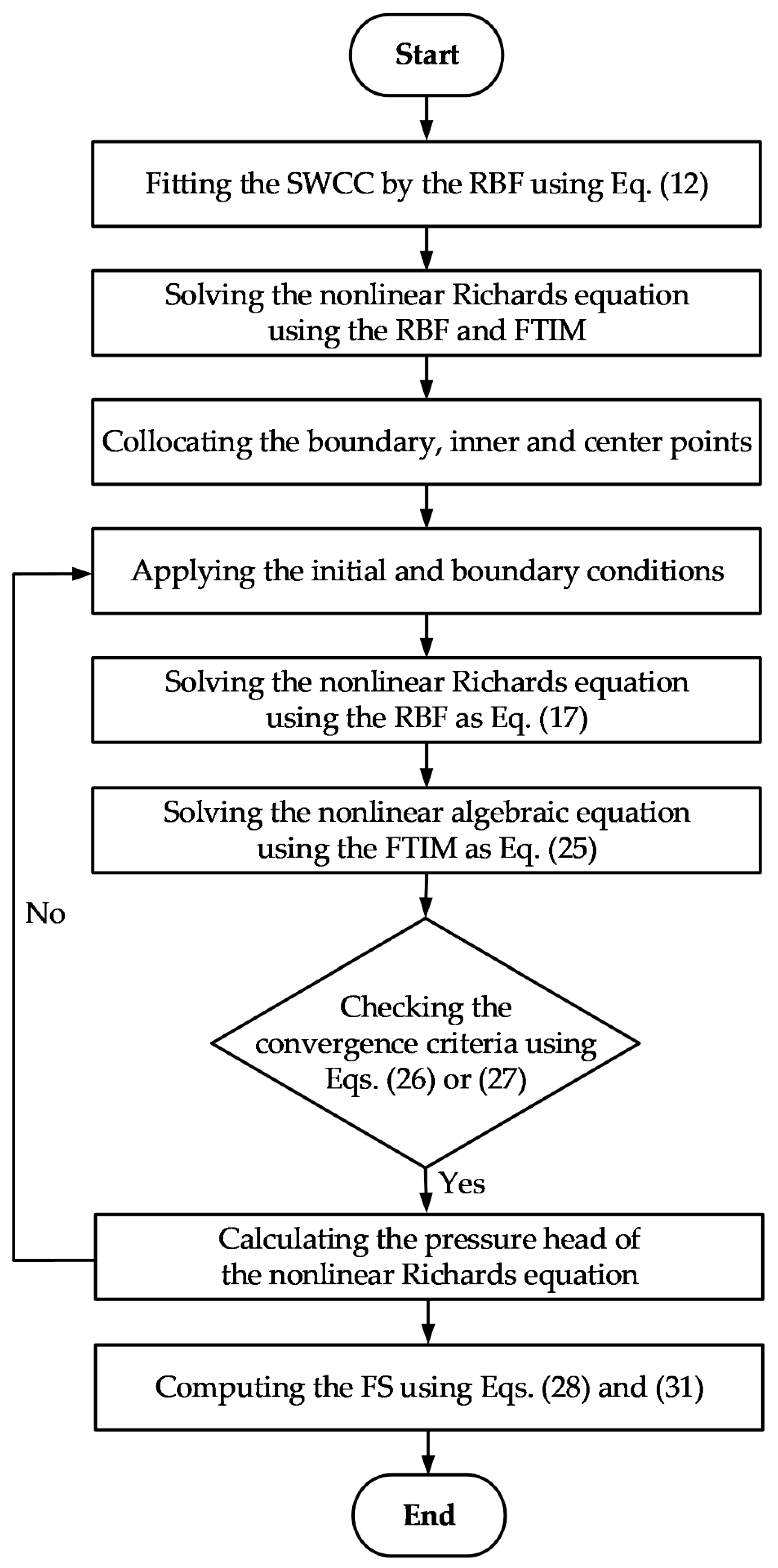
The flowchart of this study.

Figure 4.
Schematic illustration of one-dimensional steady-state infiltration problem.

Figure 5.
Comparing effective saturation using RBF with scattered data by the Gardner model.

Figure 6.
The relative error between the scattered data by the Gardner model and the RBF.

Figure 7.
Comparison of the pressure head with the exact solution.

Figure 8.
A schematic of one-dimensional Green–Ampt problem.

Figure 9.
Comparing effective saturation using RBF with scattered data by the Gardner model.

Figure 10.
Comparison with the exact solutions.

Figure 11.
Relative error of the computed results using the RBF.

Figure 12.
Illustration of unsaturated inclined slope.

Figure 13.
The fitted results of the SWCC (sandy soil).

Figure 14.
Computed matric potential.

Figure 15.
Computed FS.


Table 1.
Types of RBF.
| Type of RBF | RBF |
|---|---|
| Gaussian | |
| Multiquadric | |
| Inverse quadratic | |
| Inverse multiquadric | |
| Polyharmonic spline | |
| Thin plate spline | |
| Radial polynomials |
Notation: c denotes shape parameter.
Table 2.
The fitted parameters and RMSE in the example.
| SWCC Model | Fitted Parameters | RMSE |
|---|---|---|
| Gardner model | ||
| van Genuchten model | ||
| RBF |
Publisher’s Note: MDPI stays neutral with regard to jurisdictional claims in published maps and institutional affiliations. |
© 2022 by the authors. Licensee MDPI, Basel, Switzerland. This article is an open access article distributed under the terms and conditions of the Creative Commons Attribution (CC BY) license (https://creativecommons.org/licenses/by/4.0/).
Share and Cite
MDPI and ACS Style
Ku, C.-Y.; Liu, C.-Y.; Tsai, F.T.-C. A Novel Radial Basis Function Approach for Infiltration-Induced Landslides in Unsaturated Soils. Water 2022, 14, 1036. https://doi.org/10.3390/w14071036
AMA Style
Ku C-Y, Liu C-Y, Tsai FT-C. A Novel Radial Basis Function Approach for Infiltration-Induced Landslides in Unsaturated Soils. Water. 2022; 14(7):1036. https://doi.org/10.3390/w14071036
Chicago/Turabian StyleKu, Cheng-Yu, Chih-Yu Liu, and Frank T.-C. Tsai. 2022. "A Novel Radial Basis Function Approach for Infiltration-Induced Landslides in Unsaturated Soils" Water 14, no. 7: 1036. https://doi.org/10.3390/w14071036
Note that from the first issue of 2016, this journal uses article numbers instead of page numbers. See further details here.