Article

Water Procurement Time and Its Implications for Household Water Demand—Insights from a Water Diary Study in Five Informal Settlements of Pune, India

1
Department of Economics, Helmholtz Centre for Environmental Research—UFZ, Permoser Str. 15, 04318 Leipzig, Germany
2
Faculty of Economics and Business Management, Institute of Infrastructure and Resources Management, Leipzig University, Grimmaische Str. 12, 04109 Leipzig, Germany
*
Author to whom correspondence should be addressed.
Water 2022, 14(7), 1009; https://doi.org/10.3390/w14071009
Submission received: 4 February 2022 / Revised: 7 March 2022 / Accepted: 18 March 2022 / Published: 22 March 2022
(This article belongs to the Section Water Use and Scarcity)

Abstract

:
Many private households spend considerable amounts of time accessing water, for instance by walking to and queuing at public access points, or by filling storage vessels at taps with low flow rates. This time has an opportunity cost, which can be substantial and may impact which water services and quantities of water households demand. In a novel form of diary study, we gathered detailed water consumption and time use data from 50 households in five informal settlements of the Indian metropolis Pune, accompanied by a household survey and in-depth interviews. With the data, we characterize water collection behaviors and assign monetary values to water procurement time. We statistically analyze the effects of time cost on consumed quantities in several two-level mixed-effect models. Household members in our sample spend up to several hours each day filling storage vessels, even if a private connection to the piped network is available. Average time cost amounted to the equivalent of 4.23–13.81% of monthly household cash income. Our analyses indicate that procurement time reduces quantitative water demand in a significant way. The households incurring the highest per-unit time cost consumed water quantities below minimum levels recommended for human health. This substantiates that time costs can impede access to water and are a relevant issue for water management and policy.

1. Introduction

In recent decades, a key focus of water supply planning and management has been the expansion of water supply infrastructures to increase access to water, which has been recognized as a human right by the UN General Assembly [1]. Concurrently, the monitoring of the access-related targets of the Millennium and Sustainable Development Goals registered a steady improvement of access to water, operationalized for instance as the presence of ‘safely managed’ drinking water sources on households’ premises in target 6.1 of the Agenda 2030 [2]. Notwithstanding the fact that considerable accomplishments have been made, it has been pointed out that access is not a binary, but a gradual issue [3] and that the available assessment systems can fail to capture the complexities of the topic [4,5,6]. The literature on the right to water has established that access to water is not merely determined by infrastructures or delivered quantities of water, but by the affordability and the service level or service quality of available water supplies [7,8]. The quality or level of service refers to the most important dimensions shaping access to water, namely the quality and acceptability of supplied water quantities, their spatial accessibility, and their temporal availability [9]. Empirical evidence from many urban and rural areas attests to the importance of considering these dimensions of access. It is estimated that more than one billion people receive intermittent network supply [10] and deal with low temporal availability through a variety of strategies, including self-storage of water or self-supply through private wells [11]. Others purchase market water services in addition to or absence of piped supply [5,12], for example from tanker trucks [13,14], while those with the lowest income frequently walk to public access points, queue there, and carry water home [11,15]. Due to quality concerns, it is also a common practice of private households to use water filters or boil water quantities before drinking or cooking [16,17]. For these activities, households frequently use substantial amounts of their time [18], which is a scarce resource with an opportunity cost [19]. Thus far, this cost is not sufficiently considered in efforts to monitor access to water, even though it may result in “major concern” [5] (p. 365) and “hidden affordability problems” [20] (05019006-1) for the affected households. Despite increasing evidence that time cost of access can create water indigence and vulnerability unobserved by national surveys or commonly used indicators for SDG 6.1 and the human right to water, they have not received appropriate attention from water research, management, and policy.
The conceptualization of cost related to access should therefore be expanded to encompass both pecuniary and non-pecuniary expenditures directed at obtaining water quantities [21]. Besides the network tariff or prices charged by water vendors, pecuniary expenses include, for example, capital investments such as storage equipment or water filtering systems. When household time and physical effort are used for waiting, storing, or hauling water quantities from a remote access point, on the other hand, non-pecuniary costs are incurred. Both types of expenditure are usually aimed at substituting or complementing the services of a supplier [21,22]. It thus can be argued that households (co-)produce water services [21]. How much household production [19]—and thus expenditures of money and time—is necessary, strongly depends on the service level of available options to access water. Research that aims to better understand these complexities is presented with numerous challenges because the non-pecuniary cost of access in general and time cost, in particular, are difficult to ascertain, typically not covered by standard household surveys, and may vary considerably between seasons or with the short-term fluctuations of supply [23]. Existing evidence from areas with low service levels of supply suggests that households, and particularly their female members, use substantial amounts of time each day to obtain water: UNICEF [24] estimates that 200 million hours are spent every day by women and girls collecting water.
With dimensions of this kind, it is reasonable to assume that the opportunity cost of time associated with procuring water will affect which water services [25,26] and which quantities of water are demanded [21]. While the water demand literature reviewed for this paper to some extent accounts for time costs in source choice models [27,28], merely a few studies [29,30,31] have considered the cost of time for “water hauling” explicitly in their estimation of demand for water quantities. These studies estimated demand functions with the predictor “total cost” (i.e., monetary and time cost combined) and found a significant effect on the probability of selecting a specific water source and on quantitative demand. Another strand of economic research addresses time cost by investigating coping cost or averting the cost of ‘unreliable supply’ [32,33,34,35,36]. These studies follow the premise that household expenditures of money and time to obtain drinking water are acts of averting damage, e.g., for human health. Such expenditures can be made ex-ante, for example by purchasing a water filter, or ex-post, e.g., by bearing the cost of treatment for water-borne diseases [16]. Assuming that coping costs reveal household preferences, these approaches then attempt to estimate the monetary value of averting behavior to derive a lower-bound on willingness-to-pay for improved water services (for a more detailed description of this approach see [32]). Depending on the focus of the study, the considered cost items range from expenditure on market water services and durable goods, to the energy cost of pumping or boiling water, to the cost of sick days caused by water-related diseases. Household time dedicated to traveling and waiting at remote water access points has been included as a cost item in a small number of such studies up to date [16,32,33,36,37]. The results indicate that travel costs can be substantial: In their study in rural India, Pattanayak et al. [38] found that more than half of coping costs were traveling costs, while Cook et al. (2016) obtained similar results for households without piped network supply in rural Kenya. Amit and Sasidharan [36] found that traveling costs can amount to up to 22% of coping costs for a household without piped connections in low-income areas in Chennai, India. Whether households may incur time costs even if they have a water connection within their residence, for example when filling storage vessels under low water pressure, has not been investigated by any of the studies reviewed for this article.
The outlined contributions are valuable empirical testimonies to the complexities shaping access to water and the wide array of costs that households may face when procuring water quantities. In this paper, we take inspiration from this previous research but approach the topic with a somewhat different objective:
  • We carry out an analysis focused in-depth and exclusively on the time cost of water procurement for urban households who are supplied at low service levels, both with and without network connections. We refer to time cost as the opportunity cost of the time used for the entire set of activities directed at making water quantities available for usage, including walking, waiting, and the filling of storage vessels. In contrast to parts of the coping cost literature, we include water quantities for both drinking and non-drinking purposes in our analysis. We also call an implicit assumption in most studies dealing with time cost into question, namely that households with an in-house piped network connection do not incur time expenditure [16,30,33]. We approach the analysis with a mixture of qualitative and quantitative, longitudinal data, which has to our knowledge not been attempted in this form. By doing so, we are able to quantify time cost and water consumption more precisely than through standard survey approaches [39,40] and can analyze the dynamics and fluctuations of access conditions over time through repeated measurements for the same households.
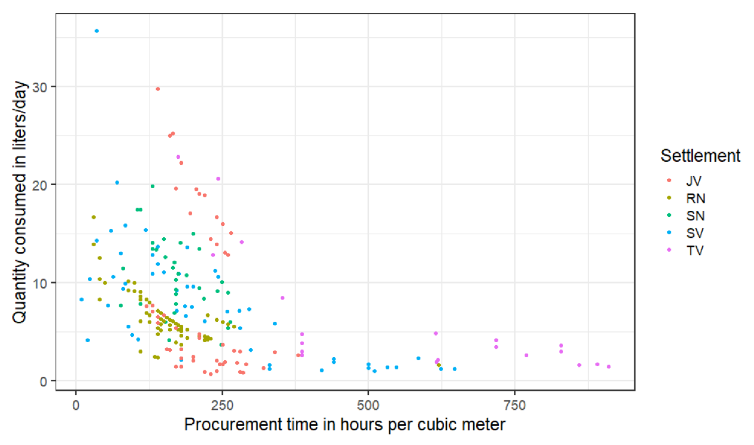
  • We use the quantitative data to assign monetary values to time expenditure based on wage rates and empirically investigate the impacts of water procurement time on consumption decisions. As we have argued in-depth in another article [21], the opportunity cost of water procurement time should affect which water services and which quantities of water households demand. We statistically analyze data on time expenditure and water consumption to test whether we find evidence that (1) time cost negatively impacts consumed quantities and (2) this correlation is more pronounced for those with a higher opportunity cost of time.
To carry out these objectives, we analyze high-resolution water consumption and time use data [41] collected through mixed field methods, in particular, a water diary experiment, a household survey, and in-depth qualitative interviews. In the course of the diary study, we asked 50 households from five so-called “slums” in the Indian metropolis Pune to document their water-related activities in high detail for one week, resulting in disaggregated data on supply fluctuations, household consumption of water quantities by source and the usage of time to collect them. In order to focus on the economic effects of time cost on demanded quantities, we selected areas where piped network services are provided free of monetary charges, albeit with strong differences in service levels. The five settlements reflect heterogeneous water supply conditions, at times even within a radius of one hundred meters. The results demonstrate that many households incur substantial time costs, measured both in daily procurement time and in monetary terms as a fraction of their cash income or time endowment. The economic analysis substantiates that consumption decisions are likely to be impacted by time cost to a significant extent. Most households from the “expensive” end of the time cost spectrum consumed quantities below minimum levels recommended in the literature [42].
The remainder of this paper is structured as follows. The next section briefly discusses how the economic literature usually assigns a monetary value to household time and which impact time cost may be expected to have on consumption decisions, following household production theory. The third section describes the design of our mixed field methods approach, in particular, the water diary experiment. Section 4 presents demographic and socioeconomic profiles of the households participating in the study, as well as descriptions of their water supply situation and water procurement time. In Section 5, we present the economic valuation of time cost and the results of several statistical models of the impact of water procurement time on consumed quantities. Section 6 discusses the relevance and limitations of our findings, Section 7 concludes.

2. Water Procurement Time: Economic Value and Implications for Household Demand for Water Services

2.1. Assigning Economic Value to Water Procurement Time

Household activities associated with collecting, storing, and treating water quantities can be considered unpaid or non-market work by standard definitions from the economic literature [43]. A widely used approach of distinguishing unpaid work from personal (or leisure) time is the so-called third-person criterion, first proposed by Margaret Reid [44], which postulates that in case someone else could be paid to carry out a specific activity, it should have economic value. This is certainly the case for collecting water from a remote source but also for activities within the household, such as filling storage vessels or boiling water before drinking it. To ascertain the economic value of such an activity and the household time invested into it is—in absence of a market transaction—not straightforward. The economic literature has identified a variety of methodological approaches to assign a monetary value to unpaid work. The approaches could loosely be divided into three groups, namely wage-based [45], output-based [46], and stated-preference-based approaches [47].
Wage-based methods assume that the value of a productive household activity can be “borrowed from the market” [46] (p. 128) in the sense that specific wage rates, i.e., market valuations for household labor factor inputs, accurately capture the value of unpaid work time. Applications of wage-based methods differ with regard to the choice of wage rate, which could be (i) the household members’ individual wage rates because “otherwise the homemaker would choose to enter the labor market” [48] (p. 216) or (ii) the shadow price of a close market substitute, for example, the wage rate charged for the services of domestic help. Output-based methods do not value individual units of time but rather seek to approximate the value of the product of household activities, by establishing the price of a similar good or service on the market and subtracting the prices of inputs. Thus, the focus is on the value-added [46] through household time which addresses a criticism pointed at wage-based methods, namely that there is no clear relationship between wage rates and the output that individuals with different capabilities can produce in one hour [49,50]. Finally, stated-preferences-approaches seek to establish the value of unpaid work time through subjective valuations by implementing, for instance, contingent valuation experiments with households (for more information see the overview by [47]).
The applicability of methods seems to be determined by the purpose of the valuation [45]. If the purpose is to derive a meaningful and comparative valuation of the goods and services produced by the households, the output method seems advantageous. If, on the other hand, the purpose of the analysis is to understand cost from the perspective of an individual, an approach based on wages reflecting opportunity cost seems more consistent with economic theory [19]. Wage-based approaches have been used in the majority of empirical valuations of unpaid work, in particular in studies of care work in health economics [47,51] or the value of travel time for commuters [52]. Not in all cases, however, the full wage rate is used, as field experiments (for example with bridge tolls) have demonstrated that an individual’s wage rate may not accurately capture the value of time [53]. Zhang et al. [53] have reviewed estimates of the value of time in travel and recommend 50% of after-tax wages as a standard for non-work travel time. The authors also point out that valuations of time can differ considerably depending on the activity, e.g., walking or waiting, which are associated with higher values compared to time in a vehicle. Investigating time uses such as travel to health facilities and water collection, Whittington and Cook [54] have reviewed valuation approaches in low- and middle-income countries and find that 50% of the after-tax wage rate is equally applicable in such settings. The literature concerned with the coping cost of water collection has almost exclusively applied wage-based methods but with strong differences in the percentage of the wage used in the valuation. This share ranges from 7% to 100%, while several have adopted the 50% value, likely because of their focus on travel time as the only time cost item in water procurement. An overview and a brief discussion of the wage-based valuations in coping cost studies can be found in Gurung et al. [33]. The only stated-preferences approach dealing with the value of time in water known to the authors has been developed by Cook et al. (2016), who carried out a contingent valuation experiment with households in rural Kenya, which somewhat confirmed that earners of higher wages assign a higher value to water collection time.

2.2. Expected Impact of Procurement Time on Consumption Decisions

Besides establishing the monetary value of time cost, economic analysis may also investigate which impacts this cost has on household behaviors and demand patterns. Household time is a scarce resource, and time spent procuring water has competing uses such as market work, leisure, or other household production activities. It is thus reasonable to assume that decisions on how much water is procured from which water source (if multiple are available) will be impacted by the opportunity cost of time. These interrelations have been pointed out as early as 1972 in the seminal work “Drawers of Water” [55] and its follow-up in 2001 [18] but have not entered mainstream economic thinking on household demand for water services and quantities. The economic framework best equipped to account for time cost is household production theory [19], where it is assumed that households allocate their full income, i.e., their entire time endowment valued at their marginal hourly wage, to those ends which maximize utility. The opportunity cost of time associated with specific household production activities is incorporated in the full price of the produced output (or, in Becker’s terms, “commodities”) and impacts consumer choice directly.
The literature on water demand estimation in low- and middle-income countries have, to some extent, acknowledged the importance of time cost and used concepts from household production theory. In settings where households use multiple water sources, researchers have conducted discrete analyses of water source choice [56] or combined models of source choice with demand estimations for the selected water sources [27,28]. In some of these studies, characteristics of water services related to time costs, such as the time to walk towards a remote source or the distance to it are assumed to impact which water sources are selected [26,57], but time cost is not included as a predictor of quantitative demand. A small number of studies have developed combined models of water sources selection and quantitative demand in dependence of “full” or “total cost”, which explicitly includes both the monetary price of a water service and the opportunity cost of time for traveling to a remote source [29,30]. While accounting for travel time constitutes a highly relevant extension of the cost associated with accessing water, it may still omit other time expenditures, as not only household time outside the home is relevant. The full price of procuring water quantities and making these ready to use can include other time expenditures, for example boiling water to improve its quality or filling storage vessels under low flow rates [21]. The decision of whether and how much water should be obtained from a specific water service should thus be sensitive to both the monetary price of the service, the price of complementary goods and services (such as water filters), and the opportunity cost associated with procurement time [21]. In settings where only one source is used, procurement time should influence the consumed quantity. Specifically, it can be hypothesized:
Hypothesis 1.
The required procurement time per unit of water should be negatively correlated with the consumed quantity.
Hypothesis 2.
This relationship should be stronger for households with higher wage rates or income levels. This is because higher wages imply a higher opportunity cost of time through a higher price of time. In addition, it seems unlikely that time savings are an inferior good, i.e., higher income levels should also be associated with increased demand for these.
There is evidence confirming the first hypothesis in the contributions of Nauges & Strand [30] and Uwera & Stage [29], even though their results do not allow deriving a direct effect of procurement time on consumed quantity, as the respective independent variable in the statistical model combines both monetary and time cost. While higher opportunity costs of time have been shown to affect choices on other household-related services, e.g., food production vs. out-of-home meals [58], the second hypothesis has to our knowledge not been explored directly in the water literature. Nonetheless, there is ample evidence pointing in its direction: Laughland et al. [59] found that in the aftermath of a contamination incident, households with the lowest income levels were more likely to engage in time-intensive averting behaviors such as hauling and boiling water, while those with higher income levels purchased bottled water services. In settings where households combine multiple water sources, wealthier households tend to use capital-intensive and time-saving options to access water, such as the construction of private wells or the purchase of vendor services [33,60], while residents of low-income areas walk to public taps or boreholes [11]. Both hypotheses will be explored through a set of statistical models in Section 5.

3. An Empirical Approach to Measuring Time Cost of Access to Water

In order to estimate the economic value of water procurement time and understand its implications for water consumption, detailed and reliable data, often unavailable in national surveys, is required. Time expenditure for gaining access to water is particularly difficult to measure in complex settings where multiple water sources are used [61] or supply fluctuates [23]. Besides obtaining reliable data on the time used by the household to procure water, it is also necessary to retrieve accurate information about the water quantities collected in this time to convert expenditure to equal units of measurement. In the absence of water meters, as is frequently the case in settings where time costs are high, this presents a two-layered challenge of concurrently gathering reliable data for collected water quantities and the associated time expenditure.

3.1. Field Methods for Measuring Water Consumption and Time Expenditure

In field studies, non-metered water consumption can be measured (1) directly/physically, (2) through observation, and (3) via surveys or interviews [62]. While direct measurements are likely to be the most accurate [62], they are costly to implement, particularly if multiple water sources are combined by households because each quantity consumed would have to be measured individually [40]. Observational studies may be impacted by the observer bias, i.e., behavioral changes of individuals because they know they are being observed. They may also be difficult to apply in water research because certain water-related activities are highly private [63]. It is therefore unsurprising that household surveys are the most commonly used method to collect data on household water consumption. In fact, surveys have been used by all of the studies addressing the coping cost of water [16,32,33] reviewed for this study. In surveys aiming to establish water consumption quantities, respondents are usually asked directly to estimate how much water their household used in a specific period, e.g., a day or a week [64], which water-related activities were carried out in which frequency or how often storage tanks are filled [65]. Some survey approaches concurrently gather data on consumed water quantities and the time required for procuring them. In studies concerned with water access conditions, households are frequently asked which amount of time they invested in water collection, for example in the water coverage questions of the “Joint Monitoring Programme” [66] or the household survey in the coping cost studies (e.g., [16,33]). Gathering data on water quantities and procurement time through surveys, however, is prone to at least two significant sources of bias: One is the well-known recall or retrospection bias [34] while the second results from difficulties to accurately estimate volumetric quantities of water used in a diverse set of activities.
The ‘water diary’ approach is a comparatively new method, which aims to address the outlined accuracy concerns with regard to water consumption and time-use data, and has thus far only been used in a handful of studies [25,40,63,67,68,69,70]. Under this method, households are instructed to keep a diary of water-related activities over an extended period of time e.g., [67], or to reconstruct a typical day [25]. With the exception of the free-form diary study by Bishop [69], households in diary studies are equipped with standardized forms that allow them to make entries about the collection of water from different sources [67] or the uses of water quantities for specific household activities [63] or the use of time to collect water [25,70]. So far, diaries have been used as one element in a mixed-methods approach that employs further field methods such as household interviews or focus group discussions to inform the design process of the diary forms and to contextualize results [67]. The diary method offers the potential to reduce retrospection bias and improve data accuracy. For the case of water consumption quantities, Wutich [63] compared three alternative methods of data collection—free recall, prompted recall, and water diaries—and found that the latter method produced the most accurate data in a study with households in informal settlements of Cochabamba, Bolivia. Using physical measurements from high-resolution pressure sensors in unmetered households in Coimbatore, India, as their benchmark, Apoorva et al. [40] found that water diaries produce more reliable estimates than standard household surveys, which performed “very poorly” (p. 278). For water-related time-use studies, concerns on recall accuracy have been documented as well: Dongzagla et al. [39] report that households underestimated their water collection time by 20% on average, while studies comparing self-reported travel time to the physical measurement of trip distance found that these were poorly correlated [71,72]. There is thus reason to assume that diaries may result in improved procurement time measurements as well, given that general time use diaries have been demonstrated to perform reasonably well against accurate measurements [73]. Beyond their potentially higher accuracy, water diaries create longitudinal data and are thus useful to characterize daily and seasonal fluctuations in consumed water quantities and procurement time. Notwithstanding these potentials, the diary method has its own pitfalls, such as misunderstandings about the logic of the diary form, the omission or retrospective documentation of events by the households, or the dropout of participants [40] due to the long process of data collection. To address these challenges, thorough training of households on how to fill out the form and, in the case of some studies, reward systems to keep households engaged were developed. A more comprehensive discussion of these challenges can be found in the contributions of Wutich [63] and Hoque and Hope [67,68].
In the literature reviewed for this article, no diary study was found that concurrently measured water consumption and time expenditure, despite the outlined advantages for the reduction of biases. Therefore, we developed an extended water diary approach to jointly gather data on water consumption and the time required for it, which is outlined below.

3.2. Field Research Approach

To analyze the water access situation in informal settlements of the emerging mega-city of Pune, India, a mixture of field methods was employed. Water diaries (n = 50) were combined with a socio-economic survey (n = 50) and in-depth semi-structured interviews (n = 12) with the same households. The field methods were implemented in cooperation with a Pune-based NGO with a long-standing track record of working in informal settlements. Due to the complex socio-economic and historic situation in many so-called ‘slum’ areas and the lack of publicly available data, the sampling procedure was complex: During the selection of settlements, the objective was to sample areas with diverse water supply conditions, in which the field team had established trustful relationships through previous work. The five identified areas (Table 1, Figure 1) are therefore not representative of a large number of declared and undeclared informal settlements in Pune, but were selected pragmatically.
The field studies were conducted in two stages which intended to capture seasonal variations of supply and demand for water services: First, during late winter, i.e., January of 2020, and subsequently during the water-scarce weeks leading up to Monsoon (June 2020).

3.2.1. First Stage of Field Studies (January 2020)

In each of the selected settlements, household members were randomly approached in the morning and evening time, as this increased the chances of encountering household members at their residence. After the person in charge of ‘managing water’ within the household was identified, they were introduced to the context and subject of the study and asked whether they would be willing to participate. Due to the time-intensive nature of the study design, refusal rates were high and only one in about three approached households were willing to participate, with different degrees of participation within the sampled settlements. In the subsequent process, the 50 households willing to participate were assigned a unique id, which was used to relate three types of data gathered by field enumerators (Figure 2):
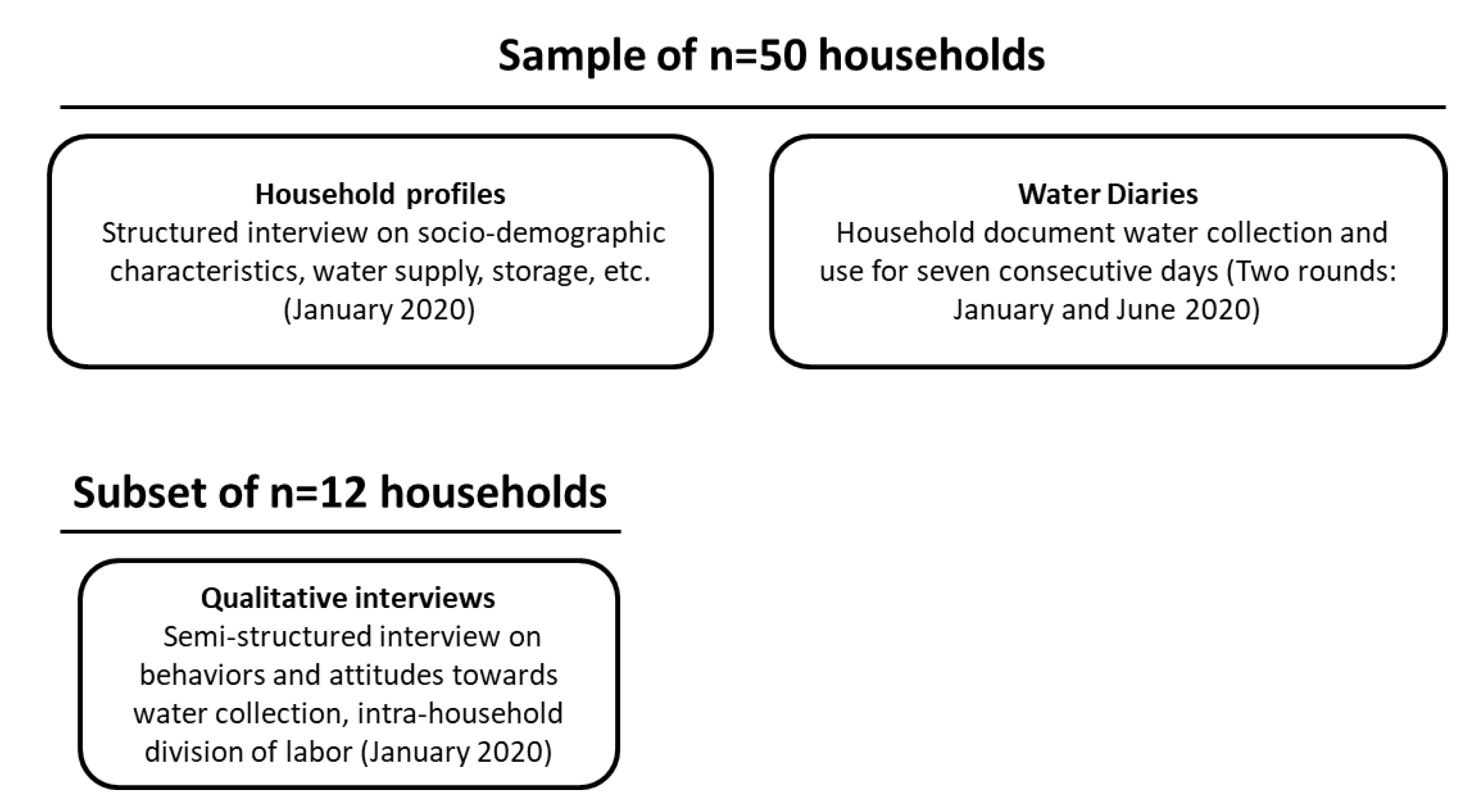
  • Household profile: Structured interview containing questions about socio-economic characteristics, such as size and composition of the household in terms of age and gender, income, and education levels. The interview included general questions about water access conditions, such as the frequency of piped supply, the availability and use of other supplies, water treatment practices, investments in storage vessels, and questions about health and livelihoods and their relationship to water. In addition, enumerators noted detailed information about ownership and capacity of water storage vessels, including buckets, plastic containers, tubs, and rooftop storage tanks
  • Water diaries: For seven consecutive days, the same households were given forms to document water collection by source and vessel type, for which each household was given options based on their available storage. The participants furthermore documented the use of water quantities for individual activities in their households. In collaboration with a graphic designer, pictograms for both the forms concerning water collection and use were developed and added in case participants were not able to read. The documentation of water collection and use for each day was split into three intra-daily time steps (morning, noon, and evening). The households were asked to time the duration of the entire water procurement process on each day, and to include only the time directly used for water procurement activities such as walking to the water source, waiting, filling vessels, and boiling water. The field team was conducting daily visits to the settlements to respond to questions of the participants and to collect the filled-out forms. Note that the implementation of the study in this form deviates from the initial plan for the diaries, which was adapted based on the feedback of households and enumerators. Originally, our study design closely matched the approach of Wutich [63] where households were given a standardized vessel to measure all water collection with. Additionally, we planned to ask households for a detailed timing of each abstraction of water. Both ideas were not accepted by the participants due to the extra effort involved (and would likely have led to contortions in the time measurements).
  • In-depth interviews: In 12 participating households, the profile and diary study were accompanied by a semi-structured, qualitative interview inquiring about water collection and use, water treatment practices, water-related diseases, responses to water-related uncertainty and emergency situations, subjective views on the development of water supply in the area, desires concerning water supply and the intra-household division of labor for both paid and unpaid work.

3.2.2. Second Stage of Field Studies in June 2020

A second stage of the diary study was carried out in June 2020, marking the dry pre-Monsoon part of the year, to account for seasonal effects. By this time, the COVID-19 pandemic had already severely affected Pune and most households were contained in a lock-down. Through community contact persons, the field team established telephonic contact with most of the participants from January. One household in the settlement Tarawade Vasti and all households in Janta Vasahat could not be contacted and were excluded from the second part of the study. In total, 41 households participated in the second stage of the study. These households consented to track their water collection and use for another seven days and being contacted daily by telephone to gather results. The effect of the pandemic on data quality is difficult to estimate because (1) the research approach had to be adjusted and (2) water supply and consumption patterns may have been affected by the lock-down. We therefore comment and speculate on seasonal differences in the next section but do not attempt to fully explain the June data or use it in our statistical models.

3.2.3. Verification and Analysis of Data

The retrieved water diary forms were recorded in tabular form and analyzed in the statistical software environment R [74]. A variety of consistency checks was employed to identify errors during data entry, such as typos in the transfer from the data form to the tables. The entries on water usage for household activities and the data on storage vessels were used to check the consistency of the entries on water collection and identify possible discrepancies. In cases where significant mismatches (>25 L) could not be explained by an error in the transfer of data, they were excluded from the analysis. Out of the 350 daily entries from January, seven had to be excluded due to unresolvable errors or because the participants did not fill out the diary from on this day. The in-depth interviews, originally conducted in Marathi with the help of a translator, were transcribed and translated verbatim into English. The transcripts were then coded using MAXQDA [75] to provide contextual descriptions (cf. Appendix A) and analyze patterns of water collection behavior, as described in the following section.

4. Household Profiles and Dynamics of Water Collection

In this section, we present an overview of the turnout of the household profile and diary study as well as relevant information for contextual understanding gathered in the in-depth interviews. The households in the sampled areas all used piped water services as their primary source of drinking water, either collected from a private connection, or a tap shared with neighbors and other households from the community. In all cases, female household members were responsible for water collection; sometimes this was carried out by one individual, sometimes it was considered a shared responsibility among female household members. In Table 2, an overview of demographic, socio-economic, and water-related characteristics of the sampled households is presented. As becomes apparent, there are strong differences among the settlements with regard to ownership of private network connections, storage capacities, and water-requiring facilities such as private bathrooms and toilets.

4.1. Water Supply Conditions and Collection Dynamics in the Sampled Settlements

The water supply situation in the five settlements and the water collection practices of participating households were assessed via the household profile survey and discussed in detail during the semi-structured interviews. Among and within settlements, considerable differences were found. In Appendix A, we present a short summary of the supply situation and supplement it with quotes from the qualitative interviews to characterize the situation of the participating households. Key insights retrieved through the interviews were:
  • Determinants of ability to collect network water: According to the interviewed households, the ability to collect water not only depends on the duration of piped supply and physical access to a tap, but quite crucially, on the flow rate of water. Water pressure differed considerably between days, among settlements, and even within these: Households located at a slope or the end of a heavily used pipe experienced very low flow rates and required considerably more time per collected unit of water. In other cases, one hour of supply was deemed sufficient to fill all storage vessels.
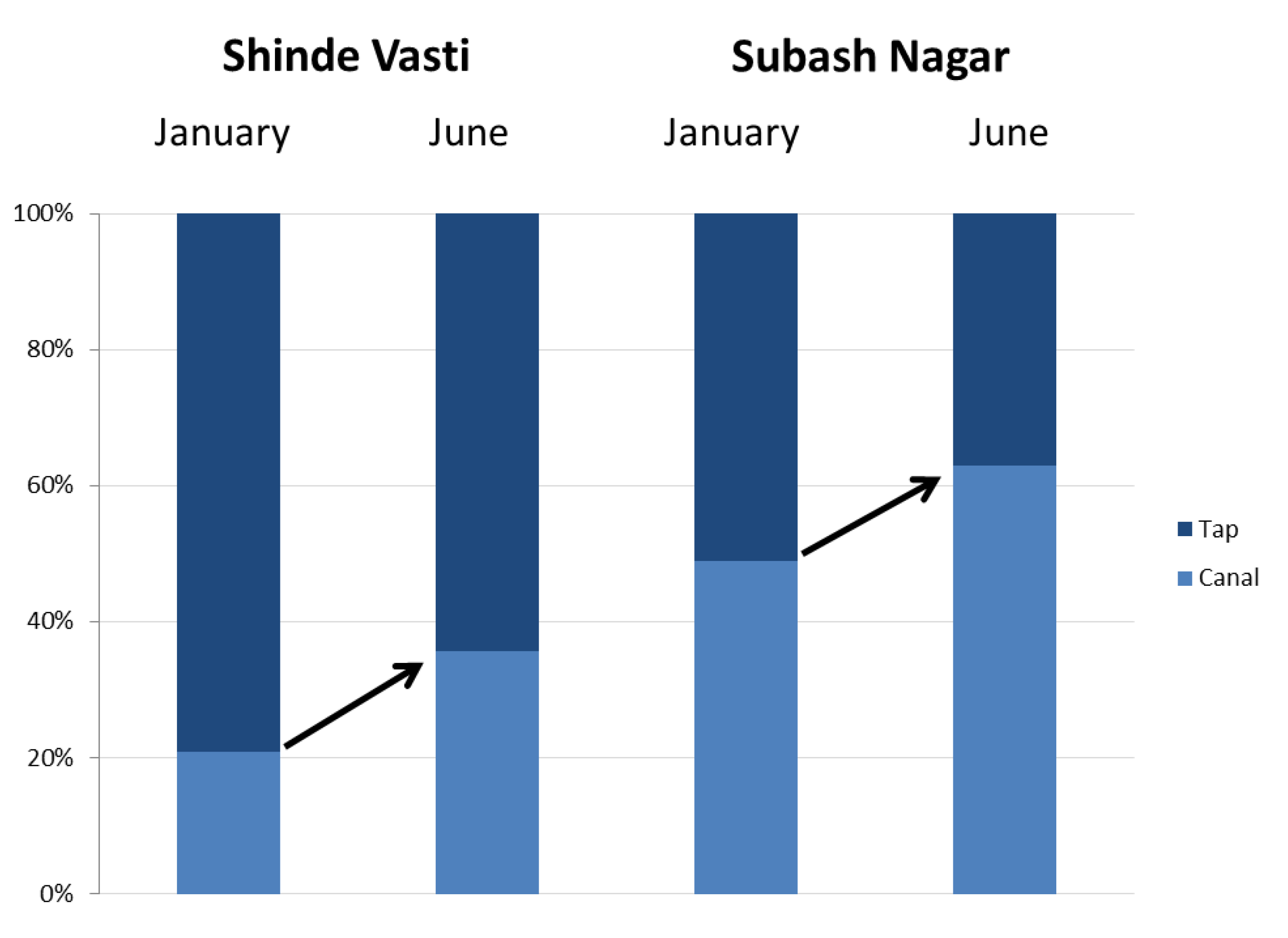
  • Seasonal changes of piped supply: The water supply situation present in January represents the most common situation throughout the year which may be referred to as “normal”, while the data collected in the dry pre-Monsoon phase characterizes a period with a duration of around one month. In addition, the interviews revealed that a third supply situation arises during Monsoon, which is characterized by ample availability of water but quality and acceptability issues, for instance, ‘muddy’ water. We, therefore, do not calculate average values per year in this or the next section but instead merely report the values for the two observed supply situations.
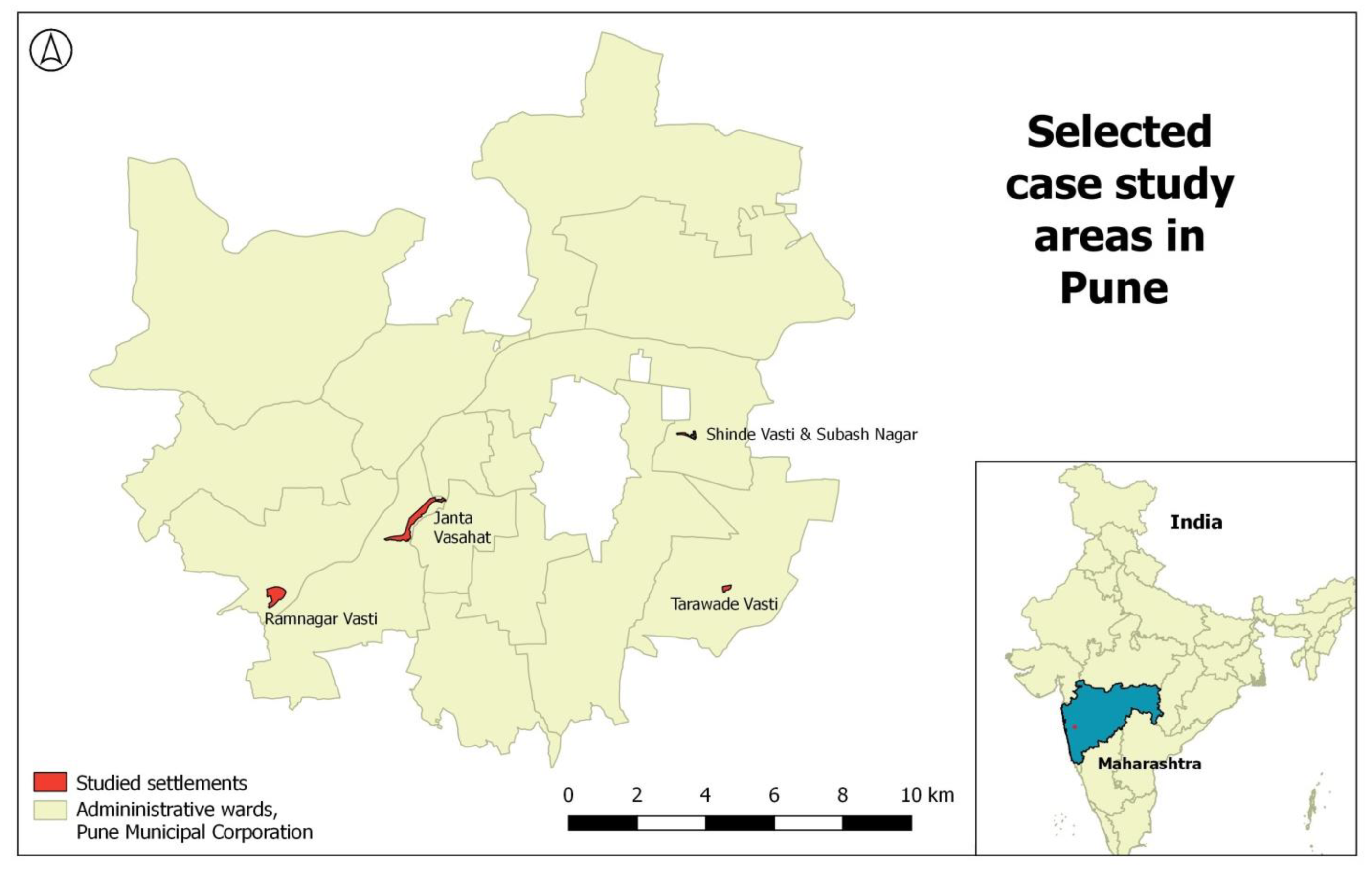
  • Use of multiple water sources: All interviewed households, with the exception of those residing in Janta Vasahat, claimed to either occasionally or regularly use supplementary sources of water. In the case of two settlements located in the vicinity of a canal (Shinde Vasti & Subash Nagar), surface water was used regularly for non-consumptive purposes such as washing and bathing.
  • Management of access to shared taps: For the households sharing water access points, two systems were found: In the case of a smaller number of households sharing one tap, property rights over time slots and a system of rotation at the tap were established to ensure equal access, resulting in an even distribution of procurement time. In the case of a high number of households sharing one public tap (in the settlement Subash Nagar), waiting times were less predictable as the system operated under the “first come, first served” principle.
  • Distinctions in quality levels: Among all participating households, the available storage capacity was divided into drinking and non-drinking storage, even if both were filled from the same piped network connection.

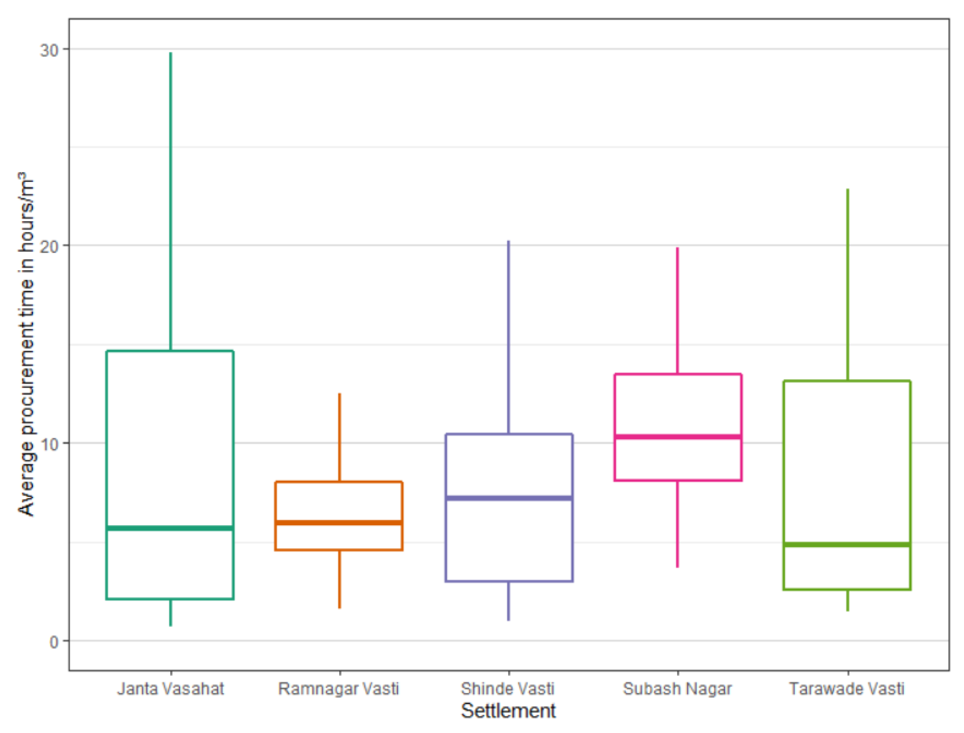
4.2. Time Expenditure for Water Procurement

The water diary data revealed substantial expenditures of household time with strong differences across settlements and respondents. The women of most households were found to spend up to several hours per day for water procurement. Table 3 summarizes key statistics of water procurement and consumption. Notably, the highest amount of the overall procurement time was spent filling storage vessels, including among households with in-house supplies.
In Figure 3, the distribution of time expenditure required to obtain one cubic meter of water by the different households within a settlement is presented. The graph demonstrates that variation within settlements is quite considerable and that even within a radius of a few hundred meters, water access conditions are quite diverse.

4.3. Seasonal Differences in Water Collection and Consumption

The interviews revealed that across all settlements, the service level of piped supply quality decreases in the pre-Monsoon time, in terms of supply duration, flow rate, and more frequent interruptions, leading to higher procurement time per collected unit. The diary data (see Table 3), however, only shows an increase in procurement time per cubic meter of water for two settlements (Ramnagar Vasti & Tarawade Vasti). This may be explained by the increased use of surface water in the other two settlements (Subash Nagar & Shinde Vasti) with data for both seasons. As Figure 4 illustrates, the residents of both areas consumed larger shares of canal water in June, which is available in close vicinity to their homes but of low quality and considered non-potable. By procuring more water from the canal, the residents increased their per capita water consumption in June, while decreasing procurement time. In contrast, the residents of areas without an easily available alternative reduced their consumption, despite higher temperatures, and required more time per unit of water.

5. Economic Analysis

5.1. The Economic Value of Water Procurement Time

In Section 2, we elaborated how unpaid work may be valued according to economic theory. In the following, we estimate the value of the opportunity cost of time in water procurement through wage rates, i.e., an input-based approach, as we are primarily concerned with the cost of procuring water from the perspective of an individual. In the next section, we briefly discuss the potential merits of an output-centered valuation. Due to the already intense participation of households, a stated preference experiment was deemed unfeasible as it would have used more time resources of participants and researchers.
The valuation was complicated by the employment situation of most participating households in our sample. None of the women in charge of water collection we interviewed were working as regularly employed wage earners with a formal hourly wage. Instead, most worked informally as domestic helpers, for which they earned salaries fixed for specific services rather than the time it takes to perform them. We found that the work situation of women in the sample was similar to the detailed description of Sarkar [76], who reports that domestic helpers in India are frequently working for several employers without a written contract or conventional methods of wage determination. Several women in the sample claimed to be self-employed, e.g., as waste pickers or vegetable re-sellers, and still, others claimed to not be engaged in any income-generating work. Across all cases, it was not clear if and how much marginal monetary income was foregone for allocating time to water collection. Thus, we opted to assign a range of three plausible values for one hour of work, namely
  • 14 INR/h, the average wage of an unskilled female laborer in urban centers of India [77]. This is our baseline value derived from the notion of neoclassical theory that the marginal value of time (even for leisure) corresponds to the marginal wage of an individual. We assume that the women participating in our study (including the self-employed individuals) would be able to obtain this wage, which is in fact below the minimum wage in urban Maharashtra [78].
  • 20 INR/h, which corresponds to half of the estimated earnings of one hour of work, which were established in the in-depth interviews with three participants who worked as domestic helpers. We chose to apply the 50%—assumption because it is commonly used in water collection studies [16,33];
  • 40 INR/h, which corresponds to 100% of the estimated wage from our interviews.
Among the literature dealing with water collection that was reviewed for this article, the case study of Amit und Sasidharan [36] in Chennai is likely to be the most comparable to ours, given that it is rather recent and set in urban India: Here, the authors used a wage rate of 30 INR per hour, which is in between our values (b) and (c). For each household, the average water procurement time per day and month was computed based on the seven diary entries in our collected data [41] and subsequently multiplied with all three wages. The results are compiled in Table 4. To categorize the results further, we grouped the sampled households into quartiles based on their average water procurement time: From the lowest average daily procurement time (min-Q1) to the highest (Q4-max), marking the right-most column in Table 4. To contextualize the relative significance of these estimates, we compared the time cost to two forms of income. First, the households’ reported monthly cash income, which is common in studies dealing with water collection costs. As Table 4 indicates, at the lowest assumed wage rate, the equivalent of 2.45–7.71% of monthly cash income is incurred as an opportunity cost of time. With the highest assumed wage rate, this value rises to 22.4% of cash income in the quartile of households with the highest procurement time per unit of water. The average share of time cost in cash income across the sample was 4.23% in January 2020, if the lowest wage rate is assumed. This figure and the measured water procurement time are comparable to the findings of Amit and Sasidharan [36] in Chennai, as well as to those of other coping cost studies in settings with high time costs [16,38]. When compared to conventional measures of affordability of water services, e.g., the commonly applied 5% of income thresholds [16,79,80], almost half of our sample has an affordability issue.
The expenditure we compare against this pecuniary budget, however, is not monetary in nature. Therefore, a theoretically more consistent budget to put time cost in proportion would be full income [19], i.e., the household’s time endowment valued at a marginal wage. Otherwise, as Uwera and Stage (2015, p. 10) have observed correctly, “one risks ending up with a situation where people ‘spend’ more on water than they have actually received in monetary terms”. Following their approach, we, therefore, computed a full income for each household in the sample [41], based on a time endowment of 24 h for each adult member of the household, while ignoring children below 18 years of age. Given that we value both the households’ entire time endowment and the time spent collecting water at the same wage rates, we can report the share of water procurement time in the overall time endowment independent of wage rate assumptions. Table 4 indicates that, on average, 2.36% of all household time per week is spent procuring water. In the quartile with the highest per unit procurement time, this value increases to 3.84% in January. The maximum value obtained for an individual household is 8.1% (not included in Table 4). While time cost computed as a percentage of the overall time endowment of the household results in a lower value than the share in monetary income, it is still a substantial cost when one considers that time for sleep, personal care, labor, and leisure are all allocated from this budget. Given that common measures of affordability use monetary income as a benchmark, we are not aware of a reference value or threshold to compare this figure against. In Section 6, we briefly discuss this issue further.
Finally, the computed time cost is compared anecdotally with the cost of other water services in Pune. In informal conversations during the field studies and merely for the purpose of comparison, we inquired about the price of home delivery of drinking water through tanker water services. If wage rate B (20 INR/h) is applied, the average household in our sample incurred time costs that are the rough equivalent of what a tanker water supplier would charge for the same quantity of water. This comparison, however, has clear limitations because tanker water services are often unavailable due to road conditions in informal settlements and frequently do not deliver small or marginal quantities of water.

5.2. Impact of Procurement Time on Consumed Quantity

The previous sections established that time costs are significant for many households in our sample. We hypothesized in Section 2 on the basis of household production theory that this cost should negatively impact the quantities consumed (Hypothesis 1). In the following, we investigate whether this is the case for the households in our sample. The seasonal variation in time expenditure per unit of water and the corresponding changes in consumed quantity, which were presented in Table 3 in the previous Section, tentatively point towards a negative correlation. To test the hypotheses developed in Section 2 with more robust methods, we developed four statistical models in which the response variable is the quantity of water consumed by a household on a specific day, independence of time expenditure per cubic meter of water, and other predictors such as income. Out of the January data [41], which was unaffected by the COVID-19 pandemic, we had n = 309 observations to draw from. Note that this number is lower than the 343 total data entries from January, as days without water supply (i.e., without procured quantity and procurement time) were excluded from the analysis, while they were used in the previous section to derive daily per capita consumption values. Analyzing repeated measurement data introduces non-independence but also allows controlling for unobserved, time-invariant variables such as household preferences. We use a multilevel approach, in particular a two-level mixed-effects model [81,82] of consumed quantity and time expenditure within households, which is common in diary studies [83]. We gradually increase the complexity of the models by adding observed time-invariant covariates such as the availability of a private network connection or income to the model and present four models with the highest level of fit. The estimated coefficients and key statistical information are compiled in Table 5, while we provide plots, compare information criteria (AIC/BIC), and test for collinearity and temporal autocorrelation in Appendix B.
Model A
Let t = 1 , , 7 days and i = 1 , ,   50 households. The following model is estimated:
ln ( y i t ) = α 0 + β 0 ln ( x i t ) + u i + ε i t
where y i t denotes the collected water quantity and x i t the procurement time of household i at day t , respectively. α 0 denotes the intercept, β 0 the slope of the model, while u i denotes unobserved effects at the household level, treated as random, and ε i t denotes the idiosyncratic error term.
Model B
Based on Model A, we now introduce settlement j = 1 , ,   5 as a second random effect to differentiate the variation between households in the model.
ln ( y i t ) = α 0 + β 0 ln ( x i t ) + u i + v j + ε i t
where v j denotes unobserved effects of settlement, treated as random.
Model C
Building on Model A once more, we now include the binary variable c i to the model to test for the effect of a piped network connection on both intercept and slope. c i is coded as a dummy variable with c i = 0 if a household has no private connection to the network and c i = 1 if it does have a connection.
ln ( y i t ) = α 0 + α 1 c i + β 0 ln ( x i t ) + β 1 c i ln ( x i t ) + u i + ε i t
where α 1 and β 1 denote the effect of c i   on intercept and slope, respectively.
Model D
Finally, we expand Model C to assess the implications of differences in the opportunity cost of time (Hypothesis 2). Because marginal wages for individual households in our sample could not be established (see above), and multiplication with an average or assumed wage adds no useful information to the model, we chose to apply the reported household cash income as a proxy for the opportunity cost of time. Thus, we add household monthly cash income I i   as a time-invariant covariate, resulting in the following composite model:
ln ( y i t ) = α 0 + α 1 c i + α 2 ln ( I i ) + β 0 ln ( x i t ) + β 1 c i ln ( x i t ) + β 2 ln ( I i ) ln ( x i t ) + u i + ε i t  
where α 2 and β 2 denote the effect of I i on intercept and slope, respectively.
The high significance, negative sign, and narrow confidence interval of the coefficient β 0 of water procurement time in Models A, B and C confirm the demand-reducing effect of time cost hypothesized in Section 2 (Hypothesis 1) with high significance. For Models A and B, β 0 can be directly interpreted as the elasticity of demand to procurement time and indicates that demand for water quantities is slightly inelastic to increasing time requirements. The effect of procurement time across all models provides further indication for the validity of the analytical conjectures made above on the basis of the stronger use of less time-intensive canal water in June (Figure 4).
Adding settlement as a random effect in Model B attributes a considerable part of variance to the area of residence, without losing substantial predictive accuracy. This may capture shared supply characteristics and potentially other unobserved variables that are similar in the area. For Models C and D, however, we removed v j as it decreased the level of fit. This may indicate that the predictors' connection c i and income I i capture at least partially what sets the respective settlements apart. By including c i into the model, the effect of procurement time can be further differentiated, albeit at the cost of a slightly wider confidence interval for β 0 . The coefficients β 0 and β 1   indicate that the demand of households with a private network connection is elastic to procurement time, while it is inelastic for those who do not have a connection. This can be explained by the ability of those with a private connection to better control when they use the tap and thus react more flexibly to fluctuations in procurement time, for instance when the flow rate of water is low. This explanation falls in line with information obtained during the in-depth interviews, where some respondents with a network connection claimed to avoid abstracting water while many of their neighbors do.
Adding household cash income to Model D makes the interpretation of the estimated coefficients less straightforward and introduced a higher degree of variability into the model. The results can nevertheless be interpreted as a confirmation for Hypothesis 2: Despite a wider confidence interval, a significant negative effect of income on the responsiveness to the opportunity cost of time is apparent, with a value of −0.28. For each 10% increase in income, the negative elasticity of the water collection quantity to procurement time is estimated to increase by 2.8%. This substantiates that those who we assume to have a higher opportunity cost of time indeed are more sensitive to procurement time as a determinant of demand. There may, however, be additional effects of higher income, such as an overall larger budget, which affect demand for water quantities and time savings. The modeled interaction effect between income and procurement time is thus not the only conceivable effect related to income. Wealthier households, for instance, may have chosen to live in a location with a more reliable and accessible piped supply or may have lobbied more effectively for those services to be provided in their neighborhoods. Nevertheless, our analysis contributes to explaining why higher-income households tend to rely on less time-intensive options to procure water quantities, such as larger storage capacities.

6. Discussion

By developing a novel form of water diary approach and applying it in a first case study in Pune, we obtained a unique sample of data on household time use to procure water. We found diverse water access conditions across five informal settlements, with considerable differences in frequency, duration, and pressure of water supply. These factors result in substantial water procurement time for many of the participating households. With or without network connections, household members can spend up to several hours per day filling storage vessels from low-pressure taps. Those that share communal taps spend additional time walking to these and waiting for their turn. These findings are in line with previous studies dealing with travel cost as part of water collection cost, for instance by Cook et al. [16] and Pattanayak et al. [38] in rural areas, or by Amit and Sasidharan [36] in urban India. While previous studies estimated a set of different coping costs or the effect of full cost on water demand, we focused exclusively on water procurement time and contributed to the first longitudinal study that provided repeated measurements over several days.
By applying three different wage rates to value the time households spend to obtain water, we were able to show that significant time costs of access to water are incurred by households in our sample, also by those who have a private network connection, and that these costs fluctuate considerably. We contextualized our valuations of water procurement time by comparing these against two household budgets. We found that time costs are substantial irrespective of the benchmark they are compared against. Depending on the applied wage rate, on average, households incurred time costs equivalent to 4.23–13.81% of their monthly cash income. When we compared time cost to the conceptually more sound full income or time endowment of the household, we find that the average household in our sample spends 2.36% of all the time available to adult household members for water procurement. Among households with particularly high time cost per unit of water, this figure can be up to 8.1%.
We then analyzed which implications time costs have for household water consumption. The multi-level models presented in the previous section confirmed our hypothesis that the opportunity cost of time has a significant and negative impact on demand for water quantities. Our basic model provides statistically robust evidence that household demand for water quantities is slightly inelastic (−0.90) to procurement time. To our knowledge, we have contributed the first analysis that isolates the effect of procurement time on demanded quantity, though others [29,30,31] had previously considered certain uses of time in the full cost predictor. Using an extended concept for time cost [21] we were able to show that the previous focus on walking to remote sources, however, is not comprehensive enough, as time expenditure can occur within the households’ residence as well. We differentiated our analysis through further models that grouped households by settlement, treated as a random effect, and by whether they have private network connections or not. We also investigated whether demand for water services is sensitive to individual differences in the opportunity cost of time, for which income was used as a proxy because we could not establish individual marginal values for the time of participating households. With an intermediate degree of confidence, due to more variability in this model, we were able to confirm that those with a higher opportunity cost of time respond more strongly to procurement time as a determinant of demand (2.38% increase in negative elasticity for every 10% increase of cash income). This finding has to be treated with higher care, as income may be endogenously related to other factors, such as the location of residence and the quality of supply there. Moreover, it is unclear whether the women in our sample could obtain market wages higher than the reservation wage of staying at home and procuring water.
Our findings substantiate that the time cost of water procurement should receive more attention in water policy, management and research. Across our sample, high time requirements of water collection contribute to a situation where households consume per capita quantities of water below-recommended minimum levels [42], with potentially adverse impacts on health. This substantiates that while piped water services might be provided free of monetary charges, they can still be quite “expensive” from the perspective of a household and do not necessarily result in a degree of access commensurate with the human right to water or Target 6.1. Currently used methods of assessing whether sufficient access to water exists, such as Indicator 6.1.1 of SDG 6, would not have diagnosed access issues for many households in this study. Can water be considered affordable if it takes hours to obtain comparatively small quantities? If time cost impacts the water quantities consumed by households—for which we found sound empirical evidence—there is a consistent explanation why households water would “underconsume” water supplied at no or low monetary charges [79]. The results of our analysis underscore a point others (e.g., [8]) have made before, namely that infrastructure availability does not guarantee adequate access to water. The focus of policymaking and monitoring should thus increasingly be placed on service levels, for those with and without network connections. Service levels and time costs should also receive more attention in research. More economists, for example, should attempt to incorporate time cost in water demand estimations in settings with no or low-quality water supply, if this is possible in terms of data, to avoid or reduce omitted variable bias. The recognition of the time variable may also lead to different assessments of welfare and rationales for policy, for example in funding decisions or cost-benefit analyses for service level improvements.
Our analysis is limited by a number of methodological issues. While we deliberately focused on water procurement time, we ignored other cost items and potentially relevant factors such as the physical effort associated with water collection or the health impacts of low-quality water. Moreover, the focus on time in household production omits management and planning tasks [43] as well as anxiety and stress that are the result of uncertainties about drinking water availability [84]. While our quantitative analyses did not differentiate water quality levels, their role in shaping demand for water services can be highly relevant [21,85]. The willingness of household members to invest time, for example, is likely to be higher for drinking purposes than for non-drinking water [17], as is the case with monetary expenditures [86]. We carried out this study in a unique setting where water services are provided free of monetary charges and did not focus in-depth on the impact of time cost on the selection of water sources, as most households in our sample used only one water source. In settings where multiple water sources are more frequently used and combined, however, the selection of source and quantitative demand should be considered jointly, and both monetary and time cost should influence decisions, as other studies [29,30] had shown previously. Our economic valuation of water procurement time suffers from ambiguity with respect to what the most accurate measure for the value of this time is. As Zhang et al. [53] (p. 64) have pointed out, for the case of travel time, “the value of incremental time savings would depend on opportunities to make use of the time saved”. This, however, is quite difficult to ascertain. Households in our study do not have the ability to flexibly choose between market work, household work, or leisure, which complicates the clear establishment of foregone opportunities. The wage rates we selected leave considerable room for interpretation as to which value best approximates the opportunity cost of time. This difficulty is not unique to our study: Cook et al. [16] (p. 857) note that “although households carrying water may incur large economic burdens, it is not easy for them to convert these economic costs into financial resources, i.e., convert saved time into money to pay vendors.” On a more fundamental level, it may be called into question whether procurement time is associated with disutility or has any value. Our household interviews revealed that while some households use water collection hours to socialize with neighbors, the majority clearly consider it burdensome. Gurung et al. [33] (p. 7085) reviewed studies of water collection and found “strong evidence that many households place a positive value on the time spent collecting”, i.e., that procurement time has an opportunity cost, even though individual valuations differ greatly and it is unclear whether time savings would be devoted to income-generating activities or leisure. From the perspective of households, time savings are likely beneficial irrespective of which activities they are reallocated to.
A limiting factor in our statistical analyses is that our data did not allow for the derivation of marginal procurement time, leading to the application of average values for the time expenditure per quantity obtained. For many of the participating households in this study, average and marginal procurement time do likely not differ considerably. Nevertheless, this issue is important to note as there are conceivable cases where this distinction matters, for example, if a household is deterred from enqueuing by a long line at the tap.
We are confident that the diary method produced high-quality data, in particular for the first round in January of 2020. The extent to which our study was impacted by the COVID-19 pandemic is difficult to ascertain, which is why we did not use the data from the (telephonic) second round of diaries in our statistical models and used it less extensively in our analyses. Notwithstanding this, the diary experiment proved to be useful for measuring both water consumption and time use with a high degree of accuracy. In our initial interviews, households were asked to roughly estimate their daily water consumption, which resulted in at times staggering differences to the values documented daily in the diaries, somewhat anecdotally confirming the more rigorous comparisons of data quality from different collection methods by Wutich [63] and Apoorva et al. [40]. The application of the diary method, however, has been resource-intensive when compared to a conventional household survey. Much training and communication as well as multiple rounds of refining the approach where required. With this amount of effort, we obtained a comparatively small data set, which is limited in transferability and representativeness. Water diaries are thus not a feasible alternative for standard surveys. They may, however, be useful in further investigating the dynamics of water collection and consumption in-depth in selected areas, for example, to develop an accurate understanding of access conditions or the effectiveness of specific interventions.
Future research should investigate in which way large-scale data collection efforts can efficiently and sufficiently account for the opportunity cost of time for water procurement. We showed that this may be essential to consider in certain contexts while monitoring the implementation of normative goals for water policy (SDG6, right to water). A potential solution between in-depth diaries and recall surveys may be the “Day Reconstruction Method” developed by Kahneman et al. [87]. Moreover, future research could analyze systematically which management practices effectively reduce water procurement time and to which extent this increases welfare. While there is no conclusive evidence that time savings due to improvements in water supply enhance female participation in labor markets [88,89,90], they have been shown to produce improved educational outcomes for children [91,92], thus offering the potential for synergies with other sustainability goals. While this article investigated the impact of time cost and water demand, many open questions remain about this relationship, such as the fluctuations of time cost throughout the seasons. For reasons outlined before, we did not analyze this in-depth due to the uncertain effect of the pandemic on our summer data, but increased water needs likely coincide with a higher physical effort of water collection during the hot months of the year. This point is of particular relevance against the background of climate change and its implications for residential water demand e.g., [93]. It could also be valuable to attempt an output-focused valuation [46] of time spent collecting water, i.e., not to investigate individual cost but the value added by households through the combination of time and market goods. Such attempts would be difficult for a range of reasons, for example, because no definable market good may be available as a benchmark or because input goods may be subsidized, as is the case in our study with piped supply. Nevertheless, an output valuation may produce quite different results than the analysis presented here and may be more suitable for cost-benefit analyses for the construction and operation of supply infrastructures.

7. Conclusions

Based on field studies in five informal settlements of Pune throughout the first half of 2020, we gathered high-resolution water consumption and time use data to analyze water procurement behaviors of households in areas where the conditions of access to water impose high time cost of walking, waiting and storing water. Our diary data revealed that the time households need to procure water differs considerably and is subject to fluctuations of supply and seasons. We analyzed this data with two objectives in mind: First, to assign monetary values to time cost and, second, to determine how this cost impacts the quantities of water consumed by households. The valuation of water procurement time was impeded by uncertainties about the appropriate marginal monetary value of household time, but it yielded substantial cost when expressed as a percentage in household cash income in any case: On average, time costs were equivalent to 4.23–13.81% of cash income, depending on the valuation method. When calculated as a share of the household time endowment, i.e., all time available to adults in the household, water procurement time amounts to 2.36% on average. Through a number of multi-level models, we were able to robustly confirm that water procurement time impacts how much water households consume in a significant way, with an elasticity of water consumption to procurement time of −0.90. These results substantiate two hypotheses we proposed based on economic literature: First, that water procurement time negatively impacts quantitative demand, and, secondly, that this relationship is stronger for households with a higher opportunity cost of time.
Time costs are likely to induce some of the households in our study to consume unhealthily small quantities of water. This underscores that they are a relevant issue to consider for water policy, particularly for Sustainable Development Goal 6 and the human right to water. If prohibitively high time requirements for accessing water reduce consumption below minimum levels required for health or impose unreasonable burdens, sufficient access is not granted, even though there may be infrastructure on the premises. In such cases, service levels have to be increased and factors such as duration, frequency, and flow rates of supply need to be considered. The nexus between time allocation and access to water should receive more attention in both water supply management and the research dedicated to it.

Author Contributions

Conceptualization, H.Z.; literature review, H.Z.; data collection and analysis, H.Z.; writing—original draft preparation, H.Z.; writing—review and editing, E.G., B.K., C.K. and H.Z.; supervision, E.G. All authors have read and agreed to the published version of the manuscript.

Funding

This work was conducted as part of the Belmont Forum Sustainable Urbanisation Global Initiative (SUGI)/Food-Water-Energy Nexus theme for which coordination was supported by the US National Science Foundation under grant ICER/EAR-1829999 to Stanford University. Also, as part of the Belmont Forum, the German Federal Ministry of Education and Research provided funding to the Helmholtz Centre for Environmental Research (UFZ) (033WU002). Any opinions, findings, conclusions, or recommendations expressed in this material do not necessarily reflect the views of the funding organizations.

Institutional Review Board Statement

Not applicable.

Informed Consent Statement

Not applicable.

Data Availability Statement

The data supporting our analysis and conclusions are cited in-text as [41]. Relevant data can be obtained from the Zenodo repository (https://zenodo.org, accessed on 17 March 2022; DOI: 10.5281/zenodo.5549665) under restricted access conditions due to the personal nature of the household profile data.

Acknowledgments

We would like to sincerely thank the entire team of the Maharashtra Social Housing and Action League (MASHAL) in Pune for their valuable contributions to the data collection for this study. In particular, we would like to thank Vishnu Shinde, Mandar Athvale, and Neeta Chalke. We dedicate this work to our friend and collaborator Sharad Mahajan, who passed away before he could see this published.

Conflicts of Interest

The authors declare no conflict of interest.

Appendix A

Table A1. Water supply conditions in the sampled settlements.
SettlementWater Supply Situation and Collection PracticesQuotes from Interviewees
Janta Vasahat (JV)All houses are reported to have their own water connection. The settlement is in the vicinity of a water treatment plant of Pune and supplied for several hours every day, except for Thursdays. The interviewees reported that water pressure is usually very stable. Some residents boil or treat the water before drinking it.There is no tension, water has a lot of pressure.
In summers, sometimes it comes, sometimes it doesn’t.
[About treating water with purifying chemicals] “In the rainy season, we add medicine in the water.”
Ramnagar Vasti (RN)The water supply situation differs throughout the settlement. The pucca houses at the bottom of the hill usually have private taps, whereas the residents of the kaccha houses located at the top of the hill share one connection among up to four households. Water is supplied for one hour per day in the early morning at a high flow rate. The households sharing a tap organize time slots for each to fill their vessel. If public supply is interrupted for a day or longer, the households fetch water from a large overhead tank located at the bottom of the hill.“Each house will fill [their water pots] for 15 min.”
“Everyday we change the first lady, we rotate to fill our pots.”
“If there is more water required, then I request the other person to manage and to give me some more time for fetching more water.”
[About Monsoon time] “Due to the rains water is dirty, at that time we usually boil it and then drink it.”
Shinde Vasti (SV)Most houses have a private water connection, while some inhabitants share taps with their neighbors in a yard. Water is supplied twice per day for two hours with at times low pressure. Some residents own electric pumps to transport the water into large storage tanks. In summer the water has a low flow rate and the supply hours are reduced. Some households use tanker water services during the summer months.The water is not clean, it has odor.
Water comes at 5 in the morning, I have to get up every day.”
In the summer, it comes for less for half an hour, with little pressure. Then I go to the canal to wash clothes
For a day, for three houses, we use one tanker.
Subash Nagar (SN)Water is supplied 2–3 times per day for about three hours to one tap which is shared by the entire community. Households reported quality issues with the tap water and at times health problems that they associated with it. The water connection has been provided by a private individual in exchange for a one-time payment.
Household members walk to the tap, wait and fill their vessels in order of appearance. Most households use the canal water for non-drinking activities. In the summer months, supply interruptions cause households to share water with neighbors and walk to boreholes or public taps which may be quite distant.
In summer, it happens a lot, for two days water doesn’t come. At that highway [roughly 1 km distance] there are some hotels, there is a tap, then we bring water from there.”
Whoever is the first one fills water first.”
The whole slum area fills water from there and we require one hour to fill our pots so we have to wait for a long time.”
I feel cramps in my legs because I have to come and go many times to draw water.”
In the rainy season mud comes in the water. [Then] I filter the water through a cloth.”
Tarawade Vasti (TV)Water is supplied every second day for a duration of two hours. The flow rate of the water differs considerably throughout the settlements. Those at higher altitudes reported to experience low water pressure, especially if others open their taps. Households typically own large storage tanks either on the roof or next to their building.
In summer, supply interruptions cause residents to walk to a nearby larger road and carry water from a tanker truck home.
“Every house here has a tap of their own.”
[When supply is interrupted unexpectedly] “We fill on some other person’s tap, we do not get enough water. Minimum 5 h go to fetching water from there.”
[In summer] “I do not wash the clothes also sometimes I don’t bath the children.”
[In summer] “Sometimes a lot of quarrels happen”
“After drinking this water children have problems, stomach ache, vomiting.”

Appendix B. Plots and Model Fit Diagnostics

In this section, we present plots, exemplary calculations, and additional model diagnostics to assess the level of fit for the models developed in Section 5.

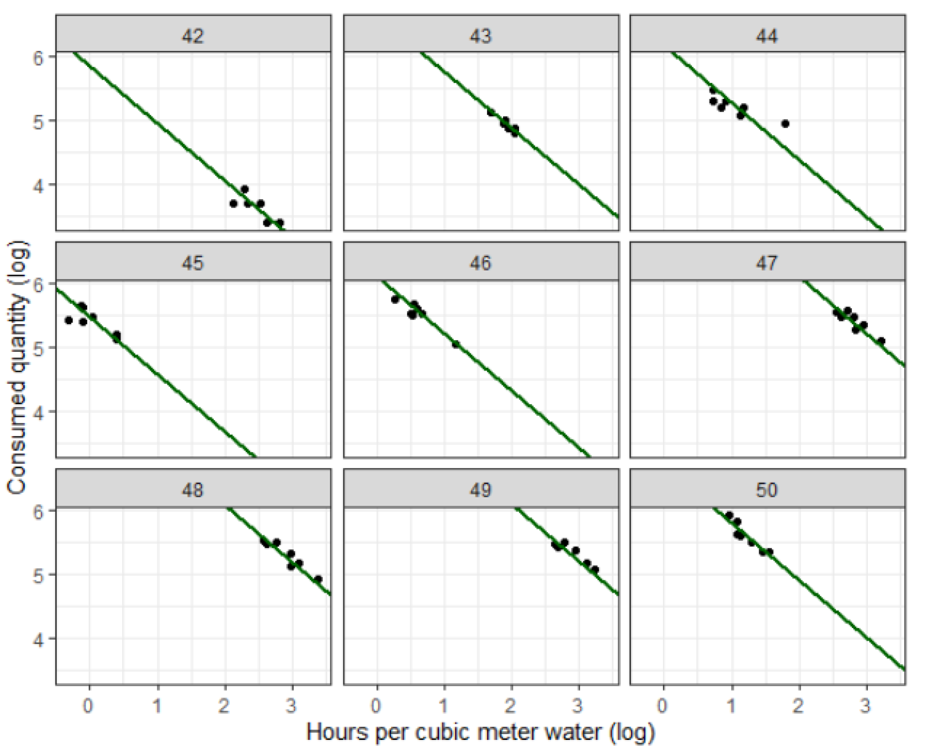
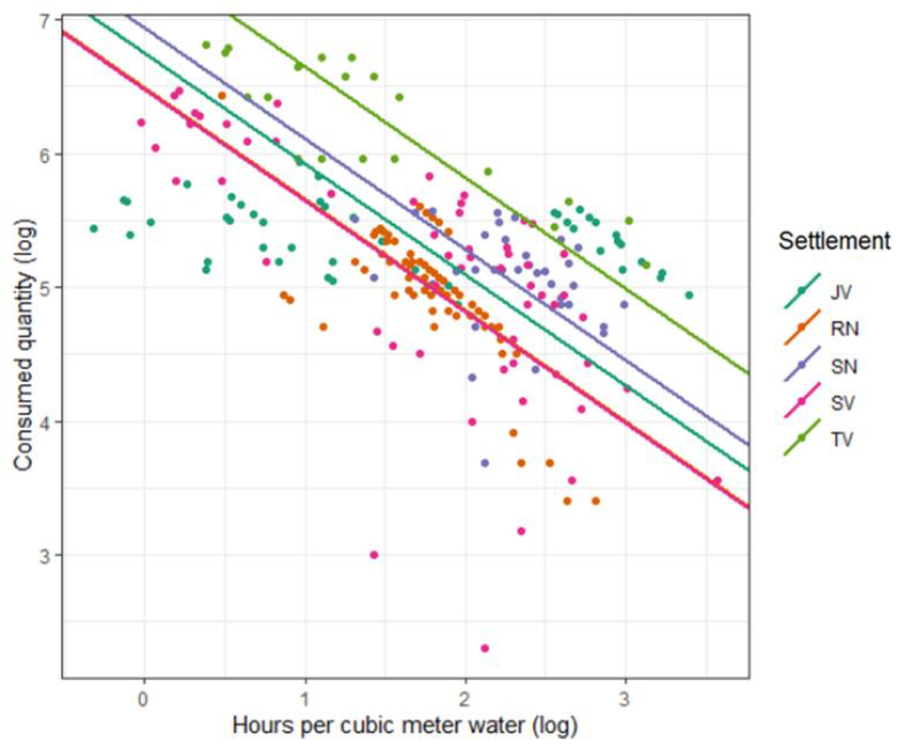
Appendix B.1. Data and Model Plots

Figure A1. Consumed quantity of water for each measured day against the procurement time, calculated in hours per cubic meter.
Water 14 01009 g0a1
Figure A2. Log-transformed data points of nine households and the fitted regression line for Model A, to illustrate the variability introduced by the random intercepts.
Water 14 01009 g0a2
Figure A3. The effect of the settlement on the intercept estimated in Model B. Note that the Figure does not display the variation on the household level even though this is included in the model. Also note that the fitted lines for settlements RN and JV have almost identical shapes, such that RN is not visible in this plot.
Water 14 01009 g0a3

Appendix B.2. Model Diagnostics & Fit

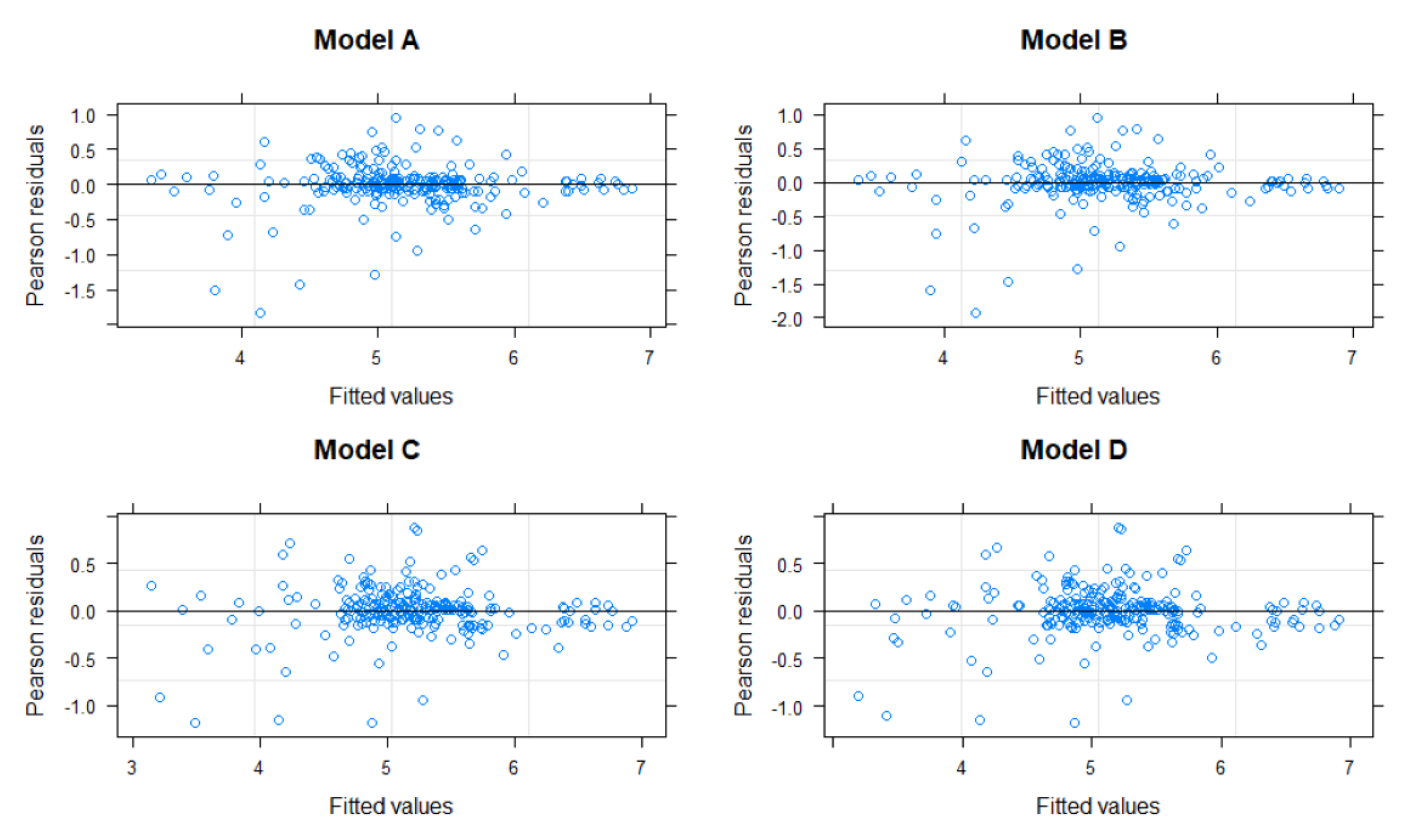
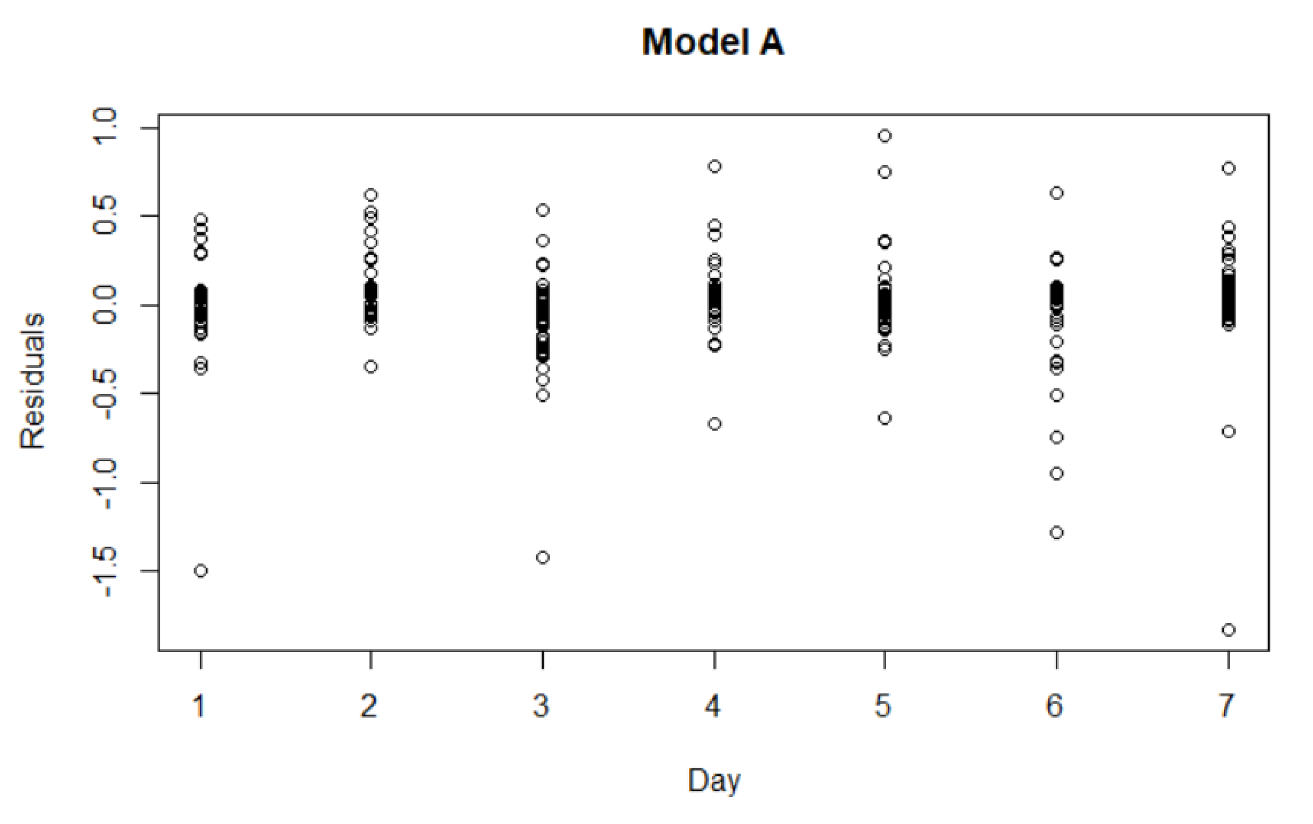
Appendix B.2.1. Residuals

The model residuals (Figure A4) indicated no clear deviations from the linear form and a relatively constant variance across the range of fitted values.
Figure A4. Residuals plotted against fitted model values.
Water 14 01009 g0a4

Appendix B.2.2. Temporal Autocorrelation

In Figure A5, residuals were plotted against the day of measurement to test for temporal autocorrelation in the data. The graph indicates that there may be temporal autocorrelation to a limited extent, but no clear trend is visible.
Figure A5. Residuals plotted by day.
Water 14 01009 g0a5

Appendix B.2.3. Multicollinearity

To test for multicollinearity among the independent variables in Models C and D, variance inflation factors (VIF) with a cut-off value of 5 were calculated (with the exception of interaction terms, where VIF does not apply). The VIF of the independent variables in Models C and D were found to be between 1.3 and 2.9, indicating the absence of strong collinearity.

Appendix B.2.4. Information Criteria

We used the Akaike Information Criterion (AIC) and the Bayesian Information Criterion (BIC) to compare the goodness of fit across models. As Table 5 in Section 5 indicates, the values of AIC and BIC decreased across Models A to C, i.e., each model increased the level of fit over the previous forms. Model D was estimated using a slightly smaller data set (n = 298) because two households did not report income. To compare the goodness of fit of Model D to Models A to C, we, therefore, excluded these data points from the other models. Table A2 indicates the goodness of fit for all four models using n = 298 data points. The results indicate that while Model D may be useful for investigating Hypothesis 2, it decreases the goodness of fit to include income into the model.
Table A2. Information criteria.
ModelAkaike Information Criterion (AIC)Bayesian Information Criterion (BIC)
A320.707 335.495
B308.738327.224
C256.431278.614
D258.884 288.461

References

  1. United Nations General Assembly. The Human Right to Water and Sanitation; UNGA: New York, NY, USA, 2010. [Google Scholar]
  2. UN-Water. Progress Over Time of Indicator 6.1.1—Proportion of Population Using Safely Managed Drinking Water Services. Available online: https://www.sdg6data.org/indicator/6.1.1 (accessed on 3 February 2022).
  3. Gawel, E.; Bretschneider, W. Sustainable access to water for all: How to conceptualize and to implement the human right to water. J. Eur. Environ. Plan. Law 2016, 13, 190–217. [Google Scholar] [CrossRef]
  4. Giné Garriga, R.; Pérez Foguet, A. Water, sanitation, hygiene and rural poverty: Issues of sector monitoring and the role of aggregated indicators. Water Policy 2013, 15, 1018–1045. [Google Scholar] [CrossRef]
  5. Nganyanyuka, K.; Martinez, J.; Wesselink, A.; Lungo, J.H.; Georgiadou, Y. Accessing water services in Dar es Salaam: Are we counting what counts? Habitat Int. 2014, 44, 358–366. [Google Scholar] [CrossRef]
  6. Guppy, L.; Mehta, P.; Qadir, M. Sustainable development goal 6: Two gaps in the race for indicators. Sustain. Sci. 2019, 14, 501–513. [Google Scholar] [CrossRef]
  7. De Albuquerque, C. Realising the Human Rights to Water and Sanitation: A Handbook/By the UN Special Rapporteur Catarina de Albuquerque; United Nations: Bangalore, India, 2014; ISBN 978-989-20-4980-9. [Google Scholar]
  8. Moriarty, P.; Smits, S.; Butterworth, J.; Franceys, R. Trends in Rural Water Supply: Towards a Service Delivery Approach. Water Altern. 2013, 6, 329–349. [Google Scholar]
  9. Gawel, E.; Bretschneider, W. Specification of a human right to water: A sustainability assessment of access hurdles. Water Int. 2017, 42, 505–526. [Google Scholar] [CrossRef]
  10. Rawas, F.; Bain, R.; Kumpel, E. Comparing utility-reported hours of piped water supply to households’ experiences. Npj Clean Water 2020, 3, 6. [Google Scholar] [CrossRef] [Green Version]
  11. Majuru, B.; Suhrcke, M.; Hunter, P.R. How do households respond to unreliable water supplies? A systematic review. Int. J. Environ. Res. Public Health 2016, 13, 1222. [Google Scholar] [CrossRef] [Green Version]
  12. O’Donnell, E.L.; Garrick, D.E. The diversity of water markets: Prospects and perils for the SDG agenda. Wiley Interdiscip. Rev. Water 2019, 6, e1368. [Google Scholar] [CrossRef]
  13. Zozmann, H.; Klassert, C.; Sigel, K.; Gawel, E.; Klauer, B. Commercial Tanker Water Demand in Amman, Jordan—A Spatial Simulation Model of Water Consumption Decisions under Intermittent Network Supply. Water 2019, 11, 254. [Google Scholar] [CrossRef] [Green Version]
  14. Klassert, C.; Sigel, K.; Gawel, E.; Klauer, B. Modeling residential water consumption in Amman: The role of intermittency, storage, and pricing for piped and tanker water. Water 2015, 7, 3643–3670. [Google Scholar] [CrossRef] [Green Version]
  15. Sarkar, A. Everyday practices of poor urban women to access water: Lived realities from a Nairobi slum. Afr. Stud. 2020, 79, 212–231. [Google Scholar] [CrossRef]
  16. Cook, J.; Kimuyu, P.; Whittington, D. The costs of coping with poor water supply in rural Kenya. Water Resour. Res. 2016, 52, 841–859. [Google Scholar] [CrossRef] [Green Version]
  17. Aini, M.S.; Fakhrul-Razi, A.; Mumtazah, O.; Chen, J.M. Malaysian households’ drinking water practices: A case study. Int. J. Sustain. Dev. World Ecol. 2007, 14, 503–510. [Google Scholar] [CrossRef]
  18. Thompson, J.; Porras, I.T.; Wood, E.; Tumwine, J.K.; Mujwahuzi, M.R.; Katui-Katua, M.; Johnstone, N. Waiting at the tap: Changes in urban water use in East Africa over three decades. Environ. Urban. 2000, 12, 37–52. [Google Scholar] [CrossRef]
  19. Becker, G.S. A Theory of the Allocation of Time. Econ. J. 1965, 75, 493–517. [Google Scholar] [CrossRef] [Green Version]
  20. Komarulzaman, A.; de Jong, E.; Smits, J. Hidden water affordability problems revealed in developing countries. J. Water Resour. Plan. Manag. 2019, 145, 5019006. [Google Scholar] [CrossRef]
  21. Zozmann, H.; Klassert, C.; Klauer, B.; Gawel, E. Heterogeneity, household co-production, and risks of water services—Water demand of private households with multiple water sources. Water Econ. Policy 2022, accepted. [Google Scholar]
  22. Bretschneider, W. Versorgungsgerechtigkeit in einer nachhaltigen Trinkwasserwirtschaft: Ein institutionenökonomischer Ansatz zur Berücksichtigung des sozialen Anliegens im Zielfächer der Wasserpolitik. Ph.D. Thesis, Leipzig University, Leipzig, Germany, 2016. [Google Scholar]
  23. Price, H.; Adams, E.; Quilliam, R.S. The difference a day can make: The temporal dynamics of drinking water access and quality in urban slums. Sci. Total Environ. 2019, 671, 818–826. [Google Scholar] [CrossRef]
  24. UNICEF. Thirsting for a Future: Water and Children in a Changing Climate; UNICEF: New York, NY, USA, 2017; ISBN 9280648748. [Google Scholar]
  25. Chen, Y.J.; Chindarkar, N.; Zhao, J. Water and time use: Evidence from Kathmandu, Nepal. Water Policy 2019, 21, 76–100. [Google Scholar] [CrossRef]
  26. Gross, E.; Elshiewy, O. Choice and quantity demand for improved and unimproved public water sources in rural areas: Evidence from Benin. J. Rural Stud. 2019, 69, 186–194. [Google Scholar] [CrossRef]
  27. Nauges, C.; van den Berg, C. Demand for Piped and Non-piped Water Supply Services: Evidence from Southwest Sri Lanka. Env. Resour. Econ. 2009, 42, 535–549. [Google Scholar] [CrossRef]
  28. Cheesman, J.; Bennett, J.; Son, T.V.H. Estimating household water demand using revealed and contingent behaviors: Evidence from Vietnam. Water Resour. Res. 2008, 44, W11428. [Google Scholar] [CrossRef]
  29. Uwera, C.; Stage, J. Water Demand by Unconnected Urban Households in Rwanda. Water Econ. Policy 2015, 1, 1450002. [Google Scholar] [CrossRef]
  30. Nauges, C.; Strand, J. Estimation of non-tap water demand in Central American cities. Resour. Energy Econ. 2007, 29, 165–182. [Google Scholar] [CrossRef]
  31. Acharya, G.; Barbier, E. Using Domestic Water Analysis to Value Groundwater Recharge in the Hadejia’Jama’are Floodplain, Northern Nigeria. Am. J. Agric. Econ. 2002, 84, 415–426. [Google Scholar] [CrossRef]
  32. Pattanayak, S.; Yang, J.-C.; Whittington, D.; Bal Kumar, K.C. Coping with unreliable public water supplies: Averting expenditures by households in Kathmandu, Nepal. Water Resour. Res. 2005, 41, 1–11. [Google Scholar] [CrossRef] [Green Version]
  33. Gurung, Y.; Zhao, J.; Kumar KC, B.; Wu, X.; Suwal, B.; Whittington, D. The costs of delay in infrastructure investments: A comparison of 2001 and 2014 household water supply coping costs in the Kathmandu Valley, Nepal. Water Resour. Res. 2017, 53, 7078–7102. [Google Scholar] [CrossRef] [Green Version]
  34. Bernard, H.R.; Killworth, P.; Kronenfeld, D.; Sailer, L. The problem of informant accuracy: The validity of retrospective data. Annu. Rev. Anthropol. 1984, 13, 495–517. [Google Scholar] [CrossRef]
  35. Vásquez, W.F. Reliability perceptions and water storage expenditures: Evidence from Nicaragua. Water Resour. Res. 2012, 48, 1–8. [Google Scholar] [CrossRef] [Green Version]
  36. Amit, R.K.; Sasidharan, S. Measuring affordability of access to clean water: A coping cost approach. Resour. Conserv. Recycl. 2019, 141, 410–417. [Google Scholar] [CrossRef]
  37. Whittington, D.; Mu, X.; Roche, R. Calculating the value of time spent collecting water: Some estimates for Ukunda, Kenya. World Dev. 1990, 18, 269–280. [Google Scholar] [CrossRef]
  38. Pattanayak, S.; Poulos, C.; Yang, J.-C.; Patil, S.R. How valuable are environmental health interventions? Evidence from a quasi-experimental evaluation of community water projects. Bull. World Health Organ. 2010, 88, 535–542. [Google Scholar] [CrossRef] [PubMed]
  39. Dongzagla, A.; Nunbogu, A.M.; Fielmua, N. Does self-reported water collection time differ from observed water collection time? Evidence from the Upper West Region of Ghana. J. Water Sanit. Hyg. Dev. 2020, 10, 357–365. [Google Scholar] [CrossRef]
  40. Apoorva, R.; Biswas, D.; Srinivasan, V. Do household surveys estimate tap water use accurately? Evidence from pressure-sensor based estimates in Coimbatore, India. J. Water Sanit. Hyg. Dev. 2018, 8, 278–289. [Google Scholar] [CrossRef]
  41. Zozmann, H. Household Profiles and Water Diary Data from Five Informal Settlements in Pune, India. Available online: https://zenodo.org/record/5549665#.YWAQBd9CSUk (accessed on 8 October 2021).
  42. Gleick, P.H. The human right to water. Water Policy 1998, 1, 487–503. [Google Scholar] [CrossRef]
  43. MacDonald, M. Feminist economics: From theory to research. Can. J. Econ. 1995, 18, 159–176. [Google Scholar] [CrossRef]
  44. Reid, M.G. Economics of Household Production; J. Wiley & Sons: New York, NY, USA, 1934. [Google Scholar]
  45. Posnett, J.; Jan, S. Indirect cost in economic evaluation: The opportunity cost of unpaid inputs. Health Econ. 1996, 5, 13–23. [Google Scholar] [CrossRef]
  46. Goldschmidt-Clermont, L. Output-Related Evaluations of Unpaid Household Work: A Challenge for Time Use Studies. Home Econ. Res. J. 1983, 12, 127–132. [Google Scholar] [CrossRef]
  47. Koopmanschap, M.A.; van Exel, N.; Job, A.; van den Berg, B.; Brouwer, W.B.F. An overview of methods and applications to value informal care in economic evaluations of healthcare. Pharmacoeconomics 2008, 26, 269–280. [Google Scholar] [CrossRef]
  48. Drummond, M.F.; Sculpher, M.J.; Claxton, K.; Stoddart, G.L.; Torrance, G.W. Methods for the Economic Evaluation of Health Care Programmes; Oxford University Press: Oxford, UK, 2015; ISBN 0191643580. [Google Scholar]
  49. Goldschmidt-Clermont, L. Monetary Valuation of Non-Market Productive Time Methodological Considerations. Rev. Income Wealth 1993, 39, 419–433. [Google Scholar] [CrossRef]
  50. Kulshreshtha, A.C.; Singh, G. Valuation of Non-Market Household Production, New Delhi: India, 1999. Available online: https://www.undp.org/content/dam/india/docs/valuation_non_market_household_production.pdf (accessed on 17 March 2022).
  51. Krol, M.; Brouwer, W. Unpaid work in health economic evaluations. Soc. Sci. Med. 2015, 144, 127–137. [Google Scholar] [CrossRef] [PubMed]
  52. Boardman, A.E.; Greenberg, D.H.; Vining, A.R.; Weimer, D.L. Cost-Benefit Analysis; Cambridge University Press: Cambridge, UK, 2018. [Google Scholar]
  53. Zhang, A.; Boardman, A.E.; Gillen, D.; Waters, I. Towards Estimating the Social and Environmental Costs of Transportation in Canada; The University of British Columbia, Centre for Transportation Studies: Vancouver, BC, Canada, 2004. [Google Scholar]
  54. Whittington, D.; Cook, J. Valuing changes in time use in low-and middle-income countries. J. Benefit-Cost Anal. 2019, 10, 51–72. [Google Scholar] [CrossRef] [PubMed] [Green Version]
  55. White, G.F.; Bradley, D.J.; White, A.U. Drawers of Water: Domestic Water Use in East Africa; University of Chicago Press: Chicago, IL, USA, 1972. [Google Scholar]
  56. Persson, T.H. Household choice of drinking–water source in the Philippines. Asian Econ. J. 2002, 16, 303–316. [Google Scholar] [CrossRef]
  57. Wagner, J.; Cook, J.; Kimuyu, P. Household demand for water in rural Kenya. Environ. Resour. Econ. 2019, 74, 1563–1584. [Google Scholar] [CrossRef]
  58. Prochaska, F.J.; Schrimper, R.A. Opportunity cost of time and other socioeconomic effects on away-from-home food consumption. Am. J. Agric. Econ. 1973, 55, 595–603. [Google Scholar] [CrossRef]
  59. Laughland, A.S.; Musser, L.M.; Musser, W.N.; Shortle, J.S. The opportunity cost of time and averting expenditures for safe drinking water. JAWRA J. Am. Water Resour. Assoc. 1993, 29, 291–299. [Google Scholar] [CrossRef]
  60. World Bank. World Development Report 1994. Infrastructure for Development; Oxford University Press: Oxford, UK, 1994; ISBN 0-19-520992-3. [Google Scholar]
  61. Elliott, M.; Foster, T.; MacDonald, M.C.; Harris, A.R.; Schwab, K.J.; Hadwen, W.L. Addressing how multiple household water sources and uses build water resilience and support sustainable development. Npj Clean Water 2019, 2, 1–5. [Google Scholar] [CrossRef] [Green Version]
  62. Tamason, C.C.; Bessias, S.; Villada, A.; Tulsiani, S.M.; Ensink, J.H.J.; Gurley, E.S.; Mackie Jensen, P.K. Measuring domestic water use: A systematic review of methodologies that measure unmetered water use in low-income settings. Trop. Med. Int. Health 2016, 21, 1389–1402. [Google Scholar] [CrossRef]
  63. Wutich, A. Estimating household water use: A comparison of diary, prompted recall, and free recall methods. Field Methods 2009, 21, 49–68. [Google Scholar] [CrossRef]
  64. Subbaraman, R.; Shitole, S.; Shitole, T.; Sawant, K.; O’brien, J.; Bloom, D.E.; Patil-Deshmukh, A. The social ecology of water in a Mumbai slum: Failures in water quality, quantity, and reliability. BMC Public Health 2013, 13, 173. [Google Scholar] [CrossRef] [PubMed] [Green Version]
  65. Kumpel, E.; Woelfle-Erskine, C.; Ray, I.; Nelson, K.L. Measuring household consumption and waste in unmetered, intermittent piped water systems. Water Resour. Res. 2017, 53, 302–315. [Google Scholar] [CrossRef] [Green Version]
  66. World Health Organization. Core Questions on Drinking Water and Sanitation for Household Surveys; World Health Organization: Geneva, Switzerland, 2006; ISBN 9241563265. [Google Scholar]
  67. Hoque, S.F.; Hope, R. The water diary method–proof-of-concept and policy implications for monitoring water use behaviour in rural Kenya. Water Policy 2018, 20, 725–743. [Google Scholar] [CrossRef]
  68. Hoque, S.F.; Hope, R. Examining the economics of affordability through water diaries in coastal Bangladesh. Water Econ. Policy 2020, 6, 1950011. [Google Scholar] [CrossRef]
  69. Bishop, S. Using water diaries to conceptualize water use in Lusaka, Zambia. ACME Int. J. Crit. Geogr. 2015, 14, 688–699. [Google Scholar]
  70. Masuda, Y.J.; Fortmann, L.; Gugerty, M.K.; Smith-Nilson, M.; Cook, J. Pictorial approaches for measuring time use in rural Ethiopia. Soc. Indic. Res. 2014, 115, 467–482. [Google Scholar] [CrossRef] [PubMed] [Green Version]
  71. Davis, J.; Crow, B.; Miles, J. Measuring water collection times in Kenyan informal settlements. In Proceedings of the Fifth International Conference on Information and Communication Technologies and Development, Atlanta, GA, USA, 12–15 March 2012; pp. 114–121. [Google Scholar]
  72. Ho, J.C.; Russel, K.C.; Davis, J. The challenge of global water access monitoring: Evaluating straight-line distance versus self-reported travel time among rural households in Mozambique. J. Water Health 2014, 12, 173–183. [Google Scholar] [CrossRef]
  73. Gershuny, J.; Harms, T.; Doherty, A.; Thomas, E.; Milton, K.; Kelly, P.; Foster, C. Testing self-report time-use diaries against objective instruments in real time. Sociol. Methodol. 2020, 50, 318–349. [Google Scholar] [CrossRef] [Green Version]
  74. R Core Team. R: A Language and Environment for Statistical Computing. Available online: https://www.R-project.org/ (accessed on 5 January 2022).
  75. VERBI Software. MAXQDA, Software for Qualitative Data Analysis, 1989–2012; Sozialforschung GmbH: Berlin, Germany, 2012. [Google Scholar]
  76. Sarkar, K. Complexity in the Determination of Minimum Wages for Domestic Workers in India; V.V. Giri national Labour Institute: Noida, India, 2019; ISBN 978-93-82902-65-2. [Google Scholar]
  77. National Sample Survey Office. Employment and Unemployment Situation in India: NSS Report No. 554 (68/10/1); National Sample Survey Office: Delhi, India, 2014. [Google Scholar]
  78. Workforce Consulting. Minimum wages in Maharashtra w.e.f. 1-July-2020. Available online: https://workforce.org.in/blog/maharashtra-minimum-wages-july-2020/ (accessed on 21 June 2021).
  79. Gawel, E.; Sigel, K.; Bretschneider, W. Affordability of water supply in Mongolia: Empirical lessons for measuring affordability. Water Policy 2013, 15, 19–42. [Google Scholar] [CrossRef]
  80. Hutton, G. Monitoring “Affordability” of Water and Sanitation Services after 2015: Review of Global Indicator Options; A Paper Submitted to the UN Office of the High Commissioner for Human Rights; World Health Organization: Geneva, Switzerland, 2012. [Google Scholar]
  81. Goldstein, H. Multilevel Statistical Models; John Wiley & Sons: Hoboken, NJ, USA, 2011; ISBN 111995682X. [Google Scholar]
  82. Kreft, I.G.G.; Kreft, I.; de Leeuw, J. Introducing Multilevel Modeling; SAGE Publishing: Newbury Park, CA, USA, 1998; ISBN 0761951415. [Google Scholar]
  83. Bolger, N.; Davis, A.; Rafaeli, E. Diary methods: Capturing life as it is lived. Annu. Rev. Psychol. 2003, 54, 579–616. [Google Scholar] [CrossRef] [Green Version]
  84. Wutich, A.; Ragsdale, K. Water insecurity and emotional distress: Coping with supply, access, and seasonal variability of water in a Bolivian squatter settlement. Soc. Sci. Med. 2008, 67, 2116–2125. [Google Scholar] [CrossRef] [PubMed]
  85. Rosenberg, D.E.; Tarawneh, T.; Abdel-Khaleq, R.; Lund, J.R. Modeling integrated water user decisions in intermittent supply systems. Water Resour. Res. 2007, 43, W07425. [Google Scholar] [CrossRef]
  86. Grupper, M.A.; Schreiber, M.E.; Sorice, M.G. How Perceptions of Trust, Risk, Tap Water Quality, and Salience Characterize Drinking Water Choices. Hydrology 2021, 8, 49. [Google Scholar] [CrossRef]
  87. Kahneman, D.; Krueger, A.B.; Schkade, D.A.; Schwarz, N.; Stone, A.A. A survey method for characterizing daily life experience: The day reconstruction method. Science 2004, 306, 1776–1780. [Google Scholar] [CrossRef] [PubMed]
  88. Meeks, R.C. Water works the economic impact of water infrastructure. J. Hum. Resour. 2017, 52, 1119–1153. [Google Scholar] [CrossRef] [Green Version]
  89. Devoto, F.; Duflo, E.; Dupas, P.; Parienté, W.; Pons, V. Happiness on tap: Piped water adoption in urban Morocco. Am. Econ. J. Econ. Policy 2012, 4, 68–99. [Google Scholar] [CrossRef] [Green Version]
  90. Gross, E.; Günther, I.; Schipper, Y. Women are walking and waiting for water: The time value of public water supply. Econ. Dev. Cult. Chang. 2018, 66, 489–517. [Google Scholar] [CrossRef] [Green Version]
  91. Koolwal, G.; van de Walle, D. Access to water, women’s work, and child outcomes. Econ. Dev. Cult. Chang. 2013, 61, 369–405. [Google Scholar] [CrossRef] [Green Version]
  92. Nauges, C.; Strand, J. Water hauling and girls’ school attendance: Some new evidence from Ghana. Environ. Resour. Econ. 2017, 66, 65–88. [Google Scholar] [CrossRef] [Green Version]
  93. Wang, X.; Zhang, J.; Shahid, S.; Guan, E.; Wu, Y.; Gao, J.; He, R. Adaptation to climate change impacts on water demand. Mitig. Adapt. Strateg. Glob. Chang. 2016, 21, 81–99. [Google Scholar] [CrossRef]
Figure 1. Selected case study areas for the settlements Shinde Vasti, Janta Vasahat, Ramnagar Vasti, and Tarawade Vasti, detailed maps (incl. water supply infrastructure, road access, etc.) can be found here: https://app.shelter-associates.org/city::Pune (accessed on 17 March 2022).
Water 14 01009 g001
Figure 2. Overview of data collection. The household profile and water diary data are available in [41].
Water 14 01009 g002
Figure 3. Distribution of time expenditure per m³ of water in each settlement (Data source: [41] January data). The distribution is more spread out in settlements with strong differences in flow rates (Janta Vasahat & Tarawade Vasti), with households in disadvantageous positions impacted by low flow rates. In Ramnagar, the overall procurement time per unit is more equitable, likely due to an established system of time slots at the public tap.
Water 14 01009 g003
Figure 4. Seasonal variations in selection of water sources. The bar plots indicate the share of the two water sources tap and canal water in the overall water consumption of households across seasons (Data source: [41]).
Water 14 01009 g004
Table 1. Overview of sampled informal settlements.
NameYear of EstablishmentNo. of Housing StructuresPopulationType of Housing Structure *No. of Participating HouseholdsData Source
Janta Vasahat (JV)1983~8400~42,000 (2018)Predominantly pucca and semi-pucca8[a]
Ramnagar Vasti (RN)1985~4400~22,000 (2018)Pucca, semi-pucca and kaccha15[a]
Shinde Vasti (SV)1975~1000~5500 (2018)Pucca, semi-pucca and kaccha10[a]
Subash Nagar (SN)Ca. 2015~200~1500 (2020)Kaccha5[b]
Tarawade Vasti (TV)1965~900~4400 (2013)Predominantly pucca and semi-pucca12[a]
* Note. The type of housing structures can indicate the age and degree of permanency of a settlement. To some extent, it may also allow conclusions on the economic situation of the residents. Pucca houses are concrete structures, which can have multiple levels and tiled roofs, whereas kaccha houses are made from corrugated iron, wood, or cardboard. Semi-pucca houses contain elements of both. Data sources: [a] Shelter Associates Database (https://app.shelter-associates.org/city::Pune, accessed on 17 March 2022); [b] Informal estimates obtained during interviews in January 2020.
Table 2. Demographic and water-related household data (Data source: [41]).
SettlementJanta Vasahat (JV)Ramnagar Vasti (RN)Shinde Vasti (SV)Subash Nagar (SN)Tarawade Vasti (TV)
Number of participating households81510512
No. of household members5.384.674.804.805.58
Duration of residence in settlement [years]24.7524.3316.502.6021.83
Education of household head [years]9.756.674.404.807.83
Size of residence [sq. meters]26.8217.0920.8117.8414.05
Share of households with private bathroom [%]100937040100
Share of households with private toilet [%]7573402082
Share of households with private network connection [%]884050067
Total water storage capacity [liters]563.57343.57433.90167.40675.92
Table 3. Average water consumption quantities and procurement time by settlement. Note that days without water supply were considered in the calculation of the mean to accurately compare between settlements with and without daily supply. (Data source: [41]).
SettlementSVSNTVRNJV
JanuaryJuneJanuaryJuneJanuaryJuneJanuaryJuneJanuary
Daily consumption [L/day]207.11266.57167.90255.14290.86261.95181.14136.62216.79
Quantity per capita [L/cap/day]43.6355.6542.6365.4053.9452.5538.0732.8842.18
Daily procurement time [h]1.00.971.741.441.611.820.900.971.79
Procurement time per unit [h/m³]7.634.4710.875.768.4310.756.187.998.81
Table 4. Results of time cost valuations (Data source: [41]).
Sample AverageProcurement Time Quartile
Min-Q1Q2Q3Q4-Max
MonthJanuaryJuneJanuaryJuneJanuaryJuneJanuaryJuneJanuaryJune
Water consumption per capita [L/cap/day]43.147.9961.77434.0951.0541.6434.3733.328.66
Procurement time [h/m³]7.847.242.423.395.515.368.37.6915.8914.98
Share of procurement time in household full income/time endowment per week [%]2.362.371.132.121.642.252.942.253.842.85
Valuation A
wage rate = 14 INR/h
Opportunity cost of time [INR/m³]109.79108.4533.8647.5177.1975.06116.25107.62222.45209.71
Monthly water procurement cost [INR/month]562.85549.07316.88526.9425.86517.41556.83572.57990.85581.61
Share of reported cash income [%]4.234.832.654.212.453.974.434.247.717.23
Valuation B
wage rate = 20 INR/h
Opportunity cost of time [INR/m³]156.84154.9248.3767.87110.27107.22166.07153.75317.78299.59
Monthly water procurement cost [INR/month]804.07784.38452.68752.71608.37739.16795.47817.951415.5830.88
Share of reported cash income [%]6.056.913.796.013.55.676.336.0611.0210.32
Valuation C
wage rate = 40 INR/h
Opportunity cost of time [INR/m³]313.68309.8796.73135.75220.55214.44332.14307.5635.56599.19
Monthly water procurement cost [INR/month]1608.141568.77905.361505.421216.751478.321590.951635.9128311661.75
Share of reported cash income [%]12.1013.817.5812.02711.3412.6712.1222.0420.65
Note. The composition of quantiles and the overall number of participating households was lower in June, resulting in differences in average income.
Table 5. Model outputs. (Data source: [41], January data only).
Model AModel BModel CModel D
PredictorsEstimatesStd. ErrorCIEstimatesStd. ErrorCIEstimatesStd. ErrorCIEstimatesStd. ErrorCI
α 0 6.93 ***0.156.63–7.226.83 ***0.246.24–7.415.63 ***0.275.11–6.16−2.163.85−9.75–5.43
β 0 −0.90 ***0.06−1.02–−0.77−0.83 ***0.06−0.94–−0.72−0.25 ***0.10−0.44–−0.062.41 *1.43−0.39–5.22
α 1 1.83 ***0.331.18–2.481.83 ***0.331.18–2.49
β 1 −1.09 ***0.12−1.33–−0.86−1.13 ***0.12−1.36–−0.89
α 2 0.82 **0.400.02–1.61
β 2 −0.28 *0.15−0.57–0.01
Random Effects
Residual (SD)0.300.310.260.26
u i (SD)0.680.500.820.81
v j (SD) 0.45
ICC0.840.830.910.91
N50 ID50 ID50 ID48 ID
5 settlement
Observations309309309298
AIC
BIC
324.335
339.268
309.576
328.242
262.094
284.494
258.884
288.461
Notes: The computation of p-values is based on conditional F-tests with Kenward-Roger approximation for the degrees of freedom, using the pbkrtest-package of R: * p < 0.1; ** p < 0.05; *** p < 0.01.
Publisher’s Note: MDPI stays neutral with regard to jurisdictional claims in published maps and institutional affiliations.

