
Prediction of Flow Based on a CNN-LSTM Combined Deep Learning Approach


1
Institute of Urban and Industrial Water Management, Technische Universität Dresden, 01062 Dresden, Germany
2
Xinjiang Institute of Ecology and Geography, Chinese Academy of Sciences, Urumqi 830011, China
3
Yangtze Institute for Conservation and Development, State Key Laboratory of Hydrology-Water Resources and Hydraulic Engineering, Hohai University, Nanjing 210098, China
*
Author to whom correspondence should be addressed.
Water 2022, 14(6), 993; https://doi.org/10.3390/w14060993
Submission received: 25 January 2022
/
Revised: 17 March 2022
/
Accepted: 18 March 2022
/
Published: 21 March 2022
(This article belongs to the Special Issue Optimization and Prediction of Water Quality Model Based on Artificial Intelligence)
Abstract
:Although machine learning (ML) techniques are increasingly used in rainfall-runoff models, most of them are based on one-dimensional datasets. In this study, a rainfall-runoff model with deep learning algorithms (CNN-LSTM) was proposed to compute runoff in the watershed based on two-dimensional rainfall radar maps directly. The model explored a convolutional neural network (CNN) to process two-dimensional rainfall maps and long short-term memory (LSTM) to process one-dimensional output data from the CNN and the upstream runoff in order to calculate the flow of the downstream runoff. In addition, the Elbe River basin in Sachsen, Germany, was selected as the study area, and the high-water periods of 2006, 2011, and 2013, and the low-water periods of 2015 and 2018 were used as the study periods. Via the fivefold validation, we found that the Nash–Sutcliffe efficiency (NSE) and Kling–Gupta efficiency (KGE) fluctuated from 0.46 to 0.97 and from 0.47 to 0.92 for the high-water period, where the optimal fold achieved 0.97 and 0.92, respectively. For the low-water period, the NSE and KGE ranged from 0.63 to 0.86 and from 0.68 to 0.93, where the optimal fold achieved 0.86 and 0.93, respectively. Our results demonstrate that CNN-LSTM would be useful for estimating water availability and flood alerts for river basin management.
1. Introduction
The rainfall-runoff model has been developed over 170 years and extensively utilized in discharge prediction in the hydro-sciences, producing a surface runoff hydrograph in response to a rainfall event [1,2]. Since then, modelling concepts have been developed by embedding physical process understanding, concepts, and formulations gradually [3]. Driven by the advancements in computer technology and the availability of remote sensing data, the rainfall-runoff model has evolved from simple parametric models (conceptual or grey box) to complex mechanistic models (physically based or white box) or metric models (data-based, empirical, or black box) [4].
Parametric models are constructed on the basis of the simplified systemic mathematical conceptualization ensemble with a certain number of interconnected storage points applied to compute various components of the hydrological process through recharge and depletion. Parametric models were developed relatively early based on a small database of parameters and are still routinely applied for operational purposes [5,6,7,8,9,10]. With the enhancement of machine computing power, semi-distributed and distributed mechanistic models were proposed and studied for hydrological processes. Mechanistic models were capable of considering the spatial and temporal variability of land use, slope, soil, and climate by means of partial differential equations, which were solved through the finite difference or finite computation schemes [11,12,13,14]. However, high demand with regard to the computational costs and input data at high spatial and temporal resolution were essential for mechanistic models with spatially explicit representations of hydrological processes at the catchment scale [15]. For instance, complex hydraulic facilities, various water allocations, and the slower updating of GIS data could substantially increase these limitations because the latest data, parameters, and coefficients to be measured for these processes in a complex watershed are hard to survey and obtain practically. In addition, large and complex input data and parameters to be identified are often required. However, these datasets are not always available [16]. The excessively high computational costs further limit their application, especially if semi-distributed or distributed models are run within an ensemble forecasting framework simultaneously [17].
Therefore, metric models based on data-driven approaches have been developed and explored in this context. Artificial neural networks (ANNs) have been proposed and widely used for runoff prediction since 1958 [18,19,20,21,22]. However, it was limited by greater computational burden and proneness to overfitting [23]. Support vector machines (SVMs) were also used for runoff prediction [24,25,26] and to overcome the limitations of the ANN [27]. However, SVM was more suitable for small-scale datasets compared to ANN and sensitive to outliers and redundant data [28,29]. Random forest (RF) was applied for runoff prediction based on the ease of use [30,31], and it applies to the large datasets and was unaffected by outliers and redundant data [32,33].
In addition, metric models based on data-driven approaches were particularly known for their ability to mimic highly non-linear and complex systems. However, a drawback of the aforementioned approaches for time series analysis is that any information about the sequential order of the inputs is ignored during training. Recurrent neural networks (RNNs) are special types of networks derived from feed-forward neural networks that were specifically designed to exhibit temporal dynamic behavior [34]. In a comparative study of ANNs, SVMs, RF, and RNNs conducted for rainfall-runoff modelling, RNNs performed equally well or better than ANNs, SVMs, and RF [35,36,37,38]. Additionally, Hochreiter and Schmidhuber [39] proposed an advanced RNN, long short-term memory (LSTM). Through a specially designed architecture, the LSTM overcame the drawback of the traditional RNN for learning long-term dependencies [40]. The potential of the LSTM was verified as a regional hydrological model to predict discharge for a variety of catchments [41,42,43].
Recently, deep learning approaches have received more attention in hydrological modelling. He et al. [44] improved the daily runoff prediction accuracy by means of a hybrid model based on variational mode decomposition (VMD) and deep neural networks (DNN). Barzegar et al. [45] achieved accurate lake water level (WL) forecasting models by coupling boundary corrected (BC) maximal overlap discrete wavelet transform (MODWT) data preprocessing, with a hybrid convolutional neural network 1D (CNN1D) and LSTM deep learning model. The DNN, CNN1D, and LSTM mentioned above were all machine learning models developed based on one-dimensional data sequences, which were capable of making downstream flow or water level predictions using time series with various boundary conditions, including upstream flow and precipitation. However, the above algorithms were unable to handle two-dimensional data such as rainfall radar data, which were often utilized in rainfall-runoff models. Thus, CNN2D was exploited to process two-dimensional images to recognize patterns of image features [46]. Baek et al. [47] used CNN2D combined with the rainfall radar map to predict lake water level. However, the aforementioned research was limited to the lake surface, ignoring the relative complexity of the watershed. This study continued to develop the CNN-LSTM model as one type of rainfall-runoff model for flow prediction on a watershed scale. This model combined CNN2D’s ability to process rainfall radar maps and LSTM’s ability to process sequence, so that it quickly computes downstream flow through radar maps and upstream flow sequence.
The principal contributions of the present research were to (i) establish a hybrid CNN-LSTM model to process rainfall information in 2D using CNN and time information using LSTM, and (ii) explore the capacity of the hybrid CNN-LSTM deep learning model for one-day-after or two-days-after forecasting in a typical surface water. In summary, we combined CNN and LSTM approaches for rainfall-runoff models based on 2D precipitation data and use this combined model for real world runoff prediction.
2. Materials and Methods
2.1. Study Area and Data Acquisition
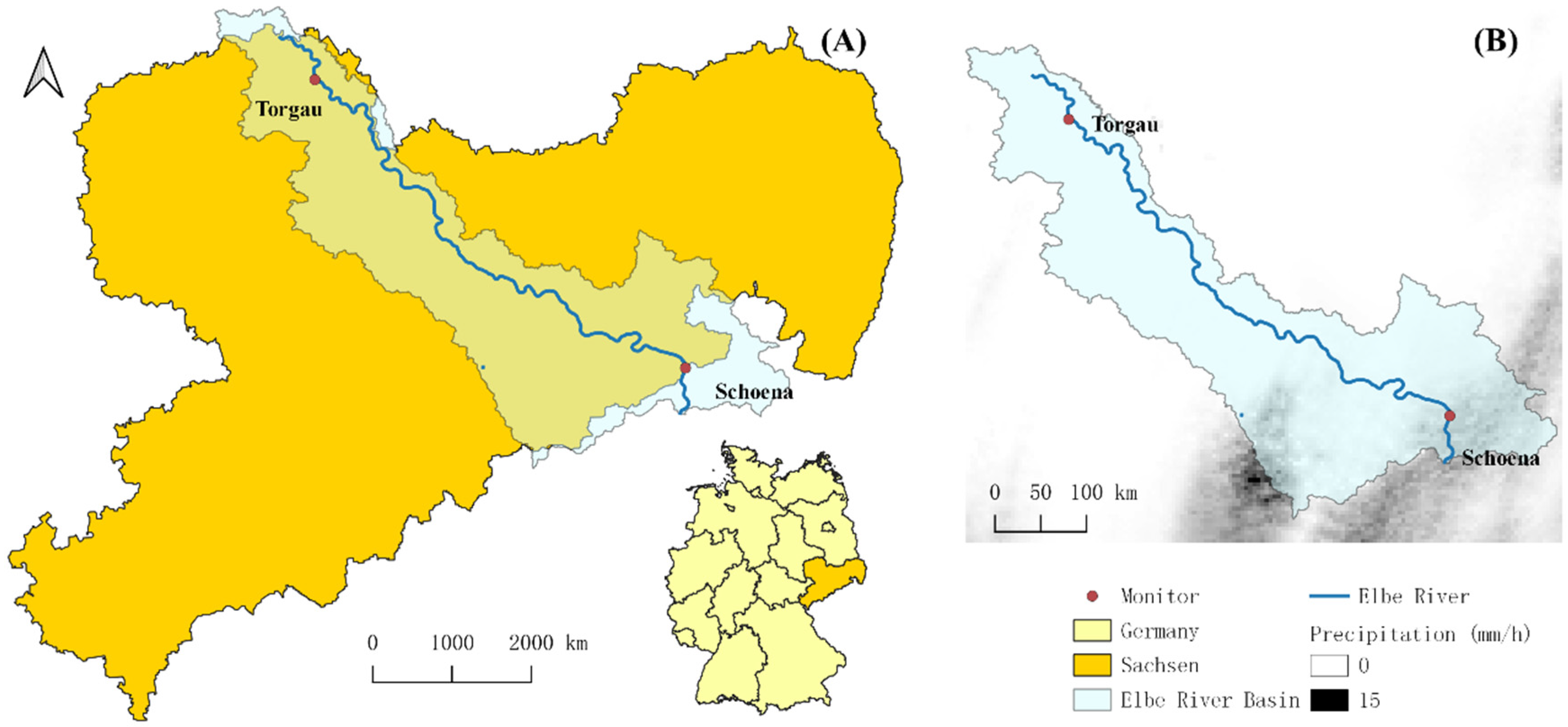
The Elbe is one of Europe’s major rivers, and its total length of it from the Krkonoše Mountains to the North Sea is about 1094 km [48]. The study area is located in the part of the Elbe River basin within Sachsen. As shown in Figure 1A, the Elbe River flows into Sachsen, Germany, from Schoena, and flows out of Sachsen from Torgau.
Figure 1B illustrates an example of the precipitation radar map in this study, according to the information platform UNDINE (http://undine.bafg.de, accessed 29 November 2021), which contains the long-term daily flow data and catchment information of Germany. To study the applicable scope of the model, several recent extreme cases of the Elbe River were collected: January 2011, March and April 2006, and June 2013 for high-water periods; July, August and September 2015, and August and September 2018 for low-water periods [49]. Meanwhile, precipitation radar data of the periods for these extreme cases were extracted from the database of the Deutscher Wetterdienst (DWD, German Meteorological Service, https://cdc.dwd.de/portal/, accessed 30 November 2021). The Elbe River flow data of the periods at Schoena and Torgau were obtained from the Saxon State Office for Environment, Agriculture and Geology (https://www.umwelt.sachsen.de/umwelt/46037.htm, accessed on 30 November 2021).
2.2. Convolutional Neural Network (CNN)
The CNN was introduced for object recognition in digital image processing [50], with a structure composed of a convolution layer, pooling layer, and fully connected layers. The convolution layer applies a convolution filter to input two-dimensional data to generate a feature map. Different feature maps, generated through different filters, are eventually combined to generate a final output. In general, the convolutional layer needs an activation function to enhance the non-linear signal, and a rectified linear unit (ReLU) is usually employed as the activation function [51]. After the convolution layer, the max-pooling layer is used to extract the invariant features by eliminating the non-maximal values with an efficient convergence rate to achieve the purpose of non-linear down sampling [52]. The fully connected layer, linked to the max-pooling layer, connects a loss function to calculate errors between the observed values and model outputs [53]. The mean squared error (MSE) is used as a loss function in the present study.
2.3. Long Short-Term Memory (LSTM)
The LSTM network is a variation of the recurrent neural network (RNN), which adopts a directed cycle structure that transfers the output of a hidden layer to the same hidden layer to identify features and time series information through the signals of the previous time series [54]. LSTM was introduced by Hochreiter and Schmidhuber [39] to overcome gradient disappearance issues through memory cells. The cell states could be updated by a gating regulation consisting of the following three gates: the input gate determines which information will update the present block state and which new datasets will be included as inputs; the forget gate controls which information should be preserved or discarded; the output gate decides which outputs to generate [55]. The following equations were used in LSTM:
Input gate :
Forget gate :
Output gate :
Cell :
Output vector :
where is the cell state vector, is the input at current step t, is an element-wise non-linear activation function, and and denote the bias and weight matrices, respectively.
2.4. River Flow Simulation
In this study, CNN and LSTM network were combined to predict the river flow. The two-dimensional data consisted of rainfall radar images with dimensions of 143 × 159 (1-km resolution), while the upstream flow data were applied as additional information and as single vectors. The upstream flow and rainfall radar time points were calculated based on the time interval with the highest correlation between upstream and downstream flow. The CNN model consisted of one convolutional layer, one max pooling layer, and one flatten layer. The output from the flatten layer was fed into a LSTM model as a one-dimensional feature vector. The outputs from the LSTM layers and the upstream flow were concatenated and transferred to a fully connected layer, thereby generating downstream flow. More detailed descriptions of CNN and LSTM can be found in Section 2.2 and Section 2.3, respectively. In addition, the CNN and LSTM models were implemented using a Keras environment based on Python.3.7
2.5. Performance Evaluation
For the objective function used in hydrologic model performance evaluation, it is desirable to include multiple metrics that could measure different aspects of model performance [56].
One of the most popular objective functions for the performance evaluation of hydrological modelling is the Nash–Sutcliffe efficiency (NSE) [57]. The NSE is defined as follows:
Gupta et al. [58] proposed a new objective function for performance evaluation, the Kling–Gupta efficiency (KGE). The KGE aggregates three components (error, bias, and relative variability of flows) that are decomposed and modified from the NSE as follows:
where is the Pearson correlation coefficient used to evaluate the error, is the bias term used to evaluate the bias, and is a variability term used to measure the relative variability between the flows of observation () and simulation ():
where is the covariance; and are the standard deviation of observation and simulation, respectively; and and denote the mean flows of observation and simulation, respectively.
In addition, the K-fold test was used to verify the generalizability and plausibility of the CNN-LSTM algorithm. K-fold is a technique widely adopted as a model selection criterion, using (K-1) fold data as the training dataset and one-fold as the test dataset after random assignment. It mimicked the application of training and test datasets by repeating the CNN-LSTM algorithm K times.
3. Results
3.1. Flow Time Series
The record of the flow of the Elbe River in Sachsen was highly variable. In the last 15 years, the floods occurred in the Saxon section of the Elbe in 2006, 2011, and 2013. The maximum recorded flows of the Schoena and Torgau in March and April 2006 reached 2720 m3/s and 2870 m3/s, respectively. After that, the flows through Schoena and Torgau in January 2011 reached 2040 m3/s and 2260 m3/s, respectively. In addition, the maximum recorded flows at Schoena and Torgau in June 2013 reached 3710 m3/s and 4040 m3/s, respectively, as the largest flows recorded in recent years. According to research based on statistical data from 1951 to 2006 [59], the high-water recurrence periods in 2006, 2011, and 2013 were ~25, ~8, and ~200 years, respectively. Similarly, the Elbe River experienced two periods of low flows in 2015 and 2018. In July, August, and September 2015, Schoena and Torgau recorded minimum flows of 75.8 m3/s and 89 m3/s, respectively. Moreover, in August and September 2018, Schoena and Torgau recorded minimum water flows of 70.6 m3/s and 90.1 m3/s, respectively.
3.2. Input Selection
The input attributes of the models were constructed based on the Pearson coefficient. The Pearson coefficient provides information about the correlation between two separate time series from different monitoring stations. The Pearson coefficient ranges between 1 and 0, where values nearer to 1 indicate near perfect correlation and values near to 0 suggest complete anti-correlation. The river takes a certain amount of time to flow from upstream (Schoena) to downstream (Torgau), so the intraday flow data of Torgau and one-day- or two-days-ahead Schoena flow data were compared using the Pearson coefficient. As shown in Figure 2, the Pearson correlation between the Torgau flow data and two-days-ahead Schoena flow data was higher at low flow levels, while the opposite was true at high flow levels. The change in the Pearson coefficient indicated that the velocity of water flow was slower during low-water periods, while the velocity of water flow was faster during periods of high water. For the Elbe River flow in this study, the value of the variation in the Pearson coefficient was 209 m3/s. Therefore, the following training situation was divided into high-water period prediction and low-water prediction based on the flow of Schoena (209 m3/s).
During the low-water period, the downstream flow data at Trogau on a particular day was adopted as the CNN-LSTM model output corresponding to the training input data, including the radar maps of the previous 48 h of hourly rainfall and the upstream flow data for Schoena from two days prior. Similarly, the downstream flows corresponded to training data, consisting of the radar maps of the previous 24 h of hourly rainfall and upstream data from a day earlier during the high-water period.
3.3. Flow Simulation
The performance of all the CNN-LSTM models in terms of river flow prediction during model validation phases were evaluated by several statistical indices, including NSE, KGE, r, and . According to the guidelines of the hydrological model performance evaluation proposed by Moriasi [60], the performance of a hydrological model was regarded as very good if the NSE was more than 0.75. Moreover, a refined version of the KGE was adopted to enable further decomposition of the NSE, which facilitated the analysis of the relative importance of its different components (r, , and ) in the context of the rainfall-runoff model. The performance of the CNN-LSTM model was also evaluated through an inspection of graphical representations of the comparisons. Line and scatter plots also enabled us to gain a better understanding of the fit between the measured and forecasting data.
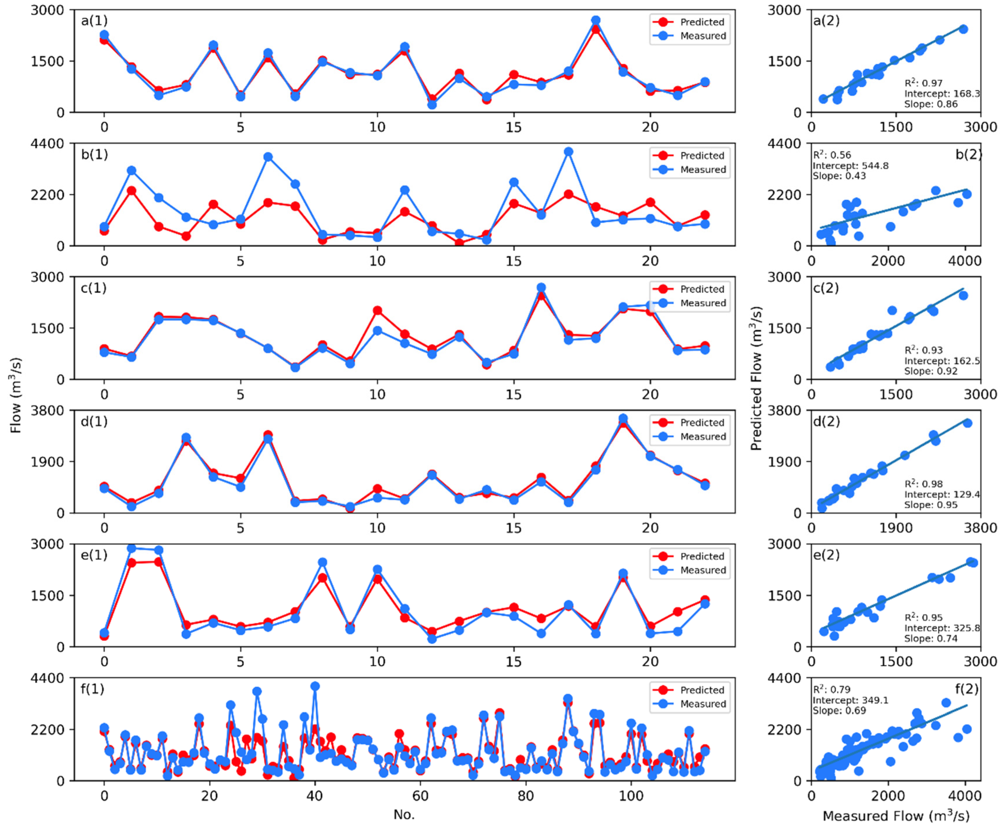
K-fold cross-validated (k = 5) curves were generated from a comparison of the measured and predicted values after the datasets were randomly disrupted according to high-water and low-water periods. According to the high-water period validation shown in Table 1, it was suggested that k3 and k4 have high NSE and KGE values (NSE ≥ 0.9, KGE ≥ 0.9) with a, b, and r close to 1, showing the highest fitting accuracy. The NSE values of k1 and k5 were 0.96 and 0.90, respectively, but the KGE values of the same phases were 0.87 and 0.75, respectively, and their r values were 0.99 and 0.97. The b values were 1.01 and 1.04 which were closer to 1 than those of k3 and k4, but the values were only 0.87 and 0.75, indicating that their fitted fluctuations were slightly inferior to those of K3 and K4. The worst performer, k2, had NSE, KGE, a, b, and c values of 0.46, 0.47, 0.75, 0.58, and 0.80, respectively, all of which were the worst values obtained among all the test results. Collectively, k6 was the combined result of the fivefold test with NSE and KGE values of 0.78, and 0.75, respectively. As shown in Figure 3, the line plot intuitively shows the fitting deviation of the predicted values and the measured values. Figure 3b(1) indicates that the comparison shows an obvious deviation of the prediction effect and almost all the extreme predicted flow values are far lower than the measured values. The scatter plot over the validation phase shows that almost all the points are aligned along the diagonal line of the plots, except the k2 validation phase in the high-water period. However, the magnitude of the coefficient of determination is distinctly sharply worse for k2 validation phase over the whole testing phase—that is, it affected the R2 of the whole testing phase (K6) to 0.79. While k2 attained an R2 of 0.56, the other phases attained an R2 of more than 0.95.
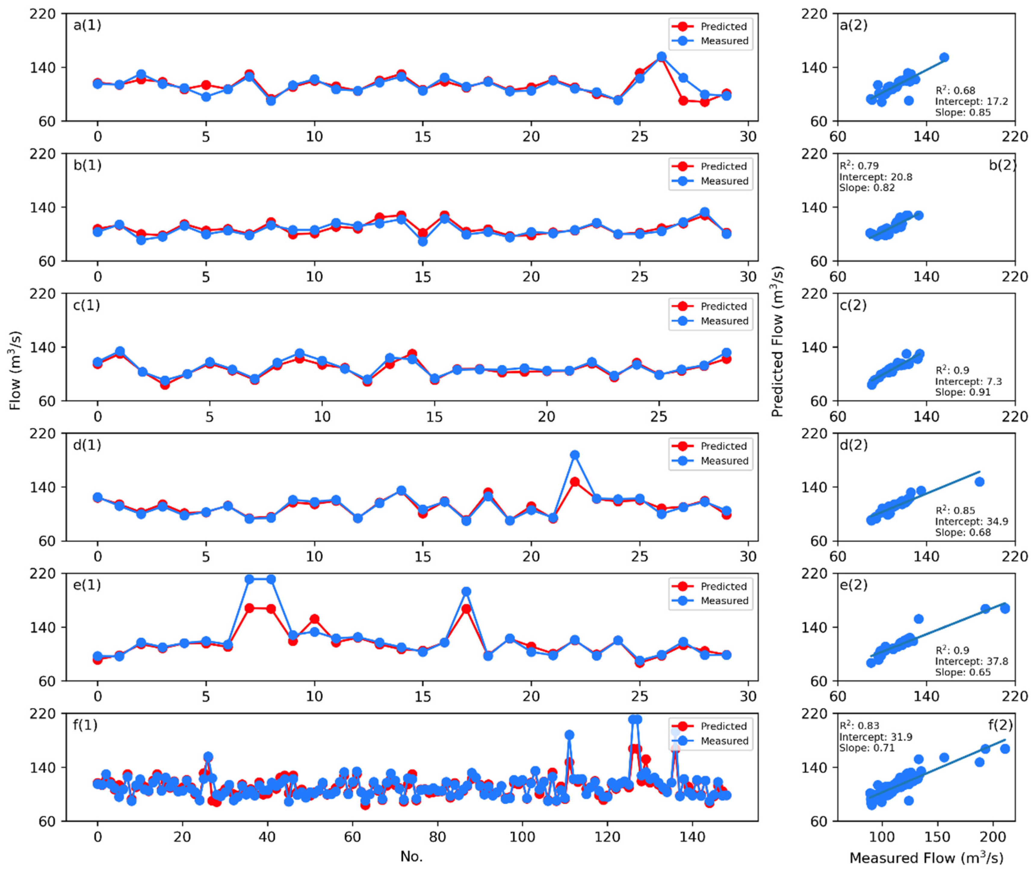
As presented in Table 2, the results of fitting and validation based on the model during the low-water period show that k3 has the highest NSE and KGE values (NSE = 0.86 and KGE = 0.93) with a, b, and r close to 1, showing the highest fitting accuracy. k1 and k2 had higher NSE values than KGE values, while k4 and k5 had higher KGE values than NSE values. It could be seen from r that k4 and k5 had a higher fit while their a-values were only 0.74 and 0.69, indicating the poor performance of the fit with regard to their fluctuations. In all the tests, the b-values were close to 1, indicating that the model for low-water periods was better simulated for the mean value. On balance, k6 was the combined result of the fivefold test, with its NSE and KGE values of 0.81 and 0.76, respectively. As shown in Figure 4, the deviation of the prediction results in the low-water periods is much smaller compared with the high-water periods as the flow during low-water periods is much smaller. The line diagram in Figure 4e(1) shows that the model suggested a large error in predicting the large flow value in the low-water period. The scatter plots show that the magnitude of the coefficients of determination ranged from 0.68 to 0.9.
4. Discussion
In this study, we proposed a method that used CNN to process information on rainfall and LSTM to combine the flow data from the upstream point and time series of the CNN results as inputs into the model. The model computed the spatial relationship between rainfall and runoff through CNN and the temporal connection through LSTM. In this study, the model efficiency (in terms of NSE) was found to be 0.46–0.97 and 0.63–0.86 for high-water and low-water periods, respectively. In a previous study by Sahraei et al. [61], different parametric models (HEC-HMS, HBV-EC, HSPF, WATFLOOD, and Model Wrapper) employed in the Canadian prairies for discharge prediction achieved model NSE of between −0.39 and 0.76. Moreover, the SWAT, XAJ, MLR, BP, and LSTM models were compared by Xu et al. [62] for runoff prediction in the Hun River basins and were found to produce NSE values between 0.35 and 0.79. In a study by Bhagwat and Maity [63], ANN and LS-SVR were employed for one-day-ahead runoff prediction in upper Narmada River basin and achieved a model efficiency (NSE) of between 0.58 and 0.68. In summary, the NSE values achieved in the above studies are less than or equivalent to those obtained using the CNN-LSTM model proposed in this study. If the training data are properly selected, the NSE value of the model could reach more than 0.85 for runoff simulation during high-water or low-water periods (Table 1 and Table 2).
Compared to the parametric model, the advantage of this model was to avoid the complex data collection required by other rainfall-runoff models. For instance, the Hydrological Simulation Program—Fortran (HSPF), an open-source rainfall-runoff model developed by EPA, required rainfall, barometric pressure, air temperature, relative humidity, evaporation, insolation, topographic and land-use data, and the upstream runoff of the study area as the minimum major boundary conditions to run the model [64]. HSPF combined meteorological and geographic data to derive the contribution of rainfall to runoff through physical equations. On the other hand, the CNN-LSTM model required only radar data regarding rainfall and upstream flow data for the study area. The model processed the contribution of rainfall to runoff at the minimum spatial and temporal resolution within each study scale through CNN and LSTM. Although the CNN-LSTM could not show the huge variety of intermediate values in the internal operations, the algorithm continuously adjusted these intermediate values to achieve the best fit, which was equivalent to the calibration phase of the HSPF model that requires human intervention.
Compared to other metric models, the CNN-LSTM could be trained directly on two-dimensional rainfall radar maps and output the predicted flow downstream. In the early 1990s, artificial neural network (ANN) approaches were introduced for rainfall-runoff modeling [65]. In the context of runoff prediction, ANNs employed flexible data-driven techniques to reflect the complicated non-linear connections between input driving factors (precipitation, upstream flow, etc.) and runoff that were difficult to discover using traditional rainfall-runoff modeling approaches. The adjustment of weights and biases in the ANN model corresponded to the contribution of land use, meteorological conditions, and other boundary conditions to the rainfall-runoff process. Limited by the ANN structure itself, the first step in using ANNs for two-dimensional image problems was to convert the two-dimensional images to one-dimensional vectors before training the model. This had two drawbacks: (1) With an increasing image size, the number of trainable parameters and the demand for computer hardware power increased dramatically; (2) ANNs could not capture the sequence information that is required to process sequence data from the input data. Therefore, 2D rainfall radar maps were processed by CNN, and sequence information was processed by LSTM to overcome these two drawbacks in this study.
In addition, the use of models was restricted and their prediction effectiveness for data other than training data is greatly reduced by machine learning [66]. For model prediction of runoff, the accuracy with regard to extreme values was sharply reduced if the trained dataset excludes data obtained under these extreme conditions [67]. Among all the recorded data for flow in Trogau, there were four recorded moments over 3000 m3/s. However, three of them (including two maximum cases) were included in the k2 validation set. Therefore, the training data of k2 were not assigned to most of the extreme values, resulting in poor learning during the training process and a lack of training for high-water value output. In summary, a lack of full scope coverage in the training data could result in low prediction values for some high-water periods during the validation phase, leading to poor prediction results. Therefore, the CNN-LSTM model is particularly important for the selection of input data scope coverage.
In the future, the occurrence of extremes should, on the one hand, be recorded in time and the model should be updated for training. On the other hand, as computer power increases, the use of machine learning models for predicting larger study areas with more rainfall data could be attempted.
5. Conclusions
In this study, the CNN-LSTM model was proposed for river downstream flow prediction. The Elbe River basin in Sachsen, Germany, was selected as the study area, and three high-water cases and two low-water cases were selected as the study period. The performance of models was assessed by KGE and NSE through fivefold validation. The rainfall radar map of the area and the upstream flow were utilized as inputs to the models. The CNN-LSTM model achieved good results in discharge prediction for high-water periods (KGE = 0.75, NSE = 0.78) and low-water periods (KGE = 0.76, NSE = 0.81) with the integrated evaluation of all fold validation sets. However, the CNN-LSTM model underestimated the extreme flows when the one-fold training dataset missed these extreme values (KGE = 0.47, NSE = 0.46), while the other folds performed well (KGE > 0.75, NSE > 0.90) for the high-water period. Therefore, we found that the CNN-LSTM model needs optimized input datasets to achieve better prediction performance. In summary, this study demonstrated the successful application of the CNN-LSTM model in predicting river flow based on two-dimensional rainfall data. This approach could be applied to other river basins with historical rainfall radar data and recorded river flow data. This model will be useful for estimating water availability and flood alerts for river basin management.
Author Contributions
P.L.: Data Curation, Software, Writing; J.Z.: Writing; P.K.: Conceptualization. All authors have read and agreed to the published version of the manuscript.
Funding
This research was funded by the China Scholarship Council (CSC) grant number [201908080087].
Institutional Review Board Statement
Not applicable.
Informed Consent Statement
Not applicable.
Data Availability Statement
Numerical results reported in this paper maybe shared by the interested parties if requested. Please contact the author.
Acknowledgments
The authors would like to gratefully thank the Information platform UNDINE, the Deutscher Wetterdienst (DWD, German Meteorological Service) for providing the data and the Saxon State Office for Environment, Agriculture and Geology for measuring the data. This work was jointly supported by the state-sponsored scholarship program provided by the China Scholarship Council (CSC) (No. 201908080087).
Conflicts of Interest
The authors declare no conflict of interest.
References
- Sitterson, J.; Knightes, C.; Parmar, R.; Wolfe, K.; Avant, B. An Overview of Rainfall-Runoff Model Types. 2018, p. 41. Available online: https://scholarsarchive.byu.edu/iemssconference/2018/Stream-C/41/ (accessed on 5 December 2021).
- Mulvaney, T.J. On the Use of Self-Registering Rain and Flood Gauges in Making Observations of the Relations of Rainfall and Flood Discharges in a given Catchment. Proc. Inst. Civ. Eng. Ireland. 1851, 4, 19–31. [Google Scholar]
- Freeze, R.A.; Harlan, R.L. Blueprint for a Physically-Based, Digitally-Simulated Hydrologic Response Model. J. Hydrol. 1969, 9, 237–258. [Google Scholar] [CrossRef]
- Dzubakova, K. Rainfall-Runoff Modelling: Its Development, Classification and Possible Applications. Acta Geogr. Univ. Comenianae. 2010, 54, 173–181. [Google Scholar]
- O’connell, P.E.; Nash, J.E.; Farrell, J.P. River Flow Forecasting through Conceptual Models Part II-The Brosna Catchment at Ferbane. J. Hydrol. 1970, 10, 317–329. [Google Scholar] [CrossRef]
- Porter, J.W.; McMahon, T.A. Application of a Catchment Model in Southeastern Australia. J. Hydrol. 1975, 24, 121–134. [Google Scholar] [CrossRef]
- Burnash, R.J.C.; Ferral, R.L.; McGuire, R.A. A Generalized Streamflow Simulation System: Conceptual Modeling for Digital Computers; US Department of Commerce: Washington, DC, USA; National Weather Service: Silver Spring, MD, USA; State of California, Department of Water Resources: Sacramento, CA, USA, 1973. [Google Scholar]
- Chiew, F.H.S.; McMahon, T.A. Improved modelling of the groundwater processes in MODHYDROLOG. In Proceedings of the Hydrology and Water Resources Symposium, Perth, Australia, 2–4 October 1991; pp. 492–497. [Google Scholar]
- Zhao, R.J.; Liu, X.R. The Xinanjiang Model. In Computer Models of Watershed Hydrology; Water Resources Publication: Littleton, CO, USA, 1995; pp. 215–232. [Google Scholar]
- Chiew, F.H.S.; Peel, M.C.; Western, A.W. Application and Testing of the Simple Rainfall-Runoff Model SIMHYD. In Mathematical Models of Small Watershed Hydrology and Applications; Water Resources Publication: Littleton, CO, USA, 2002; pp. 335–367. [Google Scholar]
- Refshaard, J.C.; Storm, B. MIKE SHE. In Computer Models of Watershed Hydrology; Water Resources Publication: Littleton, CO, USA, 1995; pp. 809–846. [Google Scholar]
- Donigian, A.S., Jr.; Bicknell, B.R.; Imhoff, J.C. Hydrological Simulation Program-Fortran (HSPF). Comput. Models Watershed Hydrol. 1995, 395–442. [Google Scholar]
- Brunner, G.W. HEC-RAS River Analysis System. Hydraulic Reference Manual. Version 1.0.; Hydrologic Engineering Center: Davis, CA, USA, 1995. [Google Scholar]
- Beven, K.; Lamb, R.; Quinn, P.; Romanowicz, R.; Freer, J. TOPMODEL. Computer Models of Watershed Hydrology; Singh, V.P., Ed.; Water Resources Publication: Littleton, CO, USA, 1995; pp. 627–668. [Google Scholar]
- Wood, E.F.; Roundy, J.K.; Troy, T.J.; van Beek, L.P.H.; Bierkens, M.F.P.; Blyth, E.; de Roo, A.; Döll, P.; Ek, M.; Famiglietti, J. Hyperresolution Global Land Surface Modeling: Meeting a Grand Challenge for Monitoring Earth’s Terrestrial Water. Water Resour. Research. 2011, 47, W05301. [Google Scholar] [CrossRef]
- Ahmed, A.N.; Othman, F.B.; Afan, H.A.; Ibrahim, R.K.; Fai, C.M.; Hossain, M.S.; Ehteram, M.; Elshafie, A. Machine Learning Methods for Better Water Quality Prediction. J. Hydrol. 2019, 578, 124084. [Google Scholar] [CrossRef]
- Clark, M.P.; Bierkens, M.F.P.; Samaniego, L.; Woods, R.A.; Uijlenhoet, R.; Bennett, K.E.; Pauwels, V.; Cai, X.; Wood, A.W.; Peters-Lidard, C.D. The Evolution of Process-Based Hydrologic Models: Historical Challenges and the Collective Quest for Physical Realism. Hydrol. Earth Syst. Sci. 2017, 21, 3427–3440. [Google Scholar] [CrossRef] [Green Version]
- Aziz, K.; Rahman, A.; Fang, G.; Shrestha, S. Application of Artificial Neural Networks in Regional Flood Frequency Analysis: A Case Study for Australia. Stoch. Environ. Res. Risk Assess. 2014, 28, 541–554. [Google Scholar] [CrossRef]
- Kişi, Ö. Streamflow Forecasting Using Different Artificial Neural Network Algorithms. J. Hydrol. Eng. 2007, 12, 532–539. [Google Scholar] [CrossRef]
- Sarle, W.S. Neural Networks and Statistical Models. In Proceedings of the Nineteenth Annual SAS Users Groups International Conference, Cary, NC, USA, 1994, 10–13 April 1994; SAS Institute: Cary, NC, USA; pp. 1538–1550. [Google Scholar]
- Shamseldin, A.Y. Application of a Neural Network Technique to Rainfall-Runoff Modelling. J. Hydrol. 1997, 199, 272–294. [Google Scholar] [CrossRef]
- Rosenblatt, F. The Perceptron: A Probabilistic Model for Information Storage and Organization in the Brain. Psychol. Rev. 1958, 65, 386–408. [Google Scholar] [CrossRef] [PubMed] [Green Version]
- Tu, J.V. Advantages and Disadvantages of Using Artificial Neural Networks versus Logistic Regression for Predicting Medical Outcomes. J. Clin. Epidemiol. 1996, 49, 1225–1231. [Google Scholar] [CrossRef]
- Bray, M.; Han, D. Identification of Support Vector Machines for Runoff Modelling. J. Hydroinformatics 2004, 6, 265–280. [Google Scholar] [CrossRef] [Green Version]
- Sivapragasam, C.; Liong, S.Y.; Pasha, M.F.K. Rainfall and Runoff Forecasting with SSA-SVM Approach. J. Hydroinformatics 2001, 3, 141–152. [Google Scholar] [CrossRef] [Green Version]
- Tehrany, M.S.; Pradhan, B.; Mansor, S.; Ahmad, N. Flood Susceptibility Assessment Using GIS-Based Support Vector Machine Model with Different Kernel Types. Catena 2015, 125, 91–101. [Google Scholar] [CrossRef]
- Hosseini, S.M.; Mahjouri, N. Integrating Support Vector Regression and a Geomorphologic Artificial Neural Network for Daily Rainfall-Runoff Modeling. Appl. Soft Comput. 2016, 38, 329–345. [Google Scholar] [CrossRef]
- Behzad, M.; Asghari, K.; Eazi, M.; Palhang, M. Generalization Performance of Support Vector Machines and Neural Networks in Runoff Modeling. Expert Syst. Appl. 2009, 36, 7624–7629. [Google Scholar] [CrossRef]
- Suykens, J.A.K.; de Brabanter, J.; Lukas, L.; Vandewalle, J. Weighted Least Squares Support Vector Machines: Robustness and Sparse Approximation. Neurocomputing 2002, 48, 85–105. [Google Scholar] [CrossRef]
- Schoppa, L.; Disse, M.; Bachmair, S. Evaluating the Performance of Random Forest for Large-Scale Flood Discharge Simulation. J. Hydrol. 2020, 590, 125531. [Google Scholar] [CrossRef]
- Wang, Z.; Lai, C.; Chen, X.; Yang, B.; Zhao, S.; Bai, X. Flood Hazard Risk Assessment Model Based on Random Forest. J. Hydrol. 2015, 527, 1130–1141. [Google Scholar] [CrossRef]
- Rodriguez-Galiano, V.; Mendes, M.P.; Garcia-Soldado, M.J.; Chica-Olmo, M.; Ribeiro, L. Predictive Modeling of Groundwater Nitrate Pollution Using Random Forest and Multisource Variables Related to Intrinsic and Specific Vulnerability: A Case Study in an Agricultural Setting (Southern Spain). Sci. Total Environ. 2014, 476–477, 189–206. [Google Scholar] [CrossRef] [PubMed]
- Zakariah, M. Classification of Large Datasets Using Random Forest Algorithm in Various Applications: Survey. Int. J. Eng. Innov. Technol. 2014, 3, 189–198. [Google Scholar]
- Rumelhart, D.E.; Hinton, G.E.; Williams, R.J. Learning Representations by Back-Propagating Errors. Nature 1986, 323, 533–536. [Google Scholar] [CrossRef]
- Lin Hsu, K.; Gupta, H.V.; Sorooshian, S. Application of a Recurrent Neural Network to Rainfall-Runoff Modeling. In Proceedings of the 1997 24th Annual Water Resources Planning and Management Conference; Houston, TX, USA, 6–9 April 1997. [Google Scholar]
- Kumar, D.N.; Raju, K.S.; Sathish, T. River Flow Forecasting Using Recurrent Neural Networks. Water Resour. Manag. 2004, 18, 143–161. [Google Scholar] [CrossRef]
- Han, H.; Choi, C.; Jung, J.; Kim, H.S. Deep Learning with Long Short Term Memory Based Sequence-to-Sequence Model for Rainfall-Runoff Simulation. Water 2021, 13, 437. [Google Scholar] [CrossRef]
- Adnan, R.M.; Zounemat-Kermani, M.; Kuriqi, A.; Kisi, O. Machine Learning Method in Prediction Streamflow Considering Periodicity Component; Springer: Singapore, 2021; pp. 383–403. [Google Scholar] [CrossRef]
- Hochreiter, S.; Schmidhuber, J. Long Short-Term Memory. Neural Comput. 1997, 9, 1735–1780. [Google Scholar] [CrossRef]
- Dong, L.; Zhang, J. Predicting Polycyclic Aromatic Hydrocarbons in Surface Water by a Multiscale Feature Extraction-Based Deep Learning Approach. Sci. Total Environ. 2021, 799, 149509. [Google Scholar] [CrossRef]
- Kratzert, F.; Klotz, D.; Brenner, C.; Schulz, K.; Herrnegger, M. Rainfall-Runoff Modelling Using Long Short-Term Memory (LSTM) Networks. Hydrol. Earth Syst. Sci. 2018, 22, 6005–6022. [Google Scholar] [CrossRef] [Green Version]
- Bai, Y.; Bezak, N.; Sapač, K.; Klun, M.; Zhang, J. Short-Term Streamflow Forecasting Using the Feature-Enhanced Regression Model. Water Resour. Manag. 2019, 33, 4783–4797. [Google Scholar] [CrossRef]
- Bai, Y.; Bezak, N.; Zeng, B.; Li, C.; Sapač, K.; Zhang, J. Daily Runoff Forecasting Using a Cascade Long Short-Term Memory Model That Considers Different Variables. Water Resour. Manag. 2021, 35, 1167–1181. [Google Scholar] [CrossRef]
- He, X.; Luo, J.; Zuo, G.; Xie, J. Daily Runoff Forecasting Using a Hybrid Model Based on Variational Mode Decomposition and Deep Neural Networks. Water Resour. Manag. 2019, 33, 1571–1590. [Google Scholar] [CrossRef]
- Barzegar, R.; Aalami, M.T.; Adamowski, J. Coupling a Hybrid CNN-LSTM Deep Learning Model with a Boundary Corrected Maximal Overlap Discrete Wavelet Transform for Multiscale Lake Water Level Forecasting. J. Hydrol. 2021, 598. [Google Scholar] [CrossRef]
- Deng, J.; Dong, W.; Socher, R.; Li, L.-J.; Li, K.; Fei-Fei, L. ImageNet: A Large-Scale Hierarchical Image Database. In Proceedings of the 2009 IEEE Conference on Computer Vision and Pattern Recognition, Miami, FL, USA, 20–25 June 2009; pp. 248–255. [Google Scholar] [CrossRef] [Green Version]
- Baek, S.-S.; Pyo, J.; Chun, J.A. Prediction of Water Level and Water Quality Using a CNN-LSTM Combined Deep Learning Approach. Water 2020, 12, 3399. [Google Scholar] [CrossRef]
- Hesse, C.; Martínková, M.; Möllenkamp, S.; Borowski, I. Baseline Assessment of the Elbe Basin. 2005. Available online: https://www.newater.uni-osnabrueck.de/deliverables/D331_Baseline_Assessment.pdf (accessed on 2 December 2021).
- Schwandt, D.; Hübner, G. Hydrologische Extreme Im Wandel Der Jahrhunderte-Auswahl Und Dokumentation Für Die Informationsplattform Undine. In Forum für Hydrologie und Wasserbewirtschaftung; Technischen Universität Braunschwei: Braunschweig, Germany, 2009; Volume 26, pp. 19–24. [Google Scholar]
- Lawrence, S.; Giles, C.L.; Tsoi, A.C.; Back, A.D. Face Recognition: A Convolutional Neural-Network Approach. IEEE Trans. Neural Netw. 1997, 8, 98–113. [Google Scholar] [CrossRef] [Green Version]
- Krizhevsky, A.; Sutskever, I.; Hinton, G.E. Imagenet Classification with Deep Convolutional Neural Networks. Adv. Neural Inf. Processing Syst. 2012, 25, 1097–1105. [Google Scholar] [CrossRef]
- Nagi, J.; Ducatelle, F.; di Caro, G.A.; Cireşan, D.; Meier, U.; Giusti, A.; Nagi, F.; Schmidhuber, J.; Gambardella, L.M. Max-Pooling Convolutional Neural Networks for Vision-Based Hand Gesture Recognition. In Proceedings of the 2011 IEEE International Conference on Signal and Image Processing Applications, ICSIPA 2011, Kuala Lumpur, Malaysia, 16–18 November 2011; pp. 342–347. [Google Scholar] [CrossRef] [Green Version]
- Wu, J.N. Compression of Fully-Connected Layer in Neural Network by Kronecker Product. In Proceedings of the 8th International Conference on Advanced Computational Intelligence, ICACI 2016, Chiang Mai, Thailand, 14–16 February 2016; pp. 173–179. [Google Scholar] [CrossRef] [Green Version]
- Salehinejad, H.; Sankar, S.; Barfett, J.; Colak, E.; Valaee, S. Recent Advances in Recurrent Neural Networks. arXiv 2017, arXiv:1801.01078. [Google Scholar]
- Graves, A. Long Short-Term Memory. In Supervised Sequence Labelling with Recurrent Neural Networks; Springer: Berlin/Heidelberg, Germany, 2012; pp. 37–45. [Google Scholar]
- Bastidas, L.A.; Hogue, T.S.; Sorooshian, S.; Gupta, H.V.; Shuttleworth, W.J. Parameter Sensitivity Analysis for Different Complexity Land Surface Models Using Multicriteria Methods. J. Geophys. Res. Atmos. 2006, 111, 20101. [Google Scholar] [CrossRef] [Green Version]
- Nash, J.E.; Sutcliffe, J.V. River Flow Forecasting through Conceptual Models Part I—A Discussion of Principles. J. Hydrol. 1970, 10, 282–290. [Google Scholar] [CrossRef]
- Gupta, H.V.; Kling, H.; Yilmaz, K.K.; Martinez, G.F. Decomposition of the Mean Squared Error and NSE Performance Criteria: Implications for Improving Hydrological Modelling. J. Hydrol. 2009, 377, 80–91. [Google Scholar] [CrossRef] [Green Version]
- Bartl, S.; Schümberg, S.; Deutsch, M. Revising Time Series of the Elbe River Discharge for Flood Frequency Determination at Gauge Dresden. Nat. Hazards Earth Syst. Sci. 2009, 9, 1805–1814. [Google Scholar] [CrossRef] [Green Version]
- Moriasi, D.N.; Arnold, J.G.; Liew, M.W.; van Bingner, R.L.; Harmel, R.D.; Veith, T.L. Model Evaluation Guidelines for Systematic Quantification of Accuracy in Watershed Simulations. Trans. ASABE 2007, 50, 885–900. [Google Scholar] [CrossRef]
- Sahraei, S.; Asadzadeh, M.; Unduche, F. Signature-Based Multi-Modelling and Multi-Objective Calibration of Hydrologic Models: Application in Flood Forecasting for Canadian Prairies. J. Hydrol. 2020, 588, 125095. [Google Scholar] [CrossRef]
- Xu, W.; Jiang, Y.; Zhang, X.; Li, Y.; Zhang, R.; Fu, G. Using Long Short-Term Memory Networks for River Flow Prediction. Hydrol. Res. 2020, 51, 1358–1376. [Google Scholar] [CrossRef]
- Bhagwat, P.P.; Maity, R. Multistep-Ahead River Flow Prediction Using LS-SVR at Daily Scale. J. Water Resour. Prot. 2012, 4, 528–539. [Google Scholar] [CrossRef] [Green Version]
- Duda, P.B.; Hummel, P.R., Jr.; Imhoff, J.C. BASINS/HSPF: Model Use, Calibration, and Validation. Trans. ASABE 2012, 55, 1523–1547. [Google Scholar] [CrossRef]
- Daniell, T.M. Neural Networks. Applications in Hydrology and Water Resources Engineering. In Proceedings of the International Hydrology and Water Resource Symposium, Perth, Australia, 30 November–1 December 1991; Institution of Engineers: Perth, Australia, 1991; Volume 3, pp. 797–802. [Google Scholar]
- Peel, M.C.; McMahon, T.A. Historical Development of Rainfall-Runoff Modeling. Wiley Interdiscip. Rev. Water 2020, 7, e1471. [Google Scholar] [CrossRef]
- Imrie, C.E.; Durucan, S.; Korre, A. River Flow Prediction Using Artificial Neural Networks: Generalisation beyond the Calibration Range. J. Hydrol. 2000, 233, 138–153. [Google Scholar] [CrossRef]
Figure 1.
Study area and precipitation radar map. (A) The Elbe River flows into Sachsen, Germany, from Schoena, and flows out of Sachsen from Torgau. (B) An example of the precipitation radar map in this study.
Figure 1.
Study area and precipitation radar map. (A) The Elbe River flows into Sachsen, Germany, from Schoena, and flows out of Sachsen from Torgau. (B) An example of the precipitation radar map in this study.

Figure 2.
The Pearson correlation between downstream (Torgau) flow data and one-day or two-days-ahead upstream (Schoena) flow data.
Figure 2.
The Pearson correlation between downstream (Torgau) flow data and one-day or two-days-ahead upstream (Schoena) flow data.

Figure 3.
Comparison of the predicted values and the measured values in the high-water period. a(1), b(1), c(1), d(1) and e(1) are the predicted and measured values for k1 to k5 folds, respectively, and f(1) is the predicted and measured values for all validation sets. a(2), b(2), c(2), d(2) and e(2) are the scatter plots of the predicted and measured values for k1 to k5 folds, respectively, and f(2) is the scatter plot for all validation sets from k1 to k5.

Figure 4.
Comparison of the predicted values and the measured values in the low-water period. a(1), b(1), c(1), d(1) and e(1) are the predicted and measured values for k1 to k5 folds, respectively, and f(1) is the predicted and measured values for all validation sets. a(2), b(2), c(2), d(2) and e(2) are the scatter plots of the predicted and measured values for k1 to k5 folds, respectively, and f(2) is the scatter plot for all validation sets from k1 to k5.


Table 1.
Evaluation of high-water period.
| R2 | NSE | KGE | r | |||
|---|---|---|---|---|---|---|
| k1 | 0.96 | 0.96 | 0.87 | 0.99 | 0.87 | 1.01 |
| k2 | 0.46 | 0.46 | 0.47 | 0.75 | 0.58 | 0.80 |
| k3 | 0.92 | 0.92 | 0.92 | 0.97 | 0.95 | 1.05 |
| k4 | 0.97 | 0.97 | 0.92 | 0.99 | 0.96 | 1.06 |
| k5 | 0.90 | 0.90 | 0.75 | 0.97 | 0.76 | 1.05 |
| k6 | 0.78 | 0.78 | 0.75 | 0.89 | 0.78 | 0.98 |
Table 2.
Evaluation of low-water period.
| R2 | NSE | KGE | r | |||
|---|---|---|---|---|---|---|
| k1 | 0.63 | 0.63 | 0.82 | 0.82 | 1.03 | 1.00 |
| k2 | 0.76 | 0.76 | 0.86 | 0.89 | 0.93 | 1.02 |
| k3 | 0.86 | 0.86 | 0.93 | 0.95 | 0.96 | 0.98 |
| k4 | 0.81 | 0.81 | 0.73 | 0.92 | 0.74 | 0.99 |
| k5 | 0.82 | 0.82 | 0.68 | 0.95 | 0.69 | 0.97 |
| k6 | 0.81 | 0.81 | 0.76 | 0.91 | 0.77 | 0.99 |
Publisher’s Note: MDPI stays neutral with regard to jurisdictional claims in published maps and institutional affiliations. |
© 2022 by the authors. Licensee MDPI, Basel, Switzerland. This article is an open access article distributed under the terms and conditions of the Creative Commons Attribution (CC BY) license (https://creativecommons.org/licenses/by/4.0/).
Share and Cite
MDPI and ACS Style
Li, P.; Zhang, J.; Krebs, P. Prediction of Flow Based on a CNN-LSTM Combined Deep Learning Approach. Water 2022, 14, 993. https://doi.org/10.3390/w14060993
AMA Style
Li P, Zhang J, Krebs P. Prediction of Flow Based on a CNN-LSTM Combined Deep Learning Approach. Water. 2022; 14(6):993. https://doi.org/10.3390/w14060993
Chicago/Turabian StyleLi, Peifeng, Jin Zhang, and Peter Krebs. 2022. "Prediction of Flow Based on a CNN-LSTM Combined Deep Learning Approach" Water 14, no. 6: 993. https://doi.org/10.3390/w14060993
Note that from the first issue of 2016, this journal uses article numbers instead of page numbers. See further details here.