
Study on the Decoupling Relationship and Rebound Effect between Agricultural Economic Growth and Water Footprint: A Case of Yangling Agricultural Demonstration Zone, China


School of Economics and Finance, Xi’an Jiaotong University, Xi’an 710061, China
Water 2022, 14(6), 991; https://doi.org/10.3390/w14060991
Submission received: 19 December 2021
/
Revised: 15 March 2022
/
Accepted: 17 March 2022
/
Published: 21 March 2022
(This article belongs to the Section Water Use and Scarcity)
Abstract
:The coordinated development of the economy, water resources, and environment is key to the concept of sustainable development. In this study, in respect to the water footprint, it calculated the water resource input and sewage dilution for the Yangling Agricultural Demonstration Area during the agricultural economic growth period from 1999 to 2019. This study also established the Tapio decoupling analysis model on this basis to study the decoupling relationship between economic growth and the water resource environment, as well as its evolution law. A residual free-complete decomposition model was introduced to analyze the influence of the water resource input and sewage dilution on the agricultural economic growth in the Yangling Demonstration Area and its transmission mechanism. The results showed the following: (1) the economic growth and the blue and green water footprints of the Yangling Demonstration Area were decoupled from one another from 1999 to 2019, and the degree of decoupling between economic growth and the grey-water footprint was poor, indicating that economic growth had a more obvious promotion effect on the reduction of water resource consumption, and the pressure on the water environment was increased year by year; (2) the main factor affecting the reduction of water resource consumption in the Yangling Demonstration Area was the effect of technology, and this was greater than the effect of water resource consumption increments resulting from the expansion of the economic scale; (3) the progress of environmental governance technology was the main reason for the decrease in the grey-water footprint in the Yangling Demonstration Area. To improve the quality of our economic development, the pattern of economic development should be transformed to regulate economic growth and expand the scale, reducing water consumption, improving pollutant emission control technology, and making full use of water resources to provide evidence for a reasonable water resource management policy.
1. Introduction
Water resources are important for maintaining the sustainable and healthy development of national economies and societies [1]. Alleviating the pressure on water resources and the environment in the process of social and economic development has become the focus of governments’ decision making and international cooperation agreements. With the continuous and rapid growth of China’s economy, problems such as the conflict between supply and demand for water resources, unsuitable water use structures, and environmental pollution have become important factors affecting the healthy development of China’s economy and society [2,3,4,5]. According to statistics, China’s total water consumption increased from 5590 × 108 m3 in 1999 to 6021 × 108 m3 in 2019, of which agricultural water accounts for 61%. At the same time, wastewater discharge increased from 392 × 108 m3 in 1999 to 802 × 108 m3 in 2019. A forward-looking strategy analysis report entitled “2017–2022 China rural sewage treatment industry development prospects and investment” showed that in China, rural water pollution has become a main cause of the deterioration of the water environment, seriously affecting the rural ecological environment, farmers’ health and safety, and agricultural products. In 2019, China’s rural production, operation, and living consumption of sewage emissions was nearly three million tons, and sewage emissions from 1999 to 2019 reached a growth rate of more than 10% [6]. China’s economic development is strongly dependent on water resources. In the next 10–20 years, water resource consumption and the water environment will become bottlenecks restricting China’s economic and social development [7]. Therefore, it is important to analyze the situation in relation to regional water resource utilization and evaluate the coordination between economic growth and the water resource environment in China in order to solve the current problems and to realize the sustainable utilization of water resources and high-quality economic development.
The water footprint theory, proposed by Tony Allen and Hoekstra et al., provides a new perspective for water resource evaluation [8,9]. A “water footprint” is the total amount of water resources needed for the products and services consumed by a country, region, or individual within a certain period of time. It can be used to analyze the self-carrying capacity and external dependence of regional water resources, contributing to a comprehensive and scientific understanding of the water resource environment [10,11]. Domestic and foreign scholars have studied the water footprint from many different angles, including area [12], industry [13], products [14], water footprint calculation, time and space differences, the influencing factors of the water footprint, the water footprint, agricultural products, animal product structure, the relationship between consumption patterns and the water footprint, and ecological compensation [15,16,17,18]. Sun et al. used the Gini coefficient, the Thiel index, and exploratory spatial data analysis methods to analyze the spatial variation rule and spatial division of China’s interprovincial water footprint intensity. The distribution pattern has also been studied [19]. Zhao et al. based their study on the spatial econometric convergence model to analyze China’s provincial labor average GDP. The spatial autocorrelation of water footprint intensity in China’s provinces was further discussed [20]. Lei et al. constructed a water footprint model and a water footprint intensity model, measuring the water footprint and water footprint intensity for the main provinces in China from 2004 to 2013. They compared the strength of the water footprints based on the exploratory spatial data analysis (ESDA) method, using Moran’s I coefficient and the local spatial auto-correlation analysis (LISA) index of the regional water footprint intensity for global and local autocorrelation analysis [21]. Based on the water footprint theory, Zhang et al. calculated the water footprint intensity of 31 provinces and cities in China from 2002 to 2014 and used the spatial measurement method to explore the spatiotemporal pattern change characteristics of China’s water footprint intensity. The results showed a peak for the spatial agglomeration of China’s water footprint intensity has a peak [22].
China’s rapid agricultural modernization process has been accompanied by the continuous growth of rural economic aggregates, rural water resources, and environmental pressure, but the quantitative relationship between the two and the internal mechanism between them is not completely clear. The relationship between water resources and economic growth is very close. The mismatch between water resources and economic development can seriously restrict economic growth [23,24,25]. Zhang et al. studied the matching relationship between water resources and economic growth nationwide from the perspectives of water resources, distribution, and allocation, and found that the matching relationship between economic factors and water resources in China was indeed poor. They also explained the main regions that affected the matching situation [26,27]. Meng Yu et al. analyzed the matching situation for water resource supply and demand in Henan Province based on the matching relationship between the water resource quantity and GDP of various cities [28]. To study the relationship between water resources and the economy, the existing literature has generally adopted the Gini coefficient method, the imbalance index method, the water use matching index, and other methods. In other literature, the water footprint calculation model VAR and co-integration models have been adopted to study the correlation between water resources and economic growth. Some have also introduced the Theil index into the matching research in relation to water resources and economic development [29,30,31,32,33]. Generally speaking, with rapid economic development and continuous population growth, there will inevitably be a greater demand for water resources. Consumed water will eventually be returned to the environment in the form of untreated wastewater, increasing the local environmental load. In order to curb this extensive growth mode, it is necessary to “decouple” the environmental pressure on water resources from economic growth, thus saving water and reducing waste [34]. With the extensive application of the decoupling theory and its methods in the field of resources and the environment, many scholars have studied the utilization of water resources and their relationship with the economy. Wu constructed a decoupling temporal analysis model to analyze the decoupling situation in relation to water resource consumption and economic development in China from 1953 to 2010 [35]. Pan et al. and Yang et al. analyzed the decoupling situation for water resource consumption and coordinated economic development in Hubei and Jiangxi provinces, respectively [36]. To a certain extent, these studies revealed the level of economic development and consumption patterns associated with water resource utilization for an entire national or provincial administrative area (such as water or waste emissions from the decoupling analysis), but there is very little research in respect of input and output for studying the regional economic growth and water environmental pressure decoupling relationship. Furthermore, existing studies have ignored the effects of economic growth on water resource consumption and wastewater discharge. For a long time, it has been believed that water resource consumption and sewage discharge could be reduced by improving technical efficiency, thus alleviating the pressure on water resources and the environment. Although the effects of technological progress are obvious, total water consumption and wastewater discharge are still increasing in most countries. This is because technological progress leading to improvements in the efficiency of water use can increase the use of water resources, while economic growth can, at the same time, produce new requirements for resource consumption. This leads to a further increase in wastewater emissions, which is partially offset by saving resources and produces the “rebound effect” [37,38]. The objective of this study is to assess water resource pollution and influence factors by applying the methodological framework that handles these limitations. Hence, this study used the blue and green water footprints of agricultural water resources in the process of economic growth as the input index, the grey water footprint in the process of economic growth as the output index, and the Tapio decoupling theory of the area in 1999–2019 to calculate the decoupling of the economic growth and water footprint and the decoupling index. There is currently no complete residual decomposition model that uses economic growth for the blue and green water footprint or the rebound effect of grey water decomposition. Compared to traditional models, the water footprint model can more accurately reflect the input and output of water resources. On this basis, the decoupling and decomposition models were combined to explore the interaction between water resources and the economy. This study was to provide a scientific basis for the formulation and implementation of sustainable development policies for the efficient utilization of water resources.
2. Materials and Methods
2.1. Agricultural Blue and Green Water Footprint
The calculation formula [39,40] for the crop production green water footprint is as follows:
where is the crop production green water footprint (m3/kg), is the crop growth period of green water consumption (m3/hm2), is the crop yield per unit area (kg/hm2), 10 is the conversion coefficient, is the crop growth period in days from the planting season to harvest, is the green water demand for crops (mm), is the crop transpiration from effective precipitation in the evaporation (mm), is the total evaporation of transpiration (mm), is the crop coefficient as a reference crop transpiration by evaporation (mm/d), and is the month of effective rainfall (mm).
The calculation formula for the crop production blue water footprint is as follows:
where represents the blue water footprint of crop production (m3/kg), represents the consumption of the blue water in the growing period of crops (m3/hm2), represents crop evapotranspiration from irrigation water (mm), and represents the blue water demand of crops from the planting period to the harvest period (mm). The standard Penman–Montieth formula was used to solve the potential evapotranspiration of the reference object, and the simplified empirical formula SCS method was used to solve the monthly effective precipitation of crops . Since 98% of the water footprint of animal production comes from feed production, in order to avoid double calculation, only the blue and green water footprints of crop production were calculated in this paper, and the formula is as follows:
2.2. Agricultural Grey Water Footprint
In the process of crop growth, there is large-scale application of chemical fertilizers and pesticides, and except for a few residues in the soil that are absorbed and used by crops, most of them enter water bodies with precipitation or irrigation water, causing pollution to surface runoff and underground water bodies. In China, chemical fertilizer application is dominated by N, P, K, and compound fertilizers. Since N fertilizer makes up the highest proportion of chemical fertilizer application, only the grey water footprint of the total N produced by N fertilizer application was considered in the calculation in this paper [41]. The specific calculation formula is as follows:
where represents the grey water footprint of the planting industry (m3); represents the leaching rate of nitrogen fertilizer (10% was selected in this paper) [42]; denotes the application amount of nitrogen fertilizer (kg), and is the standard concentration of pollutant water quality (kg/m3). According to the first level discharge standard in the Comprehensive Wastewater Discharge Standard (GB8978-1996), the standard concentration of the chemical oxygen demand (COD) and ammonia nitrogen are 60 mg/L and 15 mg/L, respectively (in this paper, the standard concentration of total nitrogen was the standard concentration of ammonia nitrogen). denotes the natural background concentration of pollutants in water under environmental water quality standards (kg/m3), usually set to 0.
If the feces, urine, and wastewater produced by livestock and poultry farming are not treated effectively, the quality of surface water and groundwater will deteriorate. In this paper, the feces and urine produced by representative livestock and poultry (pigs, cattle, sheep, and poultry) in the breeding process were selected as the pollution source from the breeding industry, and the grey water footprint of the livestock and poultry industry was calculated according to the quantity of livestock and poultry breeding, the feeding cycle, the content of pollutants in the feces and urine per unit and the rate of loss into the water body. Since the addition of livestock and poultry will result in a double calculation, the year-end stock of cattle and sheep with a rearing cycle greater than or equal to 365 days was used in this study, while that of pigs and poultry with a rearing cycle of less than 365 days was used. Since the total nitrogen (TN) and COD contents in livestock manure and urine pollutants are relatively high, and water can dilute TN and COD at the same time, the largest grey water footprint produced by TN and COD was selected as the grey water footprint for the livestock and poultry breeding industry. The specific calculation formula is as follows:
where represents the grey-water footprint of the livestock and poultry breeding industry (m3); denotes the total TN or COD content (kg) of the livestock and poultry manure in the water body; denotes the maximum allowable concentration of TN or COD in water under environmental water quality standards (kg/m3); denotes the natural background concentration (kg/m3) of TN or COD in water under environmental water quality standards, which is usually set to zero. Meanwhile, is the number for pigs, cattle, sheep and poultry; is the number of breeding; is the feeding cycle (day); is the daily defecation volume (kg/d); is the daily urine volume (kg/d); is the pollutant content of unit feces (kg/t); is the pollutant content of unit urine (kg/t); is the pollutant loss rate of unit feces (%); is the pollutant loss rate of unit urine (%). Since water dilutes the contaminants in both farming and livestock waste, it only needs to take the larger of the two. Through the above calculations of the grey water footprint of the planting industry and livestock and poultry breeding industries, the calculation formula for the grey water footprint of agriculture is as follows:
where is the total agricultural grey-water footprint ().
2.3. Tapio Decoupling Model
“Decoupling” comes from the field of physics, referring to physical quantities that previously had a response relationship that no longer have said relationship [43]. The decoupling index can be used to represent the degree of non-synchronous change between economic growth and resources and the environment, aiming to reflect the uncertain relationship between economic growth, water resource consumption, and water environmental pressure [44]. At present, there are two main decoupling models. The first is the decoupling factor model based on the initial and last values, proposed by the OECD [45]. The second is the Tapio decoupling index model based on elastic change, that is, the relative amount of change and volume change of two indexes under consideration, where the period for the elastic analysis timescale method reflects the decoupling relationship between variables, overcoming the OECD decoupling model in relation to the base period choice, and further improving the objectivity and accuracy of the decoupling measure [46]. Developed on the basis of the OECD decoupling model, the Tapio decoupling model redefines the concept of decoupling using “decoupling elasticity” and subdivides the types of decoupling to construct the decoupling model as follows:
where is the decoupling elasticity; is the water resource consumption or sewage dilution, represented by the blue and green water footprint of the planting industry and the grey water footprint of agriculture, respectively; is the total regional economic output value. According to the different elastic values, the decoupling types can be divided into the following six categories: strong, weak, recession, expansion negative, weak negative, and strong negative decoupling. Strong decoupling means that the more ideal the decoupling of resources, environmental pressure, and economic growth is, the better the coordinated development state of water resources, the environment, and the economy is. Strong negative decoupling means that the less ideal the decoupling of resources and environmental pressure and economic growth is, the worse the coordinated development state of resources (Table 1).
2.4. Derivation Process for Complete Decomposition Model without Residuals
The complete decomposition model is a factor decomposition method that can completely eliminate the influence of residual errors, and has been applied in the fields of energy, the ecological environment, and land resources. For example, Sun used this model to analyze how economic growth affects energy consumption and energy intensity [47]. Based on the factor decomposition model without residual items proposed by Sun, this study built a complete decomposition model for changes in water footprint driven by economic development and decomposed the remaining items according to the principle “jointly caused and equally distributed” [48]. The following is a simple derivation of the model.
Assume, , that variables are co-determined by factors, and . The variable Y amount in a time period is given by the following:
where , are the contributions of the respective changes of factors to the total change of Y; is the contribution of the change of factor synthesis to the total change of Y; is the contribution of the change of factor synthesis to the total change of Y; is the contribution of the change of factor synthesis to the total change of Y; is the amount left over from the fully decomposed model. According to the principle of equal distribution, the complete decomposition model of the system composed of three factors is as follows:
where and are, respectively, the contribution values and the variation of and to Y.
Based on the complete decomposition model, this study has adopted the IPAT model as the research method [49]. In the equation, represents the blue-green (grey) water footprint generated in the process of economic development. denotes the total population; is the GDP per capita; is technology, which can be expressed as blue-green (grey) per unit GDP. The equation can be expressed as follows:
Based on the above formula, the blue-green (grey) water footprint change can be regarded as the influence of population, scale, and technology effects.
It can be seen from the formula that economic aggregate is mainly affected by population (), scale (), and technology () effects. can be represented the total agricultural population, per capita agricultural GDP, and blue-green (grey) water footprint of unit agricultural GDP in the base period, respectively. These are, , respectively, the change in the amount of total agricultural population in the late period relative to the base period, the change in the amount of per capita agricultural GDP, and the change in the amount of blue-green (grey) water footprint per unit agricultural GDP.
2.5. Study Area
The Yangling Demonstration Zone is the first agricultural high-tech industry demonstration zone in China. At the end of 2019, the permanent resident population was 212,300. The terrain of the region is high in the north and west, and low in the south and east. It has a semi-humid and semi-arid climate and is in the warm temperate zone of east Asia. The average annual temperature is 12.9 °C, the average annual precipitation is 635.1 mm, the average annual sunshine duration is 2163.8 h and the total annual solar radiation is 114.86 kcal/cm2. The terrain is flat, with fertile soil that is suitable for wheat, corn, rapeseed, vegetables, apples, and other crops. In the process of modernization of the agricultural economy and the advanced development of the industrial structure, the water resource environment of the Yangling Demonstration Area has faced severe challenges. The development and utilization of groundwater have accounted for approximately 85% of the water resource development and utilization, and the water resource utilization structure is not fit for purpose. In addition, the irrigation mode is backward, and the per capita living water requirement is high. The water quality of the main rivers in Yangling has seriously deteriorated and the rivers have become black and smelly, which has greatly affected people’s productivity and quality of life. The sharp decrease in arable land area, the shortage of water resources, and the increasingly serious ecological damage and environmental pollution have become the major restraining factors for the further development of the Yangling Agricultural Demonstration Zone.
2.6. Data Sources
This study used meteorological data from China’s meteorological data network (http://data.cma.cn/, (accessed on 17 May 2021)), including the monthly average temperature (°C), monthly average highest temperature (°C), monthly mean minimum temperature (°C), monthly average wind speed (m/s), sunshine time (h), monthly average relative humidity (%), average vapor pressure, average monthly precipitation, and various meteorological site longitudes, latitudes, altitudes, elevations, etc. [50].
Crop growth-related data, such as crop coefficients and crop growth stage data, were used as references to the publications Water Demand and Irrigation for Major Crops in China, and Water Demand for Crops and Regional Irrigation Patterns in Shaanxi Province, and standard crop coefficients of 84 crops recommended by FAO-56 [51].
The soil data used were from the FAO Global Database, including the total available soil moisture, maximum rainfall infiltration rate, and maximum water depth [52].
The agricultural products were divided into crop and animal products. The crop products included winter wheat, summer corn, rapeseed, vegetables, fruits, and melons, while the animal products included pork, beef, mutton, poultry, eggs, milk, and aquatic products. The Yangling Demonstration Zone main crop planting area, its main agricultural production, its main crop yield per unit area, the agricultural She-Chun nitrogen quantity from the agricultural population, and the agricultural GDP were taken from the Shaanxi Statistical Yearbook (1999–2019). For the Yangling Demonstration Zone, the Shaanxi Statistical Yearbook uses the numerical average of the sum of the adjacent years for some of the missing years of data. Among these, the GDP data for the Yangling Demonstration Area from 1999 to 2019 were all converted at constant prices in 1999.
3. Results
3.1. Overall Description of E and WF
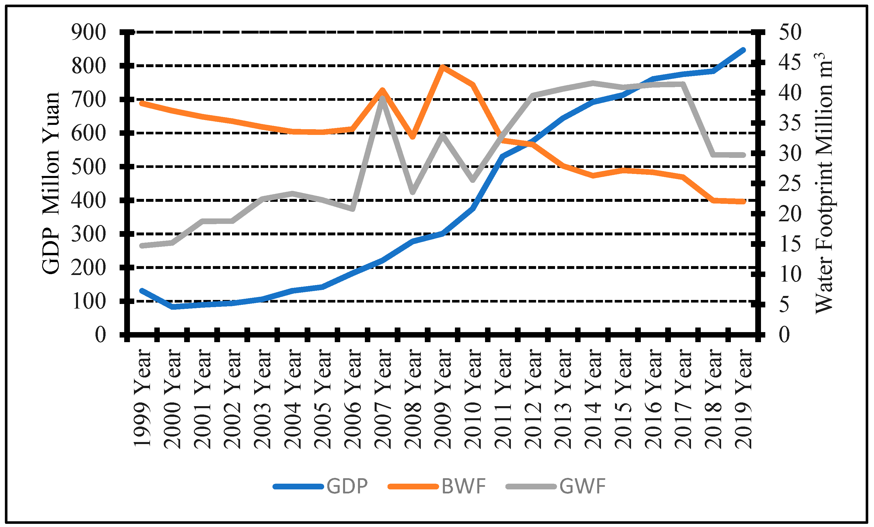
Taking 1999 as the base period, the actual agricultural GDP, and blue and green and grey water footprints of the Yangling Demonstration Zone from 1999 to 2019 were calculated as the economic growth and water footprint. As shown in Figure 1, the real agricultural GDP increased from 131 million yuan in 1999 to 821 million yuan in 2019, representing an average annual growth rate of 26.34%. The blue and green water footprint decreased from 38,246,500 m3 in 1999 to 22,007,800 m3 in 2019, with an average annual decrease of 2.12%. The grey-water footprint increased from 14,725,400 m3 in 1999 to 29,695,800 m3 in 2019, with an average annual growth of 5.09%. During the study period, the water footprint (WF) increased with the increase in agricultural GDP, and the pressure of economic development on the water environment was still high. The blue and green water footprint showed a gentle downward trend, indicating that the dependence of economic growth on water resources has decreased.
3.2. Analysis of the Decoupling Relationship between E and WF
In terms of decoupling measures, the decoupling relationship between agricultural economic growth and the water footprint in the Yangling Demonstration Area from 1999 to 2019 was evaluated by combining the decoupling classification in Formula (11) and Table 1. It can be concluded that strong negative decoupling accounted for 2.5%, weak negative decoupling for 2.5%, expansion negative decoupling for 15%, weak decoupling for 25%, and strong decoupling for 55%. In order to further clarify the relative relationship between agricultural economic growth and water resources and the water environment, the decoupling model was used to analyze the relationship between agricultural economic growth and the blue and green water footprint (water resource consumption) and grey water footprints (water diluted by pollutants) in the Yangling Demonstration Area.
(1) There was a strong decoupling between agricultural economic growth and the blue-green water footprint. As shown in Table 2, the weak negative decoupling state in 2000 expanded in 2009 to negative decoupling with slow economic growth, but the blue and green water footprint greatly increased. Other years were in a weak decoupling state, primarily due to slow economic and resource consumption growth, such as during 2000, when the blue and green water footprint of a growth rate of 3.6% was far more than the GDP growth rate of 35.19%. In 2009, the decoupling state was the most significant, and the elasticity coefficient of the GDP of the blue and green water footprint reached 6.21. During this period, the economic growth rate of the Yangling Demonstration Area slowed down, but the growth rate of the blue and green water footprint increased significantly, at a growth rate of 35.15%, which was much higher than the GDP growth rate of 5.66. This growth can be divided into the following three stages: The period from 2000 to 2009 is the first stage, which is the fluctuation period. In the stage of economic growth, the blue and green water footprint of the Yangling Demonstration Zone experienced “weak negative decoupling-strong decoupling-weak decoupling-expansion negative decoupling”. During this process, the decoupling index also showed a trend of decline before rising and falling. This occurred because, in this period, the traditional extensive mode in the Yangling Demonstration Zone occupied the dominant position (farming, animal husbandry, and the development of rural non-agricultural industries were relatively slow, greatly restricting the development of the rural economy). However, because many large agricultural enterprises in the Yangling Demonstration Area are still in the development mode of high capital consumption, high energy consumption, and low efficiency, they are still highly dependent on water resources, and the relationship between economic development and the blue and green water footprint is always in a state of fluctuation. The period from 2010 to 2019 is the second stage, which was a stable period. During this period, economic growth kept rising, while the blue and green water footprint continued to decline. This is mainly because of the global economic crisis in 2008, during which four trillion yuan was provided by the Chinese government’s bailout plan, and, against the background of a new countryside construction policy, the Yangling Demonstration Zone relied on new technology to develop its rural industry, optimize its rural industrial structure, and promote agricultural modernization, planting, animal husbandry, and aquaculture. In addition, it undertook comprehensive development of non-agricultural industries and, to a certain extent, eliminated the disadvantages of the dual structure between urban and rural areas such as education and healthcare, and the construction of a new rural economy in the Yangling Demonstration Zone became the focus of the policy.
(2) The decoupling relationship between agricultural economic growth and GWF is mainly reflected in the alternating change of expansion negative decoupling, weak decoupling and strong decoupling. In 2005–2006, 2008, 2010, 2015, and 2018–2019, strong decoupling was observed; that is, the economic growth and grey water footprint decreased, indicating that water environmental pressure decreased. In 2002, 2004, 2011, 2013–2014, and 2016–2017, a weak decoupling state was observed; that is, the economic growth and the increase in the grey water footprint, indicating the slow growth of water environmental pressure. The five years of 2001, 2003, 2007, 2009, and 2012 showed negative decoupling of expansion; that is, the grey water footprint increased significantly while the economy grew slowly, indicating a significant increase in the water environmental pressure. Of these, the decoupling index in 2000 was the lowest; that is, the decoupling effect of economic growth and environmental pressure was the least ideal. The growth rate of the grey water footprint was 3.4%, which was much higher than the growth rate of the actual agricultural GDP (35.19%), so there was strong negative decoupling. This can be divided into the following three stages: 2000–2004 is the first stage, alternately showing strong negative decoupling, weak decoupling, and expanding negative decoupling states. Due to the impact of the Asian financial crisis, the agricultural economic growth during this period was relatively slow, and the water consumption was limited, however, farming and animal husbandry pollutant emissions appeared to be a rising trend and the grey water footprint also rose, so economic development and environmental pressure decoupling was poorer. With the development of the rural economy, the consumption of water resources decreased slowly, but the pressure of water environmental pollution increased rapidly. The period from 2005 to 2012 is the second stage. At this stage, economic development accelerated, the consumption of water resources and the water environmental pressure slowly decreased, and the degree of interdependence between the two gradually decreased and fluctuated, demonstrating an alternating process of strong decoupling to expansion and negative decoupling. The period 2013–2019 is the third stage, with economic growth and a relatively stable water environment pressure decoupling state, characterized alternately by strong and weak decoupling states. The Yangling Demonstration Zone was at a time when the transformation of the mode of economic development was strengthened to improve the quality of economic development and reduce the water environment of economic growth in the process of cost-effective scientific development. The grey water footprint appeared to be an obvious turning point in 2015. After years of growth, at this point, it was on the decline because, in April 2016, China signed the Paris agreement. On the eve of the signing, China established a water-saving society for environmental protection, and during the subsequent period, the Yangling Demonstration Zone issued a number of water environmental protection policies, mainly to limit the use of fertilizers and pesticides, which resulted in a significant decline in the quantity of chemical fertilizers. With the in-depth promotion of agricultural modernization and rural revitalization policies, the reduction of agricultural water, soil, fertilizer, and other resources has led to the beginning of a downward trend in the grey water footprint.
3.3. Analysis of the Rebound Effect of the Water Footprint
Using the rebound effect decomposition model constructed in Equations (17)–(19), the population, scale, and technology effects of the blue and green and grey water footprints of the Yangling Demonstration Area from 1999 to 2019 were calculated. The population effect reflects the change in the blue and green water footprint or grey water footprint caused by population growth. The scale effect reflects the change in blue green water footprint or the grey-green water footprint caused by the economic control effect through technical efficiency. In the Yangling Demonstration Zone, however, the period 1999–2019 as a whole indicates a negative effect of technology on the grey water footprint; the technical efficiency of the pollutant emissions decreased, but the amount of sewage dilution continued to rise, indicating that the growth of the population and the expansion of economic scale meant that improvements in technical efficiency brought about by the potential purifying water environment were not fully realized, thus illustrating the rebound effect expansion. The technological effect reflects the change in the blue and green water footprint or grey green water footprint caused by technological progress. According to the rebound effect of the changes in the blue and green water footprint and grey water footprint shown in Table 3, the changes in the blue-green water footprint for the Yangling Demonstration Area showed a rapid downward trend from 1999 to 2019. However, the grey water footprint fluctuated and increased. Population growth and the expansion of economic scale are the main reasons for the increase in the blue and green water footprint and grey water footprint. The Yangling Demonstration Zone is a national agricultural high-tech demonstration area, and its high degree of agricultural modernization and the rapid development of the economy were bound to cause blue and green and grey water footprint increases and stress effects on the ecological environment, as well as tremendous environmental pressure. Therefore, the Yangling Demonstration Zone is presently at a stage of economic development in terms of the blue and green water footprint and the incremental effect of the ash water footprint. Despite the growth in population, the blue and green water footprint and grey water footprint also play a positive role, but the Yangling Demonstration Zone’s agricultural population dropped from 83,634 people in 1999 to 72,000 people by 2019, a fall of 14%, while the real agricultural real GDP increased from 131 million yuan in 1999 to 821 million yuan in 2019, increasing 5.3 times. Agriculture was far higher than the population growth rate of the real GDP; therefore, the blue and green water footprint and grey water footprints of the economic scale effect were higher than the population effect. Another factor affecting the rebound effect is the technical effect. Due to continuous improvements in technical efficiency, both the intensity of the blue and green water footprint and the pollutant discharge intensity were continuously decreased, which inhibited the blue and green water footprint and the grey water footprint. It directly reflects the influence, direction, and contribution of the population, scale, and technology effects on the blue and green and grey water footprints. As can be seen from Table 3, except for 2000 and 2009, the contribution of the scale effect to the blue and green water footprint was all positive, and the contribution was maximal. Except for 2009–2011, the contribution of the population effect to the blue and green water footprint was all positive, but it is small. Except for 2000 and 2009, the contribution of the technology effect to the blue and green water footprint was negative, and the contribution degree was large. As can be seen from Table 3, except for 2009–2011, the contribution of the population effect to the GWF was small, and it showed an obvious growth trend after 2015. Except for 2000, 2009, and 2018, the contribution direction of scale effect on GWF was positive, and the contribution showed a trend of first increasing and then decreasing, reaching a maximum in 2011. Except for 2000–2001, 2007, 2009, and 2012, the contribution direction of the technology effect to the GWF is negative in other years, and the contribution degree is relatively high, which was larger than the scale effect. In the Yangling Demonstration Zone, although during the period 1999–2019, the technical effect on the blue-green water footprint was negative overall, due to the technical efficiency of water saving, agricultural water consumption continued to decline, indicating that, even though there was a growth in population and an expansion of economic scale, the technological progress for the reduction of the water pressure was greater than the population growth and economic expansion, and the incremental effect of the water pressure. There was no rebound effect, and the blue and green water footprint can have a good trend.
4. Discussion and Conclusions
4.1. Conclusions
- (1)
- In the Yangling Demonstration Zone, agriculture from 1999 to 2019 demonstrated real GDP growth at an average annual rate of 26.34%, with the blue and green and grey water footprints showing an average annual growth of 2.12% and 5.09%, respectively. The economic growth and the positive correlation of water resources and water environment, with a negative correlation in the Yangling Demonstration Zone at the same time, suggests the low water, high emissions, and high pollution of the extensive economic development mode.
- (2)
- Through the use of the topic decoupling model, it can be seen that the economic growth and blue and green water footprint of the Yangling Demonstration Area from 1999 to 2019 presented weak decoupling and strong decoupling, respectively, indicating that the economic growth was better without the dependence on water resources. Relative to water resource investment, economic growth, and the decoupling degree of the grey water footprint were lower than the economic growth and the decoupling degree of the blue and green water footprint, indicating that the economic developments to strengthen the water environmental pressure have a more obvious role in promoting. At the same time, the Yangling Demonstration Zone showed that the current focus on research into the water input and output of the neglected environmental pollution source management governance mechanism is not conducive to reducing the pressure on the water environment.
- (3)
- By using the complete decomposition model, an empirical analysis of the blue and green and grey water footprints in the Yangling Demonstration Area showed that the water resource environmental pressure in this area is subject to the expansion of the agricultural economic scale, the promoting effect of the agricultural population, and the inhibiting effect of technological effect. Of these, technological progress is the main reason for the large decrease in the blue and green water footprint in the Yangling Demonstration Area, and this effect is greater than the increased intensity effect for the blue and green water footprint caused by the expansion of economic scale and population growth. The expansion of the agricultural economy is the main reason for the increase in the grey water footprint in the Yangling Demonstration Area.
4.2. Policy Recommendations
This study used the agricultural high-tech Yangling Demonstration Area with a high-degree of agricultural modernization as our research area, analyzing the agricultural economic growth and blue and green water footprint decoupling relationships and exploring the internal mechanisms for these, in order to target specific factors and put forward development countermeasures. To make the research question more targeted, the Yangling Demonstration Zone was used to investigate agricultural economy sustainable development and water environmental pressure to provide a scientific basis for reducing the current “win-win” policy.
- (1)
- Establish a farmland management and nitrogen fertilizer application technology system with a high resource efficiency and reduced input. The utilization rate of fertilizer can be improved by increasing the technical input, popularizing soil testing and formula fertilization technology, optimizing and balancing fertilization, and developing and popularizing new fertilizers, so as to reduce the grey water footprint from the source.
- (2)
- The mode of economic growth and the control of water consumption should be changed so as to achieve the goal of an absolute decoupling of economic growth and the water footprint. To truly achieve sustainable development, it is necessary to optimize the allocation of water resources and regulate crops with high emissions, high pollution, and low income. The spatial and temporal distribution of agricultural land use should be scientifically and rationally planned, and the land use structure should be optimized. In addition, from the perspective of ecological engineering design, setting up an ecological buffer zone and an isolation ditch can effectively reduce the negative impact of the grey water footprint on the economy and the environment.
- (3)
- The economic growth rate should be regulated, and water use efficiency should be improved. Technological progress is slow, and improvements in water use efficiency brought by technological progress are limited. In order to truly achieve efficient water saving and sustainable development, the total agricultural population must be controlled, and at the same time, scientific and technological innovation and management efforts must be further strengthened to reduce water consumption and pollutant discharge, so as to make full use of water resources. The economic growth rates and expansion scales should also be reasonably regulated, so as to limit the unnecessary wastage of water resources.
Funding
This research was funded by the Social Science Major Project of Shaanxi Province (2021ND0378, 2021HZ0933), China Postdoctoral Science Foundation (2021M692655), and the Social Science Foundation of Ministry of Education (21YJC630086).
Institutional Review Board Statement
This study mainly focused on the models and data analysis and did not involve human factors considered dangerous. Therefore, ethical review and approval were waived for this study.
Informed Consent Statement
Not applicable.
Data Availability Statement
Data are available on request due to restrictions, e.g., privacy or ethical. The data presented in this study are available on request from the corresponding author. The data are not publicly available due to the strict management of various data and technical resources within the research teams.
Acknowledgments
I also appreciate the constructive suggestions and comments on the manuscript from the reviewer(s) and editor(s).
Conflicts of Interest
The author declares no conflict of interest.
References
- Zeng, Y.; Hong, H.S.; Cao, W.Z.; Chen, N.; Li, Y.; Huang, Y. Characteristics of nitrogen and phosphorus losses from swine production systems in Jiulong River watershed. Trans. CSAE 2005, 21, 116–120. [Google Scholar]
- Chen, X.W. Environment and China’s rural development. Manag. World 2002, 1, 5–8. [Google Scholar]
- Cohen, A.; Sullivan, C.A. Water and poverty in rural China: Developing an instrument to assess the multiple dimensions of water and poverty. Ecol. Econ. 2010, 69, 999–1099. [Google Scholar] [CrossRef] [Green Version]
- Li, Y.M.; Wang, J.X. Situation, Trend and Its Impacts on Cropping Pattern of Water Shortage in the Rural Areas: Empirical Analysis Based on Ten Provinces’ field Survey in China. J. Nat. Resour. 2009, 24, 200–208. [Google Scholar]
- Liu, Y.; Liu, W.J.; Zhao, Y.W. Fitting analysis of relation of agricultural excessive nitrogen to rural resident consumption in Jiangsu Province. Bull. Soil Water Conserv. 2012, 32, 82–86. [Google Scholar]
- Jiang, X.Y.; Zhao, S. An empirical study on the relationship between economic growth, industrial structure and carbon emissions in Jiangsu Province. J. Nanjing Univ. Financ. Econ. 2020, 2, 16–24. [Google Scholar]
- Hoy, L.; Stelli, S. Water conservation education as a tool to empower water users to reduce water use. Water Sci. Technol. Water Supply 2016, 16, 202–207. [Google Scholar] [CrossRef]
- Mohammadi, H.; Mohammadi, A.M.; Nojavan, S. Factors affecting farmers chemical fertilizers consumption and water pollution in Northeastern Iran. J. Agric. Sci. 2017, 9, 234–241. [Google Scholar]
- Yang, J.; Li, J.Q. Research on the relationship between agricultural economic growth, agricultural structure, and agricultural non-point source pollution in Fujian Province. Chin. J. Eco-Agric. 2020, 28, 1277–1284. [Google Scholar]
- Xu, Z.M.; Long, A.H. The primary study on assessing social water scarcity in China. Acta Geogr. Sin. 2004, 59, 982–988. [Google Scholar]
- Allan, J.A. Fortunately There Are Substitutes for Water Otherwise Our Hydro-Political Futures Would Be Impossible; ODA: London, UK, 1993. [Google Scholar]
- Hoekstra, A.Y. Virtual Water Trade: An Introduction. In Proceedings of the International Expert Meeting on Virtual Water; Value of Water Research Report Series No. 12; IHE: Bunkyo City, Tokyo, 2003. [Google Scholar]
- Hoekstra, A.Y.; Chapagain, A.K.; Mekonnen, M.M.; Aldaya, M.M. The Water Footprint Assessment Manual: Setting the Global Standard; Earth-Scan: London, UK, 2011. [Google Scholar]
- Hoekstra, A.Y. Humanity’s unsustainable environmental footprint. Science 2014, 344, 1114–1117. [Google Scholar] [CrossRef] [PubMed]
- Pellicer, M.F.; Martínez, J.M. Grey water footprint assessment at the river basin level: Accounting method and case study in the Segura River Basin, Spain. Ecol. Indic. 2016, 60, 1173–1183. [Google Scholar] [CrossRef]
- Wu, B.; Zeng, W.H.; Chen, H.H.; Zhao, Y. Grey water footprint combined with ecological network analysis of assessing regional water quality metabolism. J. Clean. Prod. 2015, 112, 3138–3151. [Google Scholar] [CrossRef]
- Nandan, A.; Yadav, B.P.; Baksi, S.; Bose, D. Assessment of water foot-print in paper and pulp industry and its impact on sustainability. World Sci. News 2017, 64, 84–98. [Google Scholar]
- Liu, W.; Antonelli, M.; Liu, X.; Yang, H. Towards improvement of grey Water footprint assessment: With an illustration for global maize Cultivation. J. Clean. Prod. 2017, 147, 1–9. [Google Scholar] [CrossRef]
- Chapagain, A.K.; Hoekstra, A.Y. The blue, green and grey water footprint of rice from production and consumption perspectives. Ecol. Econ. 2011, 70, 749–758. [Google Scholar] [CrossRef]
- Li, Y.; Lu, L.; Tan, Y.; Wang, L.; Shen, M. Decoupling water consumption and environmental impactom textile industry by using water footprint method: A case study in China. Water 2017, 9, 124. [Google Scholar] [CrossRef]
- Feng, K.; Hubacek, K.; Minx, J.; Siu, Y.L.; Chapagain, A.; Yu, Y.; Guan, D.; Barrett, J. Spatially explicit analysis of footprint in the UK. Water 2011, 3, 47–63. [Google Scholar] [CrossRef] [Green Version]
- Sun, C.Z.; Liu, Y.Y.; Chen, L.X.; Zhang, L. The spatial-temporal disparities of water footprints intensity based on Gini Coefficient and Theil Index in China. Acta Ecol. Sin. 2010, 30, 1312–1321. [Google Scholar]
- Zhao, L.S.; Sun, C.Z.; Zou, W. Convergence between economic growth and water footprint intensity at the provincial scale in China. Resour. Sci. 2013, 35, 2224–2231. [Google Scholar]
- Lei, Y.T.; Su, L. Spatial analysis of the regional differences of water footprint intensity in China. Ecol. Econ. 2016, 32, 29–35. [Google Scholar]
- Zhang, L.L.; Shen, J.Y. Temporal and spatial pattern evolution and driving factors analysis of China’s water footprint intensity. Stat. Decis. 2017, 17, 143–147. [Google Scholar]
- Lang, Y.H.; Wang, L.M. The Types of Deficient Resources and the Trend of Supply and Demand. J. Nat. Resour. 2002, 17, 409–414. [Google Scholar]
- Li, X.F.; Zhu, J.Z.; Gu, X.J.; Zhu, J.J. Current situation and control of agricultural non-point source pollution. China Popul. Resour. Environ. 2010, 20, 81–84. [Google Scholar]
- Wen, C.H.; Zhang, D.; Tie, Y. Environmental effects of agricultural non-point source pollution and its coupling impact on new rural construction. Guizhou Soc. Sci. 2008, 4, 91–96. [Google Scholar]
- Zhang, F.; Hu, H.; Zhang, H. The positive analysis on the relationship between agriculture non-point source pollution and economic growth of Jiangsu Province. China Popul. Resour. Environ. 2010, 20, 80–85. [Google Scholar]
- Zhong, M.C. The unreality of environmental Kuznets curves and its impact to sustainable development. China Popul. Resour. Environ. 2005, 15, 1–6. [Google Scholar]
- Peng, W.B.; Tian, Y.H. Empirical research on environmental pollution and economic growth in Hunan Province—Based on impulse response function of VAR model. J. Xiangtan Univ. Philos. Soc. Sci. 2011, 35, 31–35. [Google Scholar]
- Liu, Q.; Hu, X.J. Comparison of the water quality of the surface microlayer and subsurface water in the Guangzhou segment of the Pearl River, China. J. Geogr. Sci. 2014, 24, 475–491. [Google Scholar] [CrossRef]
- Fang, C.L.; Wang, Y.; Fang, J.W. Acomprehensive assessment of urban vulnerability and its spatial differentiation in China. J. Geogr. Sci. 2016, 26, 153–170. [Google Scholar] [CrossRef]
- Yang, Y.; Liu, Y. Spatio-temporal analysis of urbanization and land and water resources efficiency of oasis cities in Tarim River Basin. Acta Geogr. Sin. 2012, 24, 509–525. [Google Scholar] [CrossRef]
- Wang, Z.; Feng, H.J.; Xu, S.Y. Analysis of Water Resource Problem in Chinese Economic Development. Chin. J. Manag. Sci. 2001, 9, 47–56. [Google Scholar]
- Ma, X.H.; Fang, S.H. Water and Growth in an Agricultural Economy. Chin. Rural Econ. 2006, 10, 4–11. [Google Scholar]
- Liu, W.; Xu, R.; Deng, Y.; Lu, W.; Zhou, B.; Zhao, M. Dynamic Relationships, Regional Differences, and Driving Mechanisms between Economic Development and Carbon Emissions from the Farming Industry: Empirical Evidence from Rural China. Int. J. Environ. Res. Public Health 2021, 18, 2257. [Google Scholar] [CrossRef] [PubMed]
- Wang, X.Y.; Han, H.Y. Growth Drag of Water Resources to Agriculture in China. J. Econ. Water Resour. 2008, 5, 1–5. [Google Scholar]
- Liu, Y.; Du, J.; Zhang, J.B. Hypothesis and Validation of the Kuznets Curve of Agricultural Water Use and Economic Growth. Resour. Environ. Yangtze Basin 2008, 17, 594–597. [Google Scholar]
- Yu, F.W. Decoupling Analysis of Food Production and Irrigation Water in China. Chin. Rural Econ. 2008, 10, 34–44. [Google Scholar]
- Fu, Y.; Liu, L.; Yuan, C. Comprehensive evaluation for nitrogen footprint and grey water footprint of agricultural land use system. Trans. Chin. Soc. Agric. Eng. 2016, 32, s312–s319. [Google Scholar]
- Hoekstra, A.Y. Human appropriation of natural capital: A comparison of ecological footprint and virtual water footprint analysis. Ecol. Econ. 2009, 68, 1963–1974. [Google Scholar] [CrossRef] [Green Version]
- Ma, H.; Hou, Y.; Li, S. Decoupling relationship between industrial wastewater discharges and economic growth in regional differentiation of China. China Popul. Resour. Environ. 2017, 27, 185–192. [Google Scholar]
- OECD. Indicators to Measure Decoupling of Environmental Pressure from Economic Growth; OECD: Paris, France, 2002. [Google Scholar]
- OECD. Environmental Indicators-Development, Measurement and Use; OECD: Paris, France, 2003. [Google Scholar]
- Tapio, P. Towards a theory of decoupling: Degrees of decoupling in the EU and the case of road traffic in Finland between 1970 and 2001. Transp. Policy 2005, 12, 137–151. [Google Scholar] [CrossRef] [Green Version]
- Sun, J. Changes in energy consumption and energy intensity: A complete decomposition model. Energy Econ. 1998, 20, 85–100. [Google Scholar] [CrossRef]
- Xu, H.; Li, T.; Song, J.F. Estimation, driving factors, and regional differences of agricultural irrigation water rebound effect in arid areas: Examples of five provinces in northwestern China. Resour. Sci. 2021, 43, 1808–1820. [Google Scholar]
- Yuan, Q.M.; Qiu, J.; Qin, C.C. Decoupling Relationship and Rebound Effect between Economic Growth and the Resource Environment for Tianjin. Resour. Sci. 2014, 36, 954–962. [Google Scholar]
- Mekonnen, M.M.; Hoekstra, A.Y. Global grey water footprint and water pollution level related to anthropogenic nitrogen loads to fresh water. Environ. Sci. Technol. 2015, 49, 12860–12868. [Google Scholar] [CrossRef]
- Yu, Y.; Hubacek, K.; Feng, K.; Guan, D. Assessing regional and global water footprints for the UK. Ecol. Econ. 2010, 69, 1140–1147. [Google Scholar] [CrossRef]
- Liang, L.T. Study on the temporal and spatial evolution of rural ecological environment. Nanjing Agric. Univ. 2009, 6, 75–78. [Google Scholar]
Figure 1.
The trend of E and WF in Yangling from 1999 to 2019.


Table 1.
Judgment standard of decoupling model.
| State | ΔE | Description | ||
|---|---|---|---|---|
| Strong decoupling (SD) | <0 | >0 | β < 0 | E development, WF decline |
| Weak decoupling (WD) | >0 | >0 | 0 < β ≤ 1 | E development, WF grow slowly |
| Recessive decoupling (RD) | <0 | <0 | β > 1 | E slows down, WF drop dramatically |
| Extended negative decoupling (END) | >0 | >0 | β > 1 | E grow slowly, WF grow dramatically |
| Weak negative decoupling (WND) | <0 | <0 | 0 < β ≤ 1 | E recession, WF slowing down |
| Strong negative decoupling (SND) | >0 | <0 | β < 0 | E recession, WF grow |
Table 2.
Decoupling Relationship between E and WF.
| Year | E Growth | WFBG Growth | Blue and Green WF | WFg Growth | Grey WF | ||
|---|---|---|---|---|---|---|---|
| λ | Type | λ | Type | ||||
| 2000 | −35.19 | −3.16 | 0.09 | WND | 3.24 | −0.09 | SND |
| 2001 | 0.73 | −2.71 | −3.70 | SD | 23.28 | 31.74 | END |
| 2002 | 7.79 | −2.02 | −0.26 | SD | 0.35 | 0.05 | WD |
| 2003 | 11.02 | −2.70 | −0.24 | SD | 19.30 | 1.75 | END |
| 2004 | 22.87 | −2.25 | −0.10 | SD | 4.00 | 0.18 | WD |
| 2005 | 3.91 | −0.30 | −0.08 | SD | −4.52 | −1.16 | SD |
| 2206 | 29.95 | 1.52 | 0.05 | WD | −6.64 | −0.22 | SD |
| 2007 | 21.10 | 18.91 | 0.90 | WD | 87.67 | 4.15 | END |
| 2008 | 28.67 | −19.04 | −0.66 | SD | −39.62 | −1.38 | SD |
| 2009 | 5.66 | 35.15 | 6.21 | END | 39.85 | 7.04 | END |
| 2010 | 27.79 | −6.57 | −0.24 | SD | −22.38 | −0.81 | SD |
| 2011 | 40.40 | −22.28 | −0.55 | SD | 28.89 | 0.72 | WD |
| 2012 | 8.37 | −2.10 | −0.25 | SD | 19.85 | 2.37 | END |
| 2013 | 11.70 | −11.17 | −0.95 | SD | 2.81 | 0.24 | WD |
| 2014 | 8.89 | −5.82 | −0.65 | SD | 2.34 | 0.26 | WD |
| 2015 | 2.54 | 3.28 | 1.29 | WD | −1.74 | −0.68 | SD |
| 2016 | 6.73 | −1.08 | −0.16 | SD | 1.15 | 0.17 | WD |
| 2017 | 2.92 | −3.02 | −1.04 | SD | 0.21 | 0.07 | WD |
| 2018 | 0.58 | −14.81 | −25.48 | SD | −28.19 | −48.49 | SD |
| 2019 | 9.50 | −0.86 | −0.09 | SD | −0.16 | −0.02 | SD |
Table 3.
The various effects on water footprint in Yangling from 1999 to 2019.
| Year | Blue and Green WF | Grey WF | ||||||
|---|---|---|---|---|---|---|---|---|
| Peffect | Aeffect | Teffect | Reffect | Peffect | Aeffect | Teffect | Reffect | |
| 2000 | 165.57 | −1849.15 | 1562.63 | −120.95 | 66.11 | −740.30 | 721.86 | 47.68 |
| 2001 | −29.80 | 56.50 | −127.12 | −100.42 | −13.84 | 26.23 | 341.45 | 353.83 |
| 2002 | −35.87 | 303.99 | −340.92 | −72.80 | −18.87 | 159.93 | −134.42 | 6.63 |
| 2003 | 0.53 | 364.58 | −460.36 | −95.25 | 0.31 | 214.72 | 147.93 | 362.96 |
| 2004 | −48.45 | 754.26 | −783.15 | −77.35 | −32.58 | 506.56 | −384.16 | 89.82 |
| 2005 | 54.83 | 73.65 | −138.51 | −10.03 | 37.31 | 50.12 | −192.82 | −105.40 |
| 2206 | 20.53 | 872.24 | −842.03 | 50.74 | 13.16 | 560.01 | −721.17 | −148.00 |
| 2007 | 58.67 | 651.99 | −67.98 | 642.68 | 46.50 | 513.66 | 1263.37 | 1823.53 |
| 2008 | 84.77 | 857.51 | −1711.54 | −769.26 | 73.46 | 746.57 | −2366.80 | −1546.77 |
| 2009 | 1375.80 | −1181.71 | 956.15 | 1150.25 | 1009.47 | −868.63 | 798.38 | 939.22 |
| 2010 | −729.11 | 1808.37 | −1369.95 | −290.70 | −501.55 | 1254.62 | −1490.58 | −737.50 |
| 2011 | −1551.19 | 2955.40 | −2324.79 | −920.58 | −1221.04 | 2224.47 | −264.31 | 739.12 |
| 2012 | 60.71 | 195.07 | −323.15 | −67.37 | 69.05 | 221.72 | 363.77 | 654.54 |
| 2013 | −27.52 | 357.81 | −681.31 | −351.03 | −37.07 | 481.14 | −332.91 | 111.17 |
| 2014 | 32.90 | 198.58 | −394.01 | −162.54 | 49.81 | 300.57 | −255.42 | 94.97 |
| 2015 | −88.32 | 155.47 | 19.01 | 86.17 | −136.21 | 239.86 | −175.96 | −72.30 |
| 2016 | −95.46 | 271.75 | −205.53 | −29.24 | −145.18 | 413.20 | −220.94 | 47.08 |
| 2017 | −45.72 | 121.85 | −157.24 | −81.11 | −71.47 | 190.44 | −110.27 | 8.70 |
| 2018 | 159.28 | −145.02 | −400.15 | −385.90 | 235.12 | −213.70 | −1188.97 | −1167.55 |
| 2019 | −42.65 | 243.67 | −220.21 | −19.19 | −57.33 | 327.56 | −274.93 | −4.70 |
Publisher’s Note: MDPI stays neutral with regard to jurisdictional claims in published maps and institutional affiliations. |
© 2022 by the author. Licensee MDPI, Basel, Switzerland. This article is an open access article distributed under the terms and conditions of the Creative Commons Attribution (CC BY) license (https://creativecommons.org/licenses/by/4.0/).
Share and Cite
MDPI and ACS Style
Shi, J. Study on the Decoupling Relationship and Rebound Effect between Agricultural Economic Growth and Water Footprint: A Case of Yangling Agricultural Demonstration Zone, China. Water 2022, 14, 991. https://doi.org/10.3390/w14060991
AMA Style
Shi J. Study on the Decoupling Relationship and Rebound Effect between Agricultural Economic Growth and Water Footprint: A Case of Yangling Agricultural Demonstration Zone, China. Water. 2022; 14(6):991. https://doi.org/10.3390/w14060991
Chicago/Turabian StyleShi, Jianwen. 2022. "Study on the Decoupling Relationship and Rebound Effect between Agricultural Economic Growth and Water Footprint: A Case of Yangling Agricultural Demonstration Zone, China" Water 14, no. 6: 991. https://doi.org/10.3390/w14060991
Note that from the first issue of 2016, this journal uses article numbers instead of page numbers. See further details here.