
Analysis of Water Balance Changes and Parameterization Reflecting Soil Characteristics in a Hydrological Simulation Program—FORTRAN Model


Abstract
:1. Introduction
2. Methods
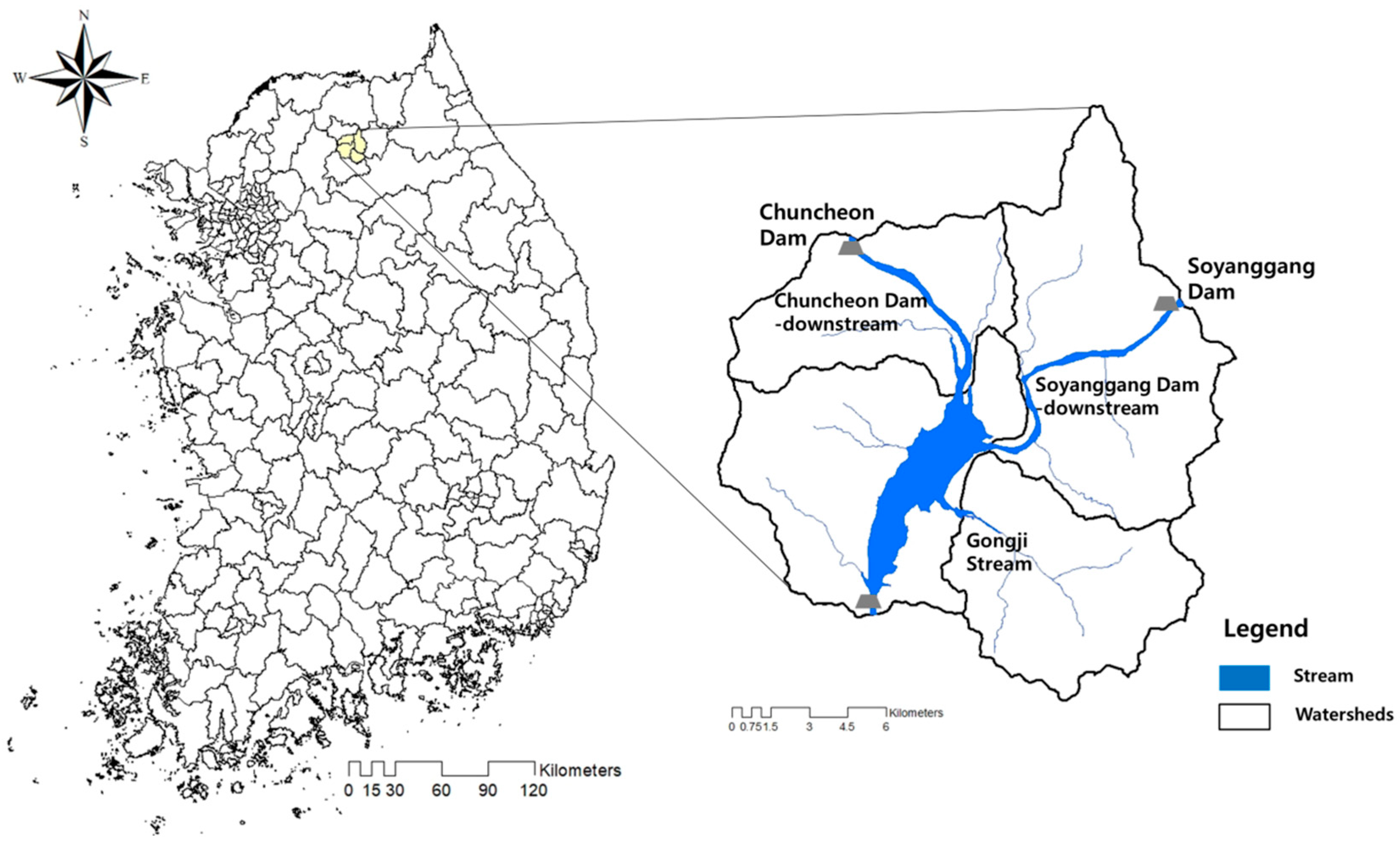
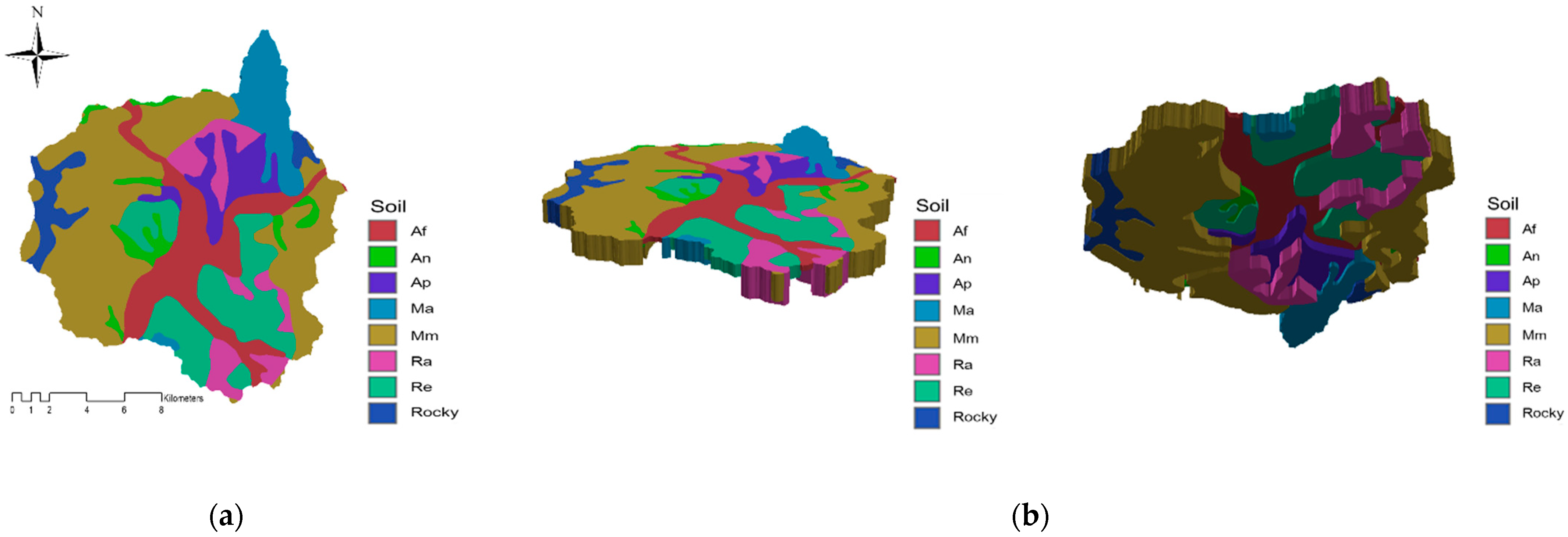
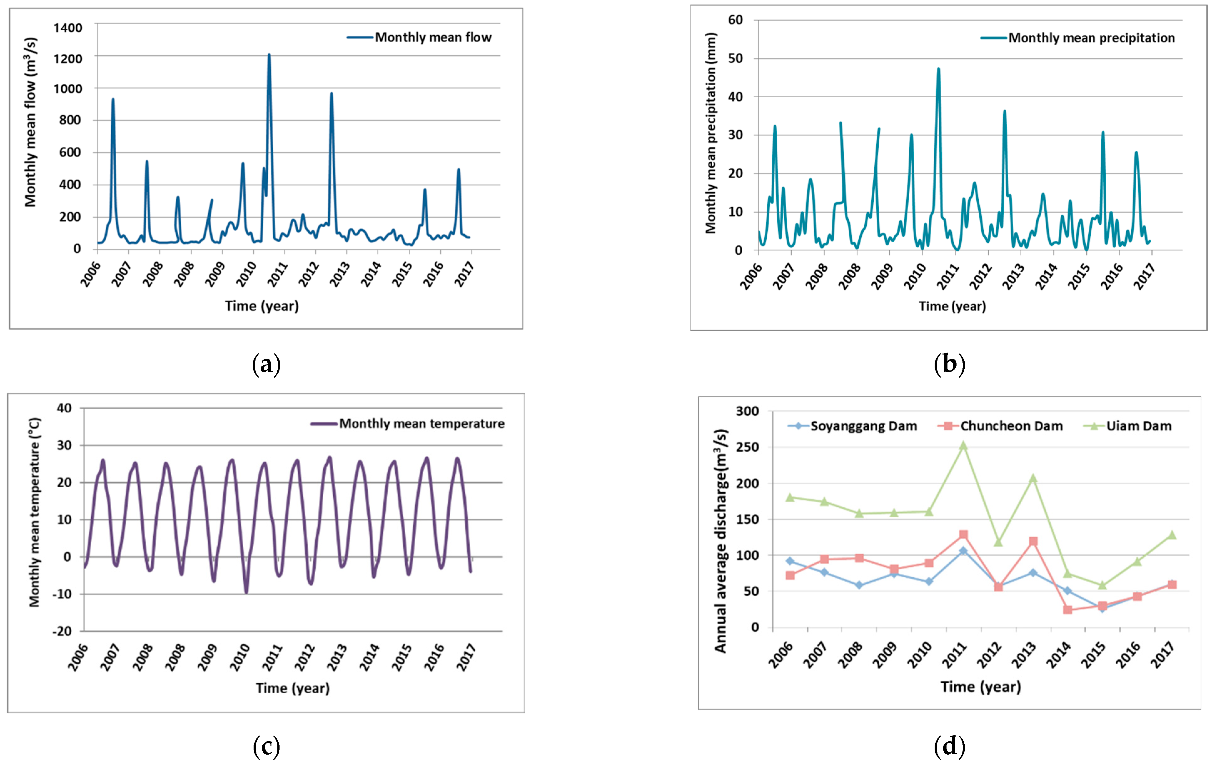
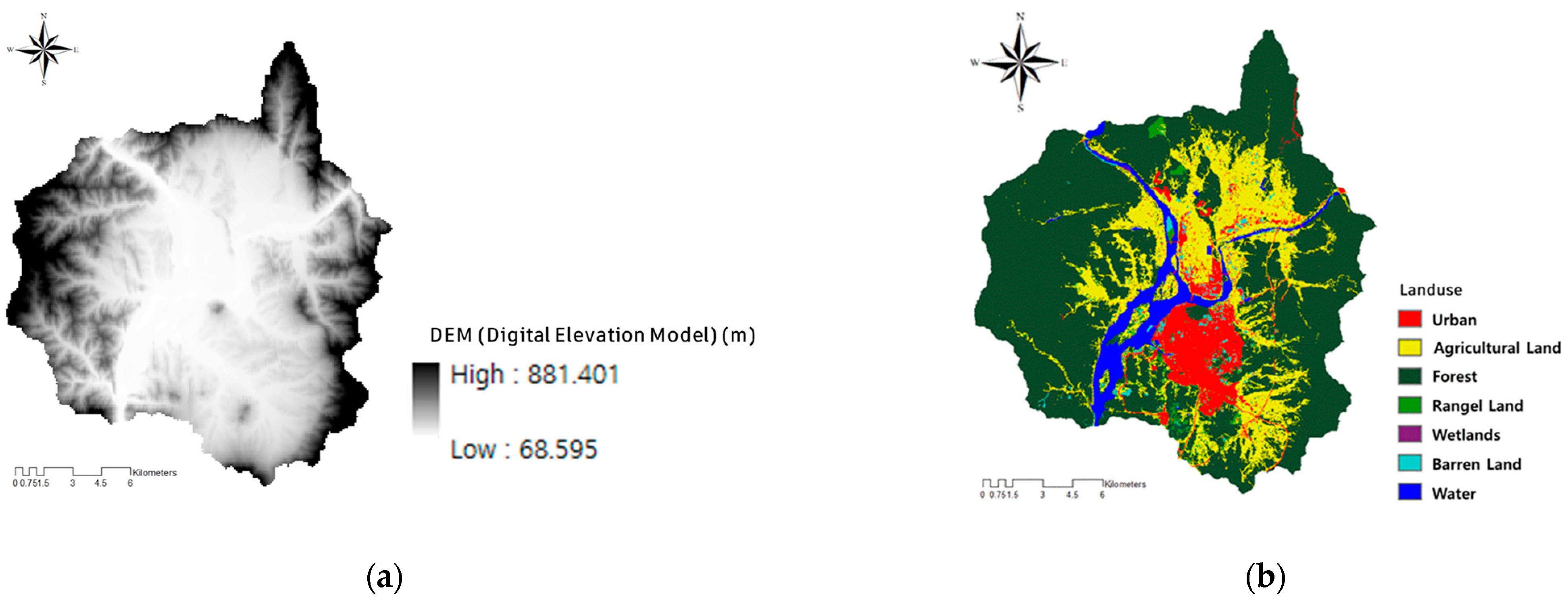
2.1. Study Area
2.2. Description of HSPF Model
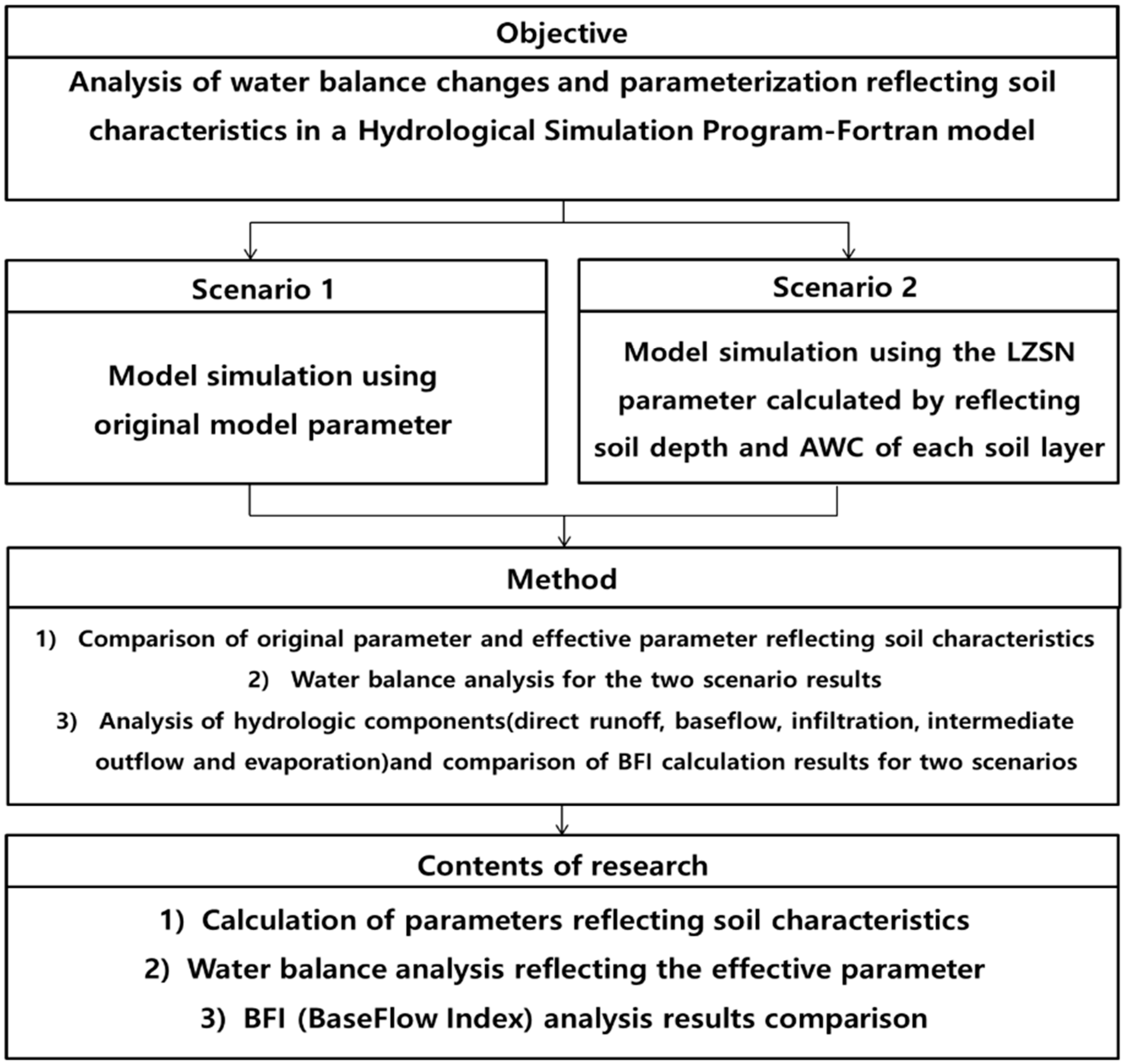
2.3. Estimation of the Effective Parameters Based on Soil Properties and Scenario Analysis
2.4. Baseflow Analysis Using Baseflow Separation Programs (WHAT, BFLOW)
Separation Methods (WHAT, BFLOW)
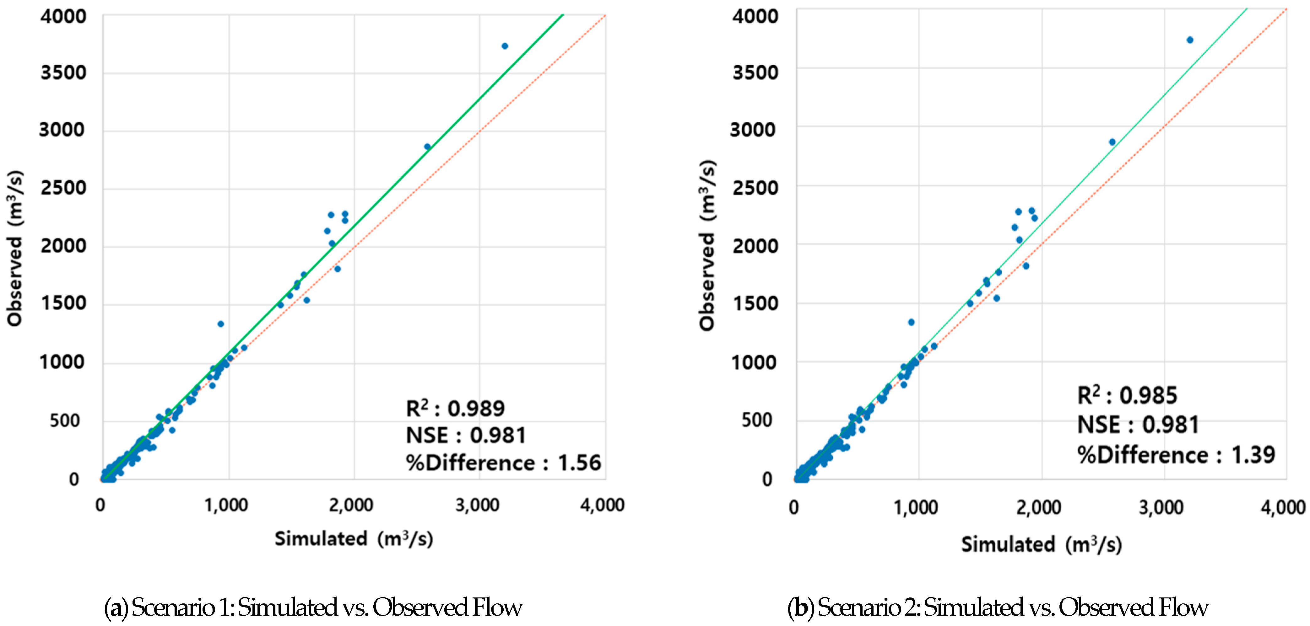
2.5. Evaluation Method
3. Results and Discussion
3.1. Parameter (LZSN) Calculation Considering Soil Characteristics
3.2. Water Balance Analysis for Scenarios 1 and 2
3.3. Baseflow Separation Result for Scenarios 1 and 2
4. Conclusions
- (1)
- With the forest, which occupies the largest area in all sub-watersheds, in Scenario 1 an LZSN value of 0.1 m was applied throughout all sub-watersheds. In Scenario 2, the values of LZSN were 0.16–0.26 m (for each sub-watersheds). For all other land uses, in Scenario 1 an LZSN value of 2 m was applied throughout all sub-watersheds; in Scenario 2 the depth and water capacity of the soil were calculated and applied differently to obtain LZSN for each sub-watershed. In this study, only soil depth and AWC were used as watershed characteristics in calculating the LZSN parameter. However, future studies related to LZSN parameter calculation that reflect more soil properties such as soil adsorption and detachment should be conducted.
- (2)
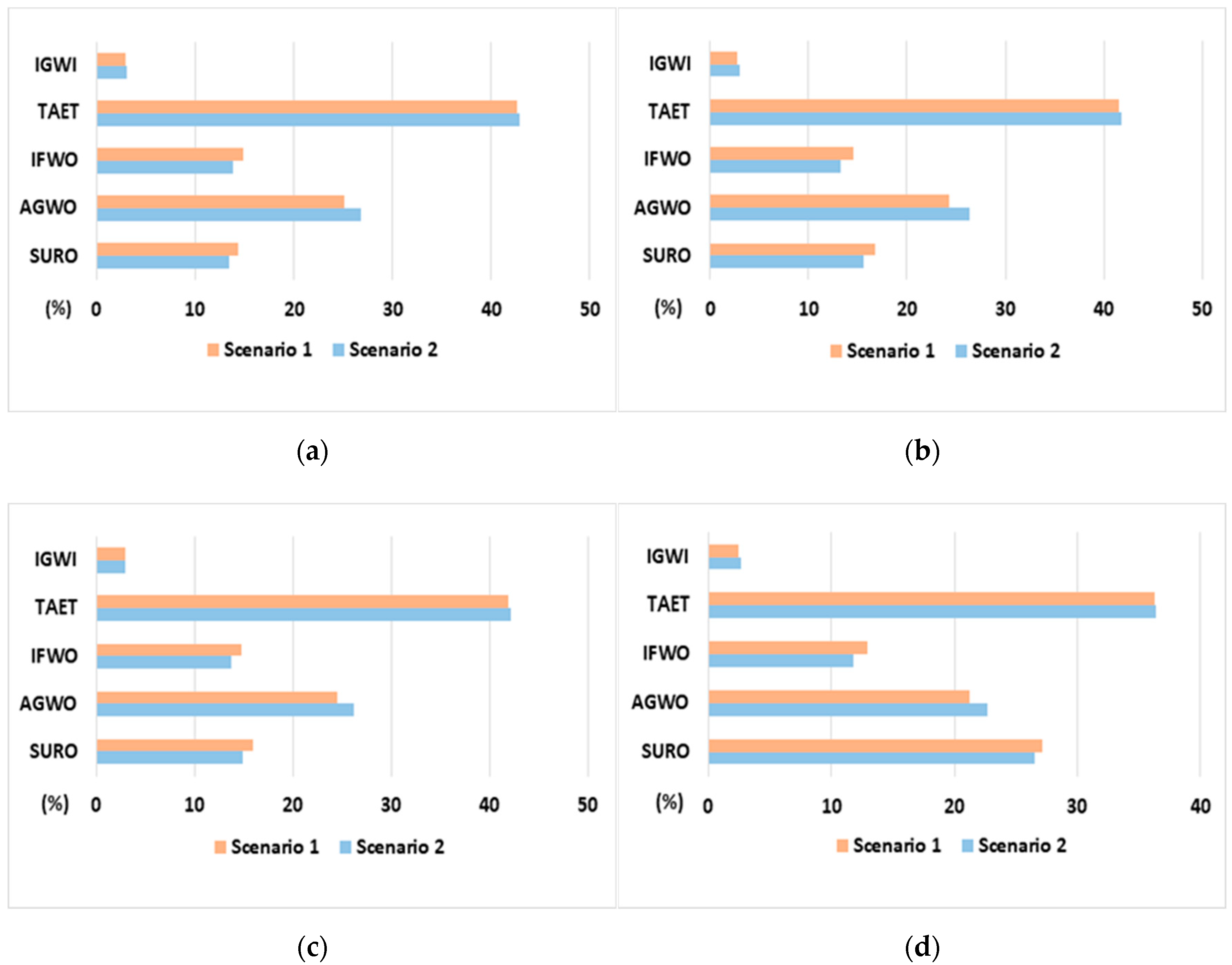
- Water balance analyses by sub-watershed and land use were performed for two scenarios before and after the application of the parameters (LZSN) reflecting soil characteristics. In Scenario 1, the same LZSN value was applied to all land uses except forests, and the water balance analysis showed similar results. In Scenario 2, different LZSN values (reflecting the characteristics of the soil) were applied, and the water balance results differed according to the land use in the sub-watershed. Therefore, even if the total flow was the same, the ratio of each hydrological component varied according to the LZSN value reflecting the soil characteristics.
- (3)
- Due to separating the baseflow using WHAT, the BFI for the measured value was 0.61. BFIs for Scenario 1 and Scenario 2 were 0.65 and 0.61, respectively; the results of Scenario 2 were like the actual measurements. The first pass of BFI by year using BFLOW gave a BFI of 0.65, and the BFIs for Scenarios 1 and 2 were 0.69 and 0.63, respectively. This could be because the BFI was also calculated (using the WHAT system) through analysis of the flow during the dry season because the default value of the model was used, not the value reflecting the runoff characteristics in the BFLOW simulation.
Author Contributions
Funding
Institutional Review Board Statement
Informed Consent Statement
Data Availability Statement
Acknowledgments
Conflicts of Interest
References
- Park, M.S. A Study on Runoff Fluctuation of the Seomjin River Basin by Climate Change. Master’s Thesis, Dongshin University, Jeonlanamdo, Korea, 2012. [Google Scholar]
- Tong, S.T.; Sun, Y.; Ranatunga, T.; He, J.; Yang, Y.J. Predicting plausible impacts of sets of climate and land use change scenarios on water resources. Appl. Geogr. 2012, 32, 477–489. [Google Scholar] [CrossRef]
- Vicente-Serrano, S.M.; Beguería, S.; López-Moreno, J.I. A multiscalar drought index sensitive to global warming: The standardized precipitation evapotranspiration index. J. Clim. 2010, 23, 1696–1718. [Google Scholar] [CrossRef] [Green Version]
- Yang, H.K. Water balance change of watershed by climate change. J. Kor. Geogr. Soc. 2007, 42, 405–420. [Google Scholar]
- Lim, C.S.; Chae, H.S. A Study on Variation in Annual Water Balance I. J. Kor. Water Res. Associat. 2007, 40, 555–570. [Google Scholar] [CrossRef]
- Ahn, S.R.; Park, G.; Jang, C.H.; Kim, S.J. Assessment of climate change impact on evapotranspiration and soil moisture in a mixed forest catchment using spatially calibrated SWAT model. J. Kor. Water Res. Associat. 2013, 46, 569–583. [Google Scholar] [CrossRef] [Green Version]
- Zhang, L.; Dawes, W.R.; Walker, G.R. Response of mean annual evapotranspiration to vegetation changes at catchment scale. Water Resour. Res. 2001, 37, 701–708. [Google Scholar] [CrossRef]
- Yang, D.; Yang, Y.; Xia, J. Hydrological cycle and water resources in a changing world: A review. Geogr. Sustain. 2021, 2, 115–122. [Google Scholar] [CrossRef]
- Crawford, N.H.; Linsley, R.K. Digital Simulation in Hydrology: Stanford Watershed Model IV; Department of Civil Engineering Stanford University: Stanford, CA, USA, 1966. [Google Scholar]
- Abbott, M.B.; Bathurst, J.C.; Cunge, J.A.; O’Connell, P.E.; Rasmussen, J. An introduction to the European Hydrological System—System Hydrologique Europeen, “SHE”, 1: History and philosophy of a physically-based, distributed modelling system. J. Hydrol. 1986, 87, 45–59. [Google Scholar] [CrossRef]
- Beven, K.J.; Kirkby, M.J.; Schofield, N.; Tagg, A.F. Testing a physically-based flood forecasting model (TOPMODEL) for three UK catchments. J. Hydrol. 1984, 69, 119–143. [Google Scholar] [CrossRef]
- Leavesley, G.H. Precipitation-Runoff Modeling System: User’s Manual; U.S. Department of the Interior: Washington, DC, USA, 1984; Volume 83.
- Tsai, L.Y.; Chen, C.F.; Fan, C.H.; Lin, J.Y. Using the HSPF and SWMM models in a high pervious watershed and estimating their parameter sensitivity. Water 2017, 9, 780. [Google Scholar] [CrossRef] [Green Version]
- Arnold, J.G.; Allen, P.M. Automated methods for estimating baseflow and ground water recharge from streamflow records 1. J. Am. Water Res. Associat. 1999, 35, 411–424. [Google Scholar] [CrossRef]
- Lee, S.J. Analysis of Hydrologic Parameters Characteristics in Geumriver Basin Using a HSPF Model. Master’s Thesis, Hanbat National University, Daejeon, Korea, 2017. [Google Scholar]
- Lee, Y.W.; Song, K.D.; Lee, J.C.; Yoon, K.S.; Rhew, D.H.; Lee, S.W.; Lee, S.H. Development of a method for estimating non-point pollutant delivery load of each reference flow with combination of BASINS/HSPF. J. Kor. Soc. Environ. Eng. 2010, 32, 175–184. [Google Scholar]
- Lee, S.; Kim, J.M.; Shin, H.S.; Kwon, S. Evaluation of Riparian Buffer for the Reduction Efficiency of Non-point Sources Using HSPF Model. J. Kor. Soc. Hazard Mitigat. 2019, 19, 341–349. [Google Scholar] [CrossRef] [Green Version]
- Lee, K.S.; Chung, E.S.; Lee, J.S.; Hong, W.P. Analysis of Hydrologic Cycle and BOD Loads Using HSPF in the Anyancheon Watershed. J. Kor. Water Res. Associat. 2007, 40, 585–600. [Google Scholar] [CrossRef]
- Yi, H.S.; Kim, J.K.; Lee, S.U. Development of turbid water prediction model for the Imha dam watershed using HSPF. J. Kor. Soc. Environ. Eng. 2008, 30, 760–767. [Google Scholar]
- Yan, C.; Zhang, W. Effects of model segmentation approach on the performance and parameters of the Hydrological Simulation Program–Fortran (HSPF) models. Hydrol. Res. 2014, 45, 893–907. [Google Scholar] [CrossRef]
- Lee, H.A. Catchment-Scale Hydrological Response to Land Use Change—A Case Study for the Wangsuk River Basin. Master’s Thesis, Seoul National University, Seoul, Korea, 2012. [Google Scholar]
- Seong, C.H. Streamflow modeling in data-scarce estuary reservoir watershed using HSPF. J. Kor. Soc. Agricult. Eng. 2014, 56, 129–137. [Google Scholar] [CrossRef]
- Shin, C.M. Improving HSPF Model’s Hydraulic Accuracy with FTABLES Based on Surveyed Cross Sections. J. Kor. Soc. Water Environ. 2016, 32, 582–588. [Google Scholar] [CrossRef] [Green Version]
- Hedrick, A.R.; Marks, D.; Marshall, H.P.; McNamara, J.; Havens, S.; Trujillo, E.; Sandusky, M.; Robertson, M.; Johnson, M.; Bormann, K.J.; et al. From drought to flood: A water balance analysis of the Tuolumne River basin during extreme conditions (2015–2017). Hydrol. Process. 2020, 34, 2560–2574. [Google Scholar] [CrossRef]
- Chung, E.S.; Lee, K.S. Prioritization of water management for sustainability using hydrologic simulation model and multicriteria decision making techniques. J. Environ. Manag. 2009, 90, 1502–1511. [Google Scholar] [CrossRef]
- Sung, D.G.; Choi, K.S.; Cho, G.S.; Choi, D.H. Parameter Analysis of Runoff Calculation Module in HSPF Model and Estimation using GSIS. J. Kor. Soc. Civil Eng. 2002, 22, 519–528. [Google Scholar]
- Song, H.W.; Lee, H.W.; Choi, J.H.; Park, S.S. Application of HSPF model for effect analyses of watershed management plans on receiving water qualities. J. Kor. Soc. Environ. Eng. 2009, 31, 358–363. [Google Scholar]
- Jo, Y.G. R&D-Comparison of Modeling Techniques Considering Agricultural Non-Point Pollution; Korean National Committee on Irrigation and Drainage: Ansan, Korea, 2014; Volume 53, pp. 48–53. [Google Scholar]
- National Institute of Environment Research. The Method of Calculation Delivery Ratio Based on Basin Model for Total Maximum Daily Load; Ministry of Environment: Sejong, Korea, 2007.
- National Institute of Environment Research. Improvement of HSPF Model for Accuracy of Water Quality Prediction; Ministry of Environment: Sejong, Korea, 2012.
- Jung, S.H.; Rhee, H.P.; Hwang, H.S.; Yoon, C.G. Study on Development of Paddy-RCH Method to Consider Discharge Characteristics of Paddy Field in Watershed Model HSPF. J. Kor. Soc. Environ. Eng. 2019, 41, 311–320. [Google Scholar] [CrossRef] [Green Version]
- Flügel, W.A. Delineating hydrological response units by geographical information system analyses for regional hydrological modelling using PRMS/MMS in the drainage basin of the River Bröl, Germany. Hydrol. Process. 1995, 9, 423–436. [Google Scholar] [CrossRef]
- Duda, P.B.; Hummel, P.R.; Donigian, A.S., Jr.; Imhoff, J.C. BASINS/HSPF: Model use, calibration, and validation. Trans. ASABE 2012, 55, 1523–1547. [Google Scholar] [CrossRef]
- Kang, H.; Hyun, Y.J.; Jun, S.M. Regional estimation of baseflow index in Korea and analysis of baseflow effects according to urbanization. J. Kor. Res. Associat. 2019, 52, 97–105. [Google Scholar]
- Ahn, S.R.; Jang, C.H.; Lee, J.W.; Kim, S.J. Assessment of climate and land use change impacts on watershed hydrology for an urbanizing watershed. J. Kor. Soc. Civil Eng. 2015, 35, 567–577. [Google Scholar] [CrossRef] [Green Version]
- Park, M.J.; Kwon, H.J.; Kim, S.J. Analysis of impacts of land cover change on runoff using HSPF model. J. Kor. Water Res. Associat. 2005, 38, 495–504. [Google Scholar] [CrossRef] [Green Version]
- Park, S.; Lee, H.W.; Lee, Y.S.; Park, S.S. A Hydrodynamic Modeling Study to Analyze the Water Plume and Mixing Pattern of the Lake Euiam. Kor. J. Ecol. Environ. 2013, 46, 488–498. [Google Scholar] [CrossRef]
- Jang, J.H.; Jung, K.W.; Jeon, J.H.; Yoon, C.G. Pollutant loading estimate from Yongdam watershed using BASINS/HSPF. Kor. J. Ecol. Environ. 2006, 39, 187–197. [Google Scholar]
- Johanson, R.C.; Imhoff, J.C.; Davis, H.H. User Manual for Hydrological Simulation Program-FORTRAN (HSPF); Environmental Research Laboratory, Office of Research and Development, US Environmental Protection Agency: Washington, DC, USA, 1980; Volume 80.
- Choi, H.G.; Han, K.Y.; Hwangbo, H.; Cho, W.H. Application analysis of HSPF model considering watershed scale in Hwang River basin. J. Environ. Impact Assess. 2011, 20, 509–521. [Google Scholar]
- NGII Home Page. Available online: https://www.ngii.go.kr/ (accessed on 16 March 2022).
- EGIS Home Page. Available online: https://egis.me.go.kr/ (accessed on 16 March 2022).
- Water Environment Information System Home Page. Available online: http://water.nier.go.kr/ (accessed on 16 March 2022).
- Water Resources Management Information System Home Page. Available online: http://www.wamis.go.kr/ (accessed on 16 March 2022).
- Kim, S.R.; Kim, S.M. Evaluation of HSPF Model Applicability for Runoff Estimation of 3 Sub-watershed in Namgang Dam Watershed. J. Kor. Soc. Water Environ. 2018, 34, 328–338. [Google Scholar]
- Kim, J.K.; Son, K.H.; Noh, J.W.; Lee, S.U. Estimation of suspended sediment load in Imha-Andong watershed using SWAT model. J. Korean Soc. Environ. Eng. 2008, 30, 1209–1217. [Google Scholar]
- Abdi, B.; Bozorg-Haddad, O.; Loáiciga, H.A. Analysis of the effect of inputs uncertainty on riverine water temperature predictions with a Markov chain Monte Carlo (MCMC) algorithm. Environ. Monit. Assess. 2020, 192, 100. [Google Scholar] [CrossRef]
- Ahmadisharaf, E.; Camacho, R.A.; Zhang, H.X.; Hantush, M.M.; Mohamoud, Y.M. Calibration and validation of watershed models and advances in uncertainty analysis in TMDL studies. J. Hydrol. Eng. 2019, 24, 03119001. [Google Scholar] [CrossRef]
- Lim, K.J.; Engel, B.A.; Tang, Z.; Choi, J.; Kim, K.S.; Muthukrishnan, S.; Tripathy, D. Automated web GIS based hydrograph analysis tool, WHAT. J. Am. Water Res. Associat. 2005, 41, 1407–1416. [Google Scholar] [CrossRef]
- Lim, K.J.; Park, Y.S.; Kim, J.; Shin, Y.C.; Kim, N.W.; Kim, S.J.; Jeon, J.H.; Engel, B.A. Development of genetic algorithm-based optimization module in WHAT system for hydrograph analysis and model application. Comput. Geosci. 2010, 36, 936–944. [Google Scholar] [CrossRef]
- Shin, M.H.; Lee, J.A.; Cheon, S.U.; Lee, Y.J.; Lim, K.J.; Choi, J.D. Analysis of the Characteristics of NPS Runoff and Application of L-THIA model at Upper Daecheong Reservoir. J. Kor. Soc. Agricult. Eng. 2010, 52, 1–11. [Google Scholar] [CrossRef]
- Eckhardt, K. How to Construct Recursive Digital Filters for Baseflow Separation. Hydrol. Process. 2005, 19, 507–515. [Google Scholar] [CrossRef]
- Hong, J.Y.; Lim, K.J.; Shin, Y.C.; Jung, Y.H. Quantifying contribution of direct runoff and baseflow to rivers in Han river system, South Korea. J. Kor. Water Res. Associat. 2015, 48, 309–319. [Google Scholar] [CrossRef]
- Lyne, V.; Hollick, M. Stochastic Time-Variable Rainfall-Runoff Modelling; Institution of Engineers Australia: Perth, Australia, 1979; Volume 79, pp. 89–93. [Google Scholar]
- Eckhardt, K. A comparison of baseflow indices, which were calculated with seven different baseflow separation methods. J. Hydrol. 2008, 352, 168–173. [Google Scholar] [CrossRef]
- Bicknell, B.R.; Imhoff, J.C.; Donigian, A.S.; Johanson, R.C. Hydrological Simulation Program—FORTRAN (HSPF). User’s Manual for Release 11. EPA—600/R-97/080; United States Environmental Protection Agency: Athens, GA, USA, 1997.
- Heo, S.G.; Kim, K.S.; Sa, G.M.; Ahn, J.H.; Lim, K.J. Evaluation of SWAT applicability to simulate soil erosion at highland agricultural lands. J. Kor. Soc. Rural Plan. 2005, 11, 67–74. [Google Scholar]
- Moriasi, D.N.; Gitau, M.W.; Pai, N.; Daggupati, P. Hydrologic and water quality models: Performance measures and evaluation criteria. Trans. ASABE 2015, 58, 1763–1785. [Google Scholar] [CrossRef] [Green Version]
- Oh, J.H.; Kim, Y.S.; Ryu, K.S.; Jo, Y.S. Comparison and discussion of MODSIM and K-WEAP model considering water supply priority. J. Korea Water Resour. Assoc. 2019, 52, 463–473. [Google Scholar]
- Kim, H.Y.; Nam, W.H.; Mun, Y.S.; Bang, N.K.; Kim, H.J. Estimation of irrigation return flow on agricultural watershed in Madun reservoir. J. Korean Soc. Agric. Eng. 2021, 63, 85–96. [Google Scholar]
- Lee, D.G.; Song, J.H.; Ryu, J.H.; Lee, J.; Choi, S.K.; Kang, M.S. Integrating the mechanisms of agricultural reservoir and paddy cultivation to the HSPF-MASA-CREAMS-PADDY System. J. Korean Soc. Agric. Eng. 2018, 60, 1–12. [Google Scholar]
- Kim, S.; Song, J.H.; Hwang, S.; Kim, H.G.; Kang, M.S. Development of agricultural water circulation rate considering agricultural reservoir and irrigation district. J. Korean Soc. Agric. Eng. 2020, 62, 83–95. [Google Scholar]
- Srivastava, A.; Kumari, N.; Maza, M. Hydrological response to agricultural land use heterogeneity using variable infiltration capacity model. Water Resour. Manag. 2020, 34, 3779–3794. [Google Scholar] [CrossRef]


| Model Data | Content | Years | Sources |
|---|---|---|---|
| Terrain data | Digital elevation model | 2014 | National Geographic Information Institute |
| Land use | Land use spatial distribution | 2017 | Environmental Geospatial Information Service |
| Meteorological data | Precipitation Evaporation Temperature Wind speed Solar radiation Evapotranspiration Dew point temperature Cloud cover | 2006–2017 | Meteorological Agency |
| Hydrological data | Runoff (KRF 3.0) | 2015 | Environmental Geospatial Information Service |
| Evaluation | Very Good | Good | Satisfactory | Unsatisfactory |
|---|---|---|---|---|
| % Difference | <10 | 10–15 | 15–25 | 25< |
| R2 | >0.8 | 0.7–0.8 | 0.6–0.7 | 0.6> |
| NSE | >0.8 | 0.7–0.8 | 0.5–0.7 | 0.5> |
| Land Use | Estimated Parameter | Default Parameter | |||
|---|---|---|---|---|---|
| Chuncheon Dam—Downstream | Soyanggang Dam—Downstream | Gonggi Stream | Uiam Dam | ||
| Urban | 0.35 | 7.81 | 12.06 | 10.5 | 2 |
| Agricultural Land | 12.34 | 12.33 | 10.08 | 6.61 | |
| Range Land | 6.43 | 6.52 | 7.79 | 9.98 | |
| Wetlands | 15.93 | 5.66 | 26.28 | 7.66 | |
| Barren Land | 8.19 | 6.08 | 11.38 | 6.61 | |
| Water | 2.9 | 4.9 | 4.9 | 4.9 | |
| Forest Land | 7.54 | 10.4 | 6.44 | 8.26 | 3.9 |
| Sub-Basins | Chuncheon Dam—Downstream | Soyanggang Dam—Downstream | Gongji Stream | Uiam Dam | ||||
|---|---|---|---|---|---|---|---|---|
| mm | % | mm | % | mm | % | mm | % | |
| SURO | 200.1 | 14.4 | 238.7 | 16.8 | 443.3 | 27.2 | 224.8 | 15.9 |
| AGWO | 347.3 | 25.1 | 346.6 | 24.3 | 345.4 | 21.2 | 345.7 | 24.5 |
| IFWO | 206.8 | 14.9 | 207.8 | 14.6 | 210.5 | 12.9 | 208.4 | 14.8 |
| TAET | 591.4 | 42.7 | 591.2 | 41.5 | 590.8 | 36.3 | 591.0 | 41.9 |
| IGWI | 39.8 | 2.9 | 39.7 | 2.8 | 39.6 | 2.4 | 39.6 | 2.9 |
| SUM | 1385.5 | 100.0 | 1424.1 | 100.0 | 1629.6 | 100.0 | 1409.5 | 100.0 |
| Sub-Basins | Chuncheon Dam—Downstream | Soyanggang Dam—Downstream | Gongji Stream | Uiam Dam | ||||
|---|---|---|---|---|---|---|---|---|
| mm | % | mm | % | mm | % | mm | % | |
| SURO | 185.7 | 13.4 | 222.0 | 15.6 | 432.9 | 26.5 | 210.6 | 14.9 |
| AGWO | 370.9 | 26.8 | 374.5 | 26.3 | 370.3 | 22.7 | 369.6 | 26.2 |
| IFWO | 190.8 | 13.8 | 189.8 | 13.3 | 192.0 | 11.8 | 192.7 | 13.7 |
| TAET | 594.5 | 42.9 | 594.6 | 41.8 | 594.4 | 36.4 | 594.6 | 42.2 |
| IGWI | 42.6 | 3.1 | 42.8 | 3.0 | 42.4 | 2.6 | 42.3 | 3.0 |
| SUM | 1384.4 | 100.0 | 1423.8 | 100.0 | 1631.9 | 100.0 | 1409.9 | 100.0 |
| Land Use | SURO | TAET | IGWI | SUM | ||||
|---|---|---|---|---|---|---|---|---|
| mm | % | mm | % | mm | % | mm | % | |
| Urban | 284.8 | 13.3 | 927.6 | 43.3 | 928.4 | 43.4 | 2140.7 | 100.0 |
| Agricultural Land | 24.4 | 13.3 | 79.3 | 43.3 | 79.4 | 43.4 | 183.0 | 100.0 |
| Forest | 1026.6 | 12.2 | 3675.3 | 43.7 | 3701.4 | 44.1 | 8403.3 | 100.0 |
| Range Land | 40.3 | 13.3 | 131.4 | 43.3 | 131.5 | 43.4 | 303.2 | 100.0 |
| Wetlands | 319.5 | 13.3 | 1040.9 | 43.3 | 1041.8 | 43.4 | 2402.1 | 100.0 |
| Barren Land | 16.9 | 13.3 | 55.1 | 43.3 | 55.2 | 43.4 | 127.2 | 100.0 |
| Water | 658.0 | 100.0 | 0.0 | 0.0 | 0.0 | 0.0 | 658.0 | 100.0 |
| Land Use | SURO | TAET | IGWI | SUM | ||||
|---|---|---|---|---|---|---|---|---|
| mm | % | mm | % | mm | % | mm | % | |
| Urban | 236.3 | 11.6 | 890.2 | 43.9 | 903.4 | 44.5 | 2029.9 | 100.0 |
| Agricultural Land | 19.6 | 11.3 | 76.1 | 43.9 | 77.7 | 44.8 | 173.4 | 100.0 |
| Forest | 911.8 | 11.5 | 3495.0 | 43.9 | 3558.9 | 44.7 | 7965.7 | 100.0 |
| Range Land | 33.1 | 11.5 | 126.1 | 43.9 | 128.3 | 44.6 | 287.5 | 100.0 |
| Wetlands | 266.7 | 11.7 | 998.7 | 43.8 | 1012.5 | 44.5 | 2277.9 | 100.0 |
| Barren Land | 14.4 | 11.9 | 52.8 | 43.8 | 53.6 | 44.3 | 120.6 | 100.0 |
| Water | 624.0 | 100.0 | 0.0 | 0.0 | 0.0 | 0.0 | 624.0 | 100.0 |
| Average Streamflow | Average Direct Runoff | Average Baseflow | |
|---|---|---|---|
| Uiam Dam | 3.18 (100) | 1.23 (38.7) | 1.95 (61.3) |
| Scenario 1 | 3.12 (100) | 1.09 (35.0) | 2.03 (65.0) |
| Scenario 2 | 3.13 (100) | 1.21 (38.7) | 1.92 (61.3) |
| Annual Average Baseflow Index (BFI) | |
|---|---|
| Observed | 0.65 |
| Scenario 1 | 0.69 |
| Scenario 2 | 0.63 |
Publisher’s Note: MDPI stays neutral with regard to jurisdictional claims in published maps and institutional affiliations. |
© 2022 by the authors. Licensee MDPI, Basel, Switzerland. This article is an open access article distributed under the terms and conditions of the Creative Commons Attribution (CC BY) license (https://creativecommons.org/licenses/by/4.0/).
Share and Cite
Kim, S.; Kim, J.; Kang, H.; Jang, W.S.; Lim, K.J. Analysis of Water Balance Changes and Parameterization Reflecting Soil Characteristics in a Hydrological Simulation Program—FORTRAN Model. Water 2022, 14, 990. https://doi.org/10.3390/w14060990
Kim S, Kim J, Kang H, Jang WS, Lim KJ. Analysis of Water Balance Changes and Parameterization Reflecting Soil Characteristics in a Hydrological Simulation Program—FORTRAN Model. Water. 2022; 14(6):990. https://doi.org/10.3390/w14060990
Chicago/Turabian StyleKim, Soohong, Jonggun Kim, Hyeongsik Kang, Won Seok Jang, and Kyoung Jae Lim. 2022. "Analysis of Water Balance Changes and Parameterization Reflecting Soil Characteristics in a Hydrological Simulation Program—FORTRAN Model" Water 14, no. 6: 990. https://doi.org/10.3390/w14060990