
Why the Effect of CO2 on Potential Evapotranspiration Estimation Should Be Considered in Future Climate
by
Jian Zhou
1,†, 
Shan Jiang
1,†,
Buda Su
1,*,
Jinlong Huang
1,
Yanjun Wang
1,
Mingjin Zhan
2,
Cheng Jing
1 and
Tong Jiang
1,* 1
Collaboration Innovation Center on Forecast and Evaluation of Meteorological Disasters, Institute for Disaster Risk Management, School of Geographical Sciences, Nanjing University of Information Science & Technology, Nanjing 210044, China
2
Jiangxi Eco-Meteorological Center, Nanchang 330000, China
*
Authors to whom correspondence should be addressed.
†
These authors contributed equally to this work.
Water 2022, 14(6), 986; https://doi.org/10.3390/w14060986
Submission received: 9 February 2022
/
Revised: 14 March 2022
/
Accepted: 18 March 2022
/
Published: 21 March 2022
(This article belongs to the Section Hydrology)
Abstract
:Potential evapotranspiration (PET) is an important factor that needs to be considered in regional water management and allocation; thus, the reasonable estimation of PET is an important topic in hydrometeorology and other related fields. There is evidence that increased CO2 concentration alters the physiological properties of vegetation and thus affects PET. In this study, changes in PET with and without the CO2 effect over China is investigated using seven CMIP6-GCMs outputs under seven shared socioeconomic pathways (SSPs) based scenarios (SSP1-1.9, SSP1-2.6, SSP2-4.5, SSP3-7.0, SSP4-3.4, SSP4-6.0, and SSP5-8.5), as well as the contribution rate of CO2 on PET in different climatic regions. Changes in estimated PET based on modified Penman–Monteith (PM) method that considers the CO2 effect is compared with the traditional PM method to examine how PET quantity varies (differences) between these two approaches. The results show that the PET values estimated by the two methods explored opposite trends in 1961–2014 over entire China; it decreases with consideration of CO2 but increases without consideration of CO2. In the future, overall PET is projected to increase under all scenarios during 2015–2100 for China and its three sub-regions. PET generally tends to grow slower when CO2 is taken into account (modified PM approach), than when it is not (traditional PM method). In terms of differences in the estimated PET by the two methods, the difference between the two adopted methods increased in China and its sub-regions for the 1961–2014 period. In the future, the difference in estimated PET is anticipated to continuously increase under SSP3-7.0 and SSP5-8.5. Spatially, a much greater extent of difference is found in the arid region. Across the arid region, the PET difference is projected to be the highest at 138% in the mid-term (2041–2060) with respect to the 1995–2014 period, whereas it tends to increase slower in the long-term period (2081–2100). Importantly, CO2 is found to be the most dominant factor (−154.2% contribution) to have a great effect on PET changes across the arid region. Our findings suggest that ignorance of CO2 concentration in PET estimation will result in significant overestimation of PET in the arid region. However, consideration of CO2 in PET estimation will be beneficial for formulating strategies on future water resource management and sustainable development at the local scale.
1. Introduction
Evapotranspiration is related not only to the water balance and phase change of water [1,2,3], but also to the climate system, linking the water, energy, and carbon cycles on the land surface [4,5], and is directly affected by climate change. It can absorb a fraction of the available annual solar radiation globally received at the Earth’s surface and return approximately 60% of the available annual land precipitation to the atmosphere [6,7,8]. Potential evapotranspiration (PET) reflects the evaporative power of the atmosphere, which refers to the maximum possible water loss that can be achieved on the land surface under certain meteorological conditions when the water supply is not restricted [9,10,11]. PET is vital for hydrologic cycle, water resource assessments, crop water requirement, and irrigation demand assessments, especially in the context of global warming. It has been reported that the global surface temperature was 1.09 °C higher in 2011–2020 than in 1850–1900, and climate change will accelerate the water cycle due to increased land evapotranspiration [12]. Such changes in PET largely influence further escalation of different climatic extremes (i.e., Drought) in terms of frequency duration and intensity [13,14]. Therefore, the research on prospective changes in future PET under changing climate has become a great concern for global communities to ensure better water resource management.
Unlike other meteorological elements, PET cannot be measured directly by using any instruments, but rather is estimated (often theoretically) based on other meteorological variables. Numerous methods have been proposed in past decades to estimate PET. These methods can be classified into three types according to the required inputs, i.e., temperature-based methods, radiation-based methods, and synthesis methods [15,16,17]. As a typical equation that combines the aerodynamic term and the energy term, the Penman–Monteith (PM) formula [18] recommended by the Food and Agriculture Organization (FAO) is the most widely used PET estimation model in the field of hydrometeorology. It is worth mentioning that the eco-hydrological water cycle such as evapotranspiration is one of the main drivers of plant productivity [19], and the characteristics of plant physiological and metabolic processes will also feed back into the eco-hydrological cycle. However, the PM formula by FAO assumes that the surface resistance (rs) is a constant (70 s/m), which is suitable for the current climate conditions but not for a warming world [20,21,22]. It is known that high CO2 concentrations cause partial stomatal closure of vegetation, which reduces stomatal conductance of vegetation [23,24,25]. Due to the continuously increasing CO2 concentration in the future, rs will also increase accordingly. That is to say, the increase in CO2 concentration should have an effect on PET, and omitting this effect could lead to the overestimation of droughts. A modified PM formula that considers CO2 concentration is proposed as an alternative for estimating PET under a climate change background [21,26]. Thus, it is of great importance to have detailed information on how CO2 inclusion will influence the changes in future PET over different climatic regions.
Previous PET-related studies have mainly focused on the detection and projection of its spatiotemporal changes [17,27,28,29,30,31,32,33,34] and its influencing factors [15,35,36,37]. However, the effect of increased CO2 concentrations on PET has been ignored in most studies, and an understanding of the CO2 effect in different climatic zones is still lacking. In this paper, how large a difference exists between PET with and without the CO2 effect will be revealed for three defined future periods namely near-term (2021–2040), mid-term (2041–2060), and long-term (2081–2100) with special emphasis given on different climatic zones in China. Moreover, the effect of each influential factor (i.e., temperature, rs, CO2, etc.) on PET is also epitomized. Notably, seven global climate models (GCMs) output under seven Shared Socioeconomic Pathways (SSPs)-based climate change scenarios (SSP1-1.9, SSP1-2.6, SSP2-4.5, SSP3-7.0, SSP4-3.4, SSP4-6.0, and SSP5-8.5) from the 6th phase of Coupled Model Intercomparison Project (CMIP6) are used. However, it is expected that the adoption of the advanced multi-models, a large number of future scenarios, and consideration of the modified PET approach with the updated CO2 data will provide more reasonable and reliable results in this paper.
2. Materials and Methods
2.1. Study Area
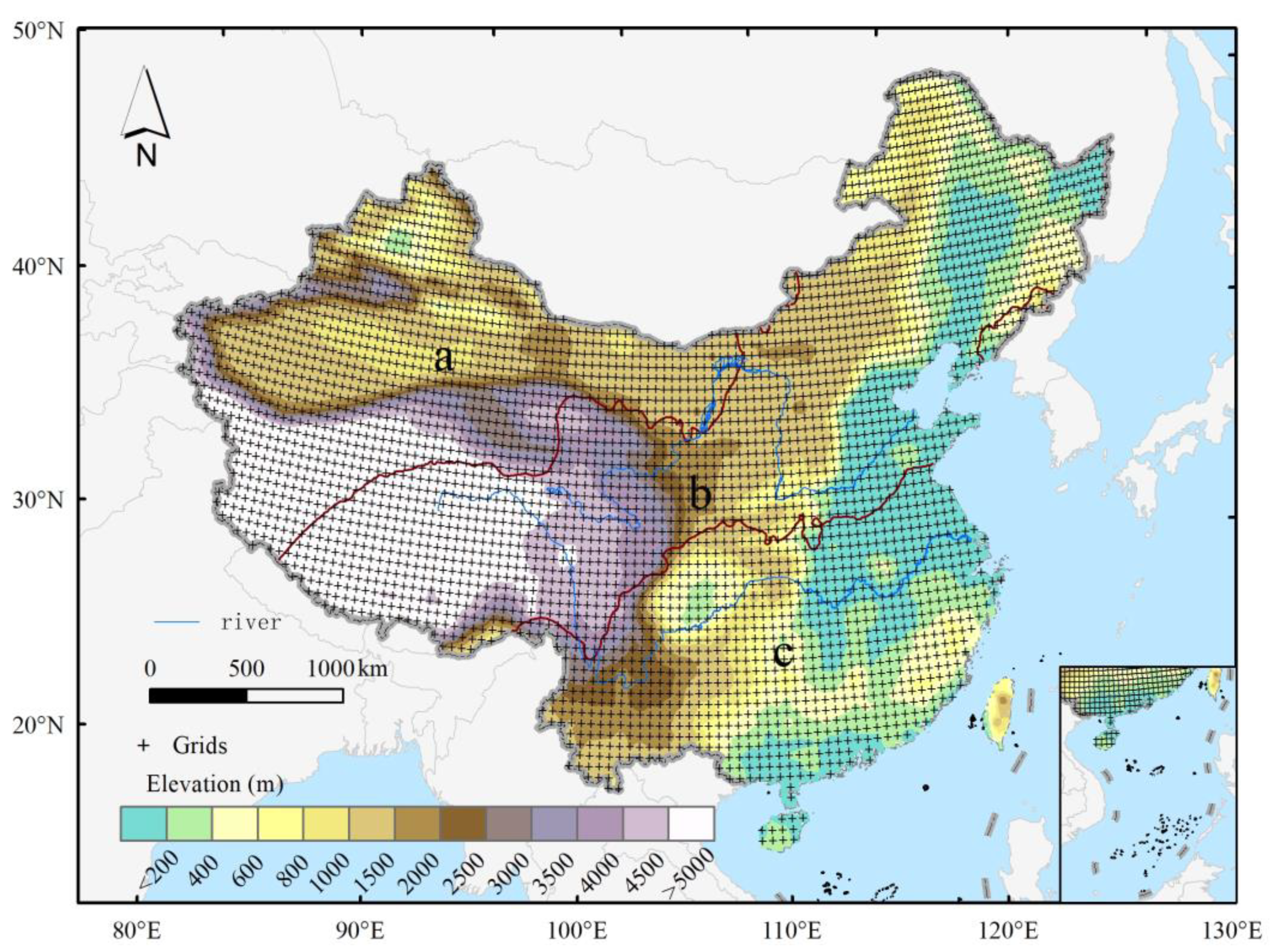
China is one of the world’s largest countries with complex terrain, which is surrounded by the Pacific Ocean to the east and the Qinghai-Tibet Plateau to the southwest (Figure 1). Altogether, the large north-south and east-west spans, varying elevation, diverse surface conditions, and mountain trends interactively created the complexity of its climate conditions and environmental characteristics. Climatologically, the responses of different climatic zones to global climate change are generally different. Annual average PET values are found to vary for three main climatic regions (i.e., the arid region, the semi-arid and semi-humid region, and the humid region). For precipitation, annual precipitation < 200 mm is found in the arid region, while it varies from 200–800 mm across the semi-arid and semi-humid region, and the humid region experiences annual precipitation of greater than 800 mm. In general, precipitation is mainly concentrated in summer because warm and wet air from the ocean brings sufficient water vapour to most of China under the significant influence of the East Asian monsoon. Highly concentrated precipitation leads to frequent flood and drought disasters, whereas, the changes in PET lead to further intensification of such events in China [38].
2.2. Datasets
In this study, the input monthly climate parameters including mean temperature, maximum temperature, minimum temperature, precipitation, relative humidity, air pressure, radiation, and wind speed under seven SSP-based scenarios (SSP1-1.9, SSP1-2.6, SSP2-4.5, SSP3-7.0, SSP4-3.4, SSP4-6.0, and SSP5-8.5) are obtained from the CMIP6 achieve. Seven (07) GCMs outputs are selected in this paper based on the availability of the essential variables (above mentioned) under these quest scenarios. The datasets are downloaded for the two periods: the historical period (1961–2014) and the projection period (2015–2100). The outputs for the projection period of each model are considered under seven selected SSPs (SSP1-1.9, SSP1-2.6, SSP2-4.5, SSP3-7.0, SSP4-3.4, SSP4-6.0, and SSP5-8.5), which combine Shared Socioeconomic Pathways and Representative Concentration Pathways. Notably, as the multi-model ensemble mean can effectively reduce the uncertainty of climate simulation, the ensemble mean of the seven GCMs is adopted in this paper. The details of the seven GCMs are presented in Table 1.
For the observation dataset, a set of observed meteorological data from the China Meteorological Administration is used as the basis of bias correction as well as downscaling of GCMs outputs to a common resolution of 0.5°. The detailed process of downscaling and bias correction methods is described in the studies by Su et al., 2016 and Su et al., 2018 [39,40]. We collected daily observation data from 2479 ground-based stations in China for 1961–2019, including precipitation, mean temperature, maximum temperature, minimum temperature, relative humidity, air pressure, wind speed, sunshine duration, etc. After data quality control and outlier tests (such as high and low anomalies, temporal anomalies, and spatial anomalies), the sites with more than 5% missing data were eliminated, and a total of 2072 meteorological stations with relatively complete data series were selected in this study.
CO2 concentration data is produced by the University of Melbourne for a time period from 2000 years ago to the year 2500 with a spatial resolution of 0.5° [41,42]. The historical CO2 data are recorded for centuries of ice core/firn data and multi-decadal measurements by the National Oceanic & Atmospheric Administration (NOAA) and the Advanced Global Atmospheric Gases Experiment (AGAGE) networks. The CO2 concentration for the future period is estimated by the Model for the Assessment of Greenhouse Gas Induced Climate Change (MAGICC), which deduces CO2 concentrations under the latest different SSPs. The evolutions of CO2 concentrations are used by the Earth System Models as part of the CMIP6 project (https://greenhousegases.science.unimelb.edu.au/#!/view (accessed on 9 February 2022)). In this paper, CO2 concentration data are used from these sources for the 1961–2100 period to estimate PET.
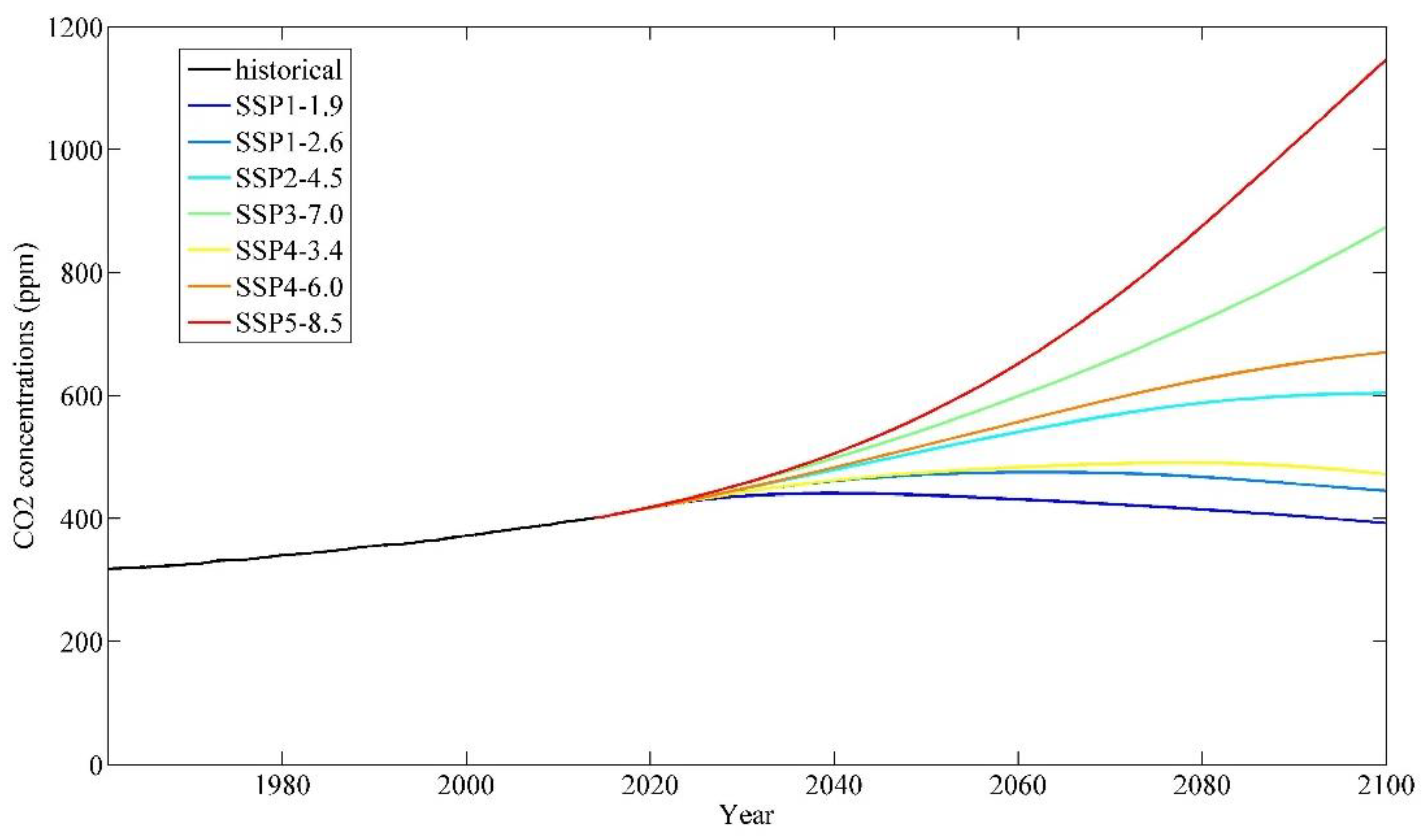
In Figure 2, changes in CO2 concentration from 1961 to 2100 are demonstrated to describe the overall status of CO2 in China. From 1961 to 2014, the CO2 concentration was increased rapidly in China, at a rate of approximately 16 ppm/10a. In 2014, the CO2 concentration reached approximately 401 ppm, over 1.4 times higher than the preindustrial level (278 ppm). Different SSPs have been used to estimate future CO2 concentrations. It is estimated that only under SSP1-1.9, CO2 concentration can be less than the current level at the end of the century. Under SSP1-2.6 and SSP4-3.4, the CO2 concentration is inclined to increase first and then decrease, which could reach approximately 445 ppm and 472 ppm by the end of the century under these two scenarios, respectively. Under SSP2-4.5 and SSP4-6.0, the rates of increase in CO2 concentration gradually slow down but can reach 604 ppm and 671 ppm by 2100 under these two scenarios, respectively. The CO2 concentration is estimated to grow continuously at a high speed under SSP3-7.0 and SSP5-8.5, with growth rates of approximately 55 ppm/10a and 88 ppm/10a, and will reach approximately 875 ppm and 1147 ppm, respectively, by the end of the century (Figure 2).
2.3. Estimation of Potential Evapotranspiration
In this paper, the estimation of PET adopts the following two methods:
One is the commonly used PM algorithm recommended by the FAO, which combines the aerodynamic term with the energy term and is applicable to an idealized reference crop surface with the determined parameter (rs = 70 s m−1, vegetation height of 0.12 m and surface albedo of 0.23) [18].
The other one is the modified PM algorithm (PM_CO2), which takes rising CO2 concentrations into account to show changes in surface resistance with global warming. The derivation of PM_CO2 algorithm is roughly as follows, and the specific method is shown in Yang et al., 2019 and 2020 [20,21]:
By comparing the PM algorithm above with the primitive PM formula for undetermined parameters PM algorithm, the following equation can be obtained.
Surface resistance (rs) adopts parameters of reference crop surface (70 s m−1), and is computed by:
The mean CO2 concentration in 1861–1960, which is about 300 ppm, as the intercept of function between rs and CO2 concentration.
According to Yang et al., 2019 [20], rs_300 represents is surface resistance at 300 ppm of CO2 set as 70 s m−1, and can be calculated as around 0.05 s m−1 ppm−1 based on historical period. Substituting the above three equations into the first method makes it possible to arrive at the modified PM algorithm:
where ra represents aerodynamic resistance. Δ (kPa·°C−1) is the slope of the saturated water pressure curve. Rn (MJ·m−2·d−1) represents the net radiation, and G (MJ·m−2·d−1) is the heat flux into the ground. γ (kPa·°C−1) is the psychrometric constant. es (kPa) and ea (kPa) are the saturation vapour pressure and actual vapour pressure, respectively. T (°C) and U2 (m·s−1) represent the air temperature and wind speed at a height of 2 m, respectively. CO2 (ppm) represents the carbon dioxide concentration.
2.4. Evaluation of Simulation Capability for Climate Models
The spatial correlation coefficient is a common method to analyse the correlation between two grid layers. The correlation coefficient of the ensemble mean of GCMs and the observation is used as one criterion to evaluate the simulation capability of GCMs. The formula is
where is the observed meteorological element, is the same meteorological element from the multi-model ensemble, and N is the number of grid points (3826 in this paper).
2.5. Contribution Rates Calculation
In this paper, a method introduced by Sun et al., (2017) [43] is used to analyse the contribution rates of each influential factor on PET changes in China, which has the advantage of being able to strip out the contributions of the elements that interact with each other. In this study, temperature, relative humidity, wind speed, radiation, and carbon dioxide concentration can be seen as the major driving factors to PET changes, and these five factors sensitivity experiments were performed for the period of 2015–2100 by controlling variables approach. For each sensitivity experiment, one driving factor from only 2015 and other factors from 2015 to 2100 was used. For example, when a sensitivity experiment is performed on temperature, repeatedly employed temperature data from 2015, but used data for the other factors from 2015 to 2100 as the inputs for calculating PET, and the trend for PET obtained includes the contribution of other four elements.
where denotes the trend of PET which keeps the temperature constant; k represents factors; and n is the number of factors, which is 5 here.
The same approach is applied to the sensitivity experiments of the other four elements, and then five sets of equations are obtained. The contribution formula of a single element is obtained by solving the equations as follows:
where i denotes the factor to be solved for contribution; Ti represents the trend of PET which keep the factor (i) constant and Tk represents the trend of PET which keeps the factor constant except for i.
3. Results
3.1. Assessment of GCMs’ Simulation Capability
In this section, the observed temperature and precipitation data for 1961–2014 are selected to evaluate the simulation capability of the GCMs in the regional climate in China.
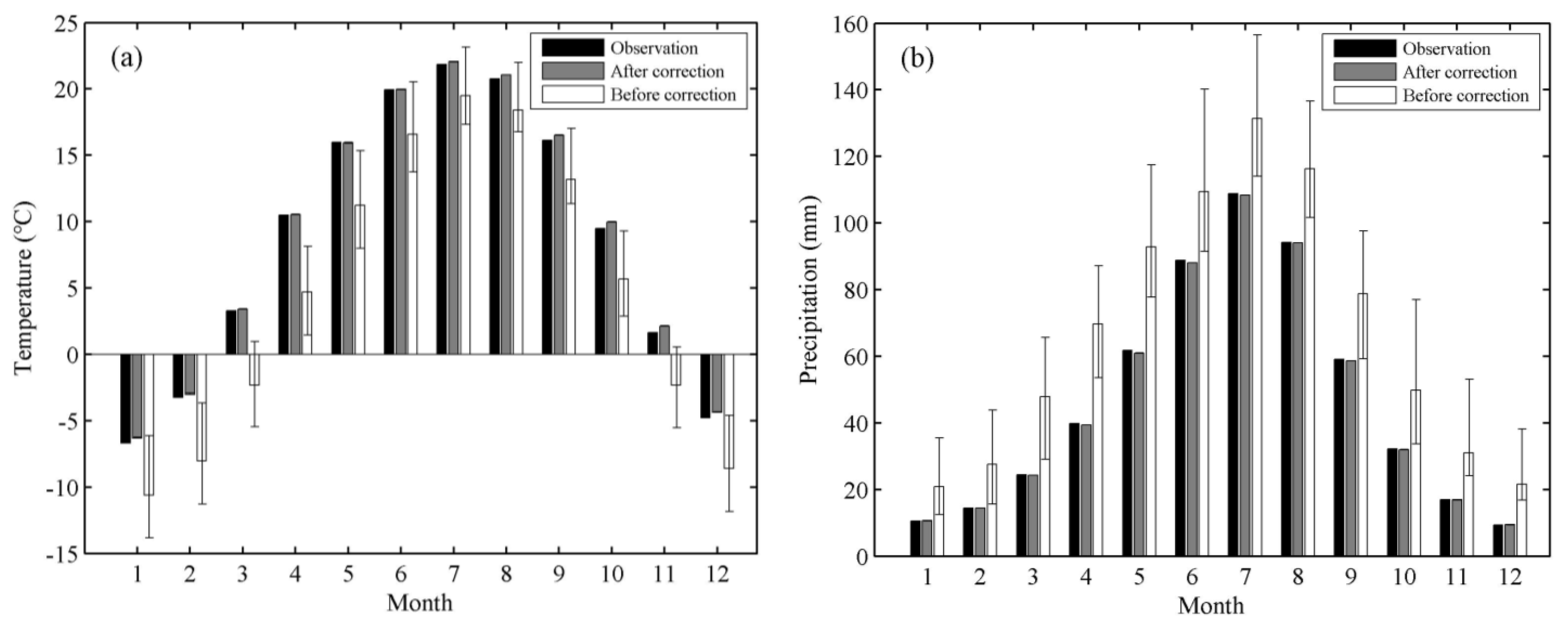
A single model may have relatively great uncertainty, so a multi-model ensemble is adopted to reduce the uncertainty caused by the models. Before bias correction, the simulated monthly temperature is obviously lower than the observed data with a margin of error for approximately 2.3 °C to 5.8 °C. After bias correction, the result of the simulated monthly mean temperature by the multi-model ensemble is slightly higher than the observation except in May, but the bias-corrected GCMs can capture the inner-annual distribution of temperature quite satisfactorily, with monthly mean temperatures in January, February, and December less than 0 °C and that in July being the highest. The differences in the simulated and observed temperatures are smaller in April, May, and June than in the other months, with errors below 0.1 °C, while the maximum difference is approximately 0.5 °C in November (Figure 3a).
Before bias correction, although the inner-annual distribution pattern of precipitation is captured quite well by GCMs, with more precipitation in summer and less precipitation in winter, the amount of precipitation in each month was overestimated systematically, with a maximum error of approximately 31.1 mm in May and a minimum error of approximately 10.3 mm in January. After bias correction, the GCMs somewhat overestimate the monthly precipitation in winter (the error range is no more than 0.1 mm), and slightly underestimate precipitation in the other seasons. In February, March, and November, the precipitation error between the simulated and observed values is only 0.03 mm. The relatively large errors between simulated and measured precipitation are found to be 0.9 mm and 0.7 mm, respectively, in May and June. The annual precipitation is 560 mm and 557 mm by measurement and bias correction, and the error between the two is only 0.6%. That is to say, the simulation of precipitation by climate models is improved visibly after bias correction, and GCMs can satisfactorily capture both the inner-annual distribution pattern and quantity of precipitation in China (Figure 3b).
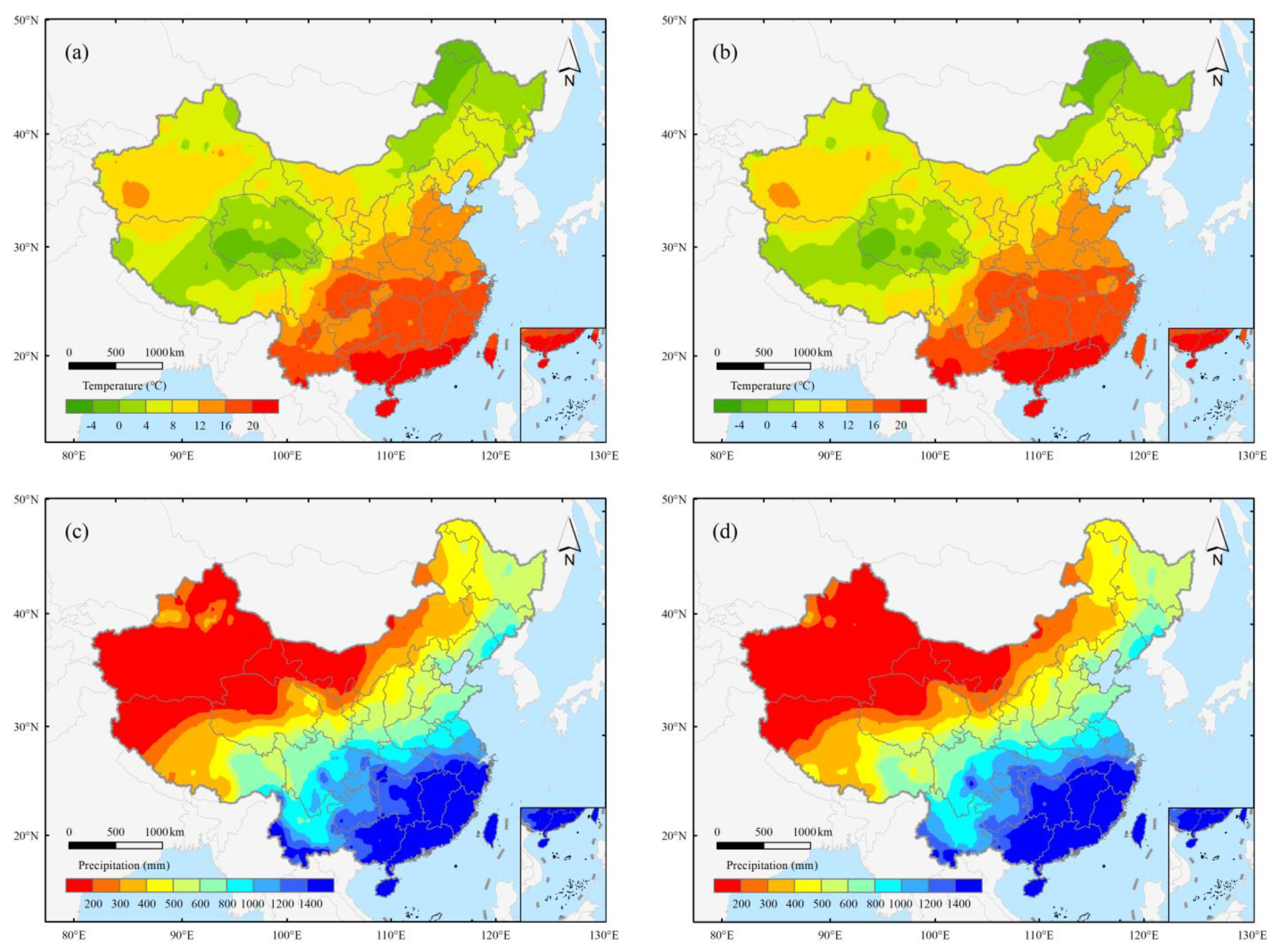
The spatial distribution of annual mean temperature by the multi-model ensemble during 1961–2014 is roughly consistent with the measured results (Figure 4a,b). The annual mean temperatures of the GCMs ensemble mean and observational data both show the characteristics of a decrease from south to north, with temperatures above 16 °C in most of southern China (even exceeding 20 °C in the southmost coastal region), approximately 12–16 °C in eastern China, and approximately 8 °C in most of northwestern and northeastern China. Although the GCMs underestimate the average annual temperature slightly on the Tibetan Plateau, the spatial distributions of the simulated and measured data are basically the same in China, and their spatial correlation coefficient exceeds 0.97 (significant at the 0.01 level).
For the spatial distribution of annual precipitation, both of observation and simulation show a feature of more precipitation in the south and less precipitation in the north, decreasing from the south-eastern coast to the northwest. The 800 mm isoline is roughly along the Qinling Mountains and Huaihe River. The annual precipitation in the south-eastern coastal area can reach more than 1200 mm, whereas north-western China receives less than 200 mm. The spatial correlation coefficient between the multi-model ensemble mean and the observation is more than 0.95 (significant at the 0.01 level), reflecting strong spatial consistency (Figure 4c,d).
3.2. Effect of CO2 on PET
The effect of CO2 on PET is quantified by comparing the results from the two algorithms (Table 2). Taking China as a whole, PET shows a decreasing trend at a rate of 0.4 mm/10a when the effect of CO2 is considered but increases by 1.1 mm/10a without the CO2 effect for 1961–2014. In the arid region as well as the semi-arid and semi-humid region, the PET estimated by the two algorithms showed a positive trend but increased faster in the case without considering the CO2 effect, with rates of 3.6 mm/10a versus 1.2 mm/10a in the arid region and 2.8 mm/10a versus 0.7 mm/10a in the semi-arid and semi-humid region, respectively. For the humid region, both PET values exhibit a downtrend at rates of 4.0 mm/10a and 2.7 mm/10a, respectively. The global dimming could be one reason why PET decreases in the humid region. Studies have pointed out that the PET trend in southern China is highly correlated with the change in global surface solar radiation, which has transitioned from decreasing to increasing, with the late 20th century acting as the turning point [44,45].
Under SSP1-1.9, the PET estimated by the two algorithms shows consistent growth trends in China and all subregions, with a higher growth rate in the humid region than in the other regions. Under SSP1-2.6, SSP2-4.5, SSP3-7.0, SSP4-3.4, SSP4-6.0, and SSP5-8.5, both PET series show positive trends in all three climatic zones; the higher the radiative forcing is, the greater the growth rate. With the CO2 effect, the growth trend in PET ranges from 4.3 mm/10a to 9.1 mm/10a under different scenarios in entire China, obviously less than the PET trend of 4.7 mm/10a to 18.4 mm/10a deduced by the traditional method without the inclusion of the CO2 effect. The difference between the two PET series in different climatic regions is larger in the arid region than in the other regions, and the difference widens with increasing radiative forcing.
The differences between PET estimates with and without the CO2 effect in China and various subregions for 1961–2100 are displayed in Figure 5. For all of China (Figure 5a), the difference grows slowly during 1961–2014 at a rate of approximately 1.9 mm/10a and reaches approximately 12 mm in 2014. In the future, the projected PET differences can be divided into three types: (1) first increasing and then decreasing under SSP1-1.9, SSP1-2.6, and SSP4-3.4 with the maximum difference of 17.4 mm, 21.2 mm, and 23.8 mm, respectively; (2) increasing, but the growth rate becomes weaker under SSP2-4.5 and SSP4-6.0, with maximum differences of approximately 35.2 mm and 41.5 mm, respectively, in 2100; and (3) consistent high growth under SSP3-7.0 and SSP5-8.5, with growth rates up to 5.7 mm/10a and 9.2 mm/10a during 2015–2100 and the maximum differences are around 61.5 mm and 88.6 mm, respectively, in 2100.
In the arid region (Figure 5b), the growth of the PET difference between the two algorithms for 1961–2014 is slightly faster than that throughout China, reaching a rate of 2.4 mm/10a. Under SSP1-1.9, SSP1-2.6, and SSP4-3.4, the PET difference displays a similar trend to that in China, first increasing and then decreasing, and the maximum differences are about 21.8 mm, 27.4 mm, and 29.2 mm, respectively. The increasing rates for the PET difference are 3.5 mm/10a and 4.6 mm/10a under SSP2-4.5 and SSP4-6.0, respectively, and the maximum difference can be up to about 43.2 mm and 51.3 mm. Moreover, the difference widens in the future with sharper growth rates of 7.2 mm/10a and 11.2 mm/10a under SSP3-7.0 and SSP5-8.5, respectively, and the maximum difference may be close to 80 mm under SSP3-7.0 and exceed 100 mm under SSP5-8.5 at the end of the century.
In the semi-arid and semi-humid regions, the PET difference also increases first and then decreases under SSP1-1.9, SSP1-2.6, and SSP4-3.4, and the maximum differences can be 18.0 mm, 22.6 mm and 24.8 mm, respectively. Under SSP2-4.5 and SSP4-6.0, the PET difference increases by 3.0 mm/10a and 3.9 mm/10a, respectively, in 2015–2100, with maximum differences of 36.2 mm and 42.7 mm, respectively. Under SSP3-7.0 and SSP5-8.5, the PET difference will further widen with rates up to 6.0 mm/10a and 9.5 mm/10a, respectively, and reach 64.3 mm and 91.1 mm, respectively, for the year of 2100 in quantitative terms. The growth rate of the PET difference is on par with that for China as a whole but obviously smaller than that in the arid region (Figure 5c).
Figure 5d shows the changes in the PET difference between the results of the two formulas in the humid region. In 1961–2014, the difference displayed a slow upward trend with an increasing rate of around 1.4 mm/10a. In 2015–2100, the difference under all scenarios shows a trend similar to those in the arid region and the semi-arid and semi-humid region, but different degrees of rates are projected under various scenarios. Under SSP1-1.9, SSP1-2.6 and SSP4-3.4, the PET difference shows a trend of first increasing and then decreasing with maxima of 12.7 mm, 15.3 mm, and 18.1 mm, respectively. The rates of change in the PET difference range from 2.2 mm/10a to 7.0 mm/10a under the other five SSPs, with a maximum difference of 70 mm under SSP5-8.5, which is far less than that in the arid region.
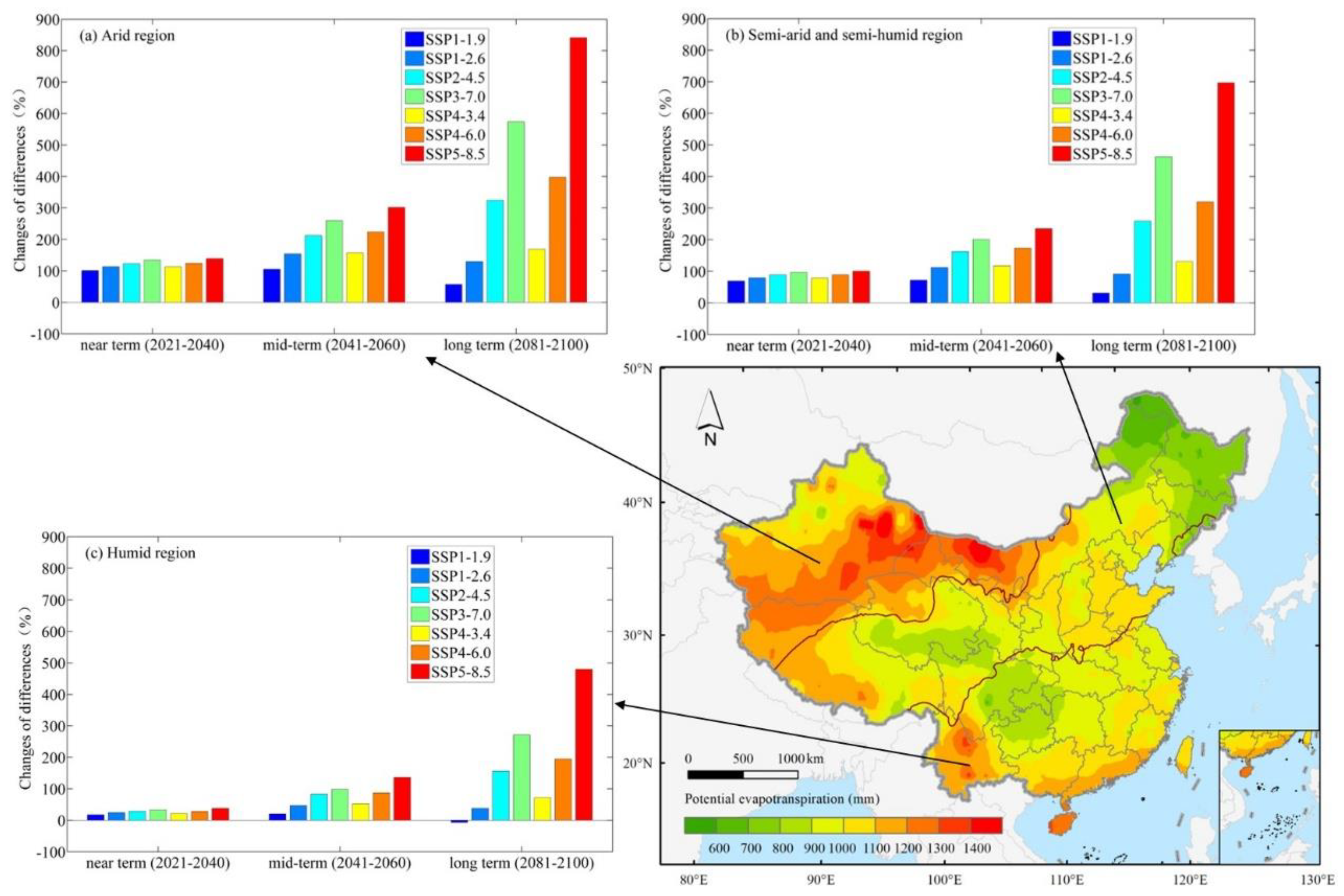
As shown in Figure 6, the spatial distribution of annual PET with the CO2 effect is above 600 mm in most areas of China for 1961–2014, and the amounts of PET are different among the climatic zones. In the arid region, the PET is relatively low in the northwest but high in the south and east, with values of about 900–1100 mm in the west and up to around 1200–1400 mm in the south and east. For the semi-arid and semi-humid region, the PET is approximately 800–1000 mm and is relatively lower in the northern part (approximately 600–800 mm) and relatively higher in the western and south-eastern parts with over 1000 mm. In the humid region, the PET is generally more than 900 mm, with values over 1200 mm in its southwestern and southern parts but just about 800 mm in its northwestern part.
In order to explore the changes in the differences between the two PET estimates for the three climatic zones under the SSPs in the near term (2021–2040), mid-term (2041–2060), and long term (2081–2100), the difference in PET computed by the two methods for China as a whole in 1995–2014, which is about 10 mm, is set as the baseline. Changes in differences relative to the baseline period are presented using the form of a bar chart in Figure 6.
For the arid region, the difference between PET without and with the CO2 effect increases by approximately 101–139% under different scenarios in the near term relative to the baseline period, with the smallest rise under SSP1-1.9 and the maximum increase under SSP5-8.5. During the mid-term, the difference will increase further. The smallest increase in the difference is about 105% under SSP1-1.9, and the maximum rise is approximately 302% under SSP5-8.5. In the long term, the increase in the difference is around 57% under SSP1-1.9, which is the only scenario in which the growth percentage is less than 100%. Under SSP1-2.6 and SSP4-3.4, the PET difference will increase by 130% and 169% compared with the baseline period. The PET difference will have massive expansion of 324%, 398%, 574% and 841% under SSP2-4.5, SSP4-6.0, SSP3-7.0, and SSP5-8.5, respectively.
In the semi-arid and semi-humid regions, the PET difference will increase by 69% to 101% under all scenarios during the near term relative to the baseline period. In the mid-term, the increase in the difference will be over 100%, except under SSP1-1.9, in which it is approximately 72%, and the maximum increase can up to 235% under SSP5-8.5. In the long term, the PET difference under SSP1-1.9 and SSP1-2.6 will increase by approximately 31% and 91% relative to the baseline period; under SSP4-3.4, the PET difference will increase by nearly 131%; and the difference of PET will be amplified by over 200% under SSP2-4.5, SSP4-6.0, SSP3-7.0 and SSP5-8.5 relative to the baseline period, with a maximum rise of 696% under SSP5-8.5.
In the humid region, the PET difference rises by 17% to 38% during the near term, with the smallest increase rate under SSP1-1.9 and the maximum increase under SSP5-8.5. In the mid-term, increasing rates of the PET difference is ranging from 20% to 136% under different scenarios relative to the baseline period, with the increase rates being relatively high under SSP3-7.0 and SSP5-8.5 by approximately 98% and 136%, respectively. Increases are less than 60% (approximately 20%, 47% and 53%, respectively) under SSP1-1.9, SSP1-2.6 and SSP4-3.4. The PET difference will rise by approximately 85% under the other scenarios. In the long term, the PET difference will decrease at a rate of 7% compared with the baseline period under SSP1-1.9. The difference between PET values increases by 38% to 195% under SSP1-2.6, SSP2-4.5, SSP4-3.4, and SSP4-6.0 relative to the baseline, but it is worth mentioning that although the difference under SSP1-2.6 increases compared to that of the baseline period, it is less than that in the mid-term. Under SSP3-7.0 and SSP5-8.5, the increasing PET difference is relatively high and reaches approximately 271% and 480%, respectively, relative to the baseline period, which is less than that in the arid region and the semi-arid and semi-humid region during the same period.
In general, the difference between estimated PET values with and without consideration of CO2 becomes increasingly high over time except under SSP1-1.9 and SSP1-2.6, and the increase in the difference is most pronounced in the arid region under SSP3-7.0 and SSP5-8.5.
3.3. Contribution Factors Analysis of PET
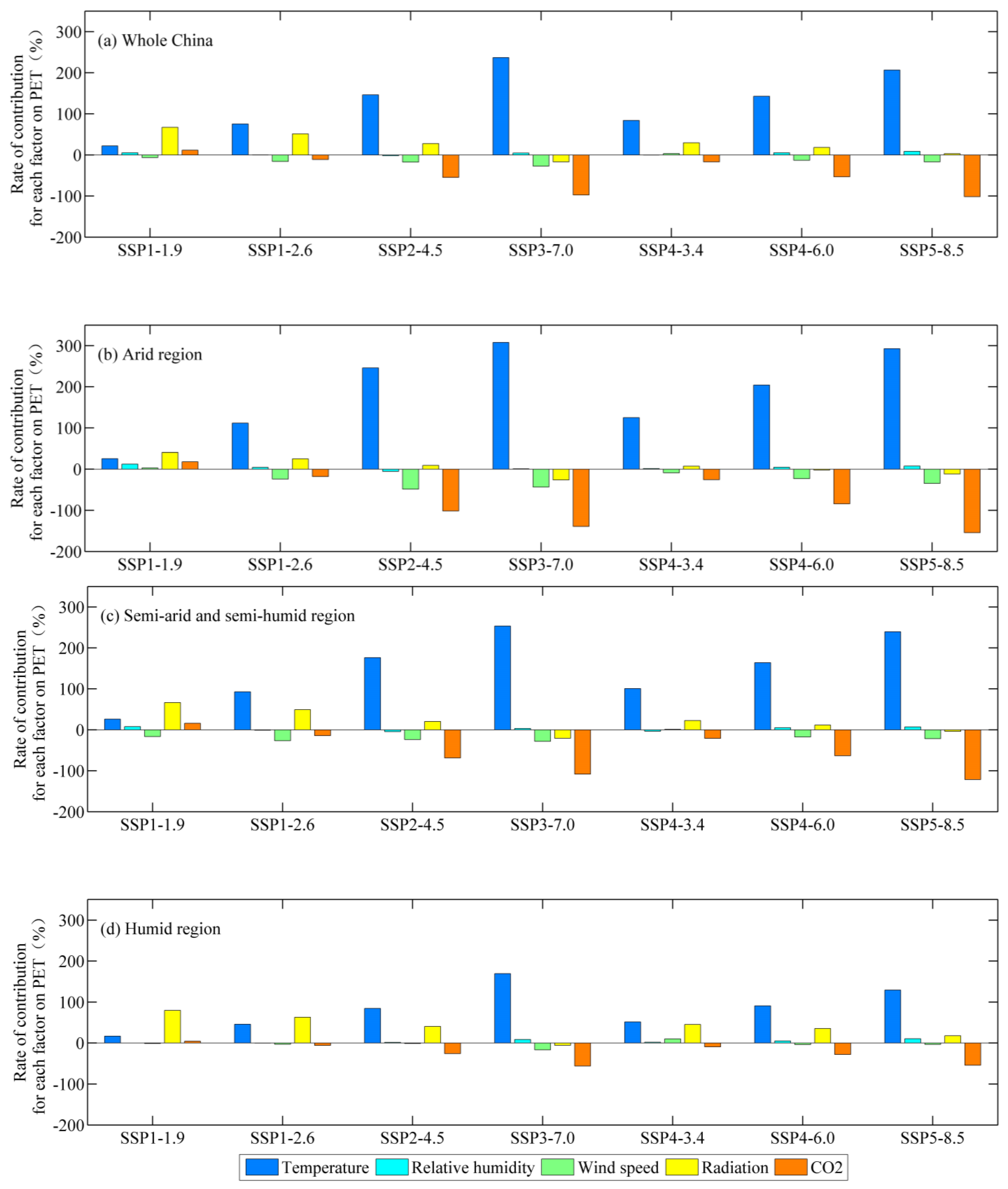
The contribution rate of each influential factor (temperature, relative humidity, wind speed, radiation, and CO2 concentration) to PET changes is further analyzed here as under the seven scenarios over entire China and its three climatic zones. As shown in Figure 7a, radiation is the most important factor affecting PET under SSP1-1.9 for the whole of China, which takes up the contribution rate by 67.3%. Contribution rates of temperature, CO2, relative humidity, and wind speed to PET are 22.1%, 11.5%, 5.3%, and −6.3%, respectively. Under other remaining scenarios, the temperature is the biggest contributor, but wind speed and CO2 are always playing the role of negative effects. Meanwhile, the negative effect of CO2 on PET strengthens with the increase of radiative forcing, the contribution rate of CO2 can reach −101.5% under SSP5-8.5. The negative contribution rate of wind speed is greater than −30%, which is smaller than the effect of CO2. Relative humidity and radiation have generally positive contributions to PET, the contribution rates are below 10% and 60%, respectively.
In arid region (Figure 7b), the contribution rates of factors are 40.5% (radiation), 25.7% (temperature), 18.1% (CO2), 12.4% (relative humidity), and 3.3% (wind speed) under SSP1-1.9. For other SSPs, the positive contribution of temperature to PET is highlighted, and the highest contribution rate is about 307.8% under SSP3-7.0. Relative humidity has a weak positive effect on PET and the rates of contribution are all not more than 10%. Radiation displays a positive effect on PET under low radiation forcing scenarios (SSP1-2.6, SSP2-4.5, and SSP4-3.4), but the negative effect on PET under high radiation forcing scenarios (SSP4-6.0, SSP3-7.0, and SSP5-8.5). Wind speed shows a negative effect on PET and the contribution rates are ranging from −48.4% to −8.7%. Compared with wind speed, the negative effect of CO2 is larger, the contribution rate of which can range −154.2% to −17.8%, which is lower than the China level under different scenarios.
For semi-arid and semi-humid regions (Figure 7c), the temperature is still the most important positive factor to PET except under SSP1-1.9 (the most important positive factor is radiation under SSP1-1.9), and the contribution rate can reach 253.5% under SSP3-7.0. Corresponding to this, CO2 is the most important negative factor to PET, and the contribution rate can range from −121.4% to −14.2% under different scenarios (the effect is smaller than that in the arid region). The contribution rates of relative humidity, wind speed, and radiation are quite smaller, and the biggest rates are about 7.7%, −28.1%, and 66.5%.
In humid region (Figure 7d), temperature and radiation are the main factors to PET under SSP1-1.9 (the contribution rates are 16.8% and 79.8%), SSP1-2.6 (46.1% and 63.1%), SSP2-4.5 (84.5% and 40.7%), SSP4-3.4 (51.7% and 45.3%) and SSP4-6.0 (90.8% and 35.5%). Only under high emission scenarios like SSP3-7.0 and SSP5-8.5, the negative contribution rate of CO2 to PET can over 50%. The contribution rates of relative humidity and wind speed are relatively lower, which are ranging from -16.5% to 10.6%. In summary, the effect of CO2 on PET in the humid region is not as important as that in other regions, especially in the arid region.
4. Conclusions and Discussion
A reasonable estimation of PET in the context of climate change is of great significance for water resources management. In this paper, seven global climate models are proved to have good simulation effects for the regional climate in China and are then used for PET estimation. The traditional PM method and modified PM method are compared to explore the effect of CO2 on PET estimation in a warming world in different climatic regions. The main conclusions are as follows:
(1) For China as a whole, the two types of PET show opposite trends in 1961–2014, decreasing with consideration of the effect of CO2 but increasing without CO2 effect. In 2015–2100, both PET series are projected to increase under all SSPs, with the trend estimated by the traditional PM method being higher than that estimated by the modified PM method. The PET difference first increases and then decreases under SSP1-1.9, SSP1-2.6, and SSP4-3.4; increases but slows down under SSP2-4.5 and SSP4-6.0; and continues to increase rapidly under SSP3-7.0 and SSP5-8.5. Temperature is the biggest contributor to PET generally, and wind speed and CO2 are always playing the role of negative effects. CO2 is the biggest negative effect on PET, and the effect strengthens with the increase of radiative forcing.
(2) In the arid region, both PET series increased during 1961–2014 and PET displays varying degrees of growth during 2015–2100 under the different scenarios. The difference between the two PET series shows an increasing trend slightly faster than the level of China as a whole. In the near term (2021–2040), the difference rises by approximately 101–139% under all scenarios relative to the baseline period (1995–2014). In the mid-term (2041–2060), the PET difference widens further, with a maximum of about 302% under SSP5-8.5. While in the long term (2081–2100), the increase in the difference will diminish under SSP1-1.9 but increase under SSP2-4.5, SSP4-6.0, SSP3-7.0, and SSP5-8.5. The negative contribution rates of CO2 to PET can range from −154.2% to −17.8% and this negative effect is greater than in other regions.
(3) In the semi-arid and semi-humid region, the changes in the PET difference over time are similar to those for China as a whole under all scenarios. The PET difference will increase under all scenarios during the three periods (near term, mid-term, and long term) compared to the baseline period, with a maximum of 696% under SSP5-8.5 in the long term. CO2 is also the most important negative factor to PET, but the effect is smaller than that in the arid region.
(4) In the humid region, PET values by two formulas decrease in 1961–2014 but increase in 2015–2100 under most scenarios, with the calculated PET increasing faster under the traditional method than when the CO2 effect is considered. The difference between the two PET series displays a weak upward trend in 1961–2014. In 2015–2100, the degree of increase is relatively less, and even the maximum difference under SSP3-7.0 and SSP5-8.5 is far less than that in the arid region. The effect of CO2 is relative not obvious, and only under high emission scenarios like SSP3-7.0 and SSP5-8.5, the negative contribution rate of CO2 to PET can be over 50%.
A previous study by Hua et al. (2020) [46] showed that the PM method significantly overestimates PET in the arid region by applying ground meteorological observations and various Moderate Resolution Imaging Spectroradiometer (MODIS) products for Northwest China. The results obtained in the current paper also prove that the traditional PM method overestimates PET. When a modified PM method that considers the CO2 effect is applied to estimate PET in China, it can be found that the PET amount is significantly reduced, and the difference between the two PET series will be amplified over time under most of the scenarios in the future. What is more, the greatest difference between the two PET series is found in the arid region spatially. The scarcity of plants, high altitude as well as the atmospheric uplift effect result in relatively high concentrations of CO2 in arid regions [47,48], and the high CO2 concentrations lead to a reduction in PET. Although the traditional PM formula fixes the characteristics of vegetation in the estimation of PET, it misses the response of vegetation to CO2 concentrations, resulting in the overestimation of PET. In other words, CO2 should be considered in PET estimation, as divergent PET estimates will lead to incorrect water resource projections and management decisions in arid regions. In this paper, the effect of CO2 on the physiological characteristics of vegetation is considered in the estimation of PET. However, there are some limitations in this paper. The PM formula by FAO, as the method which provides consistent PET values in all regions and climates, makes two assumptions when calculating potential evapotranspiration. Firstly, full evaporation is achieved under optimal soil moisture conditions and given climate conditions. Secondly, crop height of 0.12 m, a fixed surface resistance of 70 s m−1 and an albedo of 0.23, are as a reference surface for evaporation. Under such assumptions, the characteristics of assumed vegetation (vegetation types and cover densities) in the arid and humid regions are consistent in all aspects, that means it is not the actual vegetation. We mainly considered the influence of CO2 on the surface resistance parameter (rs), and calculated the PET under the unified standard vegetation cover. But the type, quantity and distribution density of vegetation may affect the potential evapotranspiration in the real world. Thus, many other factors, such as albedo and vegetation types, should be refined to consider in PET-related studies in the next step for a fast-changing world.
Author Contributions
T.J. and B.S. conceived the study. S.J. and J.Z. contributed to this paper by performing analyses and drafting the paper. C.J. calculated the PET covering the whole China. Y.W., J.H. and M.Z. integrated innovative ideas and improved the complete research and manuscript. All authors have read and agreed to the published version of the manuscript.
Funding
This research work was cooperatively funded by the National Key Research and Development Program of China MOST (2019YFC1510203), Key Research Program by Jiangxi Meteorological Bureau (JX201810) and the National Science Foundation of China (42105158, 42071024, 42005126). The authors are grateful to the program of the Innovative and Entrepreneurial Talents of Jiangsu Province, and the High-level Talent Re-cruitment Program of Nanjing University of Information Science and Technology (NUIST).
Institutional Review Board Statement
Not applicable.
Informed Consent Statement
Not applicable.
Data Availability Statement
The data used in this study are available from the corresponding author on reasonable request.
Acknowledgments
All the authors thank the World Climate Research Programme’s working group on coupled modeling for producing and making their model output available.
Conflicts of Interest
The authors declare that they have no known competing financial interests or personal relationships that could have appeared to influence the work reported in this paper.
References
- Darshana, P.A.; Pandey, R.P. Analysing trends in reference evapotranspiration and weather variables in the Tons River Basin in Central India. Stoch. Environ. Res. Risk Assess. 2013, 27, 1407–1421. [Google Scholar] [CrossRef]
- Hashem, A.A.; Engel, B.A.; Bralts, V.E.; Marek, G.W.; Moorhead, J.E.; Rashad, M.; Radwan, S.; Gowda, P.H. Landsat hourly evapotranspiration flux assessment using lysimeters for the texas high plains. Water 2020, 12, 1192. [Google Scholar] [CrossRef]
- Onyutha, C.; Acayo, G.; Nyende, J. Analyses of precipitation and evapotranspiration changes across the Lake Kyoga Basin in East Africa. Water 2020, 12, 1134. [Google Scholar] [CrossRef]
- Jung, M.; Reichstein, M.; Ciais, P.; Seneviratne, S.I.; Sheffield, J.; Goulden, M.L.; Bonan, G.; Cescatti, A.; Chen, J.Q.; Jeu, R.D.; et al. Recent decline in the global land evapotranspiration trend due to limited moisture supply. Nature 2010, 467, 951–954. [Google Scholar] [CrossRef]
- Tian, Y.; Zhang, K.J.; Xu, Y.P.; Gao, X.C.; Wang, J. Evaluation of potential evapotranspiration based on CMADS reanalysis dataset over China. Water 2018, 10, 1126. [Google Scholar] [CrossRef] [Green Version]
- Oki, T.; Kanae, S. Global hydrological cycles and world water resources. Science 2006, 313, 1068–1072. [Google Scholar] [CrossRef] [Green Version]
- Wang, K.C.; Dickinson, R.E. A review of global terrestrial evapotranspiration: Observation, modeling, climatology, and climatic variability. Rev. Geophys. 2012, 50. [Google Scholar] [CrossRef]
- Wild, M.; Folini, D.; Schär, C.; Loeb, N.; Dutton, E.G. The global energy balance from a surface perspective. Clim. Dyn. 2013, 40, 3107–3134. [Google Scholar] [CrossRef] [Green Version]
- Vicente-Serrano, S.M.; Azorin-Molina, C.; Sanchez-Lorenzo, A.; Revuelto, J.; López-Moreno, J.I.; González-Hidalgo, J.C.; Moran-Tejeda, E.; Espejo, F. Reference evapotranspiration variability and trends in Spain, 1961–2011. Glob. Planet Chang. 2014, 121, 26–40. [Google Scholar] [CrossRef] [Green Version]
- Milly, P.C.D.; Dunne, K.A. Potential evapotranspiration and continental drying. Nat. Clim. Chang. 2016, 6, 946–949. [Google Scholar] [CrossRef]
- Bai, P.; Liu, X.M.; Yang, T.T.; Li, F.D.; Liang, K.; Hu, S.S.; Liu, C.G. Assessment of the influences of different potential evapotranspiration inputs on the performance of monthly hydrological models under different climatic conditions. J. Hydrometeorol. 2016, 17, 2259–2274. [Google Scholar] [CrossRef]
- IPCC. 2021: Summary for Policymakers. In Climate Change 2021: The Physical Science Basis. Contribution of Working Group I to the Sixth Assessment Report of the Intergovernmental Panel on Climate Change; Masson-Delmotte, V.P., Zhai, A., Pirani, S.L., Connors, C., Péan, S., Berger, N., Caud, Y., Chen, L., Goldfarb, M.I., Gomis, M., et al., Eds.; Cambridge University Press: Cambridge, UK, 2021. [Google Scholar]
- Gong, X.L.; Du, S.P.; Li, F.Y.; Ding, Y.B. Study on the spatial and temporal characteristics of mesoscale drought in China under future climate change scenarios. Water 2021, 13, 2761. [Google Scholar] [CrossRef]
- Mondal, S.K.; Huang, J.L.; Wang, Y.J.; Su, B.D.; Zhai, J.Q.; Tao, H.; Wang, G.J.; Fischer, T.; Wen, S.S.; Jiang, T. Doubling of the population exposed to drought over South Asia: CMIP6 multi-model-based analysis. Sci. Total Environ. 2021, 771, 145186. [Google Scholar] [CrossRef] [PubMed]
- Shi, L.J.; Feng, P.Y.; Wang, B.; Liu, D.L.; Cleverly, J.; Fang, Q.X.; Yu, Q. Projecting potential evapotranspiration change and quantifying its uncertainty under future climate scenarios: A case study in southeastern Australia. J. Hydrol. 2020, 584, 124756. [Google Scholar] [CrossRef]
- Xiang, K.Y.; Li, Y.; Horton, R.; Feng, H. Similarity and difference of potential evapotranspiration and reference crop evapotranspiration—A review. Agric. Water Manag. 2020, 232, 106043. [Google Scholar] [CrossRef]
- Zhou, J.; Wang, Y.J.; Su, B.D.; Wang, A.Q.; Tao, H.; Zhai, J.Q.; Kundzewicz, Z.W.; Jiang, T. Choice of potential evapotranspiration formulas influences drought assessment: A case study in China. Atmos. Res. 2020, 242, 104979. [Google Scholar] [CrossRef]
- Allen, R.G.; Pereira, L.S.; Raes, D.; Smith, M. Crop Evapotranspiration: Guidelines for Computing Crop Water Requirements; FAO Irrigation and Drainage Paper 56; FAO: Rome, Italy, 1998; Available online: http://www.fao.org/docrep/X0490E/X0490E00.htm (accessed on 9 February 2022).
- Kim, K.; Daly, E.J.; Flesch, T.K.; Coates, T.W. Carbon and water dynamics of a perennial versus an annual grain crop in temperate agroecosystems. Agric. For. Meteorol. 2022, 314, 108805. [Google Scholar] [CrossRef]
- Yang, Y.T.; Roderick, M.L.; Zhang, S.L.; McVicar, T.R.; Donohue, R.J. Hydrologic implications of vegetation response to elevated CO2 in climate projections. Nat. Clim. Chang. 2019, 9, 44–49. [Google Scholar] [CrossRef]
- Yang, Y.T.; Zhang, S.L.; Roderick, M.; McVicar, T.R.; Yang, D.W.; Liu, W.B.; Li, X.Y. Comparing Palmer Drought Severity Index drought assessments using the traditional offline approach with direct climate model outputs. Hydrol. Earth Syst. Sci. 2020, 24, 2921–2930. [Google Scholar] [CrossRef]
- Zhang, G.X.; Su, X.L.; Liu, W.F. Future drought trend in China considering CO2 concentration. Trans. Chin. Soc. Agric. Eng. 2021, 37, 84–91. (In Chinese) [Google Scholar] [CrossRef]
- Field, C.B.; Jackson, R.B.; Mooney, H.A. Stomatal responses to increased CO2: Implications from the plant to the global scale. Plant Cell Environ. 1995, 18, 1214–1225. [Google Scholar] [CrossRef]
- Novick, K.A.; Ficklin, D.L.; Stoy, P.C.; Williams, C.A.; Bohrer, G.; Oishi, A.C.; Papuga, S.A.; Blanken, P.D.; Noormets, A.; Sulman, B.N.; et al. The increasing importance of atmospheric demand for ecosystem water and carbon fluxes. Nat. Clim. Chang. 2016, 6, 1023–1027. [Google Scholar] [CrossRef] [Green Version]
- Swann, A.L.S.; Hoffman, F.M.; Koven, C.D.; Randerson, J.T. Plant responses to increasing CO2 reduce estimates of climate impacts on drought severity. Proc. Natl. Acad. Sci. USA 2016, 113, 10019–10024. [Google Scholar] [CrossRef] [PubMed] [Green Version]
- Yang, Y.T.; Zhang, S.L.; McVicar, T.R.; Beck, H.E.; Zhang, Y.Q.; Liu, B. Disconnection Between Trends of Atmospheric Drying and Continental Runoff. Water Resour. Res. 2018, 54, 4700–4713. [Google Scholar] [CrossRef]
- Thompson, J.R.; Green, A.J.; Kingston, D.G. Potential evapotranspiration-related uncertainty in climate change impacts on river flow: An assessment for the Mekong River basin. J. Hydrol. 2014, 510, 259–279. [Google Scholar] [CrossRef] [Green Version]
- Giménez, P.O.; García-Galiano, S.G. Assessing regional climate models (RCMs) ensemble-driven reference evapotranspiration over Spain. Water 2018, 10, 1181. [Google Scholar] [CrossRef] [Green Version]
- Han, J.Y.; Zhao, Y.; Wang, J.H.; Zhang, B.; Zhu, Y.N.; Jiang, S.; Wang, L.Z. Effects of different land use types on potential evapotranspiration in the Beijing-Tianjin-Hebei region, North China. J. Geogr. Sci. 2019, 29, 922–934. [Google Scholar] [CrossRef] [Green Version]
- Duhan, D.; Singh, D.; Arya, S. Effect of projected climate change on potential evapotranspiration in the semiarid region of central India. J. Water Clim. Chang. 2020, 12, 1854–1870. [Google Scholar] [CrossRef]
- Shi, L.J.; Feng, P.Y.; Wang, B.; Liu, D.L.; Yu, Q. Quantifying future drought change and associated uncertainty in southeastern Australia with multiple potential evapotranspiration models. J. Hydrol. 2020, 590, 125394. [Google Scholar] [CrossRef]
- Wen, X.H.; Pan, W.Q.; Sun, X.G.; Li, M.S.; Luo, S.Q.; Cao, B.J.; Zhang, S.B.; Wang, C.; Zhang, Z.H.; Meng, L.X.; et al. Study on the Variation Trend of Potential Evapotranspiration in the Three-River Headwaters Region in China Over the Past 20 years. Front. Earth Sci. 2020, 448. [Google Scholar] [CrossRef]
- Yang, Y.; Chen, R.S.; Han, C.T.; Liu, Z.W. Evaluation of 18 models for calculating potential evapotranspiration in different climatic zones of China. Agric. Water Manag. 2021, 244, 106545. [Google Scholar] [CrossRef]
- Mondal, S.K.; Tao, H.; Huang, J.L.; Wang, Y.J.; Su, B.D.; Zhai, J.Q.; Jing, C.; Wen, S.S.; Jiang, S.; Chen, Z.Y.; et al. Projected changes in temperature, precipitation and potential evapotranspiration across Indus River Basin at 1.5–3.0 °C warming levels using CMIP6-GCMs. Sci. Total Environ. 2021, 789, 147867. [Google Scholar] [CrossRef] [PubMed]
- Yang, Y.; Chen, R.S.; Song, Y.X.; Han, C.T.; Liu, J.F.; Liu, Z.W. Sensitivity of potential evapotranspiration to meteorological factors and their elevational gradients in the Qilian Mountains, northwestern China. J. Hydrol. 2019, 568, 147–159. [Google Scholar] [CrossRef]
- Zhang, X.L.; Xiao, W.H.; Wang, Y.C.; Wang, Y.; Kang, M.Y.; Wang, H.J.; Huang, Y. Sensitivity analysis of potential evapotranspiration to key climatic factors in the Shiyang River Basin. J. Water Clim. Chang. 2021, 12, 2875–2884. [Google Scholar] [CrossRef]
- Tang, Y.; Tang, Q.H. Variations and influencing factors of potential evapotranspiration in large Siberian river basins during 1975–2014. J. Hydrol. 2021, 598, 126443. [Google Scholar] [CrossRef]
- Su, B.D.; Huang, J.L.; Mondal, S.K.; Zhai, J.Q.; Wang, Y.J.; Wen, S.S.; Gao, M.N.; Lv, Y.R.; Jiang, S.; Jiang, T.; et al. Insight from CMIP6 SSP-RCP scenarios for future drought characteristics in China. Atmos. Res. 2020, 250, 105375. [Google Scholar] [CrossRef]
- Su, B.D.; Huang, J.L.; Gemmer, M.; Jian, D.N.; Tao, H.; Jiang, T.; Zhao, C.Y. Statistical downscaling of CMIP5 multi-model ensemble for projected changes of climate in the Indus River Basin. Atmos. Res. 2016, 178–179, 138–149. [Google Scholar] [CrossRef]
- Su, B.D.; Huang, J.L.; Fischer, T.; Wang, Y.J.; Kundzewicz, Z.W.; Zhai, J.Q.; Sun, H.M.; Wang, A.Q.; Zeng, X.F.; Wang, G.J.; et al. Drought losses in China might double between the 1.5 °C and 2.0 °C warming. Proc. Natl. Acad. Sci. USA 2018, 115, 10600–10605. [Google Scholar] [CrossRef] [Green Version]
- Meinshausen, M.; Vogel, E.; Nauels, A.; Lorbacher, K.; Meinshausen, N.; Etheridge, D.M.; Fraser, P.J.; Montzka, S.A.; Rayner, P.J.; Trudinger, C.M.; et al. Historical greenhouse gas concentrations for climate modelling (CMIP6). Geosci. Model Dev. 2017, 10, 2057–2116. [Google Scholar] [CrossRef] [Green Version]
- Meinshausen, M.; Nicholls, Z.R.J.; Lewis, J.; Gidden, M.J.; Vogel, E.; Freund, M.; Beyerle, U.; Gessner, C.; Nauels, A.; Bauer, N.; et al. The shared socio-economic pathway (SSP) greenhouse gas concentrations and their extensions to 2500. Geosci. Model Dev. 2020, 13, 3571–3605. [Google Scholar] [CrossRef]
- Sun, S.L.; Chen, H.S.; Sun, G.; Ju, W.M.; Wang, G.J.; Li, X.; Yan, G.X.; Gao, C.J.; Huang, J.; Zhang, F.M.; et al. Attributing the changes in reference evapotranspiration in Southwestern China using a new separation method. J. Hydrometeorol. 2017, 18, 777–798. [Google Scholar] [CrossRef]
- Wild, M.; Gilgen, H.; Roesch, A.; Ohmura, A.; Long, C.N.; Dutton, E.G.; Forgan, B.; Kallis, A.; Russak, V.; Tsvetkov, A. From dimming to brightening: Decadal changes in solar radiation at earth’s surface. Science 2005, 308, 847–850. [Google Scholar] [CrossRef] [PubMed] [Green Version]
- Yin, Y.H.; Wu, S.H.; Dai, E.F. Determining factors in potential evapotranspiration changes over China in the period 1971–2008. Chin. Sci. Bull. 2010, 55, 2226–2234. (In Chinese) [Google Scholar] [CrossRef]
- Hua, D.; Hao, X.M.; Zhang, Y.; Qin, J.X. Uncertainty assessment of potential evapotranspiration in arid areas, as estimated by the Penman-Monteith method. J. Arid. Land 2020, 12, 166–180. [Google Scholar] [CrossRef] [Green Version]
- Dai, L.J.; Cui, W.H.; Jiang, Y.B. Temporal and spatial distribution of tropospheric carbon dioxide from 2003 to 2010 in China. Ecol. Environ. Sci. 2012, 21, 1266–1270. (In Chinese) [Google Scholar] [CrossRef]
- Bai, W.G.; Zhang, X.Y.; Zhang, P. Temporal and spatial distribution of tropospheric CO2 over China based on satellite observations. Chin. Sci. Bull. 2010, 55, 3612–3618. [Google Scholar] [CrossRef]
Figure 1.
Spatial distribution of meteorological grids and three climatic regions in China: (a) arid region, (b) semi-arid and semi-humid region, and (c) humid region (red curves are the boundary between different climatic zones).
Figure 1.
Spatial distribution of meteorological grids and three climatic regions in China: (a) arid region, (b) semi-arid and semi-humid region, and (c) humid region (red curves are the boundary between different climatic zones).

Figure 2.
Changes in CO2 concentration in China from 1961 to 2100.

Figure 3.
Comparison of the ensemble mean of GCMs’ simulated and observed monthly mean temperature (a) and monthly precipitation (b) in China for 1961–2014. Note: The upper and lower limits represent the range of climate models.
Figure 3.
Comparison of the ensemble mean of GCMs’ simulated and observed monthly mean temperature (a) and monthly precipitation (b) in China for 1961–2014. Note: The upper and lower limits represent the range of climate models.

Figure 4.
Spatial distribution of annual mean temperature (a,b) and annual precipitation (c,d) based on observation and the multi-model ensemble mean for 1961–2014. The left column is observation and the right column is simulated values.
Figure 4.
Spatial distribution of annual mean temperature (a,b) and annual precipitation (c,d) based on observation and the multi-model ensemble mean for 1961–2014. The left column is observation and the right column is simulated values.

Figure 5.
The differences between PET estimations with and without the CO2 effect for 1961–2100: China (a); the arid region (b); the semi-arid and semi-humid region (c); and the humid region (d).
Figure 5.
The differences between PET estimations with and without the CO2 effect for 1961–2100: China (a); the arid region (b); the semi-arid and semi-humid region (c); and the humid region (d).

Figure 6.
Spatial distribution of annual mean PET with CO2 for 1961–2014 and its future change in the three climatic zones in China.
Figure 6.
Spatial distribution of annual mean PET with CO2 for 1961–2014 and its future change in the three climatic zones in China.

Figure 7.
Contribution rates of each factor on PET under different kinds of SSPs from 2015 to 2100: China (a); arid region (b); semi-arid and semi-humid region (c); humid region (d).
Figure 7.
Contribution rates of each factor on PET under different kinds of SSPs from 2015 to 2100: China (a); arid region (b); semi-arid and semi-humid region (c); humid region (d).


Table 1.
Basic information on the seven GCMs used in this paper.
| Model Name | Research Institution | Original Resolution |
|---|---|---|
| CanESM5 | Canadian Centre for Climate Modeling and Analysis | ~2.8° × 2.8° |
| CNRM-ESM2-1 | Centre National de Recherches Météorologiques- Centre Européen de Recherche et de Formation Avancée en Calcul Scientifique (CNRM-CERFACS) | 1.4° × 1.4° |
| FGOALS-g3 | Chinese Academy of Sciences (CAS) | 2.3° × 2° |
| GISS-E2-1-G | Goddard Institute for Space Studies (NASA-GISS) | 2° × 2.5° |
| IPSL-CM6A-LR | Institut Pierre-Simon Laplace | 2.5° × ~1.27° |
| MIROC6 | AORI-UT-JAMSTEC-NIES | ~1.4° × 1.4° |
| MRI-ESM2-0 | Meteorological Research Institute Earth System | ~1.125° × 1.12° |
Table 2.
Trends of annual PET in China and the three climatic zones for 1961–2014 and 2015–2100 under the seven SSPs (unit: mm/10a).
Table 2.
Trends of annual PET in China and the three climatic zones for 1961–2014 and 2015–2100 under the seven SSPs (unit: mm/10a).
| China | Arid Region | Semi-Arid and Semi-Humid Region | Humid Region | |||||
|---|---|---|---|---|---|---|---|---|
| Y | N | Y | N | Y | N | Y | N | |
| 1961–2014 | −0.4 | 1.1 | 1.2 | 3.6 | 0.7 | 2.8 | −4.0 | −2.7 |
| SSP1-1.9 | 3.4 | 3.0 | 2.8 | 2.3 | 2.6 | 2.2 | 5.5 | 5.2 |
| SSP1-2.6 | 4.3 | 4.7 | 3.1 | 3.6 | 3.3 | 3.8 | 7.0 | 7.4 |
| SSP2-4.5 | 5.4 | 8.2 | 3.4 | 6.9 | 4.4 | 7.3 | 8.9 | 11.0 |
| SSP3-7.0 | 5.9 | 11.6 | 5.1 | 12.3 | 5.5 | 11.5 | 7.3 | 11.2 |
| SSP4-3.4 | 6.4 | 7.4 | 4.7 | 5.9 | 5.0 | 6.1 | 10.3 | 11.2 |
| SSP4-6.0 | 7.1 | 10.8 | 5.4 | 10.0 | 6.1 | 10.0 | 10.4 | 13.1 |
| SSP5-8.5 | 9.1 | 18.4 | 7.3 | 18.5 | 7.7 | 17.2 | 13.3 | 20.4 |
Note: Y and N represent the CO2 effect and without the CO2 effect, respectively.
Publisher’s Note: MDPI stays neutral with regard to jurisdictional claims in published maps and institutional affiliations. |
© 2022 by the authors. Licensee MDPI, Basel, Switzerland. This article is an open access article distributed under the terms and conditions of the Creative Commons Attribution (CC BY) license (https://creativecommons.org/licenses/by/4.0/).
Share and Cite
MDPI and ACS Style
Zhou, J.; Jiang, S.; Su, B.; Huang, J.; Wang, Y.; Zhan, M.; Jing, C.; Jiang, T. Why the Effect of CO2 on Potential Evapotranspiration Estimation Should Be Considered in Future Climate. Water 2022, 14, 986. https://doi.org/10.3390/w14060986
AMA Style
Zhou J, Jiang S, Su B, Huang J, Wang Y, Zhan M, Jing C, Jiang T. Why the Effect of CO2 on Potential Evapotranspiration Estimation Should Be Considered in Future Climate. Water. 2022; 14(6):986. https://doi.org/10.3390/w14060986
Chicago/Turabian StyleZhou, Jian, Shan Jiang, Buda Su, Jinlong Huang, Yanjun Wang, Mingjin Zhan, Cheng Jing, and Tong Jiang. 2022. "Why the Effect of CO2 on Potential Evapotranspiration Estimation Should Be Considered in Future Climate" Water 14, no. 6: 986. https://doi.org/10.3390/w14060986
Note that from the first issue of 2016, this journal uses article numbers instead of page numbers. See further details here.