
Physical Experimentation and 2D-CFD Parametric Study of Flow through Transverse Bottom Racks


1
Department of Civil Engineering, Universidad Técnica Particular de Loja (UTPL), Loja 1101608, Ecuador
2
Esc. Ing. Caminos, Campus Fuentenueva, University of Granada, 18071 Granada, Spain
*
Author to whom correspondence should be addressed.
Water 2022, 14(6), 955; https://doi.org/10.3390/w14060955
Submission received: 24 February 2022
/
Revised: 11 March 2022
/
Accepted: 14 March 2022
/
Published: 18 March 2022
(This article belongs to the Section Hydraulics and Hydrodynamics)
Abstract
:In the present study, the hydraulic operation of flow through transverse bottom racks screens with conventional triangular wedge wire and alternative circular section wire is experimentally and numerically analyzed. A laboratory prototype is built for experimentation with clean water and sediment. The numerical experiment is developed with the Ansys Fluent software, and a 2D CFD parametric study is designed to evaluate the influence on the captured flow of geometric variables, such as the screen incline, position of the screen along the channel (top, middle, bottom), and shape, wire width, or slot width. The physical model results make it possible to determine the efficiency of the screens in terms of collection capacity and sediment removal. In contrast, numerical experimentation determines the influence of geometric variables on the collection flow. The flows captured by each screen slot are determined numerically. The trends of the total flows captured are determined, and the performance of each studied screen type is assessed using the relevant non-dimensional parameters.
1. Introduction
Surface water intake with bottom racks is one of the most used methods, especially in mountain rivers with steep slopes and irregular beds with significant sediment transport and flood flows. The screens are designed to capture as much water as possible while preventing the entry of as many solids as possible.
Concerning the direction of flow, the bars that compose a bottom rack can be parallel or perpendicular, and the cross-section of the bars is generally rectangular or circular. However, bars with various geometric shapes are also used. As it is a relevant structure within the field of Hydraulic Engineering, the problem of correctly designing the minimum area necessary to derive the required flow and remove as much sediment as possible has attracted the attention of several researchers who have investigated the problem both theoretically and experimentally.
For the most part, research referring to intakes with bottom racks has focused on racks formed by bars arranged parallel to the direction of flow. There is abundant technical literature regarding their calculation and design procedures. Consequently, they are more commonly used [1,2,3]. Detailed studies on horizontal transverse bottom racks are limited in the technical literature.
All types of water intake need separation from the water of waste, fish, sediment, and other materials. In recent years, the demand for effectively separating debris has risen with the need for more optimum removal. Modern irrigation systems (e.g., drip, sprinklers, valves, pumps) need a finer scale of material removal than conventional flood irrigation. Fish, sediment, and fine debris removal for small-scale water intake projects are required in distant areas. These structures combine high-capacity screening, self-cleaning hydraulic performance, and fine debris removal, all powered by gravity and without the need for electricity, as described by [4].
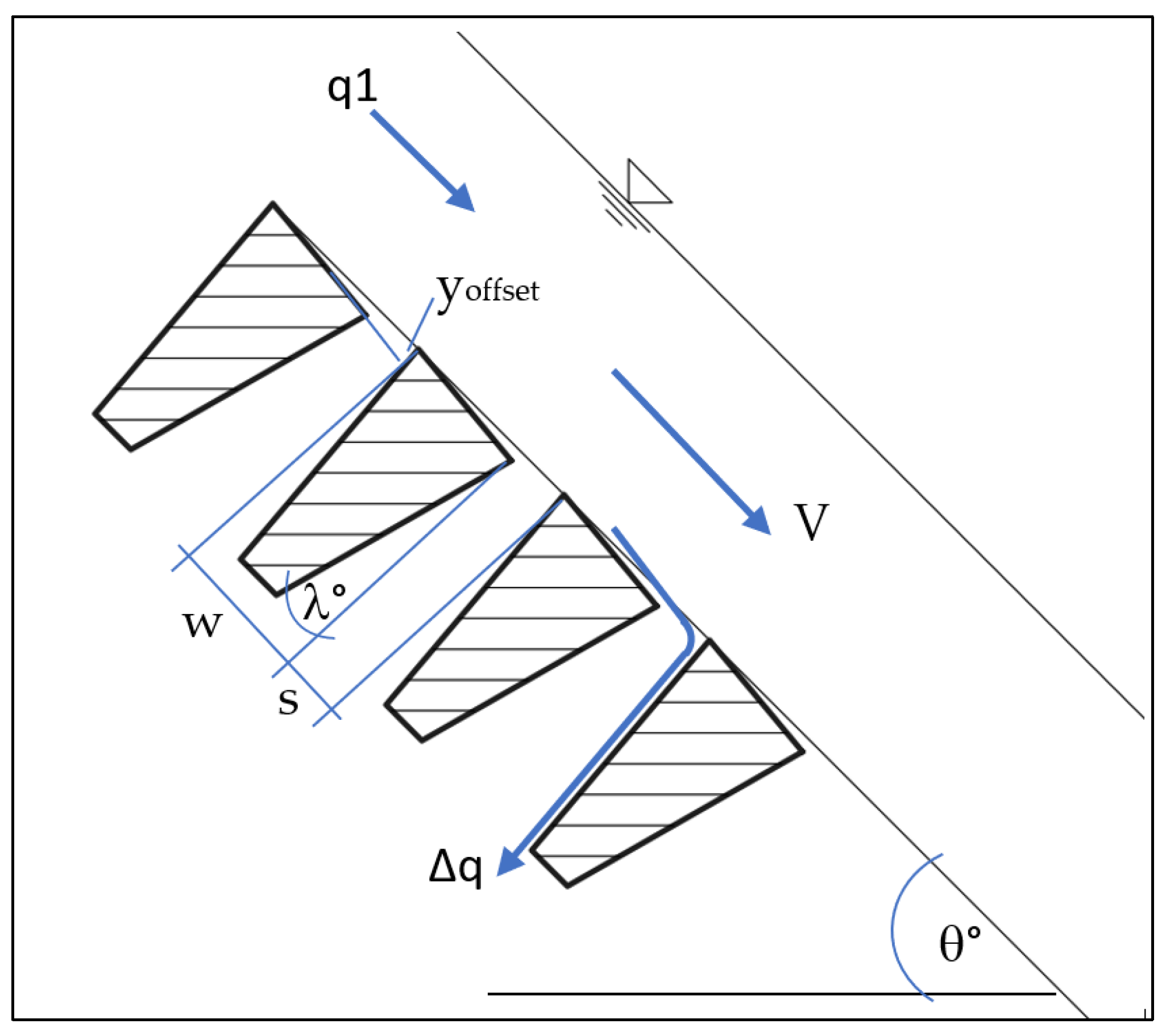
Many of the screening difficulties are solved using Coanda-effect screens. Since the 1980s, Coanda-effect screens have been used to screen organic waste, garbage, silt, and aquatic organisms from various water intakes [5,6]. The operation of the screens consists of the separation of solids present in a supercritical water flow that passes over wedge-shaped wires arranged perpendicular to the direction of the flow. Figure 1 is a schematic representation of a typical Coanda-effect screen structure.
As they are patented structures, the manufacture of Coanda-effect screen structures is purely industrial, and the commercial availability is limited [5,6]. For the correct hydraulic operation, the geometric variables of the wires must be constructed with great precision, especially the separation and angular offset, which is why manual manufacture is very complex and relatively expensive. Conventional surface water intake systems generally use bars of regular sections (circular, square) that are arranged parallel to the flow. These types of bars have high commercial availability.
For practical purposes and ease of construction, an alternative Coanda screen with circular section wires as proposed, especially for small water intakes in rural populations of less than 1000 inhabitants. Consequently, the hydraulic operation of a conventional Coanda-effect screen (wedge wire) and a Coanda screen with circular wires were experimentally and numerically evaluated with similar wire widths and spacing. Physical experimentation was performed with clean water and with the presence of sediments. The hydraulic prototype consisted of a rectangular channel that allowed variations of inclination. The tests were carried out with a flow rate of 2.5 L/s and angles of inclination of the rectangular channel of 20°, 35°, and 45°. In the physical tests, the flow results were total because it was not possible to measure the flow captured by each slot. The experimental tests with clean water showed that the triangular section wire screen was more efficient in the flow captured. However, the circular wire screens showed greater efficiency in removing solids in water with sediment.
In a second scenario, to determine the flow of clean water captured by each slot in the screen, as well as its velocity and pressure, the configuration and calibration of a 2D numerical model were carried out from the result of a test of the A-5 prototype analyzed by [4]. Once the numerical model was calibrated, a parametric study was conducted to evaluate the effect on the captured flow of modification of the wire section, screen inclination, position along the channel (top, middle, bottom), and slot size. Hence, this study makes it possible to determine the flow trend captured in total and in each slot of the Coanda-effect screen.
The 2D CFD parametric study was carried out with the numerical code Ansys Fluent 2020 R1 academic version [7].
Background
The literature provides limited details about research on horizontally transverse bottom racks. The review described below specifically reports studies of the physical and numerical experimentation of bottom bars transverse to the flow, with clean water and with the presence of sediment.
Channels with moderate or no slopes are the most often used in this area of research. Bouvard [8], Kuntzmann and Bouvard [9], and Mostkow [10] developed numerous hypotheses and formulae relating the quantity of flow, its depth, and the length of racks. Different bars with semicircular and triangular tops were studied by Jain et al. [11], who surveyed how the ratio of diverted flow to upstream flow changed as the bars’ angle changed. Ranga Raju et al. [12] analyzed the flow through transverse bottom racks with circular bars. They observed that the specific energy along a transverse bottom rack decreased along with the rack. Subramanya et al. [13], in their work on the hydraulic operation of transverse bottom racks, noticed that the value of the discharge coefficient C was not constant but varied with the flow and parameters of the rack geometry. Wahl and Einhellig [14] developed a numerical model using the spatially varied flow equation with decreased discharge to determine the flow rate through a Coanda-effect screen and the variation of its capture capacity based on the geometric parameters of the screen. The studied parameters were the drop height, wire width, wire separation, wire tilt angle, screen tilt, and Froude number of the flow passing over the screen. For the elaboration of the model and its calibration, the data came from several types of Coanda-effect screens with different configurations used in the laboratory to evaluate their hydraulic performance. Wahl [15] presented a computational model to calculate the hydraulic performance of Coanda-effect displays. Using laboratory tests with clean water, he evaluated the discharge characteristics of various screen types. He proposed a relationship to calculate the discharge based on the Froude number, specific energy, Reynolds number, and Weber number.
Ojha et al. [16] confirmed the dependence of the discharge coefficient on the flow and parameters of the screen geometry, such as the Froude number, porosity, and relationship of the width of the bar to the length of the frame through laboratory tests of flows on horizontal grids submerged transversely to the flow. Esmond [17] evaluated a Coanda-effect screen with separation between 0.5 mm wires in a test rainwater sink in Rowlett, Texas, between June 2009 and March 2011. During this period, an amount of 25,500 kg/km2/year of urban waste and sediments, which passed over the screen without entering, it was recorded. Of the urban waste and sediments that passed over the screen, 40% comprised particles between 0.5 mm and 5 mm, and 60% comprised particles greater than 5 mm of mainly grass and debris. The work concludes that the Coanda-effect screen removes many metals and other contaminants that impair water quality. In addition, the unit did not require maintenance during its operation. The Coanda-effect screen provides the following detailed removal information: debris and sediments 67%, arsenic 47%, cadmium 100%, copper 33%, nickel 39%, zinc 33%, and fecal coliforms 35%.
May [18], through laboratory studies, evaluated the efficiency of Coanda-effect screens to exclude sediments and performed tests for both clean water and sediment-laden flow. Sediment removal rates ranged from 43% to 81%, and the capture flow reduction due to obstruction reached a maximum value of 55%. The amount of flow through a screen and the ability to exclude sediment were inversely related.
Wahl [19] conducted laboratory tests with Coanda-effect screens with a more comprehensive flow range than initially planned. New experiments were developed with various screen types in an adjustable slope channel, from almost horizontal to an inclination of more than 50 degrees. The new tests showed that screen capability is a Froude number and Weber number complex functions. It was shown that the Reynolds number does not significantly affect the flow capacity of the screen.
Numerical studies by Seong-Min Yun et al. [20] were conducted for the optimal design of the dust separator screen using the Coanda-effect. The study evaluates the effect of the right curvature radius at the top of the dust separator screen and the left curvature radius at the top. In addition to the physical experiments, width ratio effects were studied with computational fluid dynamics (CFD) modeling. Finally, Wahl [4] studied the surface tension effects on the discharge capacity of Coanda-effect screens and tested small sections of prototype-scale screens at varying slopes, verifying that discharge coefficients are related to Froude and Weber numbers.
This paper is organized as follows. The second section describes the procedure used for the development of physical experimentation and numerical experimentation, and a summary of the cases analyzed is presented. The third section is dedicated to the analysis and discussion of the results. Finally, some conclusions are reported.
2. Materials and Methods
2.1. Physical Experimentation
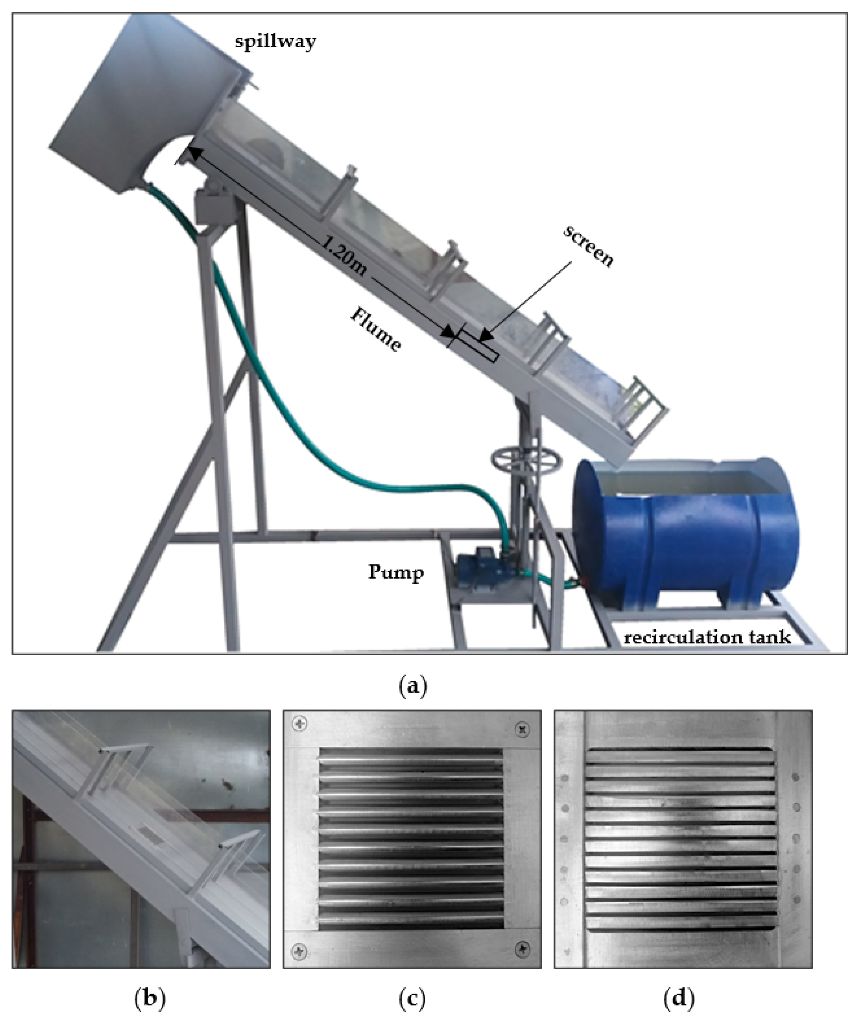
The physical experimentation was developed in a laboratory model composed of a 2 m-long and 9.3 cm-wide rectangular prismatic channel (Figure 2), with a range of angular variation from 20° to 45° concerning the horizontal.
The system has a cistern tank and a pump that recirculates the flow. The water is driven into an upper tank that has a weir through which the flow enters the rectangular channel and subsequently passes over the Coanda screen. The grid captures part of the flow, and another part returns to the cistern. The flow of water that enters the grid is collected in another tank for later measurement. The grate is located 1.2 m away from the upper edge of the channel. Tests were performed for both clean water and water with sediment.
The physical model has a funnel system that allows a valve to add a specific sediment load at the channel’s beginning. The tests were carried out at the channel’s 20°, 35°, and 45° inclination regarding the horizontal, a clean water flow of 2.5 L/s, and a sediment load of 25 gr/L. May [18] mentions that a 25 gr/L sediment load is approximately similar to the sediment load of a mountain river where this type of grating is used.
The water with sediment was separated from the recirculation system since the pump was not designed to work with particles. Hence, the water captured by the screen and the water that passed over it was collected in individual tanks for ensuing measurements.
Physical tests for both screens (triangular and circular section wire) were performed under the same flow, sediment load, channel location, inclination, width, and wire separation conditions. Table 1 details the geometric characteristics of each of the grids used.
The flows were obtained by the volumetric method. The efficiency of the grids was determined according to the flow rate captured and the volume of sediment removed. The sediment used was river sand. The selected particle sizes were those available in the series of sieves less than 2 mm, such as 1 mm, 0.3 mm, 0.15 mm, and 0.063 mm. Individual tests were carried out with each sediment size. For each test, a weight of 315 gr was poured, corresponding to the flow of 2.5 L/s and the sediment load of 25 gr/L.
2.2. Numerical Experimentation
Numerical modeling allows the computations of variables that are difficult to measure by experimental procedures. In particular, the model can calculate velocity and pressure in each screen slot. It is possible to study the effect generated by modifying independent variables such as the inclination, screen location along the channel, section, and separation of wires, etc., avoiding expensive modifications of the experimental setup.
Mathematical models still present precision problems when modeling some hydraulic phenomena [21,22]. Therefore, it is necessary to validate the numerical results with the data obtained in prototypes or physical models [23]. Laboratory measurements with clean water were used to validate CFD simulations. All calculations were performed using general-purpose code based on the finite volume method using Ansys Fluent [7].
The calibration of the numerical model was carried out using one of the laboratory results measured by Wahl [4] (screen A-5). Correspondingly, the code was validated with the laboratory results obtained in the physical model of the present study.
The procedure used for the development of numerical experimentation was as follows:
- Geometry construction
- Discretization
- Boundary conditions
- Configuring numerical simulation parameters
- Validation
- 2D parametric study
- Analysis of the results
2.2.1. Geometry
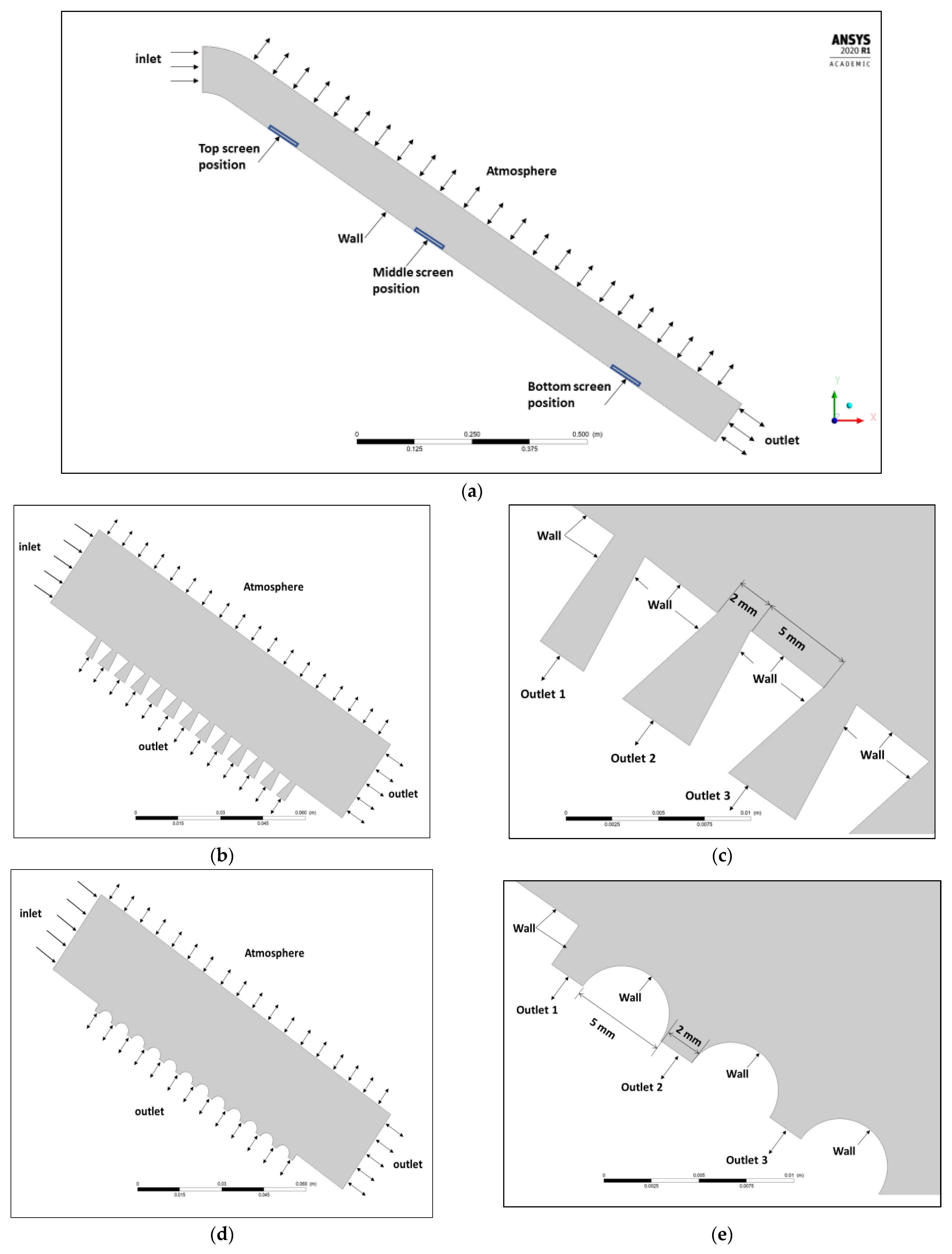
The geometry comprising the weir, channel, and grate was extracted from the physical model by Wahl [4], and the prototype of the physical model of the present investigation was extracted using aided design techniques. Figure 3 depicts the schematic of the domains for the current work. The first domain, shown in Figure 3a, comprises the weir and the channel; the second domain, Figure 3b,c, includes the triangular wire Coanda screen; and the third domain, Figure 3d,e, comprises the circular wire Coanda screen. The weir and channel domain were created to obtain a fully developed flow without interference from the screen. Once the flow profile stabilizes and converges, the velocity, pressure, and phase profiles perpendicular to the channel wall in any position can be obtained by interpolation. For the present study, profiles were generated in 3 zones, top, middle, and bottom, with load heights of 15, 35, and 70 cm, respectively. These heights were measured from the weir’s crest to the first screen slot. The domain of the spillway and channel was generated with three different angles, 20, 35, and 45 degrees. The domain of the screen used the information obtained in each channel profile. In this way, the hydraulic operation was evaluated as a function of velocity and water depth. Simultaneously, independent flow values were obtained for each opening.
2.2.2. Discretization
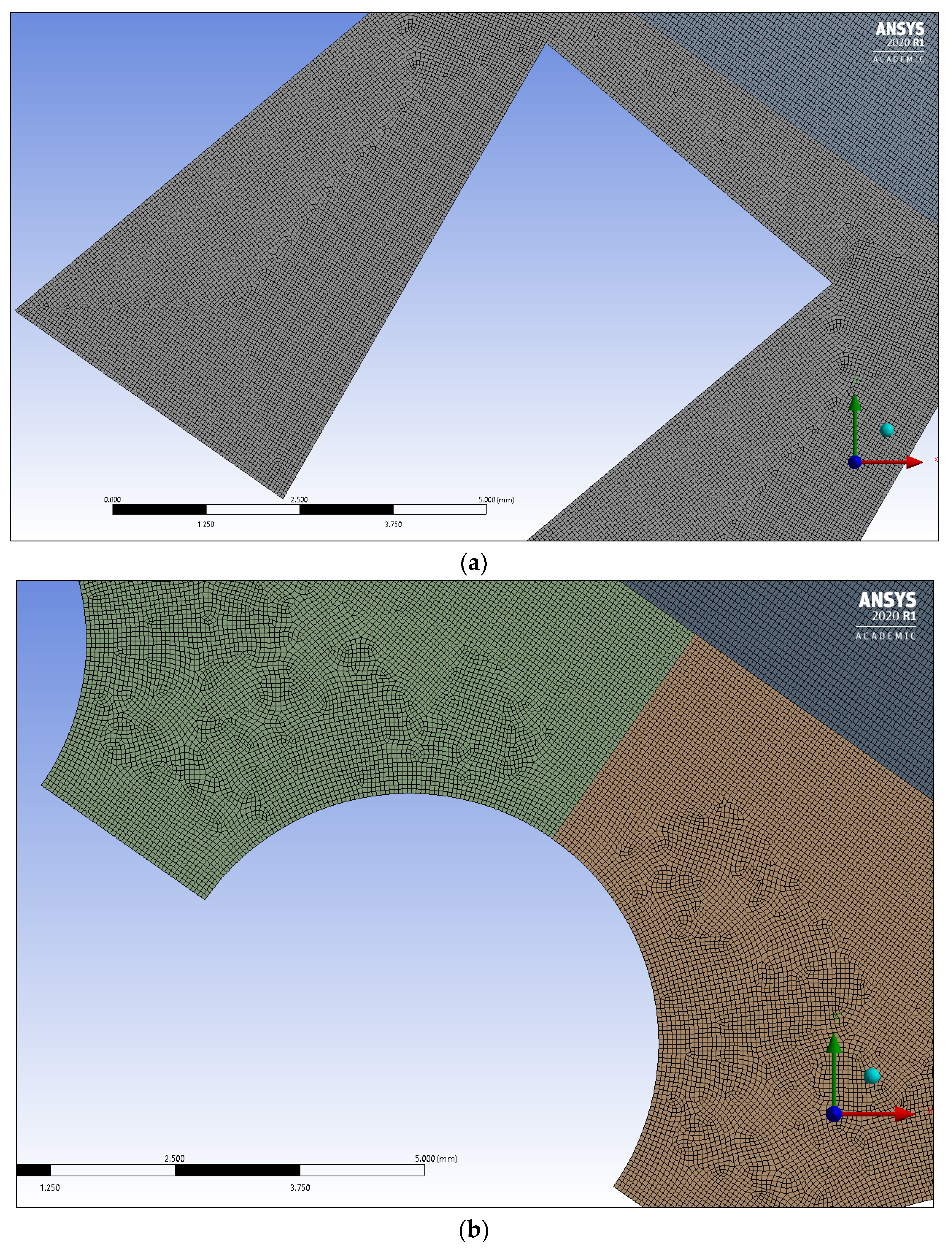
The grids were generated independently for each domain, while the calibration of the model was produced from a sensitivity analysis based on the independence of the mesh size. Refinement was carried out until the results of the flow captured by the grids were similar to those measured in the physical model. Quadrilateral elements were used with cell sizes ranging from 0.3 mm in the channel to 0.04 mm in the grids. The greatest refinement was carried out in the area of the wires. Figure 4a,b shows an example of a triangular and circular wire mesh, respectively. The wire width was 5 mm with a 2 mm separation, the total number of nodes was 671,511, the thickness of the first layer was 0.04 mm, and the maximum and minimum mesh size was 0.1 mm and 0.04 mm, respectively.
2.2.3. Computational Conditions
2.2.4. Numerical Resolution Method
The commercial CFD software ANSYS FLUENT 2020 R1 was applied for the numerical experimentation. The code uses a finite volume method [24] based on a second order of accuracy scheme to solve the transport equations for both laminar and turbulent models. The k–ωSST turbulence model [25] was adopted to close the equations. This model provides higher accuracy and reliability in the predicting flows near wall regions.
The complete equations of motion are presented in [7] (pages 2–4), while a detailed description of the turbulence models used has also been described in [7] (pages 65–67). For a report of the well-known Volume of fluid procedure, readers can refer to [7] (pages 558–560).
The coupled method [26] was used to handle the pressure-velocity coupling, resulting in more robust results and greater control over the stability and convergence behavior. The convergence criteria used in this study were based on a maximum residual of RES = 10−6 as a criterion for confirming convergence to a steady state with highly accurate solutions.
Table 4 presents a summary of the numerical schemes and solution methods used for numerical experimentation.
2.2.5. Validation
The numerical simulation was validated from one of the tests performed and provided by Wahl [4]. Table 5 presents a summary of the characteristics of the case used for the validation of the CFD model.
The geometric variables indicated in Table 5 were used to generate the geometry of the computational domains of the channel and the screen. The variables’ critical depth and inlet flow were used in the inlet condition of the channel. The flow rate captured corresponds to the six slots considered for the study. The flow rate value was used to compare the lab results with the CFD results. Once the simulation was validated, we computed and compared the flows of four cases tested in the experimental prototype: two triangular wire screens and two circular wire screens, respectively.
2.2.6. CFD Parametric Study
The influence on the captured flow rate of the modification of geometric variables of the channel and the screen was evaluated via a CFD-2D parametric study in which the following parameters were considered:
- Screen incline: 20, 35, 45 degrees
- Coanda screen position: top, middle, bottom
- Wire section: triangular, circular
- Triangular wire width: 3, 5, 6.3 mm
- Circular wire diameter: 3, 5, 6.3, 10, 16, 20 mm
- Wire spacing: 2 mm, 1 mm
- Number of slots: 13
- Number of wires: 12
3. Results and Discussion
The results and discussion of the physical experimentation and numerical simulation for each of the screens used in the present study are presented below.
3.1. Physical Experimentation
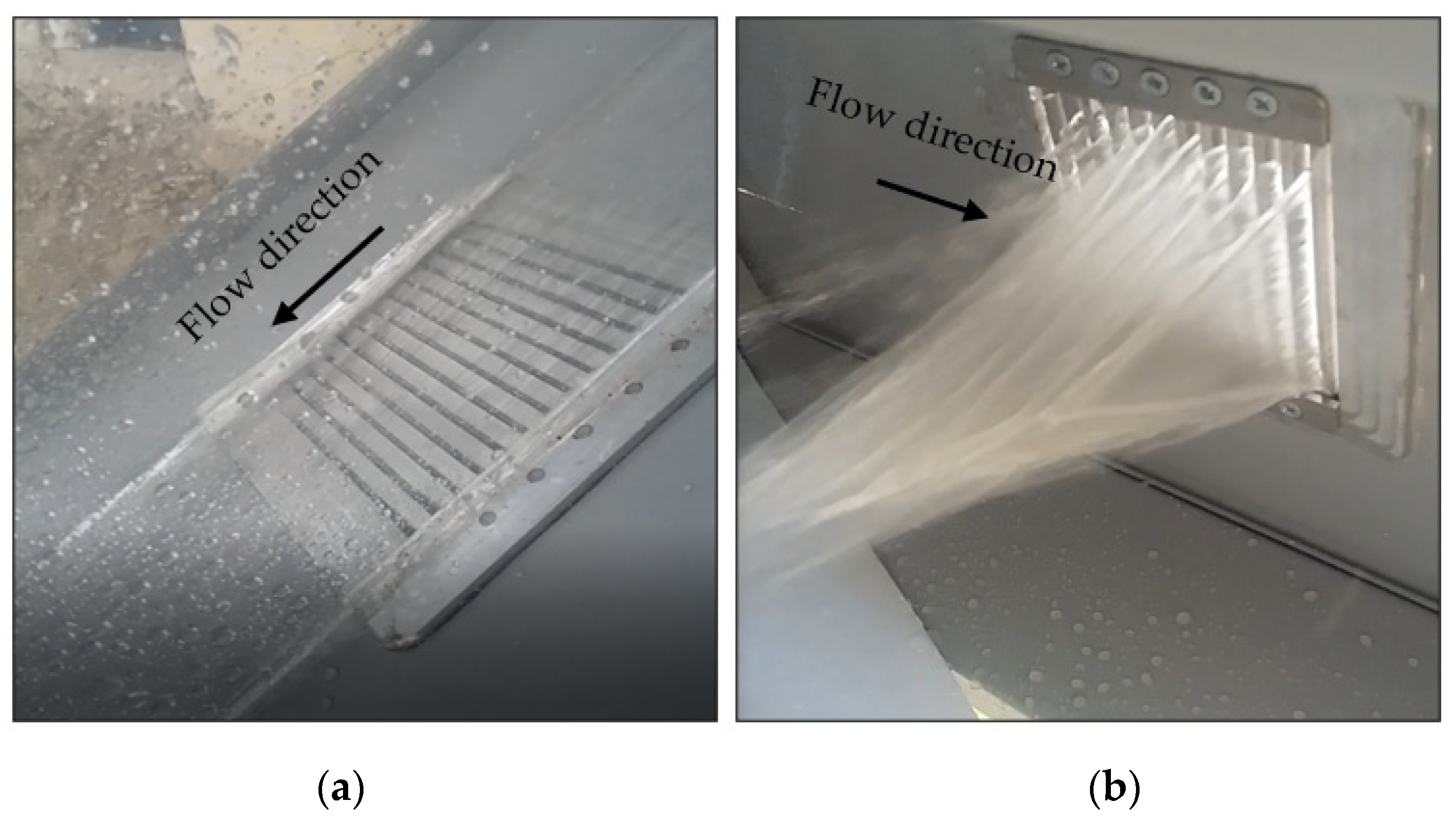
Figure 5 depicts one of the screens used in physical experimentation. Figure 5a shows the flow that passed over the Coanda-effect screen, and Figure 5b shows the flow of clean water captured through the screen’s openings. The volumetric method was used to measure the flow rate.
3.1.1. Clean Water
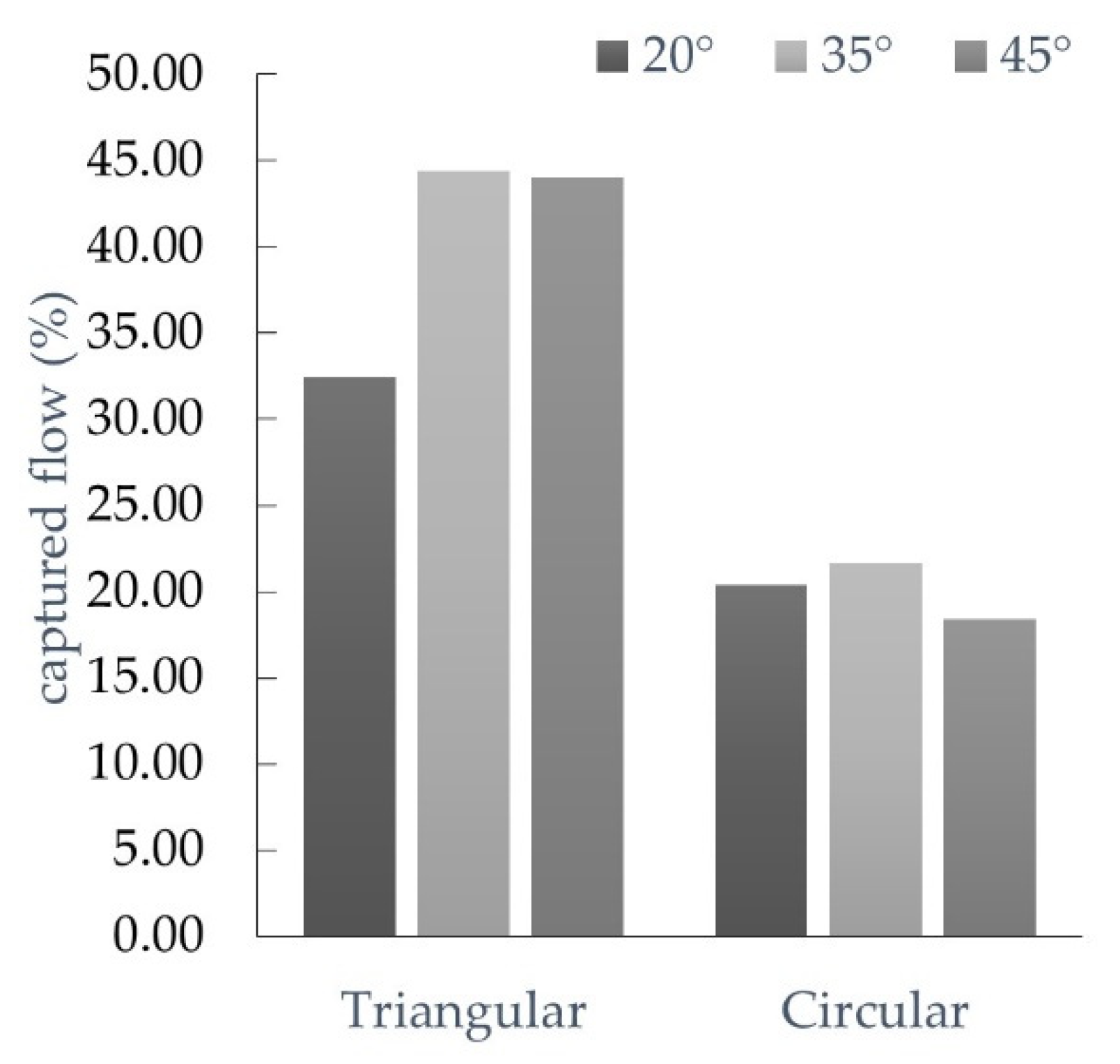
Figure 6 shows the flow of clean water captured by each type of screen for three angles of inclination (20°, 35°, and 45°). As can be seen, the grid with the highest efficiency in terms of the amount of flow captured was the triangular one, capturing 1.11 L/s for an inclination of 35°, which represents 44.4% of the total flow supplied for this study (2.5 L/s).
The higher capture efficiency of the triangular wire grid was attributed to the shear effect produced in the water due to its sharp edge and 5° inclination. Furthermore, the shear effect was zero in a circular wire, reducing the flow captured to 0.54 L/s for 35° of inclination.
3.1.2. Water with Sediment
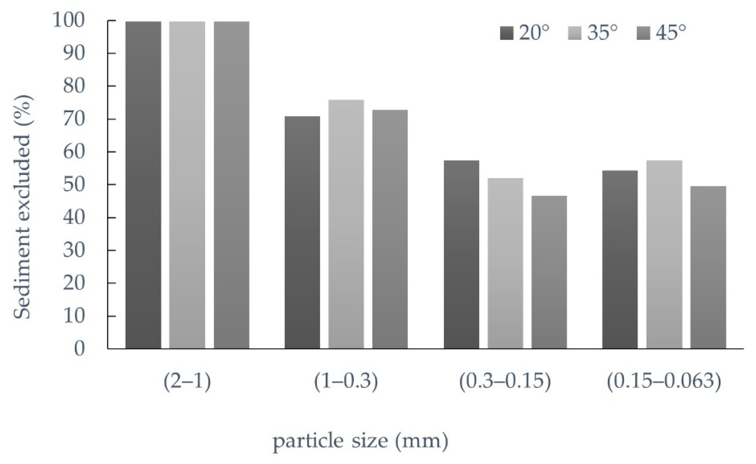
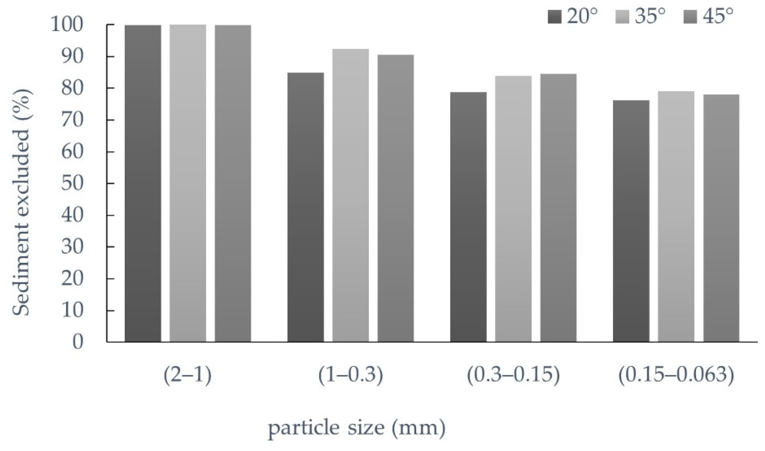
The percentage of sediment excluded for each particle size in the triangular and circular wire grids under the same flow, inclination, and sediment load conditions is shown in Figure 7 and Figure 8, respectively.
The percentage of sediment excluded was determinate by Equation (1).
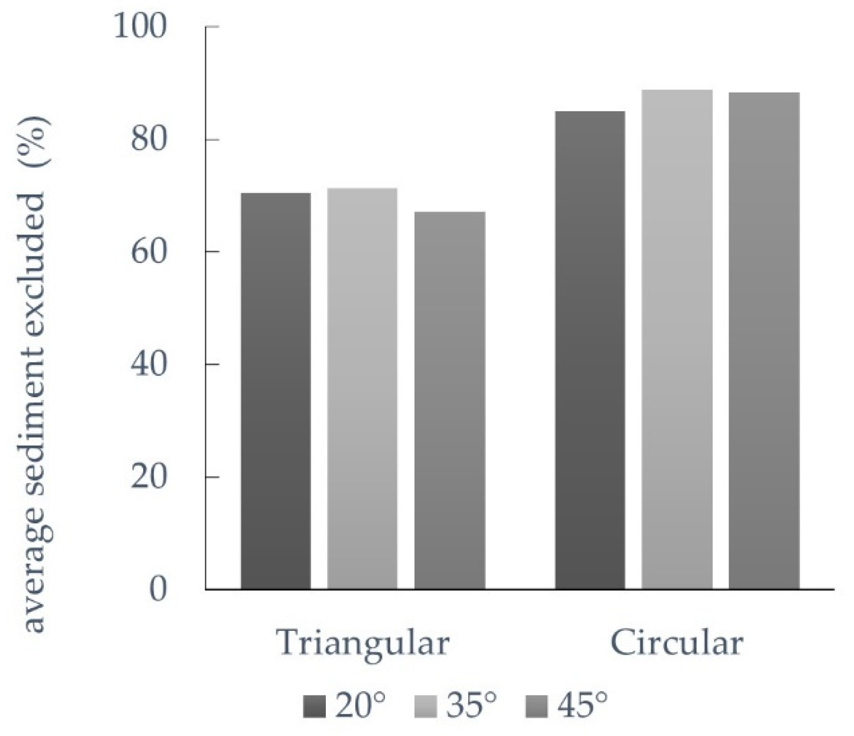
Figure 7 and Figure 8 show a higher exclusion percentage for all particle sizes in the circular wire screen. The smallest diameter particles in the range of 0.15–0.063 mm with 35° inclination were taken as reference. The circular wire screen prevented entry by up to 79.05% compared to the triangular wire grid, which prevented entry by up to 57.46%.
Figure 9 presents the average percentage of sediment excluded for the triangular- and circular- shaped wires. The circular wire screen is the most efficient in terms of the rate of sediment excluded, with 88.80%. However, the sediment exclusion percentage is not a value that completely represents the screen’s efficiency. In clean water tests, the triangular wire screen captured the most significant amount of water. In sediment tests, the circular screen excluded the more substantial amount of sediment. Hence, efficiency must be evaluated by considering the relationship between the captured flow and the excluded sediment.
3.1.3. Flow/Sediment Ratio Excluded
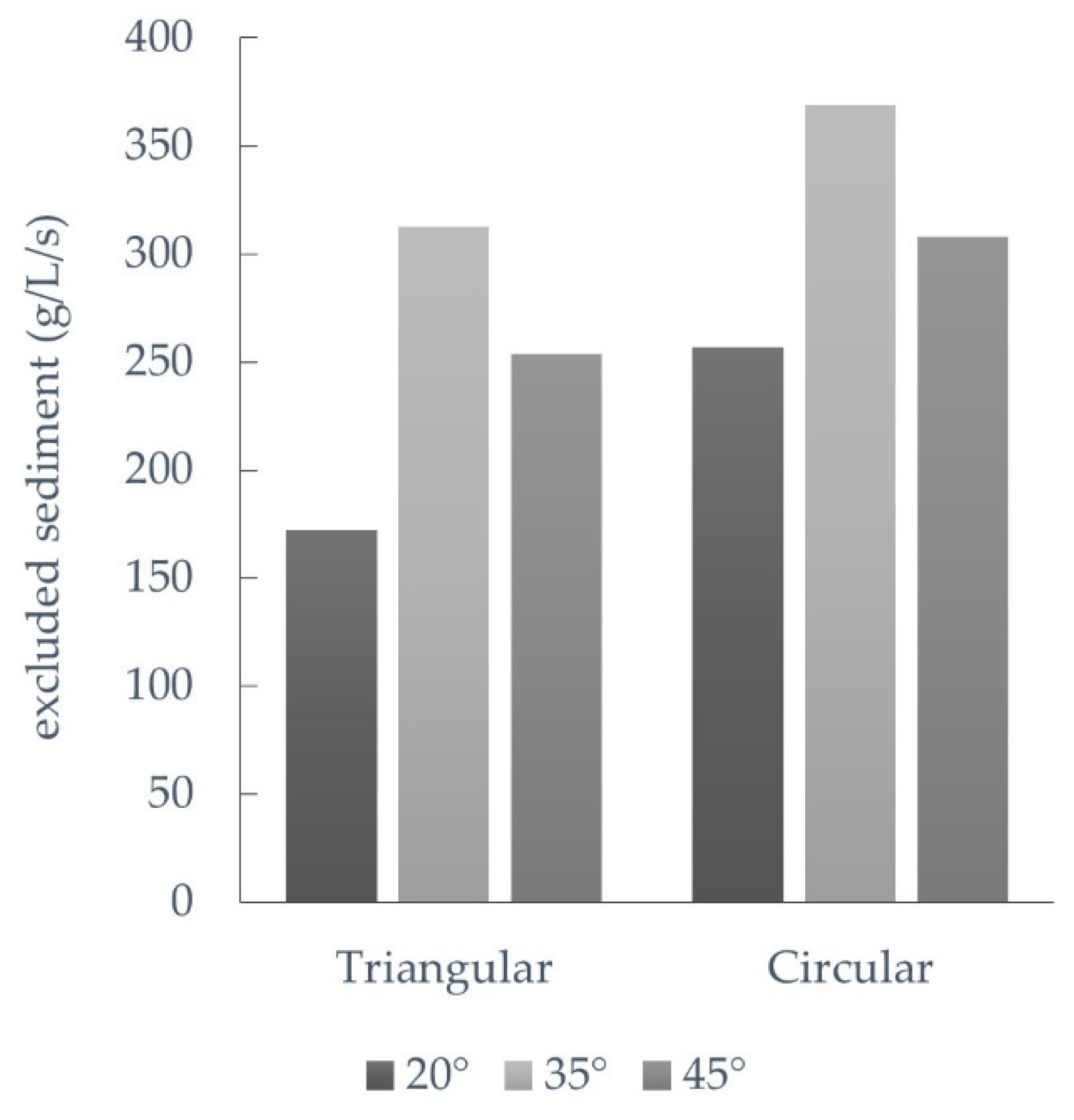
The relationship between the flow captured and the percentage of sediment excluded [18] can represent the efficiency of the screen in a more comprehensive form. Figure 10 depicts the specific (per L/s) amount of sediment excluded for both types of wires and tilt angles of 20°, 35°, and 45°.
Figure 10 shows that circular wire was more efficient at all tilt angles, and 35° was the optimum tilt angle.
3.2. Numerical Experimentation
3.2.1. Simulation Validation
The validation of the mathematical model was performed by comparison with selected results provided by Wahl [4]. Table 6 presents the analysis of meshing independence performed for the K–ω SST model.
Note that the percentage change of flow between the mesh of 0.05 mm and 0.04 mm was less than 2%. Likewise, the error between the laboratory and simulated flow was 2.67%. Therefore, it was considered that the mesh size and the established computational conditions were adequate to perform the CFD parametric study of the present work.
3.2.2. Comparison of the Flow Obtained with Experimental Data vs. Numerical Simulation
Table 7 presents a comparison between the results of four cases measured in the physical model and the flow rates obtained by CFD simulation. The maximum error was 4.31% for the simulation of the triangular wire screen at a 35°inclination, while the minimum error of 0.37% was presented in the circular wire screen at a 35° tilt.
The relative error was determinate by Equation (2).
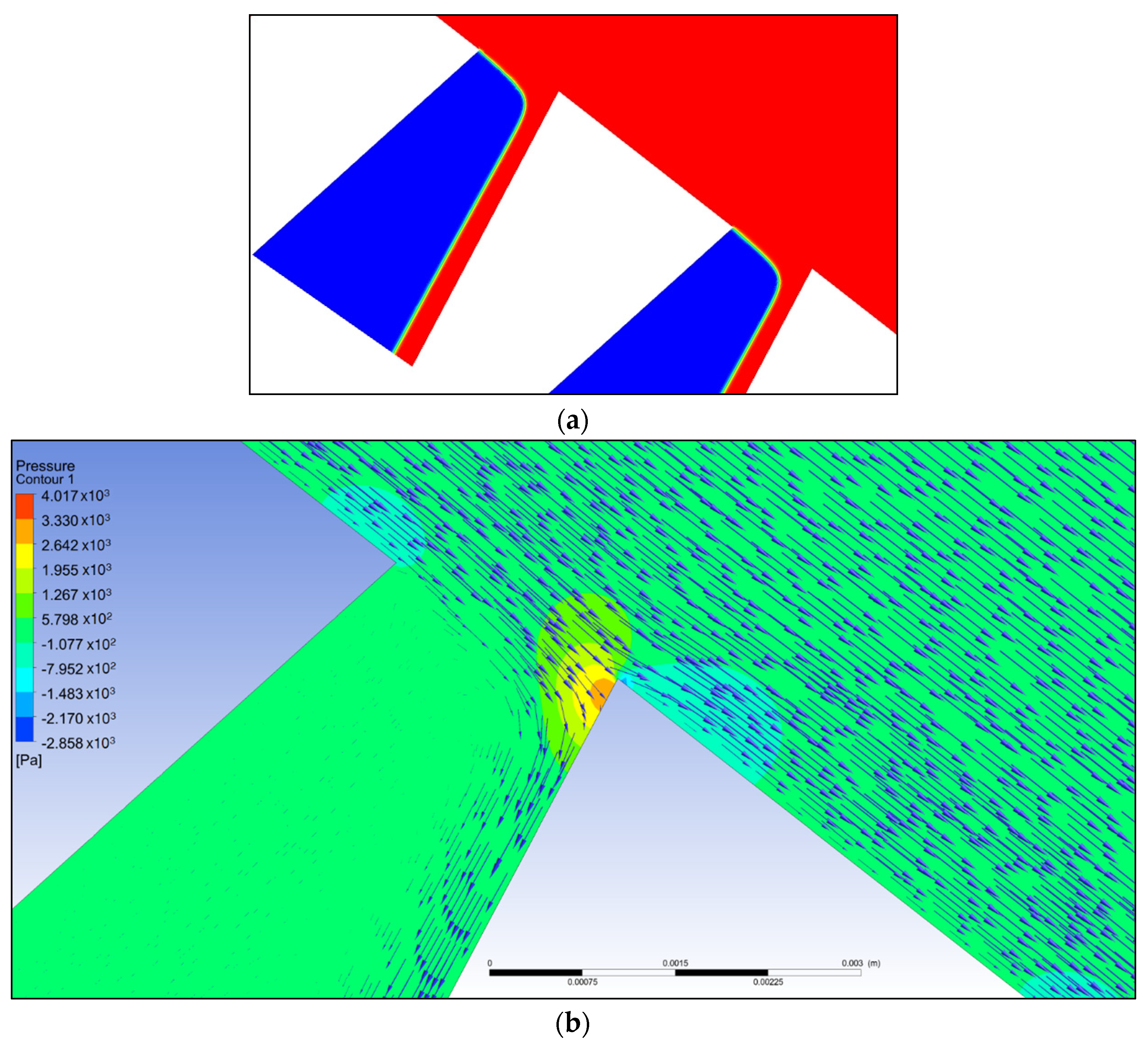
CFD Results from Triangular Wire Screen
The flow rates obtained by CFD had an error of less than 5% for the case of the triangular wire screen and an error of less than 1% for the case of the circular wire screen, so it was considered that the calibration of the computational model was adequate for the present study.
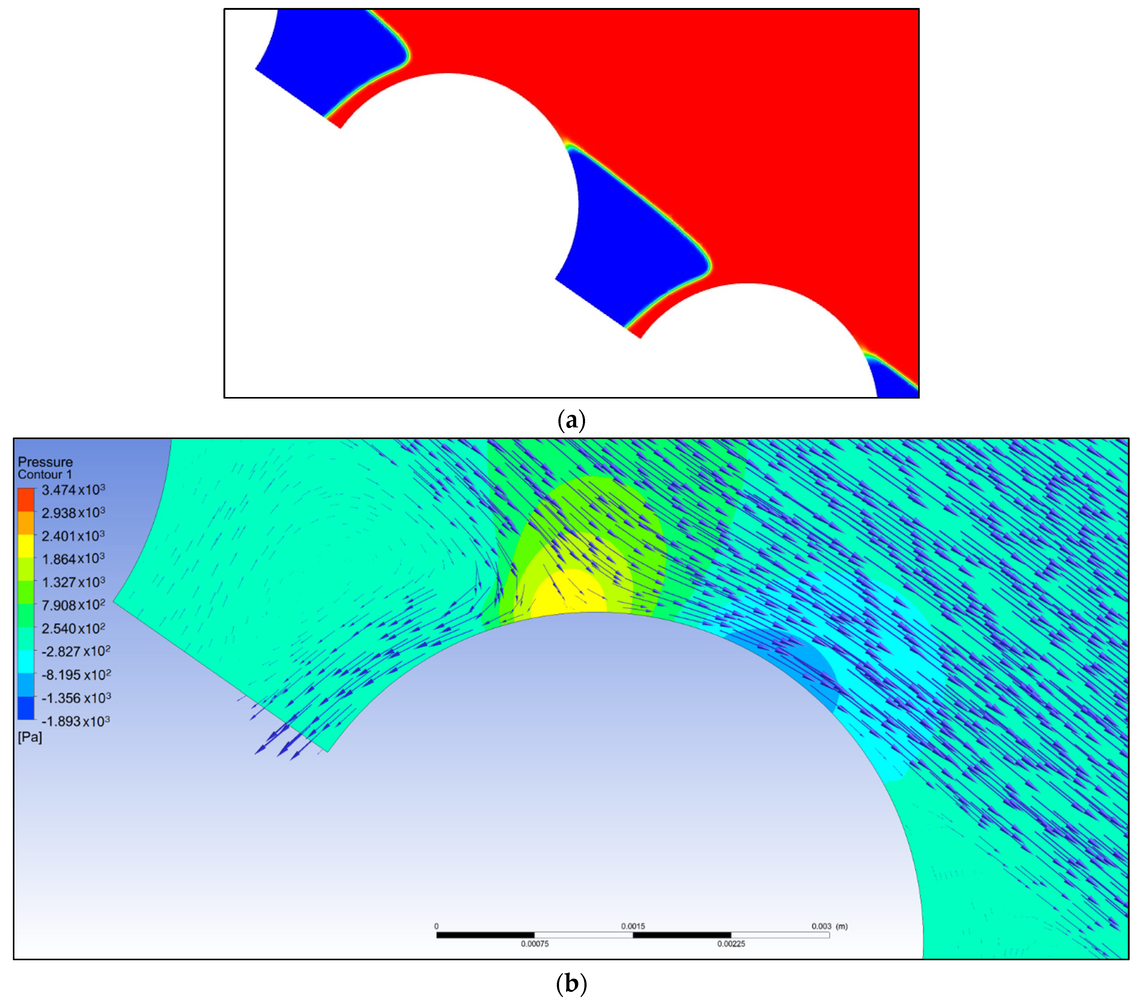
Figure 12b shows the trajectory of the velocity vectors and the pressure contours. The individual wires were tilted along their axes so that the leading edge of each wire projected into the flow, causing the screen to shear a thin layer of the flow from the bottom of the water column at each slot opening.
CFD Results from Circular Wire Screen
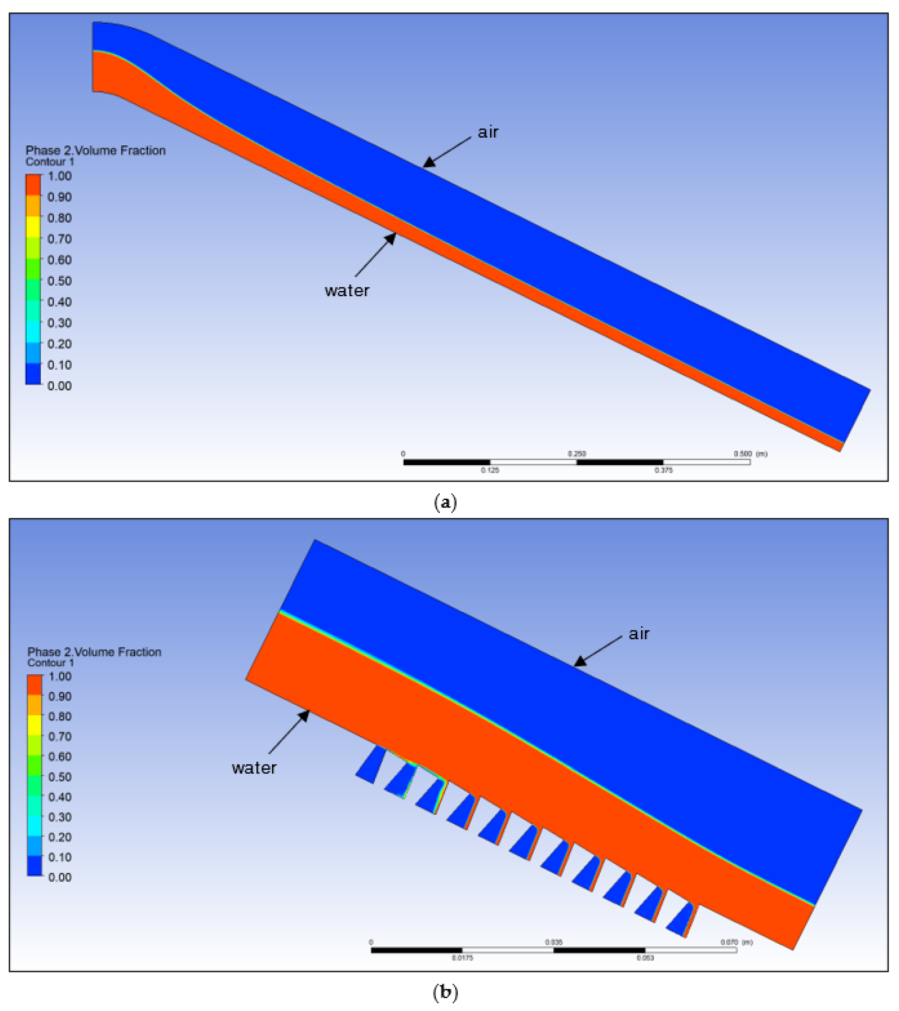
The simulated depth water profile close to the wall of the 5 mm circular wire screen at 35 degrees of inclination is shown in Figure 13a,b.
In the circular wire screen, the flow was diverted at the stagnation point that occurred after the sheet of water separated from the bar and jumped to the next one, colliding with the upper part.
The position of the stagnation point depends on the separation and the diameter of the wires. This position influences the flow captured by each slot.
3.2.3. 2D–CFD Parametric Study
A parametric CFD study was performed to determine the flow rate trend captured in each screen to evaluate the influence of variables such as shape, wire width, slot width, inclination, and position of the screens along the channel.
The slope and position of the screen along the channel modify the velocity and depth such that velocity increases and depth decreases downstream.
The efficiency of the screen was determined by the ratio between the captured flow (Δq) and the total flow supplied by the channel (q1). The influence of Froude and Reynolds number on Δq/q1 was explored.
The Froude number was calculated with the slope adjustment presented by Chow [27]
where
- F = Froude number,
- = mean velocity across the screen,
- = flow depth,
- θ = slope angle of the screen surface, measured from horizontal,
- g = acceleration due to gravity.
Reynolds numbers were computed using the depth-averaged mean velocity across the screen as the as the reference velocity and slot width as the reference longitude. The best correlations were obtained using the slot width to calculate the Reynolds number
where
- R = Reynolds number,
- V = mean velocity across the screen,
- s = open slot width between wires,
- ν = kinematic viscosity.
Triangular Wire Screen Performance
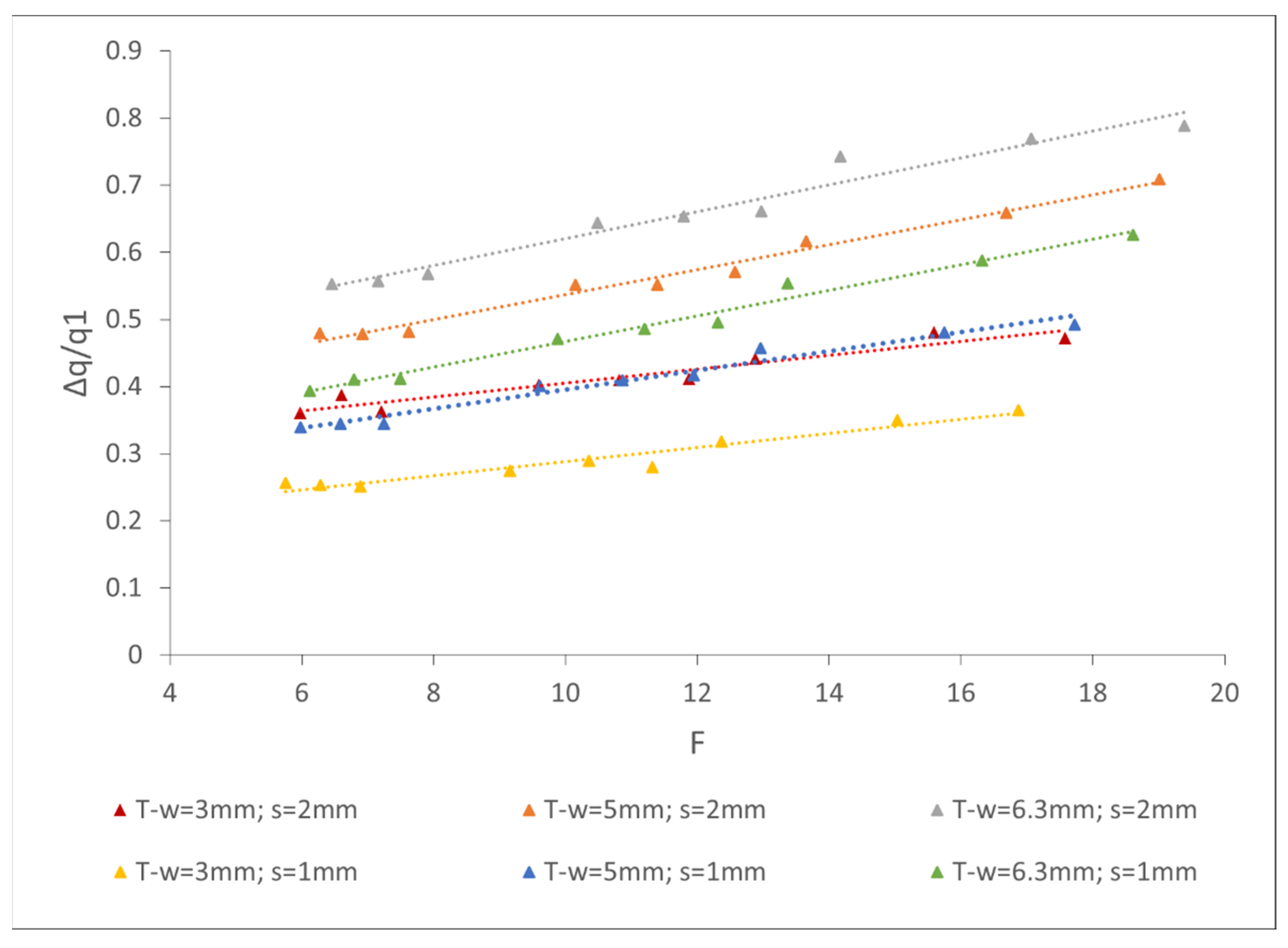
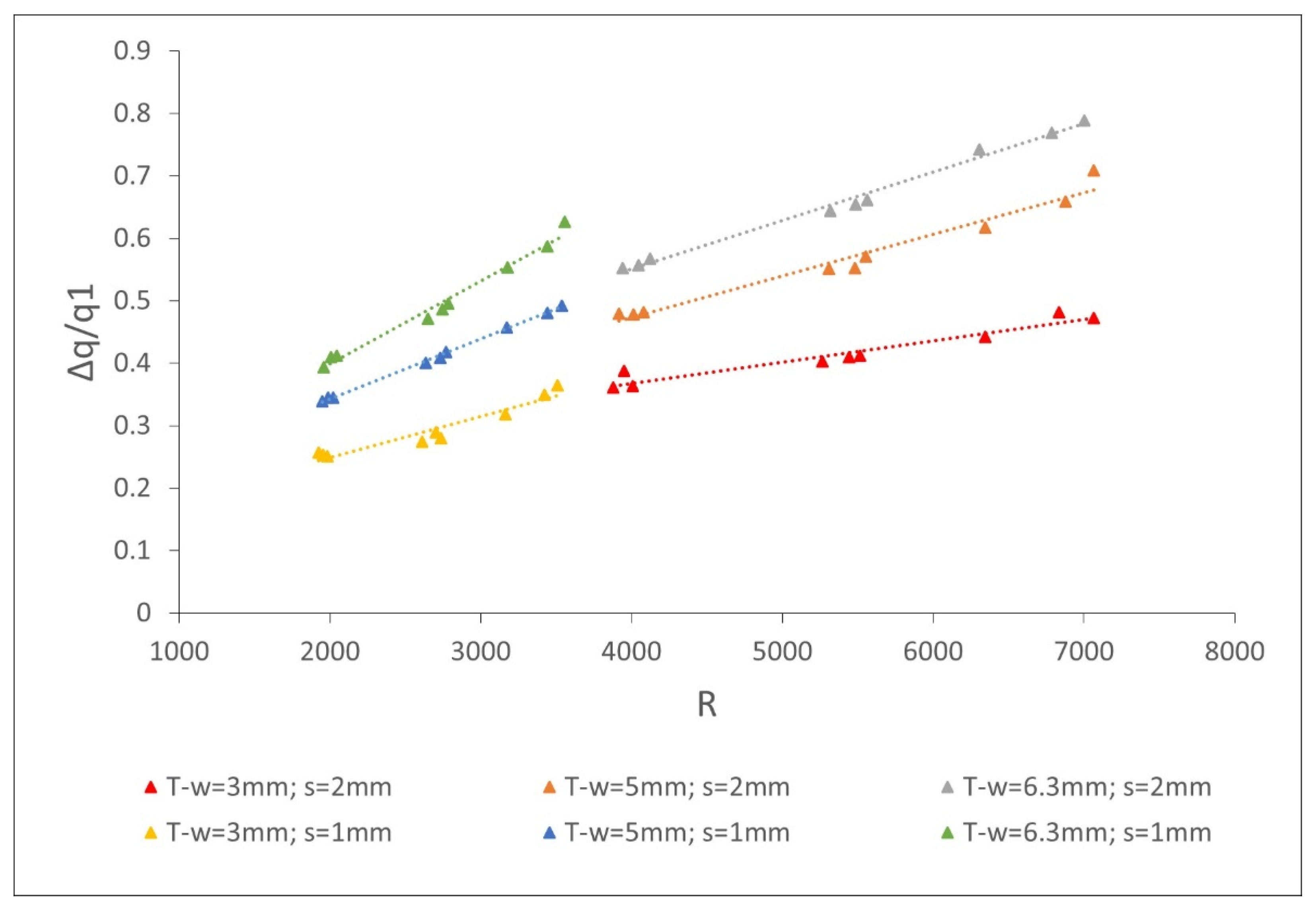
Figure 14 and Figure 15 depict the relations between Δq/q1 and Froude and Reynolds numbers, respectively. The charts show only data from the triangular wire screen. A nearly linear relationship with each parameter was evidenced, as flow captured by the triangular wire screen increased as the values of F and R increased. The highest values were higher channel slopes and high flow velocities (i.e., screens installed in bottom test positions).
A nearly linear relationship was also observed between the flow rate captured and the width of the wire, maintaining the trend concerning the numbers of F and R.
The cases with Reynolds number greater than 4000 corresponded to the wires with the greatest separation (2 mm). For this reason Δq/q1 was greater than the group of cases with R < 4000.
If the flow velocity across the screen face, V, was presumed to remain constant as the flow turns. Then, the unit discharge through the screen at each wire was simply [4]:
where = offset height created by tilted wire.
By increasing the width wire and slot wire, also increased. For this reason, the screen that captured the highest flow was the T-w = 6.3 mm; s = 2 mm.
For circular wire screens, the numerical experimentation was performed under the same geometric and flow conditions of the triangular wire screen. The wire diameters used were equivalent to the wire widths of the triangular wires (3 mm, 5 mm, and 6.3 mm). In addition, commercially available higher wire diameters were studied (10 mm, 16 mm and 20 mm).
Circular Wire Screen Performance
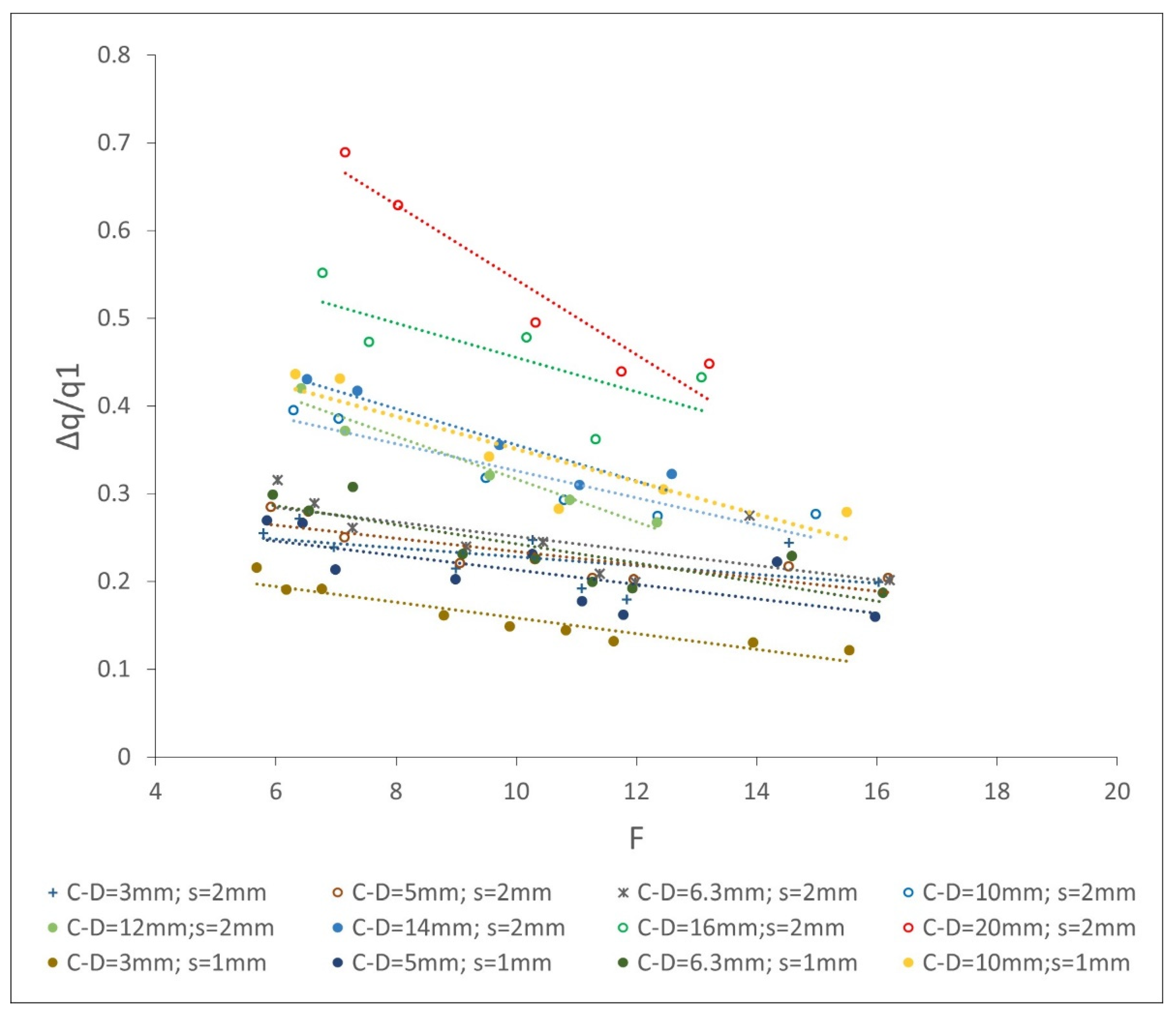
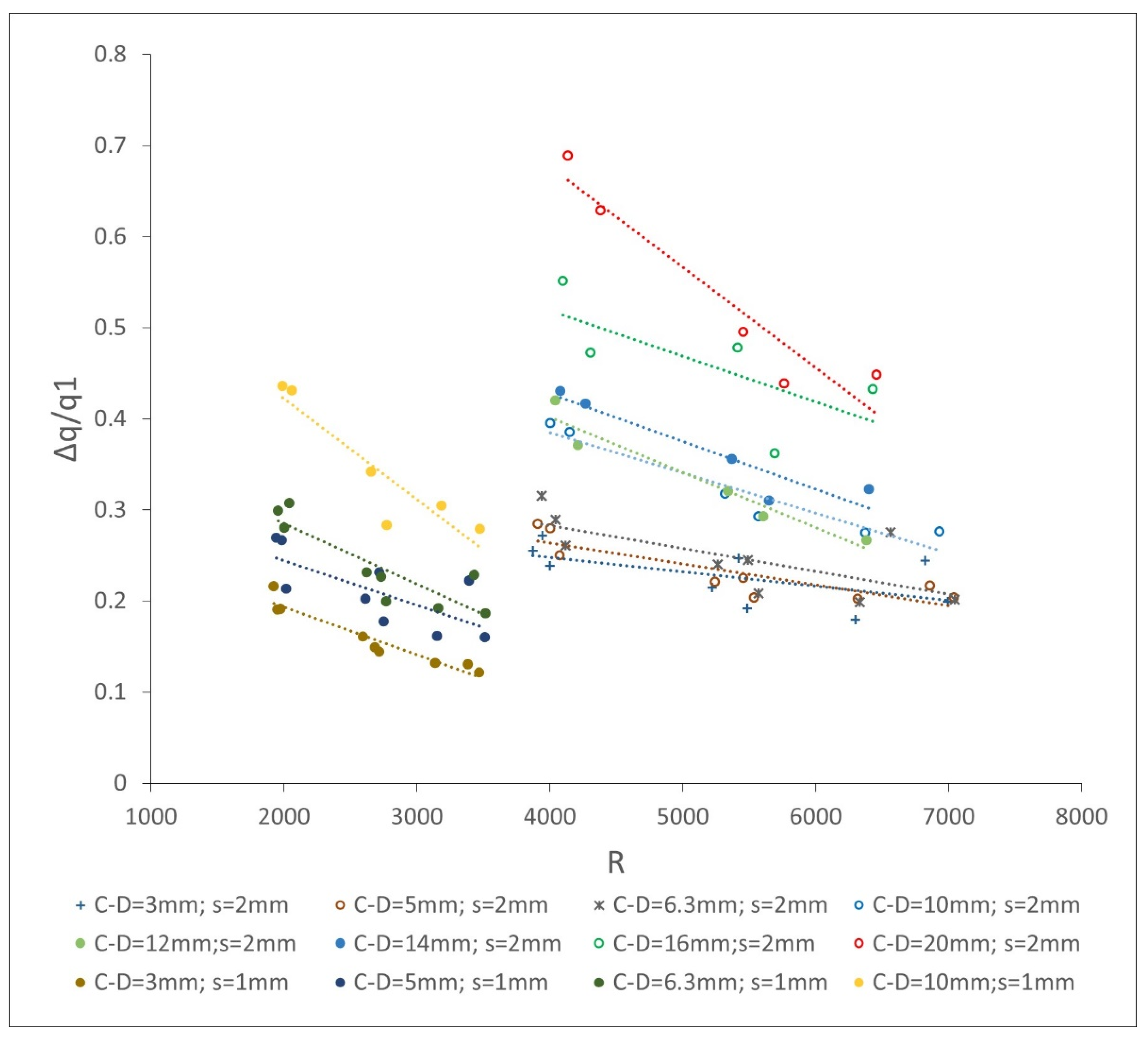
Figure 16 and Figure 17 depict relations between Δq/q1 and F, R, respectively, from circular wire screen data. In most cases, triangular and circular bars behaved oppositely, and an inverse nearly linear relationship between the captured flow and F, R was evidenced. The flow captured by the circular wire screen decreased as the values of F and R increased. Higher values occurred for lower channel slopes and low flow velocities (i.e., screens installed in top test positions).
Like a triangular wire screen, a circular wire screen has a nearly linear relationship between the diameter of the wire and the flow rate captured, maintaining the trend concerning F and R. Larger wire diameters increase the contact surface and the length of the screen, which increases the collection capacity. Numerical experimentation generated results consisting of bars up to 20 mm in diameter with a wire slot of 2 mm. The simulation of bars with a slot of 1 mm was restricted to 10 mm in diameter due to irregularities such as vortices and reversed flow in the wires with diameter of 16 mm and higher. For this reason, these results were not considered in Figure 17.
With 70% of the flow captured, the 20 mm diameter wire screen with a 2 mm slot located in the top position of the channel, with a 20-degree inclination, presented the best performance.
The 3 mm diameter wire screen with a 1 mm slot situated in the bottom position of the channel, with a 45-degree slope, captured 12% of the flow and presented the lowest efficiency.
4. Conclusions
Physical experimentation showed that the triangular wire screen was more efficient regarding the flow captured. In contrast, the circular wire screen was more efficient in sediment removal.
The 2D numerical experimentation allowed us to obtain qualitative and quantitative results highly consistent with the laboratory results. The accuracy of Ansys Fluent was evaluated with clean water. The mesh independence test presented satisfactory results with elements of the size of 0.04 mm in the zone of the screen wires.
Numerical experiments performed with different positions and inclinations showed that screens with triangular and circular bars had opposite behaviors. The screens with triangular bars were more efficient in terms of flow captured as R and F increased, while those with circular bars were more efficient as R and F decreased.
In general, using equal sizes of bars and separations (same R and F), screens with triangular bars were more efficient than those with circular bars. Numerical experiments with circular bars screens showed that increasing the size of the bars maintaining the separation increased the efficiency of flow captured to a similar level than triangular bar screens. It is important to remark that screens with circular bars are cheaper, easier to build, and may be a good choice for sediment removal. In the case that a higher flow efficiency is desirable, using circular bars with bigger diameters would be preferable.
Author Contributions
E.C.-C.: Investigation, Writing—Original Draft; Writing—Review & Editing; Visualization, Project administration, Funding acquisition/P.O.: Conceptualization, Writing—Review & Editing, Supervision, Visualization/L.N.: Conceptualization, Writing—Review & Editing, Supervision, Visualization. All authors have read and agreed to the published version of the manuscript.
Funding
This research was financially supported by Universidad Técnica Particular de Loja, Ecuador.
Conflicts of Interest
The authors declare no conflict of interest.
References
- Brunella, S.; Hager, W.H.; Minor, H.-E. Hydraulics of Bottom Rack Intake. J. Hydraul. Eng. 2003, 129, 2–10. [Google Scholar] [CrossRef]
- Righetti, M.; Lanzoni, S. Experimental Study of the Flow Field over Bottom Intake Racks. J. Hydraul. Eng. 2008, 134, 15–22. [Google Scholar] [CrossRef] [Green Version]
- Carrillo, J.M.; García, J.T.; Castillo, L.G. Experimental and Numerical Modelling of Bottom Intake Racks with Circular Bars. Water 2018, 10, 605. [Google Scholar] [CrossRef] [Green Version]
- Wahl, T.L.; Shupe, C.C.; Dzafo, H.; Dzaferovic, E. Surface Tension Effects on Discharge Capacity of Coanda-Effect Screens. J. Hydraul. Eng. 2021, 147, 04021026. [Google Scholar] [CrossRef]
- Finch, H.E.; Strong, J.J. Self-cleaning screen. U.S. Patent No. 4415462A, 15 November 1983. [Google Scholar]
- Strong, J.J.; Ott, R.F. Intake screens for small hydro plants. Hydro Rev. 1988, 7, 66–69. [Google Scholar]
- Ansys Inc. “ANSYS FLUENT Theory Guide,” ANSYS Inc., USA, vol. Release 20, no. R1, p. 814, 2020, [Online]. Available online: http://www.afs.enea.it/project/neptunius/docs/fluent/html/th/main_pre.htm (accessed on 14 December 2020).
- Bouvard, M. Discharge Passing through a Bottom Grid. Houille Blanche 1953, 2, 290–291. [Google Scholar] [CrossRef] [Green Version]
- Kuntzmann, M.; Bouvard, J. Theoretical Study of Bottom Type Water /make Grids. Houille Blanche 1954, 3, 569–574. [Google Scholar] [CrossRef] [Green Version]
- Mostkow, M.A. A Theoretical Study of Bottom Type Water intake. Houille Blanche 1957, 4, 570–580. [Google Scholar] [CrossRef] [Green Version]
- Jain, A.K.; Asawa, J.K.; Mehrotra, G.L. Bottom Racks-An Experimental Study. J. Irrig. Power 1975, 3, 219–222. [Google Scholar]
- Ranga Raju, K.G.; Asawa, G.L.; Seetharamaiah, R. Analysis of Flow through Bottom Racks in Open Channels. In Proceedings of the 61th Australasian Hydraulics and Fluid Mechanics Conference, Adelaide, Australia, 5–9 December 1977. [Google Scholar]
- Subramanya, D.; Sengupta, K. Flow through Bottom Racks. Indian J. Technol. 1981, 19, 64–67. [Google Scholar]
- Wahl, T.L.; Einhellig, R.F. Laboratory Testing and Numerical Modeling of Coanda-Effect Screens. In Proceedings of the Joint Conference on Water Resource Engineering and Water Resources Planning and Management, Minneapolis, MN, USA, 30 July–2 August 2000. [Google Scholar]
- Wahl, T.L. Hydraulic Performance of Coanda-Effect Screens. J. Hydraul. Eng. 2001, 127, 480–488. [Google Scholar] [CrossRef]
- Ojha, C.S.; Shankar, V.; Chauhan, N.S. Analysis of flow over horizontal transverse bottom racks. ISH J. Hydraul. Eng. 2007, 13, 41–52. [Google Scholar] [CrossRef]
- Esmond, S. Effectiveness of Coanda Screens for Removal of Sediment, Nutrients, and Metals from Urban Runoff. In Proceedings of the 43rd International Erosion Control Association Annual Conference, Las Vegas, NV, USA, 26–29 February 2012. [Google Scholar]
- May, D. Sediment Exclusion from Water Systems Using a Coanda Effect Device. Int. J. Hydraul. Eng. 2015, 4, 23–30. [Google Scholar] [CrossRef]
- Wahl, T.L. New Testing of Coanda-Effect Screen Capacities. In Proceedings of the HydroVision International, Denver, CO, USA, 23–26 July 2013. [Google Scholar]
- Yun, S.-M.; Kim, Y.-S.; Shin, H.-J.; Ko, S.-C. A Numerical Study for Optimum Design of Dust Separator Screen Based on Coanda Effect. Korean Soc. Manuf. Process. Eng. 2018, 17, 177–185. [Google Scholar] [CrossRef]
- Chanson, C.; Gualtieri, H. Similitude and scale effects of air entrainment in hydraulic jumps. J. Hydraul. Res. 2008, 46, 35–44. [Google Scholar] [CrossRef] [Green Version]
- Bombardelli, F.A. Computational multi-phase fluid dynamics to address flows past hydraulic structures. In Proceedings of the 4th IAHR International Symposium on Hydraulic Structures, Brisbane, Australia, 25–27 June 2012. [Google Scholar]
- Blocken, C.; Gualtieri, B. Ten iterative steps for model development and evaluation applied to Computational Fluid Dynamics for Environmental Fluid Mechanics. J. Environ. Model. Softw. 2012, 33, 1–22. [Google Scholar] [CrossRef]
- Ferziger, M.P.J.H.; Peric, M.; Street, R.L. Computational Methods for Fluid Dynamics; Springer: Berlin, Germany, 2002. [Google Scholar]
- Menter, F.R. Two-equation eddy-viscosity turbulence models for engineering applications. AIAA J. 1994, 32, 1598–1605. [Google Scholar] [CrossRef] [Green Version]
- Ghobadian, S.A.V.A. A General Purpose Implicit Coupled Algorithm for the Solution of Eulerian Multiphase Transport Equation. In Proceedings of the International Conference on Multiphase Flow, Lisbon, Portugal, 17–19 June 2007. [Google Scholar]
- Chow, V.T. Open-Channel Hydraulics; McGraw-Hill: New York, NY, USA, 1959. [Google Scholar]
Figure 1.
Detail of screen geometry and key variables. (Adapted from [4]).
Figure 1.
Detail of screen geometry and key variables. (Adapted from [4]).

Figure 2.
(a) Variable-slope screen testing flume; (b) screen installed in the test flume; (c) test screen triangular wire (d) test screen circular wire.
Figure 2.
(a) Variable-slope screen testing flume; (b) screen installed in the test flume; (c) test screen triangular wire (d) test screen circular wire.

Figure 3.
Geometry 2D of computational domain: (a) flume; (b,c) triangular wire screen; (d,e) circular wire screen.
Figure 3.
Geometry 2D of computational domain: (a) flume; (b,c) triangular wire screen; (d,e) circular wire screen.

Figure 4.
2D tetrahedrical mesh in the computational domain: (a) triangular wire screen mesh; (b) circular wire screen mesh.
Figure 4.
2D tetrahedrical mesh in the computational domain: (a) triangular wire screen mesh; (b) circular wire screen mesh.

Figure 5.
(a) Flow over Coanda screen; (b) diverted flow.

Figure 6.
Graph of the clean water flow captured by a triangular and circular wire screen.

Figure 7.
Graph of percentage of the sediment excluded by a triangular wire screen.

Figure 8.
Graph of the percentage of sediment excluded by a circular wire screen.

Figure 9.
Graph of the average percentage of sediment excluded.

Figure 10.
Graph of sediment excluded by each type of screen.

Figure 11.
Two-phase contour volume fraction: (a) channel domain; (b) A5 test screen; (c) pressure contours; (d) velocity contours.
Figure 11.
Two-phase contour volume fraction: (a) channel domain; (b) A5 test screen; (c) pressure contours; (d) velocity contours.


Figure 12.
CFD simulation results of the triangular wire screen: (a) two-phase contour volume fraction; (b) vectors velocity and pressure contours.
Figure 12.
CFD simulation results of the triangular wire screen: (a) two-phase contour volume fraction; (b) vectors velocity and pressure contours.

Figure 13.
CFD simulation results of circular wire screen; (a) two-phase contour volume fraction; (b) vectors velocity and pressure contours.
Figure 13.
CFD simulation results of circular wire screen; (a) two-phase contour volume fraction; (b) vectors velocity and pressure contours.

Figure 14.
Relations for triangular wire screen between Δq/q1 and Froude number.

Figure 15.
Relations for triangular wire screen between Δq/q1 and Reynolds number.

Figure 16.
Relations for circular wire screen between Δq/q1 and Froude number.

Figure 17.
Relations for circular wire screen between Δq/q1 and Reynolds number.


Table 1.
Geometric Features of the Test Screens Used.
| Screen | 1 | 2 |
|---|---|---|
| Section | Triangular | Circular |
| Test width (cm) | 9.3 | 9.3 |
| Wire tilt angle (degrees) | 5 | - |
| Average slot width, s (mm) | 2 | 2 |
| Average wire thickness, w (mm) | 5 | 5 |
| Number of wires | 12 | 12 |
| Positions tested | bottom | bottom |
Table 2.
Boundary Conditions Applied.
| Model Boundary | Boundary Conditions |
|---|---|
| Walls | No-slip |
| Inlet channel | mass flow inlet |
| Inlet screen | velocity-inlet |
| Outlet | pressure-outlet |
| Atmosphere | pressure-outlet |
Table 3.
Properties of the Continuous Phases.
| Property | Phase 1 | Phase 2 |
|---|---|---|
| Material | air | water |
| Density (kg/m3) | 1.225 | 998.2 |
| Dynamic viscosity (kg/ms) | 1.7894 × 10⁻⁵ | 0.001003 |
| Surface tension coefficient (N/m) | 0.072 | |
Table 4.
Numerical Schemes and Solution Methods [7].
Table 4.
Numerical Schemes and Solution Methods [7].
| Variable | Adjustment |
|---|---|
| Turbulence model | k–ω SST |
| Pressure velocity coupling | Coupled |
| Gradient | Least Squares Cell-Based |
| Pressure | Body Force Weighted |
| Momentum | Second-order upwind |
| Volume fraction | Compressive |
| Turbulence Kinetic Energy | Second-order upwind |
| Turbulence Dissipation rate | Second-order upwind |
| Initialization | Standard |
Table 5.
Validation Screen Properties.
| Screen | A5 |
|---|---|
| Relief angle (λ°) | 10 |
| Test width (cm) | 5.08 |
| Wire Width, w (mm) | 4.7167 |
| Slot Width, s (mm) | 1.985 |
| Wire Tilt, φ | 5.25 |
| Waste Slots | 5 |
| Test Slots | 6 |
| Screen Incline θ° | 26.3 |
| Test Location | bottom |
| Distance down straight chute to first slot (mm) | 1094.978 |
| Conditions at the crest (critical depth) (mm) | 58.80 |
| Flow in (L/s) | 2.2684 |
| Screened flow (L/s) | 0.487 |
Table 6.
Mesh Convergence for the A5 Test Screen.
| Element Mesh Size (mm) | Number of Nodes | Laboratory Flow (L/s) | CFD Flow (L/s) | Relative Error (%) | Relative Error Laboratory Flow vs. CFD Model (%) |
|---|---|---|---|---|---|
| 0.2 | 39,510 | 0.487 | 0.396 | -- | 18.69 |
| 0.1 | 155,721 | 0.487 | 0.440 | 11.11 | 9.65 |
| 0.05 | 501,376 | 0.487 | 0.466 | 5.91 | 4.31 |
| 0.04 | 671,511 | 0.487 | 0.474 | 1.72 | 2.67 |
Table 7.
Comparison of the Flow Obtained with Experimental Data vs. Numerical Simulation.
| Screen | Screen Incline (°) | Laboratory Flow (L/s) | CFD Flow k–ω SST Model (L/s) | Relative Error Laboratory Flow vs. k–ω SST Model (%) |
|---|---|---|---|---|
| Triangular wire | 35 | 1.11 | 1.16 | 4.31 |
| 45 | 1.1 | 1.14 | 3.51 | |
| Circular wire | 20 | 0.51 | 0.505 | 0.99 |
| 35 | 0.54 | 0.542 | 0.37 |
Publisher’s Note: MDPI stays neutral with regard to jurisdictional claims in published maps and institutional affiliations. |
© 2022 by the authors. Licensee MDPI, Basel, Switzerland. This article is an open access article distributed under the terms and conditions of the Creative Commons Attribution (CC BY) license (https://creativecommons.org/licenses/by/4.0/).
Share and Cite
MDPI and ACS Style
Carrión-Coronel, E.; Ortiz, P.; Nanía, L. Physical Experimentation and 2D-CFD Parametric Study of Flow through Transverse Bottom Racks. Water 2022, 14, 955. https://doi.org/10.3390/w14060955
AMA Style
Carrión-Coronel E, Ortiz P, Nanía L. Physical Experimentation and 2D-CFD Parametric Study of Flow through Transverse Bottom Racks. Water. 2022; 14(6):955. https://doi.org/10.3390/w14060955
Chicago/Turabian StyleCarrión-Coronel, Eduardo, Pablo Ortiz, and Leonardo Nanía. 2022. "Physical Experimentation and 2D-CFD Parametric Study of Flow through Transverse Bottom Racks" Water 14, no. 6: 955. https://doi.org/10.3390/w14060955
Note that from the first issue of 2016, this journal uses article numbers instead of page numbers. See further details here.