Modeling Cyanobacteria Vertical Migration

Abstract

Cyanobacteria often cause harmful algal blooms and release toxic substances that can harm humans and animals. Accurately modeling these phytoplankton is a step towards predicting, preventing, and controlling such blooms. Certain cyanobacteria species are known to migrate vertically in the water column on a daily cycle. Capturing this behavior is one aspect of modeling their dynamics. Previous studies on modeling cyanobacterial vertical migration are reviewed and summarized. Several models of cyanobacteria vertical movement are tested using data from field studies. These models are applied using both continuum and particle-tracking frameworks. Models range in complexity from simple functions of time to more complicated calculations of cyanobacteria buoyancy. Simple models were often able to predict cyanobacteria migration at low values of vertical diffusion in both types of modeling frameworks. More complicated models of buoyancy change performed better in the particle-tracking framework than in the continuum framework. Analysis of the models developed and tested provides information on the applicability of these models in more complex hydrodynamic and water quality models.

1. Introduction

1.1. Background

Cyanobacteria are often responsible for harmful algae blooms (HABs), which occur when these phytoplankton grow excessively in a waterbody. Several genera of cyanobacteria, including Microcystis, Oscillatoria, Anabaena, and Aphanizomenon, produce toxic substances called cyanotoxins, which can cause serious health problems in humans and other mammals [1,2]. Some are able to move vertically in the water column by their own motility, independent of water velocity [3]. The vertical migration of species such as Microcystis aeruginosa, Oscillatoria agardhii, and Anabaena flos-aqua can lead to HABs when colonies accumulate on a water surface and experience increased growth, causing degradation of water quality and environmental health [4].

Vertical migration is thought to be beneficial to cyanobacteria because it allows them to travel between the surface layers of a waterbody, where light is abundant, and lower, more nutrient-rich layers [5]. Some studies suggest that cyanobacteria are able to move past the thermocline of a lake to take advantage of nutrients in the hypolimnion [6], while others found insufficient evidence that this occurs in natural systems [7]. Nevertheless, this movement is achieved through a process called buoyancy regulation. Cells regulate their buoyancy either through carbohydrate ballast or gas vesicles [8]. Carbohydrates are accumulated when cells photosynthesize, and this ballast causes a decrease in buoyancy and subsequent sinking. Once cells have stopped photosynthesizing, the carbohydrates are consumed, the ballast depleted, and cells rise again [9]. Chemicals accumulated during photosynthesis also cause gas vesicles contained in cells to collapse through turgor pressure, which decreases buoyancy. Synthesis of new gas vesicles leads to an increase in buoyancy [10].

Based on these mechanisms, buoyancy regulation and vertical migration are affected by external factors such as light and nutrients. Laboratory experiments on O. agardhii showed that carbohydrate ballast (and, therefore, density) increased with increasing irradiance, then leveled off and eventually decreased after light ceased [8]. Ibelings et al. [11] observed that Microcystis colonies in two lakes in the Netherlands decreased in buoyancy during the day and increased at night, following a diurnal light cycle. Similar results were found by Cui et al. [12] in the Three Gorges Reservoir. Visser et al. [13] found a positive relationship between carbohydrate content and density of Microcystis cells in laboratory experiments. They also found that the rate of cell density change increased with increasing photon irradiance up to a point, then decreased as photon irradiance continued to increase. Their experiments showed that after light ceased, the rate of density decrease was greater when initial cell density was greater. Wallace and Hamilton [14] performed similar experiments on M. aeruginosa in the laboratory and confirmed the positive relationship between cell density and carbohydrate content found by Visser et al. [13]. They also proposed the existence of a “response time” that occurs when cells are first exposed to light. Until the end of the response time, cell density does not increase constantly with light. Laboratory experiments on M. aeruginosa suggest that buoyancy regulation is dependent on the light and nutrient history experienced by cells, as well as persisting light and nutrient conditions [5].

Exogenous factors besides light and nutrients have been found to affect cyanobacteria distributions. In Lake Taihu in China, surface blooms of M. aeruginosa did not form when wind speed and surface wave height exceeded critical values of 3.1 m/s and 0.062 m, respectively [15]. Microcystis colonies in the Three Gorges Reservoir were observed to migrate to greater depths in open water while those in a protected enclosure stayed closer to the surface [12]. Zhao et al. [16] found that Microcystis spp. (mainly M. aeruginosa) in a laboratory experiment could maintain buoyancy up to a critical value of turbulent kinetic energy, and that this value increased with colony size. They hypothesized that larger colonies were better able to overcome turbulent entrainment due to their greater diameter, which increases drag force. Similar results were found by Zhu et al. [17] in Lake Taihu. In response to the tendency of cyanobacteria species to thrive in stratified systems, artificial mixing techniques are often used to control and prevent blooms. These include aeration and pumping water between the hypolimnion and epilimnion to decrease stratification and increase turbulence [3]. This disrupts the stability that allows the cyanobacteria to stay at the water surface and can displace them to deeper parts of the water column where growing conditions are less favorable.

Due to the serious health effects caused by HABs and their increasing frequency of occurrence in waterbodies [18], it is desirable to be able to model the organisms responsible for them accurately. The purpose of this study was to develop models of cyanobacteria that are able to accurately predict their vertical migration. We first reviewed existing models of cyanobacteria vertical migration and then selected several models that were tested and compared to field data. These models ranged in complexity, with the simplest based on predefined velocity equations and the more complicated dynamically predicting velocity based on cyanobacteria buoyancy. Models were tested in two different frameworks: a Eulerian continuum approach where concentration is assumed constant in each model cell and a Lagrangian particle-tracking approach that followed the location of each modeled particle. Finally, we discussed the performance of each type of model under different scenarios and integration of these algorithms in water quality and hydrodynamic models.

1.2. Models of Vertical Migration

The first mechanistic computer model of cyanobacteria vertical migration was based only on the influence of turgor pressure as a function of light [19,20]. Kromkamp and Walsby [8] found this model to be over-simplified in its neglect of carbohydrate ballast as a factor in buoyancy regulation. They created a model based on relationships found in laboratory experiments on O. agardhii that predicted cell density as a function of irradiance at depth.

In Kromkamp and Walsby’s model, the rate of change in density with irradiance is given by Equation (1) (all equations are shown in Table 1). The previous irradiance ($I_a$) is the average irradiance experienced by the colony since the start of the most recent photoperiod. When the colony does not receive any light, Equation (1) reduces to the second and third terms and predicts that density decreases. The predicted density of a cell is used to find its settling velocity following Stokes’ law Equation (2). This velocity is used to calculate the new position after a timestep Equation (3). This general structure, with modifications, has been used for later models.

Howard et al. [21] built upon the model of Kromkamp and Walsby [8], which they asserted made it more appropriate for Microcystis. This included adding algorithms for allocating carbon acquired through photosynthesis to growth, ballast, and maintenance. Cyanobacteria photosynthetic rate as a function of light at depth was based on a photosynthesis/irradiance curve. An increase or decrease in cell carbohydrate ballast is based on Equation (4). In their model, colony density is a function of cell density and water density Equation (5). Mucilage density is estimated using density of the surrounding water Equation (6). Changes in cell density based on changes in ballast are calculated by Equation (7). This is translated to changes in colony density Equation (8). As in Equation (3) from Kromkamp and Walsby [8], settling velocity based on colony density is calculated using Stokes’ law Equation (2). Howard et al. [21] also defined a “turbulent mixed layer” in the surface layer of the model in which colonies were assumed to move with the speed of the surrounding water. This speed is calculated based on wind speed, and the direction of colony movement is found with a random-walk routine.

A model developed by Visser et al. [13] was similar to the Kromkamp and Walsby [8] model but included new treatments of photoinhibition and density change after dark. Instead of using a Michaelis–Menten equation for the relationship between cell density change and photon irradiance, they developed an irradiance-response curve based on laboratory experiments to better represent photoinhibition at high irradiance values. During periods when irradiance was higher than a compensation value, the rate of density change is found using Equation (9). Additionally, they modeled the density decrease in the dark as a function of cell density rather than previously experienced irradiance Equation (10).

Wallace and Hamilton [14] made a contribution to these earlier models by adding a response time that begins after light intensity changes and lasts until the change in density with increasing irradiance becomes constant. They modified the equation used in Kromkamp and Walsby [8] Equation (1), by adding an exponential decay term and neglecting the previous irradiance term Equation (11). They concluded that 20 min is generally an appropriate response time for models. However, the change in density is very sensitive to the length of the irradiance time relative to the response time. They calculated density decrease using the second two terms of Equation (1) with modified coefficients Equation (12).

Later studies made use of the buoyancy regulation equations from these earlier studies to model cyanobacteria movement (e.g., [22,23,24,25]). Some combined cyanobacteria buoyancy regulation with hydrodynamic models (e.g., [17,26,27,28,29,30,31,32,33,34,35,36,37,38]). Many models assumed a single volume for all simulated colonies; however, some included the natural variation in colony size in a waterbody by assuming a distribution of colony diameters (e.g., [24,38]).

The above models required knowledge of a colony’s density history and are thus better suited for Lagrangian-type models that track simulated particles. Other models of cyanobacteria vertical migration have been designed for a Eulerian framework that treats plankton as a continuum.

Belov and Giles [4] developed one such model based on principles of light-dependent buoyancy regulation. However, they used a predetermined colony velocity rather than the dynamic settling velocity approach of the above models. Their velocity model incorporates light changes due to the daily solar cycle as well as the depth-dependent effect of light extinction in a waterbody Equation (13). In this way, it assumes the density change and movement of cyanobacteria in response to light without requiring information about actual light or colony density.

Serizawa et al. [39] also created a model idealized for a continuum approach that defines cyanobacteria colony velocity in time and space. Their model incorporates the light and nutrient histories that cyanobacteria colonies would have experienced in each model location. Changes in velocity were determined by the ballast factor, which represents the cumulative effect of past growth rates at a particular depth Equations (14) and (15). The exponential decay factor in Equation (15) gives less weight to growth rates experienced further in the past. Equation (14) then assumes a relationship between cyanobacteria growth kinetics and migration velocity based on the idea that buoyancy regulation and growth respond to similar inputs.

PROTECH is a commonly used model of phytoplankton dynamics [40]. Up to ten species of phytoplankton from a library of over 100 species can be modeled at one time [41]. Species that regulate their buoyancy move up or down a specified number of model cells based on light at the depth of the colony [42]. However, the model has a minimum timestep of one day, so it cannot simulate vertical migration within a 24 h period.

CAEDYM is a widely used numerical, water-quality model and is often coupled with the one-dimensional lake model DYRESM [40]. In CAEDYM, vertical migration of cyanobacteria is based on the theory and equations presented in Kromkamp and Walsby [8] and is a function of light intensity [43]. Rate of density change with irradiance is given by Equation (16), which is modified from Equation (1) by the addition of an exponential light response term. Alternatively, rate of density change can be modeled as a function of internal carbon store. Rate of density change in the dark is not a function of previous irradiance as in Equation (1), but is based only on a constant Equation (17). In the case of dinoflagellates, chlorophytes, and cryptophytes, migration velocity is modeled as a function of irradiance and internal nitrogen stores. Table 1 summarizes these vertical migration approaches with their key model parameters.

Table 1. Summary of vertical migration models.

Equations		Parameters and Definitions
Kromkamp and Walsby [8]
(1)	$\frac{d{\rho }_c}{dt}=c_1\left(\frac{I}{K_I+I}\right)-c_2{I}_a-c_3$	${\rho }_c$, density of cyanobacteria colony $t$, time $I$, irradiance at depth of colony $I_a$, previous irradiance $K_I=25\mathsf{\mu }\mathrm{mol}{\mathrm{m}}^{-2}{\mathrm{s}}^{-1}$, half-saturation irradiance $c_1=0.132\mathrm{kg}{\mathrm{m}}^{-3}{\min }^{-1}$ $c_2=1.67\times {10}^{-5}\mathrm{kg}{\mathrm{m}}^{-3}{\min }^{-1}{\left(\mathsf{\mu }\mathrm{mol}{\mathrm{m}}^{-2}{\mathrm{s}}^{-1}\right)}^{-1}$ $c_3=0.023\mathrm{kg}{\mathrm{m}}^{-3}{\min }^{-1}$ $v,$ settling velocity	$g$, acceleration due to gravity $r,$ cyanobacteria colony radius ${\rho }^{\prime }$, density of water $n,$ viscosity of water $A,$ ratio of cell volume to colony volume $\varphi ,$ form resistance $z_2,$ depth at current timestep $z_1,$ depth at previous timestep $P,$ time interval
(2)	$v=\frac{2g{r}^2\left({\rho }_c-{\rho }^{\prime }\right)A}{9\varphi n}$
(3)	$z_2=vP+z_1$
SCUM96 [21]
(4)	$If{P}_{qi}-R\le C_{gmax},K=P_{qi}-RandB=0$ $If{P}_{qi}-R>C_{gmax},K=C_{gmax}$ $andB=P_{qi}-R-K$ $If{P}_{qi}-R<0,K=0andB=P_{qi}-R$	$P_{qi},$ cyanobacteria photosynthetic rate $R,$ respiration rate $C_{gmax}$, maximum rate of carbon used for growth $K,$ growth $B,$ ballast ${\rho }_{cel},$ density of a cell ${\rho }_{muc},$ mucilage density $F=0.19$, ratio of cell volume to colony volume	$N=12,032$, number of cells in a colony $C_{cel},$ cell carbon content $V_{cel},$ cell volume ${\rho }_c,{\rho }^{\prime },r,$ as defined above
(5)	${\rho }_c=\left(F\ast N\ast {\rho }_{cel}\right)+\left[\left(1.0-F\right){\rho }_{muc}\right]$
(6)	${\rho }_{muc}={\rho }^{\prime }+0.7\mathrm{kg}/{\mathrm{m}}^3$
(7)	$\mathsf{\Delta }{\rho }_{cel}=\frac{B_g{C}_{cel}}{V_{cel}}$
(8)	$\mathsf{\Delta }{\rho }_c=\frac{N\ast V_{cel}\ast \mathsf{\Delta }{\rho }_{cel}}{\frac{4}{3}\pi r^3}$
Visser et al. [13]
(9)	$I\ge I_c$$,\frac{d{\rho }_c}{dt}=\left(\frac{N_0}{60}\right)I{e}^{-I/I_0}+c$	$I,$ irradiance at depth of colony $I_c=10.9\mathsf{\mu }\mathrm{mol}{\mathrm{m}}^{-2}{\mathrm{s}}^{-1},$ compensation irradiance $N_0=0.0945\mathrm{kg}{\mathrm{m}}^{-3}{\mathsf{\mu }\mathrm{mol}}^{-1}{\mathrm{m}}^2$	${\rho }_i,$ cell density at end of preceding light period $f_1=-9.49\times {10}^{-4}{\min }^{-1}$
(10)	$I<I_c$$,\frac{d{\rho }_c}{dt}=f_1{\rho }_i+f_2$	$I_0=277.5\mathsf{\mu }\mathrm{mol}{\mathrm{m}}^{-2}{\mathrm{s}}^{-1}$, light intensity at maximum density $c=-0.0165\mathrm{kg}{\mathrm{m}}^{-3}{\min }^{-1},$ rate of density change when $I=0$	$f_2=0.984\mathrm{kg}{\mathrm{m}}^{-3}{\min }^{-1}$ ${\rho }_c,t,$ as defined above
Wallace and Hamilton [14]
(11)	$I>0$$,\frac{d{\rho }_c}{dt}=\left(c_1\frac{I}{K_I+I}-c_3\right)\left(1-e^{-t/{\tau }_r}\right)$	$K_I=530\mathsf{\mu }\mathrm{mol}{\mathrm{m}}^{-2}{\mathrm{s}}^{-1},$ half-saturation irradiance $c_1=0.0427\mathrm{kg}{\mathrm{m}}^{-3}{\min }^{-1}$	$c_3=4.6\times {10}^{-6}\mathrm{kg}{\mathrm{m}}^{-3}{\min }^{-1}$ ${\tau }_r=20\min$, response time
(12)	$I=0$$,\frac{d{\rho }_c}{dt}=-c_2{I}_a-c_3$	$c_2=1.67\times {10}^{-5}\mathrm{kg}{\mathrm{m}}^{-3}{\min }^{-1}{\left(\mathsf{\mu }\mathrm{mol}{\mathrm{m}}^{-2}{\mathrm{s}}^{-1}\right)}^{-1}$	${\rho }_c,t,I,I_a$, as defined above
Belov and Giles [4]
(13)	$V\left(z,t\right)=V_0{e}^{-k\left(h-z\right)}cos\left(\omega t\right)$	$V\left(t,z\right),\mathrm{velocity}\mathrm{of}\mathrm{colony}$ $z,$ depth of colony $V_0=0.408\mathrm{m}{\mathrm{day}}^{-1}$, maximum colony velocity $k=0.1{\mathrm{m}}^{-1}$, light attenuation coefficien	$h,$ depth of waterbody $\omega =2\pi {\mathrm{day}}^{-1}$, frequency of daily light cycle $t$, as defined above
Serizawa et al. [39]
(14)	$V\left(t,z\right)=V_m\left\{F\left(t,z\right)-F_0\right\}$	$F\left(t,z\right),$ ballast factor $V_m=250\mathrm{m}{\mathrm{day}}^{-1}$, velocity scale factor $F_0=0.1$, neutral buoyancy ballast factor $\mu ,$ growth rate	$k=3{\mathrm{day}}^{-1}$, reciprocol of decay time $\tau ,$ time before present $V\left(t,z\right),t,z$, as defined above
(15)	$F\left(t,z\right)={{\displaystyle \int }}_0^{\infty }\mu \left(t-\tau ,z\right)e^{-k\tau }d\tau$
CAEDYM [43]
(16)	$I>0$$,\frac{d{\rho }_c}{dt}=c_1\left(1-e^{-I/I_K}\right)-c_3$	$c_1=0.124\mathrm{kg}{\mathrm{m}}^{-3}{\min }^{-1}$a $c_3=0.023\mathrm{kg}{\mathrm{m}}^{-3}{\min }^{-1}$a	${\rho }_c,I,t,$ as defined above
(17)	$I=0$$,\frac{d{\rho }_c}{dt}=-c_3$	$I_K=130\mathsf{\mu }\mathrm{mol}{\mathrm{m}}^{-2}{\mathrm{s}}^{-1}$a, half saturation constant for light-dependent density change

^a Values used in Chung et al. [44].

Table 1. Summary of vertical migration models.

Equations		Parameters and Definitions
Kromkamp and Walsby [8]
(1)	$\frac{d{\rho }_c}{dt}=c_1\left(\frac{I}{K_I+I}\right)-c_2{I}_a-c_3$	${\rho }_c$, density of cyanobacteria colony $t$, time $I$, irradiance at depth of colony $I_a$, previous irradiance $K_I=25\mathsf{\mu }\mathrm{mol}{\mathrm{m}}^{-2}{\mathrm{s}}^{-1}$, half-saturation irradiance $c_1=0.132\mathrm{kg}{\mathrm{m}}^{-3}{\min }^{-1}$ $c_2=1.67\times {10}^{-5}\mathrm{kg}{\mathrm{m}}^{-3}{\min }^{-1}{\left(\mathsf{\mu }\mathrm{mol}{\mathrm{m}}^{-2}{\mathrm{s}}^{-1}\right)}^{-1}$ $c_3=0.023\mathrm{kg}{\mathrm{m}}^{-3}{\min }^{-1}$ $v,$ settling velocity	$g$, acceleration due to gravity $r,$ cyanobacteria colony radius ${\rho }^{\prime }$, density of water $n,$ viscosity of water $A,$ ratio of cell volume to colony volume $\varphi ,$ form resistance $z_2,$ depth at current timestep $z_1,$ depth at previous timestep $P,$ time interval
(2)	$v=\frac{2g{r}^2\left({\rho }_c-{\rho }^{\prime }\right)A}{9\varphi n}$
(3)	$z_2=vP+z_1$
SCUM96 [21]
(4)	$If{P}_{qi}-R\le C_{gmax},K=P_{qi}-RandB=0$ $If{P}_{qi}-R>C_{gmax},K=C_{gmax}$ $andB=P_{qi}-R-K$ $If{P}_{qi}-R<0,K=0andB=P_{qi}-R$	$P_{qi},$ cyanobacteria photosynthetic rate $R,$ respiration rate $C_{gmax}$, maximum rate of carbon used for growth $K,$ growth $B,$ ballast ${\rho }_{cel},$ density of a cell ${\rho }_{muc},$ mucilage density $F=0.19$, ratio of cell volume to colony volume	$N=12,032$, number of cells in a colony $C_{cel},$ cell carbon content $V_{cel},$ cell volume ${\rho }_c,{\rho }^{\prime },r,$ as defined above
(5)	${\rho }_c=\left(F\ast N\ast {\rho }_{cel}\right)+\left[\left(1.0-F\right){\rho }_{muc}\right]$
(6)	${\rho }_{muc}={\rho }^{\prime }+0.7\mathrm{kg}/{\mathrm{m}}^3$
(7)	$\mathsf{\Delta }{\rho }_{cel}=\frac{B_g{C}_{cel}}{V_{cel}}$
(8)	$\mathsf{\Delta }{\rho }_c=\frac{N\ast V_{cel}\ast \mathsf{\Delta }{\rho }_{cel}}{\frac{4}{3}\pi r^3}$
Visser et al. [13]
(9)	$I\ge I_c$$,\frac{d{\rho }_c}{dt}=\left(\frac{N_0}{60}\right)I{e}^{-I/I_0}+c$	$I,$ irradiance at depth of colony $I_c=10.9\mathsf{\mu }\mathrm{mol}{\mathrm{m}}^{-2}{\mathrm{s}}^{-1},$ compensation irradiance $N_0=0.0945\mathrm{kg}{\mathrm{m}}^{-3}{\mathsf{\mu }\mathrm{mol}}^{-1}{\mathrm{m}}^2$	${\rho }_i,$ cell density at end of preceding light period $f_1=-9.49\times {10}^{-4}{\min }^{-1}$
(10)	$I<I_c$$,\frac{d{\rho }_c}{dt}=f_1{\rho }_i+f_2$	$I_0=277.5\mathsf{\mu }\mathrm{mol}{\mathrm{m}}^{-2}{\mathrm{s}}^{-1}$, light intensity at maximum density $c=-0.0165\mathrm{kg}{\mathrm{m}}^{-3}{\min }^{-1},$ rate of density change when $I=0$	$f_2=0.984\mathrm{kg}{\mathrm{m}}^{-3}{\min }^{-1}$ ${\rho }_c,t,$ as defined above
Wallace and Hamilton [14]
(11)	$I>0$$,\frac{d{\rho }_c}{dt}=\left(c_1\frac{I}{K_I+I}-c_3\right)\left(1-e^{-t/{\tau }_r}\right)$	$K_I=530\mathsf{\mu }\mathrm{mol}{\mathrm{m}}^{-2}{\mathrm{s}}^{-1},$ half-saturation irradiance $c_1=0.0427\mathrm{kg}{\mathrm{m}}^{-3}{\min }^{-1}$	$c_3=4.6\times {10}^{-6}\mathrm{kg}{\mathrm{m}}^{-3}{\min }^{-1}$ ${\tau }_r=20\min$, response time
(12)	$I=0$$,\frac{d{\rho }_c}{dt}=-c_2{I}_a-c_3$	$c_2=1.67\times {10}^{-5}\mathrm{kg}{\mathrm{m}}^{-3}{\min }^{-1}{\left(\mathsf{\mu }\mathrm{mol}{\mathrm{m}}^{-2}{\mathrm{s}}^{-1}\right)}^{-1}$	${\rho }_c,t,I,I_a$, as defined above
Belov and Giles [4]
(13)	$V\left(z,t\right)=V_0{e}^{-k\left(h-z\right)}cos\left(\omega t\right)$	$V\left(t,z\right),\mathrm{velocity}\mathrm{of}\mathrm{colony}$ $z,$ depth of colony $V_0=0.408\mathrm{m}{\mathrm{day}}^{-1}$, maximum colony velocity $k=0.1{\mathrm{m}}^{-1}$, light attenuation coefficien	$h,$ depth of waterbody $\omega =2\pi {\mathrm{day}}^{-1}$, frequency of daily light cycle $t$, as defined above
Serizawa et al. [39]
(14)	$V\left(t,z\right)=V_m\left\{F\left(t,z\right)-F_0\right\}$	$F\left(t,z\right),$ ballast factor $V_m=250\mathrm{m}{\mathrm{day}}^{-1}$, velocity scale factor $F_0=0.1$, neutral buoyancy ballast factor $\mu ,$ growth rate	$k=3{\mathrm{day}}^{-1}$, reciprocol of decay time $\tau ,$ time before present $V\left(t,z\right),t,z$, as defined above
(15)	$F\left(t,z\right)={{\displaystyle \int }}_0^{\infty }\mu \left(t-\tau ,z\right)e^{-k\tau }d\tau$
CAEDYM [43]
(16)	$I>0$$,\frac{d{\rho }_c}{dt}=c_1\left(1-e^{-I/I_K}\right)-c_3$	$c_1=0.124\mathrm{kg}{\mathrm{m}}^{-3}{\min }^{-1}$a $c_3=0.023\mathrm{kg}{\mathrm{m}}^{-3}{\min }^{-1}$a	${\rho }_c,I,t,$ as defined above
(17)	$I=0$$,\frac{d{\rho }_c}{dt}=-c_3$	$I_K=130\mathsf{\mu }\mathrm{mol}{\mathrm{m}}^{-2}{\mathrm{s}}^{-1}$a, half saturation constant for light-dependent density change

^a Values used in Chung et al. [44].

2. Modeling Framework and Available Field Data

2.1. Continuum and Particle Transport Models

We investigated several different approaches to modeling cyanobacteria vertical migration, including predefined velocity models and dynamically calculated velocity based on light-dependent buoyancy change. These approaches were applied in both continuum and particle-tracking frameworks.

In the continuum framework, cyanobacteria were modeled as a mass concentration homogeneous within each model grid cell. The governing equation for transport of cyanobacteria in a continuum framework is the advection-diffusion equation. For a one-dimensional (vertical) model in a quiescent waterbody with constant horizontal area with depth, the governing mass balance equation is given by

$$\frac{dc}{dt}+\frac{\partial c{v}_p}{\partial z}=\frac{\partial }{\partial z}\left[D_z\left(\frac{\partial c}{\partial z}\right)\right]-r$$

(18)

where $c$ is cyanobacteria concentration, $t$ is time, $z$ is depth in the waterbody, $v_p$ is the vertical migration velocity of the organism or colony, $D_z$ is the vertical turbulent diffusion coefficient, and $r$ is a source-sink term for population growth and loss. Cyanobacteria concentration can be solved for at each point in time and space using an appropriate numerical scheme.

For the continuum framework, an upwind numerical scheme with no-flux boundary conditions was used to solve Equation (18):

$$c_i^{n+1}=\frac{D_z\mathsf{\Delta }t}{\mathsf{\Delta }{z}^2}\left(c_{i+1}^n-2c_i^n+c_{i-1}^n\right)-\frac{\mathsf{\Delta }t}{\mathsf{\Delta }z}\left(v_{p_i}^n{c}_i^n-v_{p_{i-1}}^n{c}_{i-1}^n\right)+\left({\mu }_{net}\mathsf{\Delta }t+1\right)c_i^n,v_{p_i}^n>0$$

(19)

$$c_i^{n+1}=\frac{D_z\mathsf{\Delta }t}{\mathsf{\Delta }{z}^2}\left(c_{i+1}^n-2c_i^n+c_{i-1}^n\right)-\frac{\mathsf{\Delta }t}{\mathsf{\Delta }z}\left(v_{p_{i+1}}^n{c}_{i+1}^n-v_{p_i}^n{c}_i^n\right)+\left({\mu }_{net}\mathsf{\Delta }t+1\right)c_i^n,v_p^n<0$$

(20)

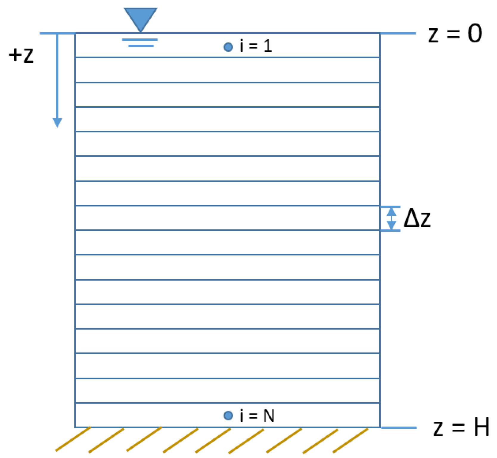
In Equations (19) and (20), $\mathsf{\Delta }z$ is the model grid spacing and the subscript $i$ refers to the model grid cell of interest (Figure 1). The superscripts refer to time in the simulation, where time $n+1$ is one timestep in the future from time $n$, and $\mathsf{\Delta }t$ is the model timestep. The source-sink term of Equation (18) is represented by ${\mu }_{net}$ and includes the effects of population growth, mortality, excretion, and respiration.

In a particle-tracking framework, the location of an organism or colony, represented by a particle, is calculated at each timestep. The numerical solution for a model of cyanobacteria depth for a particle, $z_p$, was computed using

$$z_{p_i}^{n+1}=z_{p_i}^n+v_{p_i}^n\mathsf{\Delta }t+R\sqrt{6D_{z_i}^n\mathsf{\Delta }t}$$

(21)

where the subscript $i$ refers to the particle of interest, the superscript $n$ refers to the time in the simulation, and $\mathsf{\Delta }t$ is the model timestep [45]. The third term on the right-hand side includes a random number, $R$, from a uniform distribution between $-1$ and $1$, and represents the variation in motion among particles due to turbulent diffusion. Particles that were predicted to move past the bed ($z=H$) during a displacement were instead assigned a location equal to one half of a grid cell height above the bed. Particles that were predicted to move past the surface ($z=0$) during a displacement were assigned a location equivalent to the surface.

2.1.1. Predefined Velocity

A simple way to model the vertical movement of cyanobacteria is to assume a velocity function for colonies based on knowledge of their typical movement. Because cyanobacteria vertical migration is due to buoyancy regulation, which is dependent on light, a velocity function that represents changes in light is a logical choice.

If cyanobacteria colonies are assumed to migrate vertically on a daily cycle, an equation for colony velocity as a function of time can be used, i.e.,

$$v_p\left(t\right)=A\frac{2\pi }{86,400\mathrm{s}}cos\left(\frac{2\pi }{86,400\mathrm{s}}t+\varphi \right)$$

(22)

Here, $A$ is migration amplitude and the period is assumed to be one day (86,400 s). The value of the phase ($\varphi$) depends on the initial location of colonies. For example, if $t=0$ in the simulation corresponds to midnight and colonies are assumed to be at the bottom at that time, the value of the phase is $\frac{\pi }{2}$ with positive velocity corresponding to downward movement (Figure 1).

A slightly more complex approach is to assume a velocity function that is dependent on space as well as time, as in Belov and Giles [4]. Modifying Equation (13) to use the same notation as Equation (22) gives:

$$v_p\left(t,z\right)=\{\begin{array}{c}A\frac{2\pi }{86,400\mathrm{s}}cos\left(\frac{2\pi }{86,400\mathrm{s}}t+\varphi \right)e^{-\alpha C\left(H-z\right)},I_0>0\\ A\frac{2\pi }{86,400\mathrm{s}}cos\left(\frac{2\pi }{86,400\mathrm{s}}t+\varphi \right),\hspace{1em}\hspace{1em}\hspace{1em}{I}_0\le 0\end{array}$$

(23)

Here, $\alpha$ is the light attenuation coefficient and $I_0$ is solar irradiance at the water surface. The addition of the exponential term gives colonies deeper in the water column higher speeds and responds to variations in water clarity when the light attenuation coefficient, $\alpha$, is variable. A calibration coefficient, $C$, is included in the light attenuation exponent term because the light attenuation coefficient used in the original study was 0.1 ${\mathrm{m}}^{-1}$, which is lower than values often found in lakes and reservoirs. In the original study, the light attenuation coefficient was assumed to be constant and the exponential term was applied whether or not there was irradiance at the water surface. Here, the exponential term is only applied during the photoperiod so that the effects of water clarity are only included when there is sunlight present. During dark periods, the equation reduces to Equation (22). Tables S1 and S2 in Supplementary Materials summarize equations for continuum and particle tracking modeling frameworks.

2.1.2. Dynamic Velocity

The predefined velocity approaches can predict cyanobacteria movement based on the observed tendency of colonies to migrate vertically on a daily cycle; however, they do not reflect the response of colonies to variations in solar irradiance. In order to capture this natural behavior, colony velocity was also calculated based on relationships between sunlight and cyanobacteria growth and colony density. Using this approach, the change in cyanobacteria colony density was computed based on the solar irradiance at the surface of the water and the colony’s depth in the water column. This density was then used to solve for the colony’s settling velocity via Stokes’ law Equation (2). Three different approaches were tested to model cyanobacteria buoyancy change: a model based on growth kinetics, the model from Visser et al. [13], and a model that incorporates light response and calibration coefficients.

The first dynamic velocity model described here is the growth kinetics model. Because cyanobacteria buoyancy regulation is controlled by the accumulation and depletion of photosynthetic products, changes in cell and colony density follow similar patterns to algal growth kinetics [39]. Assuming that the change in colony density can be calculated based on the net growth rate (${\mu }_{net}$), the change in cyanobacteria colony density (${\rho }_c$) is given by

$$\frac{\partial {\rho }_c}{\partial t}={\mu }_{net}{\rho }_c$$

(24)

The net growth rate for cyanobacteria in this case is given by

$${\mu }_{net}={\mu }_{g,max}F\left(I\right)-{\mu }_r-{\mu }_e-{\mu }_m$$

(25)

where ${\mu }_{g,max}$ is the maximum growth rate, ${\mu }_r$ is the respiration rate, ${\mu }_e$ is the excretion rate, and ${\mu }_m$ is the mortality rate of the cyanobacteria species. A function of light, $F\left(I\right)$, scales the maximum growth rate and is given by the Steele equation [46], which accounts for photoinhibition at high irradiance values, i.e.,

$$F\left(I\right)=\frac{I}{I_s}{e}^{-\frac{I}{I_s}+1}$$

(26)

Here, $I$ is irradiance at the location of interest and $I_s$ is the saturating light intensity for the cyanobacteria species. Irradiance at the depth of the colony is found from

$$I\left(z\right)=\left(1-\beta \right)I_0{e}^{-\alpha z}$$

(27)

where $\beta$ is the fraction of solar irradiance absorbed at the water surface, and $\alpha$ is the light attenuation coefficient [47].

In the particle-tracking framework, the density of each cyanobacteria colony was calculated along with its location at each timestep. Solving Equation (24) for the density of colony $i$ at time $n+1$ gives

$${\rho }_{c_i}^{n+1}={\rho }_{c_i}^n{\mu }_{ne{t}_i}^n\mathsf{\Delta }t+{\rho }_{c_i}^n$$

(28)

where ${\mu }_{ne{t}_i}^n$ is calculated at the location of the colony at time $n$. The velocity of the colony was then found using Stokes’ law Equation (2) and substituted into Equation (21) to determine the colony’s new position.

Applying a light-driven density change to colonies in a continuum framework requires a different approach than in a particle-tracking framework. In the particle-tracking framework, colonies are followed throughout the simulation and their densities are cumulative from the start of the simulation. In a continuum framework, there is no distinction between colonies and therefore no way to track each colony’s density change over time. To overcome this, colony density change was determined for each model grid cell using Equation (28), with the subscript $i$ now referring to the grid cell of interest rather than the particle of interest. The colony velocity for each grid cell was found using Stokes’ law as in the particle-tracking framework Equation (2).

In this case, the numerical scheme for solving Equation (18) differs from Equations (19) and (20) because velocities in neighboring grid cells can have opposite directions. Hence, the general form for the solution of Equation (18) is

$$c_i^{n+1}=\frac{D_z\mathsf{\Delta }t}{\mathsf{\Delta }{z}^2}\left(c_{i+1}^n-2c_i^n+c_{i-1}^n\right)-\frac{\mathsf{\Delta }t}{\mathsf{\Delta }z}\left(\left|v_{p_i}^n{c}_i^n\right|-v_{p_B}^n{c}_{i+1}^n-v_{p_T}^n{c}_{i-1}^n\right)+\left({\mu }_{net}\mathsf{\Delta }t+1\right)c_i^n$$

(29)

Here, $v_{c_B}$ and $v_{c_T}$ are the velocities of colonies entering grid cell $i$ from above and below, respectively, such as

$$v_{p_B}^n=\{\begin{array}{c}{v}_{p_{i+1}}^n,v_{p_{i+1}}^n<0\\ 0,\hspace{1em}\hspace{0.17em}{v}_{p_{i+1}}^n\ge 0\end{array}$$

(30)

$$v_{p_T}^n=\{\begin{array}{c}{v}_{p_{i-1}}^n,v_{p_{i-1}}^n>0\\ 0,\hspace{1em}\hspace{0.17em}{v}_{p_{i+1}}^n\le 0\end{array}$$

(31)

An adjustment is required for calculating $F\left(I\right)$ using the continuum framework because light intensity will vary across the grid cell due to light attenuation with depth. To reflect this, the integral of light over the grid cell is used and $F\left(I\right)$ becomes [46]:

$$F\left(I\right)=\frac{e}{\alpha \mathsf{\Delta }z}\left[e^{-{\gamma }_2}-e^{-{\gamma }_1}\right]$$

(32)

where

$${\gamma }_1=\frac{\left(1-\beta \right)I_0}{I_s}{e}^{-\alpha \left(i-1\right)\mathsf{\Delta }z}$$

(33)

$${\gamma }_2=\frac{\left(1-\beta \right)I_0}{I_s}{e}^{-\alpha \left(i\right)\mathsf{\Delta }z}$$

(34)

While the above continuum framework accounts for changes in colony density due to the instantaneous growth rate, it does not include the same information about past growth as the particle-tracking framework. To address this, an exponentially-decaying, weighted average of past growth rates in each grid cell was applied to the same continuum framework outlined above as

$${\rho }_{c_i}^{n+1}=\frac{{{\displaystyle \sum }}_{q=-1}^Q{\rho }_{c_i}^{n-q}{W}^q}{{{\displaystyle \sum }}_{q=-1}^Q{W}^q}$$

(35)

Here, the past densities in the grid cell $i$ are multiplied by a weight $W$ and summed. The total number of timesteps over which to average past densities is given by $Q$. The weight decreases exponentially with time before the present, so that densities predicted at more recent timesteps have greater weights, i.e.,

$$W^q=e^{-k\left(t^{n+1}-t^{n-q}\right)}$$

(36)

Here, $k$ is the time decay constant for influence of past densities. This is similar to the approach taken by Serizawa et al. [39], shown in Equations (14) and (15).

The equations from Visser et al. [13], Equations (9) and (10), were also applied to both the continuum and particle-tracking frameworks using Equations (37) and (38), respectively. A correction factor, ${\rho }_{*}$, was applied to Equation (10) to reflect the difference between the buoyant density modeled here and the non-buoyant density on which the equations in that study were based. Hence, the updated equations used were

$$I_i^n\ge I_c,{\rho }_{c_i}^{n+1}=(c_{1}I{e}^{-I/I_0}+c_2)\mathsf{\Delta }t+{\rho }_{c_i}^n$$

(37)

$$I_i^n<I_c,{\rho }_{c_i}^{n+1}=(f_1({\rho }_{i_i}^n+{\rho }_{*})+f_2)\mathsf{\Delta }t+{\rho }_{c_i}^n$$

(38)

It was assumed that ${\rho }_i$ was the last density experienced by a particle or grid cell while the irradiance was greater than $I_c$, the compensation irradiance. For example, at dawn ${\rho }_i$ for a particle or grid cell is the density of that particle or grid cell during the last timestep at the end of the previous day during which it experienced an irradiance greater than $I_c$. If a particle moves to a location where the light intensity is less than $I_c$, or if the light intensity at a particle’s location or in a grid cell becomes less than $I_c$ over time, ${\rho }_i$ is the last density of that particle or grid cell before light intensity changed. In the continuum framework, light intensity was averaged across a grid cell depth using

$$I_i=\frac{I_0\left(1-\beta \right)}{-k\mathsf{\Delta }z}\left(e^{-\alpha z_i}-e^{-\alpha z_{i-1}}\right)$$

(39)

The parameter values used in Visser et al. [13] were converted from units of $\mathsf{\mu }\mathrm{mol}\mathrm{photon}{\mathrm{s}}^{-1}$ to $Watts$ [48] (Table S3 in Supplementary Materials).

An adjustment was made to the Visser et al. [13] model to account for adaptations from the particle-tracking to the continuum framework. If the calculated value of ${\rho }_i$, the density used to calculate density decrease in the dark, is below a minimum value, it was increased to that minimum value. This density then varies with depth using

$${\rho }_{i_i}={\rho }_{i_S}+\left({\rho }_{i_B}-{\rho }_{i_S}\right)\left(\frac{z_i}{H}\right)$$

(40)

where ${\rho }_{i_S}$ is the minimum allowable value of ${\rho }_i$ at the surface and ${\rho }_{i_B}$ is the minimum allowable value at the bed.

A third approach to modeling light-dependent density change was based on the above two approaches, as well as the model of Kromkamp and Walsby [8]. In both Visser et al. [13] and Kromkamp and Walsby [8], density increases were modeled using equations similar to growth kinetics equations with additional calibration coefficients. In Kromkamp and Walsby [8], a Monod-type equation was used to model density increase with light and a linear relationship was used to model density decrease in the dark Equation (1). In Visser et al. [13], density increases were modeled using an exponential term which accounts for photoinhibition and density decreases were modeled with a linear term. In the light function buoyancy model described here, density change was assumed to follow the same response to light as growth kinetics, including photoinhibition. However, calibration coefficients $c_1$ and $c_2$ are used rather than the growth rates described above, and growth is assumed to be zero-order rather than first-order, i.e.,

$$\frac{\partial \rho }{\partial t}=c_{1}F\left(I\right)-c_2$$

(41)

This allows density change to be calculated separately from population growth while still representing the relationship between density change and light. In the absence of light, density decreases at a constant rate. The numerical solution for Equation (41) is given by

$${\rho }_{c_i}^{n+1}=\left(c_{1}F\left(I_i^n\right)-c_2\right)\mathsf{\Delta }t+{\rho }_{c_i}^n$$

(42)

A summary of model equations is shown in Tables S4 and S5 in Supplementary Materials for the continuum and particle tracking frameworks, respectively.

2.2. Field Data

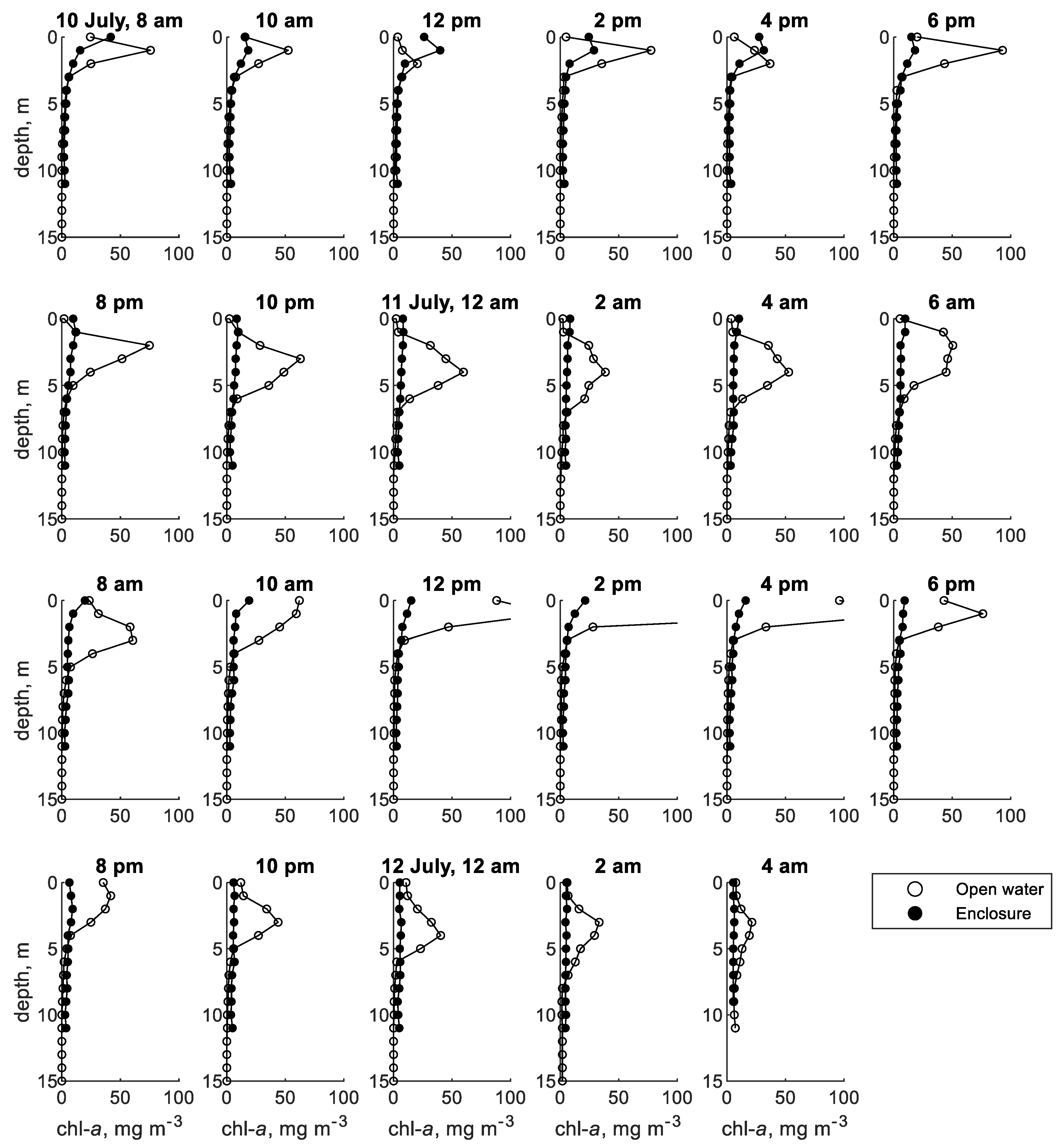
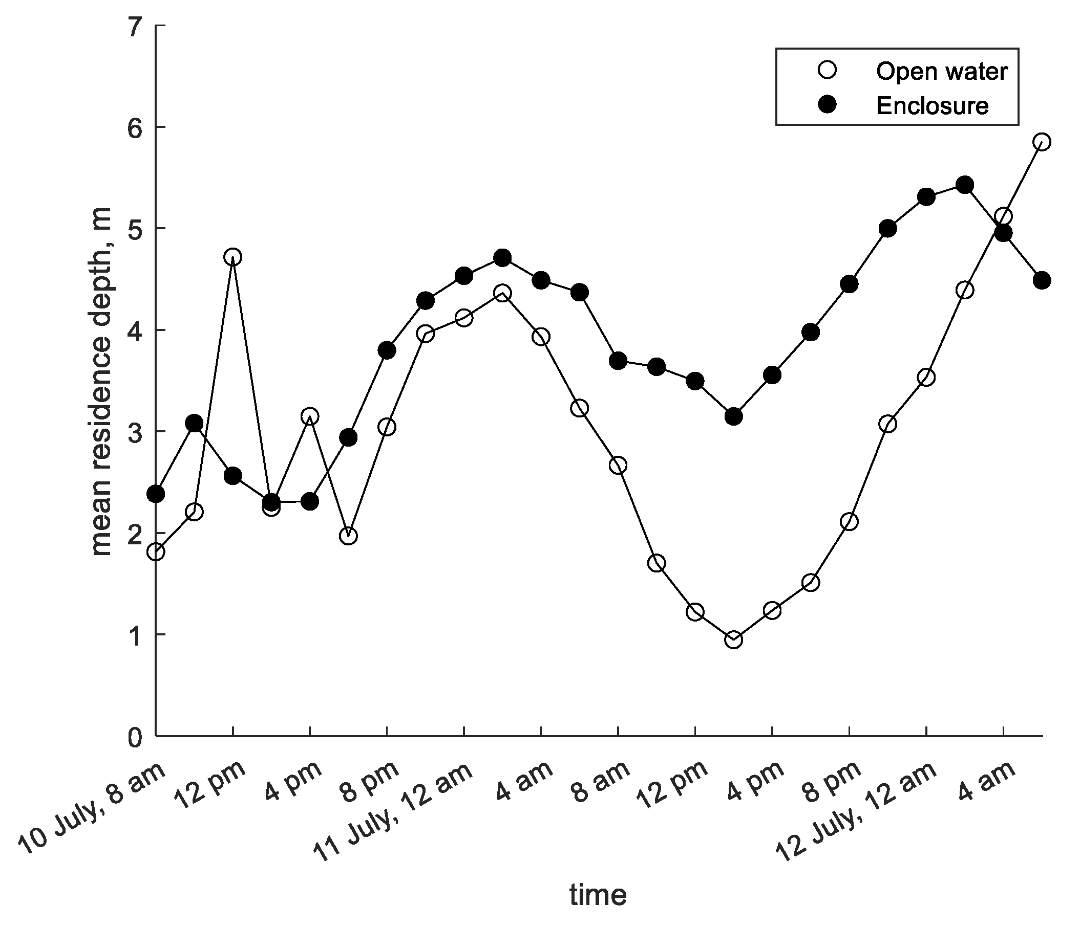
The models of cyanobacteria vertical migration described in Section 2.1 were tested using data from two published field studies. The first is a study by Cui et al. [12] conducted in Shennong Stream, a tributary of the Yangtze River in the Three Gorges Reservoir complex in China’s Hubei Province. Water samples were taken at depth intervals of 1 m every two hours on 10–12 July 2014, and analyzed for chlorophyll a concentration (Figure 2). Additional samples taken near the surface, at mid-depth, and near the bed were analyzed for phytoplankton species composition, which indicated that almost 90% of the phytoplankton in the study areas belonged to the cyanobacteria genus Microcystis. This provided a basis for using chlorophyll a concentration to approximate Microcystis concentration. Two study sites were sampled: an 11 m-deep site in an enclosure protected from water currents and a 15 m-deep area in the open water. The published study includes solar irradiance measurements, calculated light attenuation coefficients, chlorophyll a concentration profiles, and calculated mean residence depth (MRD) of chlorophyll a concentration at two-hour sampling intervals (Figure 3).

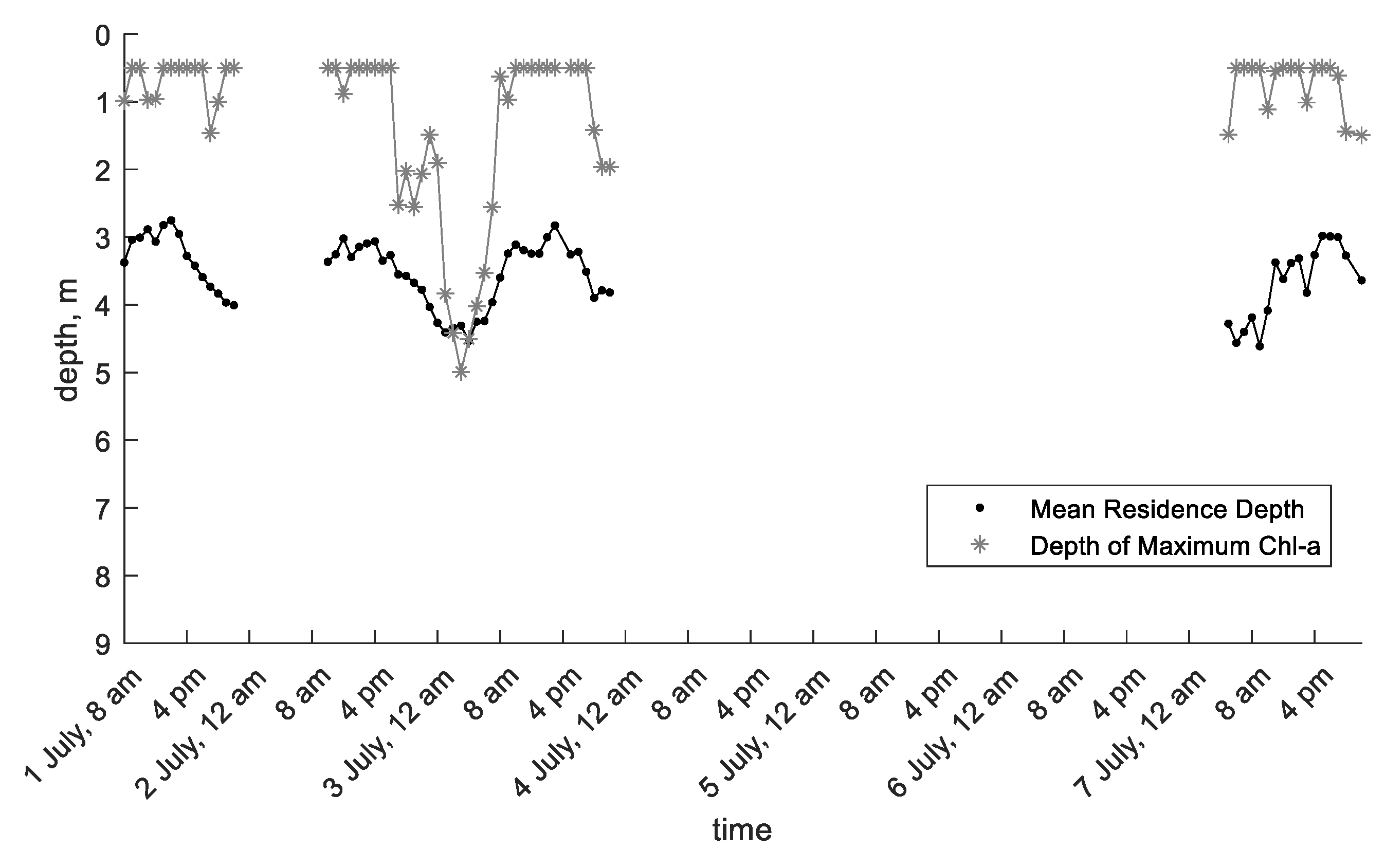
The second data set is from a study by Wang et al. [49] conducted in another part of the Three Gorges Reservoir, Xiangxi Bay. In this study, hourly chlorophyll a measurements were taken at depth intervals of 0.5 m from 0.5 m below the surface to a depth of 9 m on 1 July, 2–3 July, and 7 July 2008. On 3 July, water samples were taken at six different depths and analyzed for phytoplankton species composition. The results showed that 49.0–83.2% of phytoplankton biomass (mg/L) and 83.7–94.8% of phytoplankton density (10⁷ cells/L) was due to Microcystis aeruginosa. Solar irradiance measured at the surface was recorded every hour. Calculated MRD and depth of maximum chlorophyll a concentration were also reported in the published study (Figure 4).

2.3. Model Setup

In all models, a grid cell height ($\mathsf{\Delta }z$) of 0.2 m was used and the model timestep ($\mathsf{\Delta }t$) was 60 s. Water current was not modeled, and water was assumed to be quiescent. Chlorophyll a concentration was used as a proxy for Microcystis concentration. Parameter values for models were chosen from within reasonable ranges based on the literature (

Table 2. Literature values for biological parameters of cyanobacteria used in models.

Study	Identifier	Minimum Density, $\mathbf{kg}{\mathbf{m}}^{\mathbf{-}\mathbf{3}}$	Maximum Density, $\mathbf{kg}{\mathbf{m}}^{\mathbf{-}\mathbf{3}}$	Colony Radius, $\mathsf{\mu }\mathbf{m}$	Saturating Light Intensity, $\mathbf{W}{\mathbf{m}}^{\mathbf{-}\mathbf{2}}$	Maximum Growth Rate, ${\mathbf{day}}^{\mathbf{-}\mathbf{1}}$
Reynolds [50]	-	-	-	25–1000	-	-
Reynolds et al. [51]	cyanobacteria	-	-	-	-	0.6–0.8
	M. aeruginosa	985	1005	120–3200	-	-
	A. flos-aqua	920	1030	28–100	-	-
	P. agardhii	985	1085	13.7–18.3	-	-
Nakamura et al. [52]	Microcystis sp.	-	-	10–300	-	-
Visser et al. [13]	Microcystis sp.	-	-	-	139	-
Long et al. [53]	M. aeruginosa	-	-	-	-	1.2
Wu and Song [54]	M. aeruginosa	-	-	-	119–244	-
Wu et al. [55]	M. aeruginosa	-	-	-	65–119	-
Zhang et al. [56]	M. aeruginosa	-	-	-	75–392	-
Zhu et al. [17,57]	Microcystis sp.	967	997	10–350	-	-
Rowe et al. [58]	Microcystis sp.	-	-	12.5–370, median: 58.5	-	-

) and calibrated for each model (

Table 3. Ranges of values used in model applications to field study data.

Variable	Description	Value Range
A, m	Migration amplitude	0.2–1.23
$\varphi$, rad	Phase offset	$\pi$
$C$	Light attenuation calibration coefficient	0.05–0.13
${\mu }_{g,max},{\mathrm{day}}^{-1}$	Maximum growth rate	0.7–1.0
${\mu }_m,{\mathrm{day}}^{-1}$	Mortality rate	0.06–0.25
${\mu }_e,{\mathrm{day}}^{-1}$	Excretion rate	0.04
${\mu }_r,{\mathrm{day}}^{-1}$	Respiration rate	0.04
$I_s,\mathrm{W}{\mathrm{m}}^{-2}$	Saturating light intensity	100–150
$c_1,{\mathrm{day}}^{-1}$	Coefficient of density increase for light function model	0.00545–0.02
$c_2,{\mathrm{day}}^{-1}$	Coefficient of density decrease for light function model	0.00145–0.00518
$r_c,\mathsf{\mu }\mathrm{m}$	Colony radius	15–64
${\rho }_{min},\mathrm{kg}{\mathrm{m}}^{-3}$	Minimum colony density	920–980
${\rho }_{max},\mathrm{kg}{\mathrm{m}}^{-3}$	Maximum colony density	140–185
${\rho }_{0,S},\mathrm{kg}{\mathrm{m}}^{-3}$	Initial colony density at surface	930–1080 (continuum) 920–980 (particles)
${\rho }_{0,B},\mathrm{kg}{\mathrm{m}}^{-3}$	Initial colony density at bed	930–980 (continuum) 995–1010 (particles)
${\rho }_{i,S},\mathrm{kg}{\mathrm{m}}^{-3}$	Minimum initial colony density at surface for Visser et al. [13] model	980–1080
${\rho }_{i,B},\mathrm{kg}{\mathrm{m}}^{-3}$	Minimum initial colony density at bed for Visser et al. [13] model	975–980
${\rho }_{*},\mathrm{kg}{\mathrm{m}}^{-3}$	Correction for density decrease equation for Visser et al. [13] model	67
$k,{\mathrm{day}}^{-1}$	Time decay constant for averaging past densities	5

).

In dynamic velocity models, colonies were assumed to have a minimum and maximum allowable density (${\rho }_{min}$ and ${\rho }_{max}$, respectively). When predicted densities were greater than the maximum or less than the minimum allowed values, the value was set to ${\rho }_{max}$ or ${\rho }_{min}$, respectively. It was also necessary to define initial densities (${\rho }_0$) for all colonies (particle-tracking) or colonies within a grid cell (continuum). Initial colony density, ${\rho }_{0_i}$ was assumed to vary exponentially from the surface to the bed, following a similar pattern to light decay with depth, as

$${\rho }_{0_i}={\rho }_{0_S}+\left({\rho }_{0_B}-{\rho }_{0_S}\right)\left(1-e^{-z_i}\right)$$

(43)

where ${\rho }_{0_S}$ is the initial colony density at the surface and ${\rho }_{0_B}$ is the initial colony density at the bed. In the particle-tracking framework, the number of particles in each control volume corresponding to a model grid cell, $P_i$, was determined based on the initial concentration in the model grid cell, $c_{0_i}$, and initial densities of colonies in the control volume as

$$P_i=\frac{c_{0_i}\mathsf{\Delta }zBx}{\mathrm{K}{\rho }_{c_0}\frac{4}{3}\pi r_c^3}$$

(44)

where $r_c$ is colony radius, $B$ and $x$ are the lateral and longitudinal dimensions of the model grid, respectively, and $\mathrm{K}$ is the number of cyanobacteria colonies represented by one model particle. This term was included to reduce the number of particles needed and computation time. Both $r_c$ and the total number of particles were kept constant throughout a simulation.

In the continuum framework, population growth and decay were represented by the source-sink term from Equation (18). In the particle-tracking framework, the growth equations were applied to the population density of each particle. This was computed separately from the buoyant density of colonies so that minimum and maximum allowable colony densities used in velocity calculations did not affect population values.

In order to compare results from models in the particle-tracking framework to those from models in the continuum framework, concentration predicted in the particle-tracking framework was computed for control volumes corresponding to each model grid cell as

$$c_i^n=\frac{\frac{4}{3}\pi r_c^3{\displaystyle \sum }{\rho }_c}{\mathsf{\Delta }zBx}$$

(45)

where ${\displaystyle \sum }{\rho }_c$ is the sum of population densities of colonies within the control volume.

Input data for the Shennong Stream models included solar irradiance at the water surface and light attenuation coefficients calculated in the original study. Initial conditions were assumed to be the first recorded field measurement at each depth, taken at 08:00 a.m. on the first day of the study. This also determined the simulation start time. The vertical diffusion coefficient ($D_z$) was set to a constant ${10}^{-5}{\mathrm{m}}^2{\mathrm{s}}^{-1}$ in the enclosure site and ${10}^{-4}{\mathrm{m}}^2{\mathrm{s}}^{-1}$ in the open water site in order to represent the differences in turbulent mixing between the two sites.

Absolute mean errors (AMEs) of all models compared to field data were calculated for each of the metrics. Predictions of chlorophyll a concentration were prioritized over predictions of MRD during calibration. The amount of cyanobacteria (represented by chlorophyll a) at each depth in the water column is of interest here because it is a primary measurement of cyanobacteria distribution, while MRD is a derived metric. Chlorophyll a concentration errors are averages of AMEs from chlorophyll a concentration profiles. Inputs for the Xiangxi Bay field study application were solar irradiance measured at the water surface and initial chlorophyll a concentrations at 0.5 m depth intervals (Figure 4), both reported in the study published by Wang et al. [49]. Quantitative model-data comparisons were made with hourly MRD and depth of maximum chlorophyll a concentration reported in the study. Similar to the Shennong Stream study, predictions of depth of maximum chlorophyll a concentration were prioritized over predictions of MRD.

The light attenuation coefficient was set to 0.5 m⁻¹ for all models of Xiangxi Bay. This was done in part to test the models with a lower light attenuation coefficient value, as the values in the Shennong Stream study were relatively high. Each model was run with two different values of $D_z$,${10}^{-5}{\mathrm{m}}^2{\mathrm{s}}^{-1}$ and ${10}^{-4}{\mathrm{m}}^2{\mathrm{s}}^{-1}$.

3. Modeling Results

3.1. Shennong Stream Enclosure

The chlorophyll a profiles measured in the enclosure site in Shennong Stream show subtle changes in shape throughout the study period (Figure 2). A subsurface peak can be seen on the morning of the first day; after that, the profile becomes more uniform and then develops a surface maximum on the morning of the second day. The MRD shows a distinct diurnal sinusoidal pattern over time with an amplitude of approximately 1.5 m (Figure 3).

In the continuum modeling framework, the two predefined velocity models resulted in the lowest AME values for both MRD and chlorophyll a concentration for the enclosure site (

Table 4. Error statistics for models of Shennong Stream enclosure site.

	Mean Residence Depth AME, m		Chlorophyll a Concentration (Profile Average) AME, mg m3
Model	Continuum	Particle Tracking	Continuum	Particle Tracking
Time-varying velocity	1.074	1.127	2.871	3.176
Belov and Giles [4]	0.799	0.795	2.549	2.796
Growth kinetics	1.348	0.613	3.446	3.925
Growth kinetics with time decay	1.318	-	3.271	-
Visser et al. [13]	1.338	0.772	3.378	3.205
Light function	1.359	0.599	3.522	3.273
Light function with time decay	1.252	-	3.201	-

). These models were able to represent the sinusoidal pattern of the MRD seen in the field data (Figure 5). The dynamic velocity models did not predict MRD as well as the predefined velocity models. In most of the dynamic velocity models, the MRD did not show the distinct sinusoidal pattern seen in the data and instead showed little variation over time (Figure S2 in Supplementary Materials). The predefined velocity models also captured chlorophyll a concentration profiles better than the dynamic velocity models at this site (Figures S3 and S4 in Supplementary Materials). Most of the dynamic velocity models failed to predict concentration deeper in the water column the second day, with the exception of the light function model with time decay (Figure S4 in Supplementary Materials).

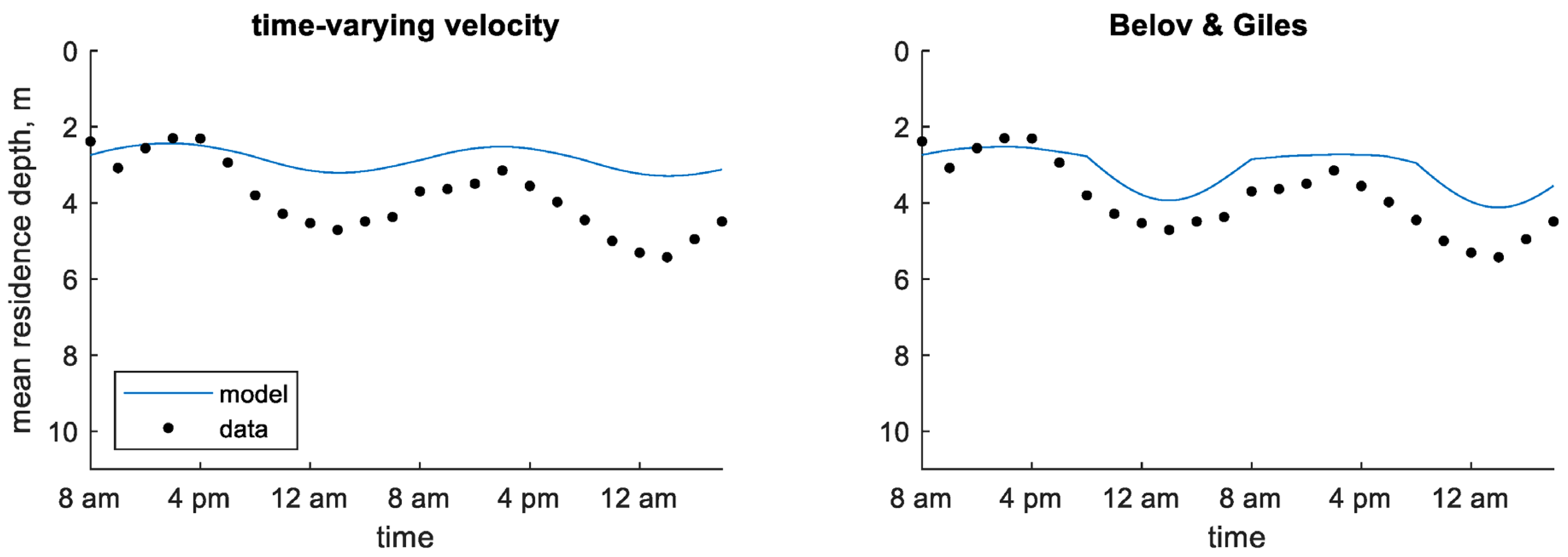
Somewhat different results were obtained from models applied to the Shennong Stream enclosure site using the particle-tracking framework. Among these models, MRD was best predicted by the dynamic velocity models, especially the light function and growth kinetics models (Table 4). However, the predefined velocity models still follow the correct shape of the MRD over the entire study period (Figure S5 in Supplementary Materials), while the dynamic velocity models tend to under-predict the MRD during the final several hours (Figure S6 in Supplementary Materials). As with models in the continuum framework, chlorophyll a was best predicted by the Belov and Giles [4] model. In the vertical concentration time-series plots, the predefined velocity models show more diffusion than the dynamic velocity models (Figures S7 and S8 in Supplementary Materials).

The most notable difference between the continuum and particle-tracking frameworks for this study can be seen in the dynamic velocity models. These models resulted in AMEs of 1.25–1.36 m for MRD in the continuum framework and 0.60–0.77 m in the particle-tracking framework (Table 4). Little change was seen in chlorophyll a concentration predictions by dynamic velocity models or MRD predictions by predefined velocity models. However, AMEs for chlorophyll a concentration predictions by predefined velocity models increased from 2.55 and 2.87 mg/m³ in the continuum framework to 2.80 and 3.18 mg/m³ in the particle-tracking framework.

3.2. Shennong Stream Open Water

In the open water site in Shennong Stream, concentration profile plots showed a more distinct shape, alternating between a subsurface peak and a surface maximum (Figure 2). As in the enclosure site, MRD generally followed a sinusoidal pattern. However, in the open water MRD moved closer to the surface on the second morning and continued to move downward at the end of the study period when the MRD in the enclosure had begun moving upward (Figure 3).

Of the models in the continuum framework, the dynamic velocity models predicted both MRD and chlorophyll a profiles better than the predefined velocity models, though only slightly (

Table 5. Error statistics for models of the Shennong Stream open water site.

	Mean Residence Depth AME, m		Chlorophyll a Concentration (Profile Average) AME, mg m3
Model	Continuum	Particle Tracking	Continuum	Particle Tracking
Time-varying velocity	1.129	1.097	8.589	8.654
Belov and Giles [4]	1.113	1.100	8.645	8.716
Growth kinetics	1.096	0.986	7.735	8.498
Growth kinetics with time decay	1.064	-	7.193	-
Visser et al. [13]	1.093	0.993	7.589	8.670
Light function	1.087	0.964	7.425	8.654
Light function with time decay	1.087	-	7.253	-

). However, a visual inspection of the MRD predictions shows that the dynamic velocity models predict an almost constant MRD, while the predefined velocity models perform better at capturing the shape of the MRD over time (Figures S9 and S10 in Supplementary Materials). The concentration time-series plots of chlorophyll a show that concentration predictions are less diffuse than in the enclosure site, and the predefined velocity models predict that chlorophyll a is more diffuse than the field data (Figure S11 in Supplementary Materials). The dynamic velocity models do not show as much of a change in diffusion after adjusting the vertical diffusion coefficient for the open water site, resulting in more accurate profile predictions (Figure S12 in Supplementary Materials).

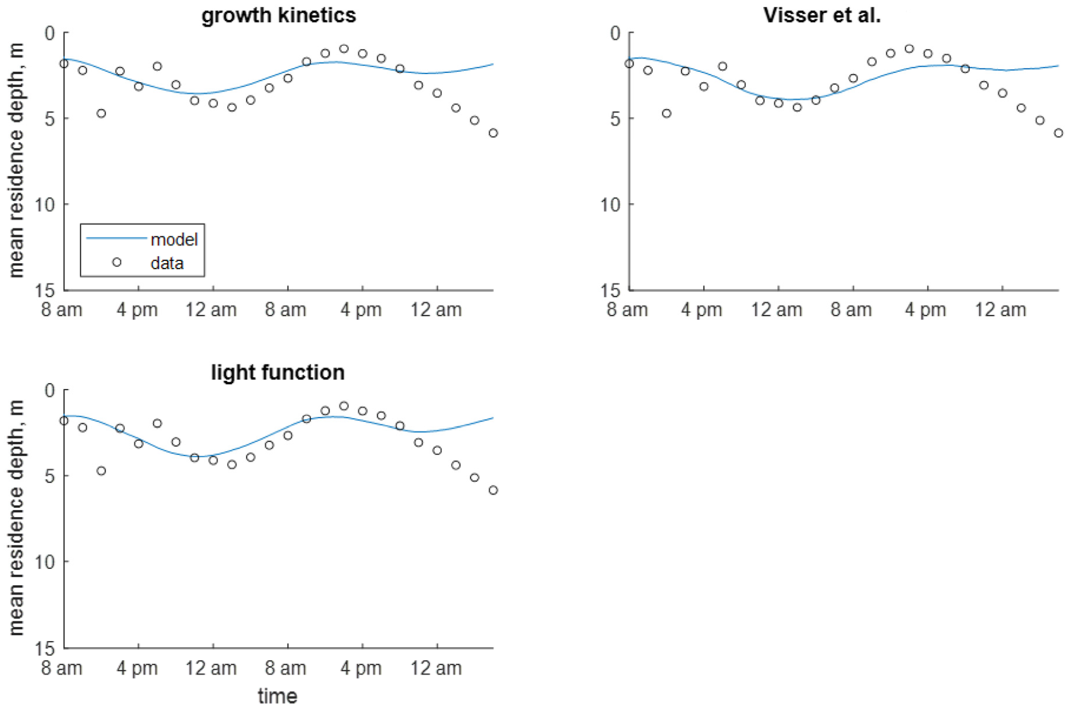
Results for the open water site using the particle-tracking framework did not show much variation across models. Dynamic velocity models resulted in lower error statistics than predefined velocity models, though only slightly (Table 5). Results were mixed for chlorophyll a concentration error statistics; the growth kinetics model gave the lowest error, while the light function model gave the highest. Visual inspection of the MRD plots suggest that all models captured the general shape of the sinusoid curve, although on the second day the predefined velocity models start to predict a deeper MRD than observed while the dynamic velocity models predict too shallow an MRD (Figure 6 and Figure S13 in Supplementary Materials). The dynamic velocity models better reflect the level of chlorophyll a diffusion seen in the observed data than do the predefined velocity models (Figures S15 and S16 in Supplementary Materials).

Error statistics for MRD were again lower for dynamic velocity models in the particle-tracking framework compared to the continuum framework. However, the difference was not as much as seen in the models of the enclosure site, decreasing from 1.06–1.10 m to 0.96–0.99 m (Table 5). Errors in chlorophyll a concentration predictions by dynamic velocity models increased from 7.19–7.73 mg/m³ in the continuum framework to 8.50–8.67 mg/m³ in the particle-tracking framework. Differences between frameworks were smaller for both metrics in predefined velocity models.

3.3. Xiangxi Bay

Chlorophyll a contours from Xiangxi Bay show steep concentration gradients during the late morning and afternoon and more vertical diffusion in the middle of the night, possibly from convective night-time cooling [49]. The depth of maximum chlorophyll a concentration is near the surface on 1 July and 7 July and during the middle of the day on 2–3 July. It moves down to approximately 5 m deep on the early morning on 3 July. MRD shows a sinusoidal pattern over time that reaches maximum depths in the middle of the night and shallow depths in the afternoon (Figure 4).

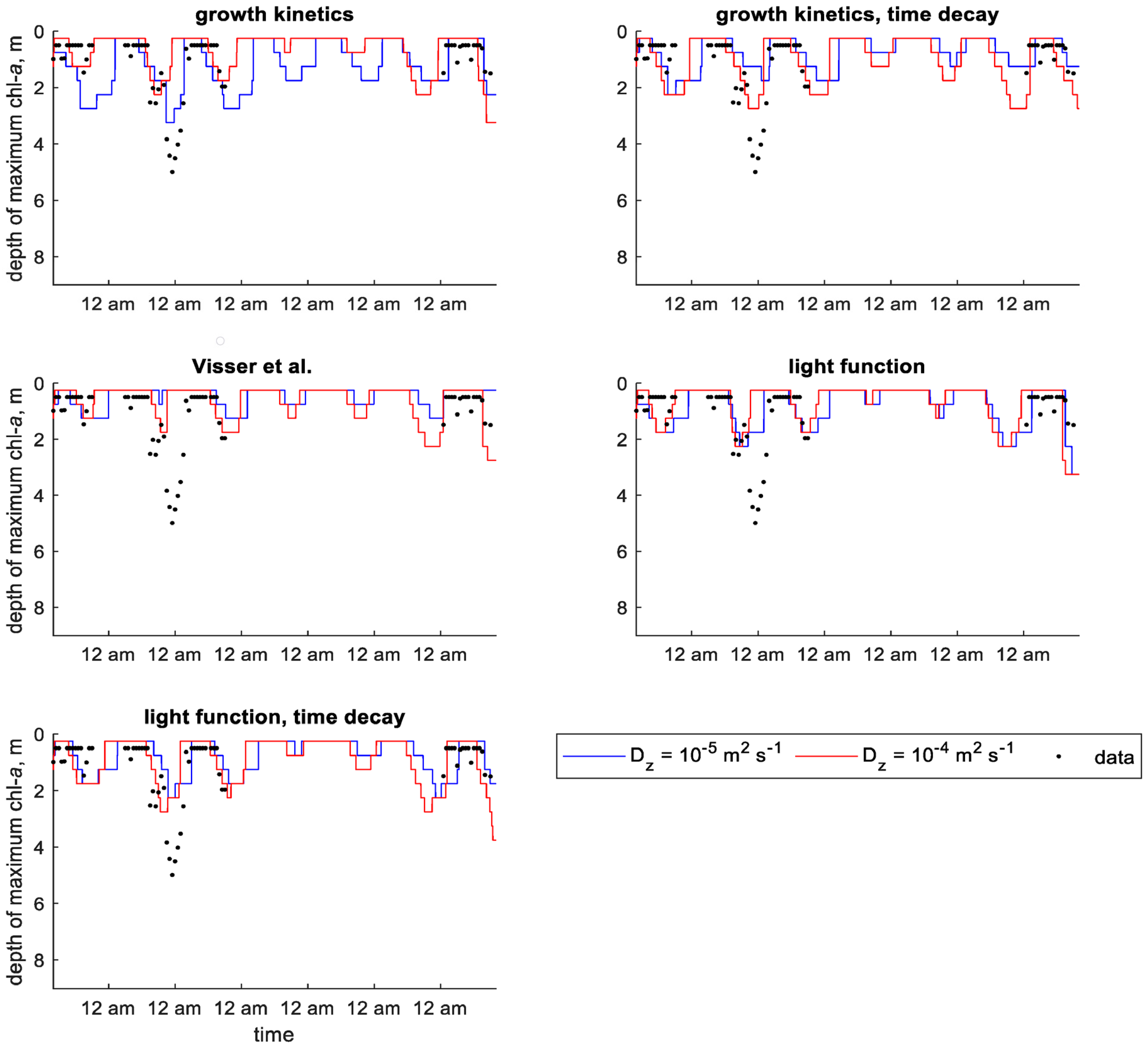
Within the continuum framework, the predefined velocity models resulted in better error statistics than did the dynamic velocity models using a $D_z$ value of 10⁻⁵ m² s⁻¹ (

Table 6. Error statistics for models of Xiangxi Bay.

	Mean Residence Depth AME, m				Depth of Maximum Chlorophyll a Concentration AME, m
	Dz = 10−5 m2 s−1		Dz = 10−4 m2 s−1		Dz = 10−5 m2 s−1		Dz = 10−4 m2 s−1
Model	Continuum	Particle Tracking	Continuum	Particle Tracking	Continuum	Particle Tracking	Continuum	Particle Tracking
Time-varying velocity	0.351	0.509	0.422	0.415	0.557	0.609	0.696	0.846
Belov and Giles [4]	0.380	0.585	0.409	0.413	0.561	0.554	0.680	0.844
Growth kinetics	1.201	0.595	0.672	0.461	0.641	1.598	0.744	1.373
Growth kinetics with time decay	1.299	-	0.395	-	0.730	-	0.667	-
Visser et al. [13]	1.287	1.001	0.374	0.392	0.877	2.800	0.754	1.598
Light function	1.410	0.887	0.629	0.371	0.693	1.837	0.802	1.454
Light function with time decay	1.650	-	0.426	-	0.725	-	0.687	-

). In plots of MRD, these models reproduced the pattern seen in the field data (Figure S17 in Supplementary Materials), while the dynamic velocity models predicted a more shallow MRD than that seen in the data (Figure S18 in Supplementary Materials). The predefined velocity models also show more accurate predictions of depth of maximum chlorophyll a concentration when it is at its deepest between July 2 and 3 (Figure S19 in Supplementary Materials). Most of the dynamic velocity models do not correctly predict this, with the exception being the growth kinetics model (Figure 7).

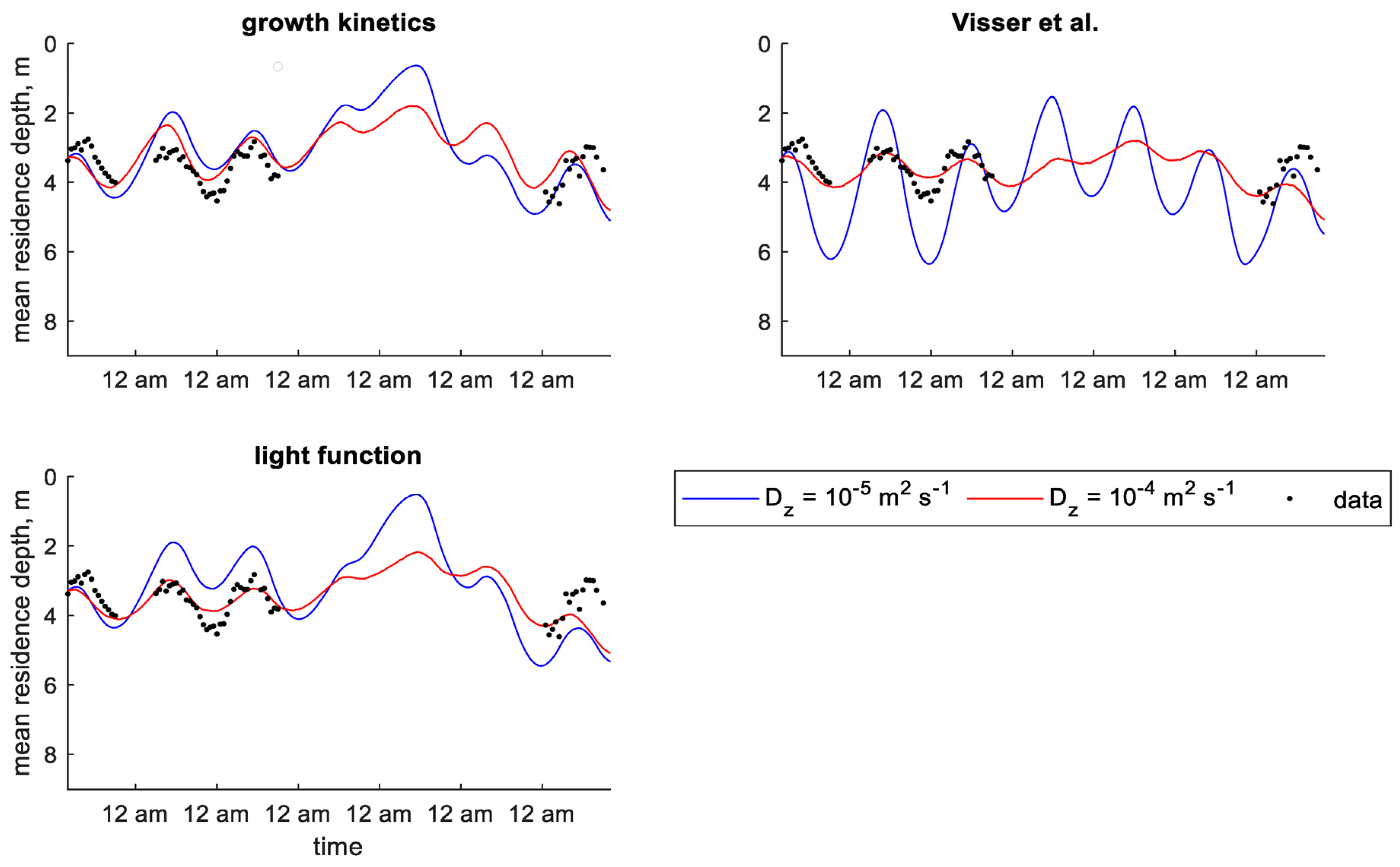
In scenarios using a $D_z$ value of 10⁻⁴ m² s⁻¹, there was not a clear distinction between the predefined and dynamic velocity models. The highest errors resulted from the growth kinetics and light function models without time decay (Table 6). Visually, the predefined velocity models seem to capture the shape of the MRD sinusoidal curve, but the dynamic velocity models predict the average depth more accurately (Figures S17 and S18 in Supplementary Materials). The dynamic models show more daily variation in depth of maximum chlorophyll a concentration for both scenarios but only the growth kinetics and light function models with time decay approximate the correct depth on the second day (Figure 7 and Figure S19 in Supplementary Materials).

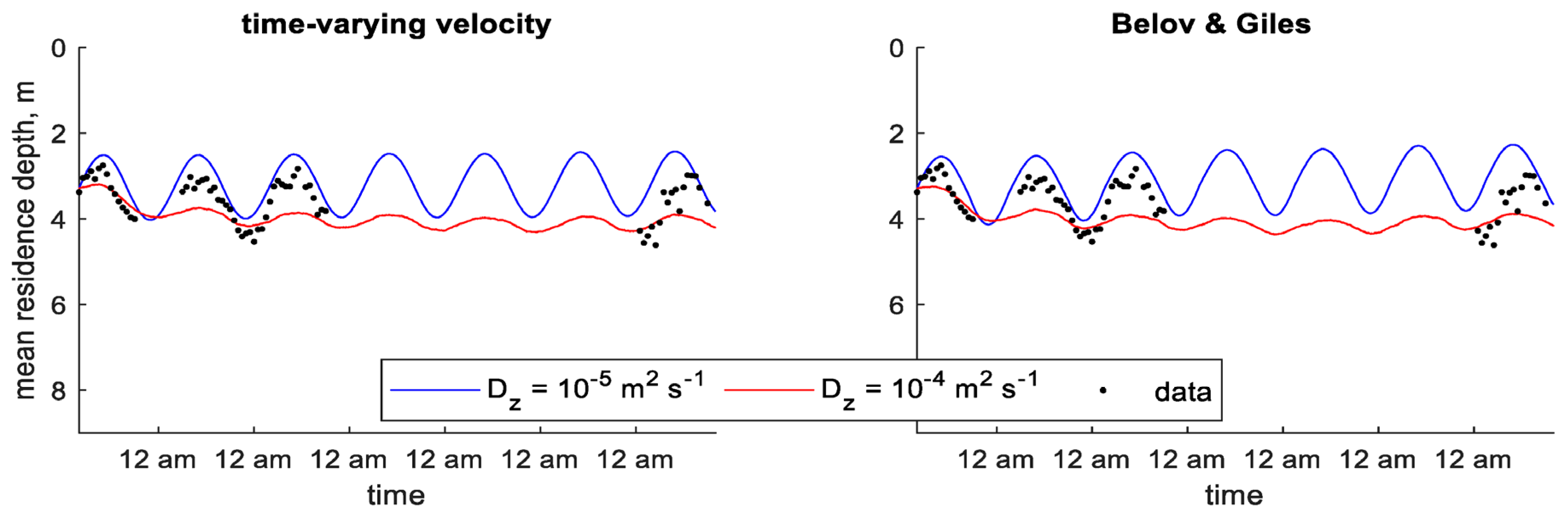
Within the particle-tracking framework, the predefined velocity models gave the lowest error statistics when using the lower value of $D_z$, although the growth kinetics model predicted MRD relatively well (Table 6). Plots of MRD show these models reproducing the general pattern seen in the data throughout the study period (Figure 8). Dynamic velocity models over-predicted MRD amplitude or under-predicted MRD depth (Figure 9). The predefined velocity models in the particle-tracking framework also reproduced the general pattern of depth of maximum chlorophyll a concentration (Figure S23 in Supplementary Materials), which was often over-predicted by the dynamic velocity models (Figure S24 in Supplementary Materials).

In the higher diffusion scenario, the dynamic velocity models resulted in better error statistics than the predefined velocity models for MRD (Table 6). Plots show that these models reproduced the general pattern of MRD, while the predefined velocity models under-predicted MRD amplitude (Figure 8 and Figure 9). While the error statistics show better results for depth of maximum chlorophyll a concentration in predefined velocity models, inspection of the plots suggests that the dynamic velocity models actually perform better in this scenario. The predefined velocity models predict a depth of maximum chlorophyll a concentration that oscillates up and down at a high frequency in the evening, while the dynamic velocity models seem to better reproduce the pattern seen in the data (Figures S23 and S24 in Supplementary Materials).

Similar to the Shennong Stream models, dynamic velocity models applied to the Xiangxi Bay study resulted in better MRD error statistics in the particle-tracking framework compared to the continuum framework for the lower diffusion scenario. In the continuum framework, AMEs ranged from 1.20 m to 1.65 m, while in the particle-tracking framework they were between 0.59 m and 1.00 m (Table 6). The opposite was true for predefined velocity models, which resulted in MRD AMEs of 0.35 m and 0.38 m in the continuum framework and 0.51 m and 0.58 m in the particle-tracking framework. Dynamic velocity models predicted depth of maximum chlorophyll a concentration better in the continuum framework than in the particle-tracking framework, with AMEs of 0.64–0.88 m versus 1.60–2.80 m. Little change was seen between frameworks for predefined velocity models in depth of maximum chlorophyll a concentration.

There was less of a distinct difference between continuum and particle-tracking frameworks in predictions of MRD for the higher diffusion scenario in Xiangxi Bay. AMEs did not change in predefined velocity models and were similar for dynamic velocity models (Table 6). Errors were higher for depth of maximum chlorophyll a concentration in both predefined and dynamic velocity models in the particle-tracking framework compared to the continuum framework.

4. Discussion

Typically, predefined velocity models performed better than dynamic velocity models at lower values of $D_z$. At higher values, predefined velocity models under-predicted concentrations. This is likely due to all particles or model grid cells having the same velocity direction at the same time. The dynamic velocity models in the continuum framework generally made better predictions at higher values of $D_z$. In these models, there is a region below the water surface where downward velocities meet upward velocities. With less diffusion, a high concentration peak tends to develop in these areas. More diffusion spreads out this high concentration; however, these models often under-predicted the depth of cyanobacteria excursion. It is not surprising that predefined velocity models in particle-tracking and continuum frameworks had similar results, since the migration velocity is the same in both frameworks. The biggest difference was that concentrations in the continuum framework became more spatially uniform from diffusion compared to the particle-tracking framework.

In models using dynamic velocity equations, predicted migration timing and depth varied between the two frameworks. A particle-tracking framework is better suited for dynamic velocity models, since these are based on tracking a specific colony though time and space as its density changes. This is not possible in a continuum framework, but the approximation made by solving for density in time and space was able to reproduce the expected pattern seen in field data. The addition of a time decay term generally improved model results in these cases. Predictions of MRD by dynamic velocity models were generally better in the particle-tracking framework than in continuum framework, while predictions of chlorophyll a concentration or depth of maximum chlorophyll a concentration were better in the continuum framework. This suggests that the particle-tracking framework better captures the overall shape of the concentration distribution when dynamic velocity equations are used. However, predictions of concentration at a specific depth are more erroneous. This could be due to many factors including the assumption of no vertical water velocities.

One potential shortcoming of the models presented here is that cyanobacteria density change and movement were assumed to only be dependent on light intensity. Nutrients in the waterbody also play a role in density change [5]. Additionally, turbulence and vertical water velocities can influence vertical migration in cyanobacteria [16].

Particles representing cyanobacteria colonies were assumed to be spherical and to have constant volume, and particle-particle interactions were not considered. In reality, some cyanobacteria species form colonies or filaments that grow over time and do not remain spherical. Velocity of these colonies can deviate from the velocity predicted by Stokes’ law for a sphere due to irregular shapes [59]. Cyanobacteria that has formed a surface scum would also not fit the assumptions of a spherical particle if colonies are stuck together in a mat formation.

Some of the error in the model predictions could also be due to the assumption that the measured chlorophyll a concentration was entirely due to cyanobacteria. While Microcystis species were responsible for the majority of the phytoplankton concentration in both studies, other forms of non-migrating phytoplankton were present. The assumption that chlorophyll a concentration was only due to cyanobacteria could be addressed by modeling all algal species or using a correction factor that accounts for the chlorophyll a contributed by other species. This would require comparison of species analysis to chlorophyll a concentration, such as was reported by Wang et al. [49] and Cui et al. [12], and incorporation of other algae groups.

In the Shennong Stream open water site, field data show MRD continuing to move downward from 04:00 p.m. until sampling stopped at 06:00 a.m., while the models predict it beginning to move upward just after midnight. The pattern seen in the data is unusual compared to data from the Shennong Stream enclosure site as well as Xiangxi Bay, where the MRD consistently begins to move upward around midnight. It is possible that the continued downward trajectory seen in the Shennong Stream open water data was caused by a hydrodynamic event and not cyanobacterial buoyancy regulation. This could explain why the vertical migration models presented here did not capture it, since vertical water velocity was not included and vertical diffusion was assumed to be constant.

Models from this study could be incorporated into a larger water quality model where model predictions of vertical water velocities and other algal species could be predicted. The time-varying, predefined velocity model and the light function model with time decay are good candidates for this. The predefined velocity model is attractive because it is simple while still being able to reproduce vertical migration patterns seen in field studies. The light function model with a time decay term is attractive because it generally gave reasonable results in applications to field studies. This model is preferable to the model based on Visser et al. [13] because it involves fewer calibration variables and often gave better results. It is preferable to the growth kinetics model because it is not dependent on population growth and decay rates. Separating the rate of density change from these variables gives more freedom in calibrating the vertical migration model. Including the decay term almost always led to better model results than when it was not included.

Results from this study show that aspects of cyanobacteria diurnal vertical migration can be simulated using simple input variables such as solar irradiance. The models presented here serve as a foundation for further study and improvement, or incorporation into larger water quality models. Making advances toward more accurately modeling cyanobacteria movement and behavior will allow for better models of lakes and reservoirs and better predictions of HABs, helping with prevention and management of blooms and making waterbodies safer and cleaner.

5. Conclusions

In this study, we reviewed the existing literature on models of cyanobacteria vertical migration. We developed several new models and adaptations of existing models and tested them using field data from published studies. The models tested here were based on either sinusoidal, diurnal vertical movement or buoyancy change as a result of photosynthesis. Models were applied using both continuum and particle-tracking frameworks.

The models of density change showed more daily variation and often made realistic predictions. However, these models included more variables that could be adjusted for calibration, making them more complicated to implement. The density-change models represent a complex biological system reduced to several equations, so simplifications and assumptions have to be made. These models capture the natural process of vertical migration, but erroneous predictions can result from improper calibration especially if necessary data are lacking. The predefined velocity models based on sinusoidal motion were simple to implement and often gave good results, especially at lower values of vertical diffusion.

In tests on field data, models using both continuum and particle tracking frameworks made accurate predictions even while neglecting vertical water motion. Results were not clearly improved by using the particle-tracking framework for predefined velocity models, and the added complexity of such a framework may not be worthwhile for these types of models. Use of a particle-tracking framework improved results from dynamic velocity models because these models are based on density changes and histories of individual colonies.

References

- Howard, A. Problem Cyanobacterial Blooms: Explanation and Simulation Modelling. Trans. Inst. Br. Geogr. 1994, 19, 213–224. [Google Scholar] [CrossRef]
- Lopez, C.B.; Jewett, E.B.; Dortch, Q.; Walton, B.T.; Hudnell, H.K. Scientific Assessment of Freshwater Harmful Algal Blooms; Interagency Working Group on Harmful Algal Blooms, Hypoxia, and Human Health of the Joint Subcommittee on Ocean Science and Technology: Washington, DC, USA, 2008.
- Visser, P.M.; Ibelings, B.W.; Bormans, M.; Huisman, J. Artificial mixing to control cyanobacterial blooms: A review. Aquat. Ecol. 2016, 50, 423–441. [Google Scholar] [CrossRef] [Green Version]
- Belov, A.P.; Giles, J.D. Dynamical model of buoyant cyanobacteria. Hydrobiologia 1997, 349, 87–97. [Google Scholar] [CrossRef]
- Brookes, J.D.; Ganf, G.G. Variations in the buoyancy response of Microcystis aeruginosa to nitrogen, phosphorus and light. J. Plankton Res. 2001, 23, 1399–1411. [Google Scholar] [CrossRef]
- Ganf, G.G.; Oliver, R.L. Vertical separation of light and available nutrients as a factor causing replacement of green algae by bluegreen algae in the plankton of a stratified lake. J. Ecol. 1982, 70, 829–844. [Google Scholar] [CrossRef]
- Bormans, M.; Sherman, B.S.; Webster, I.T. Is buoyancy regulation in cyanobacteria an adaptation to exploit separation of light and nutrients? Mar. Freshw. Res. 1999, 50, 897–906. [Google Scholar] [CrossRef]
- Kromkamp, J.; Walsby, A.E. A computer model of buoyancy and vertical migration in cyanobacteria. J. Plankton Res. 1990, 12, 161–183. [Google Scholar] [CrossRef]
- Kromkamp, J.C.; Mur, L.R. Buoyant density changes in the cyanobacterium Microcystis aeruginosa due to changes in the cellular carbohydrate content. FEMS Microbiol. Lett. 1984, 25, 105–109. [Google Scholar] [CrossRef]
- Kromkamp, J.; Konopka, A.; Mur, L.R. Buoyancy regulation in light-limited continuous cultures of Microcystis aeruginosa. J. Plankton Res. 1988, 10, 171–183. [Google Scholar] [CrossRef]
- Ibelings, B.W.; Mur, L.R.; Walsby, A.E. Diurnal changes in buoyancy and vertical distribution in populations of Microcystis in two shallow lakes. J. Plankton Res. 1991, 13, 419–436. [Google Scholar] [CrossRef]
- Cui, Y.J.; Liu, D.F.; Zhang, J.; Yang, Z.J.; Khu, S.T.; Ji, D.B.; Song, L.X.; Long, L.H. Diel migration of Microcystis during an algal bloom event in the Three Gorges Reservoir, China. Environ. Earth Sci. 2016, 75, 616. [Google Scholar] [CrossRef]
- Visser, P.M.; Passarge, J.; Mur, L.R. Modelling vertical migration of the cyanobacterium Microcystis. Hydrobiologia 1997, 349, 99–109. [Google Scholar] [CrossRef]
- Wallace, B.B.; Hamilton, D.P. The effect of variations in irradiance on buoyancy regulation in Microcystis aeruginosa. Limnol. Oceanogr. 1999, 44, 273–281. [Google Scholar] [CrossRef] [Green Version]
- Cao, H.S.; Kong, F.X.; Luo, L.C.; Shi, X.L.; Yang, Z.; Zhang, X.F.; Tao, Y. Effects of wind and wind-induced waves on vertical phytoplankton distribution and surface blooms of Microcystis aeruginosa in Lake Taihu. J. Freshw. Ecol. 2006, 21, 231–238. [Google Scholar] [CrossRef]
- Zhao, H.; Zhu, W.; Chen, H.; Zhou, X.; Wang, R.; Li, M. Numerical simulation of the vertical migration of Microcystis (cyanobacteria) colonies based on turbulence drag. J. Limnol. 2017, 76, 190–198. [Google Scholar] [CrossRef] [Green Version]
- Zhu, W.; Feng, G.; Chen, H.; Wang, R.; Tan, Y.; Zhao, H. Modelling the vertical migration of different-sized Microcystis colonies: Coupling turbulent mixing and buoyancy regulation. Environ. Sci. Pollut. Res. 2018, 25, 30339–30347. [Google Scholar] [CrossRef] [PubMed]
- Hudnell, H.K. The state of U.S. freshwater harmful algal blooms assessments, policy and legislation. Toxicon 2010, 55, 1024–1034. [Google Scholar] [CrossRef] [PubMed]
- Okada, M.; Aiba, S. Simulation of water-bloom in a eutrophic lake: III. Modeling the vertical migration and growth of Microcystis aeruginosa. Water Res. 1983, 17, 883–893. [Google Scholar] [CrossRef]
- Okada, M.; Aiba, S. Simulation of water-bloom in a eutrophic lake—II. Reassessment of buoyancy, gas vacuole and Turgor pressure of Microcystis aeruginosa. Water Res. 1983, 17, 877–882. [Google Scholar] [CrossRef]
- Howard, A.; Irish, A.E.; Reynolds, C.S. A new simulation of cyanobacterial underwater movement (SCUM’96). J. Plankton Res. 1996, 18, 1375–1385. [Google Scholar] [CrossRef] [Green Version]
- Easthope, M.P.; Howard, A. Simulating cyanobacterial growth in a lowland reservoir. Sci. Total Environ. 1999, 241, 17–25. [Google Scholar] [CrossRef]
- Walsby, A.E. Stratification by cyanobacteria in lakes: A dynamic buoyancy model indicates size limitations met by Planktothrix rubescens filaments. New Phytol. 2005, 168, 365–376. [Google Scholar] [CrossRef]
- Chien, Y.C.; Wu, S.C.; Chen, W.C.; Chou, C.C. Model simulation of diurnal vertical migration patterns of different-sized colonies of Microcystis employing a particle trajectory approach. Environ. Eng. Sci. 2013, 30, 179–186. [Google Scholar] [CrossRef] [PubMed] [Green Version]
- Yao, B.; Liu, Q.; Gao, Y.; Cao, Z. Characterizing vertical migration of Microcystis aeruginosa and conditions for algal bloom development based on a light-driven migration model. Ecol. Res. 2017, 32, 961–969. [Google Scholar] [CrossRef] [Green Version]
- Olsen, N.R.B.; Hedger, R.D.; George, D.G. 3D Numerical modeling of Microcystis distribution in a water reservoir. J. Environ. Eng. 2000, 126, 949–953. [Google Scholar] [CrossRef]
- Wallace, B.B.; Hamilton, D.P. Simulation of water-bloom formation in the cyanobacterium Microcystis aeruginosa. J. Plankton Res. 2000, 22, 1127–1138. [Google Scholar] [CrossRef] [Green Version]
- Wallace, B.B.; Bailey, M.C.; Hamilton, D.P. Simulation of vertical position of buoyancy regulating Microcystis aeruginosa in a shallow eutrophic lake. Aquat. Sci. 2000, 62, 320–333. [Google Scholar] [CrossRef]
- Bonnet, M.P.; Poulin, M. Numerical modelling of the planktonic succession in a nutrient-rich reservoir: Environmental and physiological factors leading to Microcystis aeruginosa dominance. Ecol. Model. 2002, 156, 93–112. [Google Scholar] [CrossRef]
- Rabouille, S.; Thébault, J.M.; Salençon, M.J. Simulation of carbon reserve dynamics in Microcystis and its influence on vertical migration with Yoyo model. Comptes Rendus Biol. 2003, 326, 349–361. [Google Scholar] [CrossRef]
- Hedger, R.D.; Olsen, N.R.B.; George, D.G.; Malthus, T.J.; Atkinson, P.M. Modelling spatial distributions of Ceratium hirundnella and Microcystis spp. in a small productive British lake. Hydrobiologia 2004, 528, 217–227. [Google Scholar] [CrossRef]
- Rabouille, S.; Salençon, M. Functional analysis of Microcystis vertical migration: A dynamic model as a prospecting tool. II. Influence of mixing, thermal stratification and colony diameter on biomass production. Aquat. Microb. Ecol. 2005, 39, 281–292. [Google Scholar] [CrossRef]
- Rabouille, S.; Salençon, M.J.; Thébault, J.M. Functional analysis of Microcystis vertical migration: A dynamic model as a prospecting tool. Ecol. Model. 2005, 188, 386–403. [Google Scholar] [CrossRef]
- Guven, B.; Howard, A. Modelling the growth and movement of cyanobacteria in river systems. Sci. Total Environ. 2006, 368, 898–908. [Google Scholar] [CrossRef] [PubMed]
- Chen, Y.; Qian, X.; Zhang, Y. Modelling turbulent dispersion of buoyancy regulating cyanobacteria in wind-driven currents. In Proceedings of the 2009 3rd International Conference on Bioinformatics and Biomedical Engineering, Beijing, China, 11–13 June 2009; pp. 1–4. [Google Scholar]
- Aparicio Medrano, E.; Uittenbogaard, R.E.; Dionisio Pires, L.M.; van de Wiel, B.J.H.; Clercx, H.J.H. Coupling hydrodynamics and buoyancy regulation in Microcystis aeruginosa for its vertical distribution in lakes. Ecol. Model. 2013, 248, 41–56. [Google Scholar] [CrossRef]
- Ndong, M.; Bird, D.; Nguyen Quang, T.; Kahawita, R.; Hamilton, D.; de Boutray, M.L.; Prévost, M.; Dorner, S. A novel Eulerian approach for modelling cyanobacteria movement: Thin layer formation and recurrent risk to drinking water intakes. Water Res. 2017, 127, 191–203. [Google Scholar] [CrossRef] [PubMed]
- Wang, C.; Feng, T.; Wang, P.; Hou, J.; Qian, J. Understanding the transport feature of bloom-forming Microcystis in a large shallow lake: A new combined hydrodynamic and spatially explicit agent-based modelling approach. Ecol. Model. 2017, 343, 25–38. [Google Scholar] [CrossRef]
- Serizawa, H.; Amemiya, T.; Rossberg, A.G.; Itoh, K. Computer simulations of seasonal outbreak and diurnal vertical migration of cyanobacteria. Limnology 2008, 9, 185–194. [Google Scholar] [CrossRef]
- Trolle, D.; Hamilton, D.P.; Hipsey, M.R.; Bolding, K.; Bruggeman, J.; Mooij, W.M.; Janse, J.H.; Nielsen, A.; Jeppesen, E.; Elliott, J.A.; et al. A community-based framework for aquatic ecosystem models. Hydrobiologia 2012, 683, 25–34. [Google Scholar] [CrossRef]
- Mooij, W.M.; Trolle, D.; Jeppesen, E.; Arhonditsis, G.; Belolipetsky, P.V.; Chitamwebwa, D.B.R.; Degermendzhy, A.G.; DeAngelis, D.L.; De Senerpont Domis, L.N.; Downing, A.S.; et al. Challenges and opportunities for integrating lake ecosystem modelling approaches. Aquat. Ecol. 2010, 44, 633–667. [Google Scholar] [CrossRef] [Green Version]
- Reynolds, C.S.; Irish, A.E.; Elliott, J.A. The ecological basis for simulating phytoplankton responses to environmental change (PROTECH). Ecol. Model. 2001, 140, 271–291. [Google Scholar] [CrossRef]
- Hipsey, M.R.; Antenucci, J.P.; Romero, J.R.; Hamilton, D. Computational Aquatic Ecosystem Dynamics Model: CAEDYM v3; Centre for Water Research, University of Western Australia: Perth, Australia, 2007. [Google Scholar]
- Chung, S.W.; Imberger, J.; Hipsey, M.R.; Lee, H.S. The influence of physical and physiological processes on the spatial heterogeneity of a Microcystis bloom in a stratified reservoir. Ecol. Model. 2014, 289, 133–149. [Google Scholar] [CrossRef]
- Mascarenhas, F.C.B.; Trento, A.E. Particle-tracking method applied to transport problems in water bodies. WIT Trans. Ecol. Environ. 2006, 99, 503–513. [Google Scholar] [CrossRef]
- Chapra, S.C. Surface Water-Quality Modeling; Waveland Press: Long Grove, IL, USA, 2008. [Google Scholar]
- Tennessee Valley Authority. Heat and Mass Transfer between a Water Surface and the Atmosphere; Water Resources Report 0-6803; Lab Report #14; Division of Water Control Planning, Engineering Laboratory: Norris, TN, USA, 1972.
- Jacovides, C.P.; Timvios, F.S.; Papaioannou, G.; Asimakopoulos, D.N.; Theofilou, C.M. Ratio of PAR to broadband solar radiation measured in Cyprus. Agric. For. Meteorol. 2004, 121, 135–140. [Google Scholar] [CrossRef]
- Wang, L.; Cai, Q.; Zhang, M.; Xu, Y.; Kong, L.; Tan, L. Vertical distribution patterns of phytoplankton in summer Microcystis bloom period of Xiangxi Bay, Three Gorges Reservoir, China. Fresenius Environ. Bull. 2011, 20, 553–560. [Google Scholar]
- Reynolds, C.S. The Ecology of Freshwater Phytoplankton; Cambridge University Press: Cambridge, UK, 1984. [Google Scholar]
- Reynolds, C.S.; Oliver, R.L.; Walsby, A.E. Cyanobacterial dominance: The role of buoyancy regulation in dynamic lake environments. N. Z. J. Mar. Freshw. Res. 1987, 21, 379–390. [Google Scholar] [CrossRef]
- Nakamura, T.; Adachi, Y.; Suzuki, M. Flotation and sedimentation of a single Microcystis floc collected from surface bloom. Water Res. 1993, 27, 979–983. [Google Scholar] [CrossRef]
- Long, B.M.; Jones, G.J.; Orr, P.T. Cellular microcystin content in N-limited Microcystis aeruginosa can be predicted from growth rate. Appl. Environ. Microbiol. 2001, 67, 278–283. [Google Scholar] [CrossRef] [Green Version]
- Wu, Z.; Song, L. Physiological comparison between colonial and unicellular forms of Microcystis aeruginosa Kütz (cyanobacteria). Phycologia 2008, 47, 98–104. [Google Scholar] [CrossRef]
- Wu, Z.; Shi, J.; Li, R. Comparative studies on photosynthesis and phosphate metabolism of Cylindrospermopsis raciborskii with Microcystis aeruginosa and Aphanizomenon flos-aquae. Harmful Algae 2009, 8, 910–915. [Google Scholar] [CrossRef]
- Zhang, M.; Shi, X.; Yu, Y.; Kong, F. The acclimative changes in photochemistry after colony formation of the cyanobacteria Microcystis aeruginosa 1: Photoadaptive changes of M. Aeruginosa. J. Phycol. 2011, 47, 524–532. [Google Scholar] [CrossRef]
- Zhu, W.; Li, M.; Luo, Y.; Dai, X.; Guo, L.; Xiao, M.; Huang, J.; Tan, X. Vertical distribution of Microcystis colony size in Lake Taihu: Its role in algal blooms. J. Great Lakes Res. 2014, 40, 949–955. [Google Scholar] [CrossRef] [Green Version]
- Rowe, M.D.; Anderson, E.J.; Wynne, T.T.; Stumpf, R.P.; Fanslow, D.L.; Kijanka, K.; Vanderploeg, H.A.; Strickler, J.R.; Davis, T.W. Vertical distribution of buoyant Microcystis blooms in a Lagrangian particle tracking model for short-term forecasts in Lake Erie. J. Geophys. Res. Oceans 2016, 121, 5296–5314. [Google Scholar] [CrossRef]
- Reynolds, C.S. The Ecology of Phytoplankton; Cambridge University Press: Cambridge, UK, 2006. [Google Scholar]
Figure 1.
Layout of model grid used in cyanobacteria vertical migration models.
Figure 2.
Chlorophyll a concentration profiles measured in Shennong Stream enclosure and open water sites; data extracted from Cui et al. [12].
Figure 3.
Mean residence depth (MRD) calculated from chlorophyll a profiles measured in Shennong Stream open water and enclosure sites; data extracted from Cui et al. [12].
Figure 4.
Mean residence depth and depth of maximum chlorophyll a calculated from chlorophyll a measurements taken in Xiangxi Bay; data extracted from Wang et al. [49].
Figure 5.
Time series of observed and predicted mean residence depth of chlorophyll a concentration in the Shennong Stream enclosure site using predefined velocity models (continuum) [4].
Figure 6.
Time series of observed and predicted mean residence depth of chlorophyll a concentration in the Shennong Stream open water site using dynamic velocity models (particle-tracking) [13].
Figure 7.
Time series of observed and predicted depth of maximum chlorophyll a concentration in Xiangxi Bay using dynamic velocity models (continuum) [13].
Figure 8.
Time series of observed and predicted mean residence depth of chlorophyll a concentration in Xiangxi Bay using predefined velocity models (particle-tracking) [4].
Figure 9.
Time series of observed and predicted mean residence depth of chlorophyll a concentration in Xiangxi Bay using dynamic velocity models (particle-tracking) [13].