
A Laboratory Set-Up for the Analysis of Intermittent Water Supply: First Results


1
Department of Civil and Environmental Engineering, University of Perugia, Via G. Duranti 93, 06125 Perugia, Italy
2
DEWI Srl, Via dei Ceraioli 15, 06134 Colombella, Italy
3
World Bank, Nairobi 00100, Kenya
*
Author to whom correspondence should be addressed.
Water 2022, 14(6), 936; https://doi.org/10.3390/w14060936
Submission received: 17 February 2022
/
Revised: 12 March 2022
/
Accepted: 14 March 2022
/
Published: 17 March 2022
(This article belongs to the Special Issue Intermittent Water Supply)
Abstract
:The evaluation of the impact of intermittent water supply on water distribution systems is a complex task. Laboratory tests, in controlled conditions with virtually no constraints on instrument and device location, allow the analysis of the effects of single parameters on pressures and flows. Within the framework of a research consultancy commissioned by the World Bank, the test network at the Water Engineering Laboratory of the University of Perugia, Italy, was modified to analyse pipe filling and emptying phenomena. Herein we describe the characteristics of the set-up, the available instruments and data acquisition system, as well as the installed devices (e.g., air release and in- and off-line ball valves). The set-up was also designed to investigate the effects of the air flow on the overbilling of water meters. The results of a preliminary test allow the typical phases of the phenomenon to be analysed, including the filling of the pipe with water and the discharging of air, the arrival of the water front at the downstream end causing a pressure variation typical of water hammer, and the emptying process and the filling with air. The analysis allows the operational mechanism to be understood and remedial interventions designed and validated.
1. Introduction
Supply interruption is a common occurrence in water networks, particularly in developing countries. This is a consequence of the demand exceeding the production, causing the reservoirs to run dry. This can have very serious consequences on the structural integrity of the pipes, the quality of the service to the customers, and the accuracy of the customer meters. Interruptions force customers to collect water during times of supply to cover the periods of interruption, modifying the hydraulic operation of the network.
Research in the field of water resources management has mainly considered pipe filling in the context of maintenance purposes, and not the systematic opening and closing of the supply which can result in significant increases of non-revenue water [1,2,3]. Traditionally, the approach to intermittent supply has been to increase production or reduce leakage to enable continuous supply conditions to be achieved. However, it has become clear that this approach is not always cost-effective, leading to the possibility that intermittent supply, though undesirable, will have to be tolerated. As water networks are not designed to withstand the stresses of continuous interruptions to the supply, it means that remedial interventions will be required.
This study has as its objective the definition of technological solutions to mitigate the negative impact of intermittent supply conditions in water distribution systems, within the framework of a research consultancy commissioned by the World Bank to the Department of Civil and Environmental Engineering of the University of Perugia, Italy. The study involved controlled tests in laboratory settings. In this paper, the used set-up and the results of preliminary tests are presented.
After the pioneering work by Martins [4], several papers have evaluated the filling and emptying of single pipes in laboratory tests. Compared with the analysis of the results of tests in complex systems, the filling and emptying of single pipes in laboratories allows the investigation of the basic features of the governing equations and the effects of single parameters in controlled conditions. In the available literature, many experiments deal only with the water filling of systems without considering the air outflow. In view of the objectives of the research, tests with air and water outflow are considered essential to more accurately represent the reality of intermittent functioning conditions in water distribution systems, including the outflow from user connections and leaks as a normal condition.
Following the investigations of Martin and Lee [5,6,7], Zhou et al. [8,9] during experimental tests involving 12 orifice sizes observed three types of pressure-oscillation patterns in a simple short pipe with a downstream orifice. The observed peak maximum pressure values occurred within a fairly consistent orifice size range between 0.171 and 0.254 times the pipe diameter. The sampling frequency of the tests described in the mentioned papers was of 1–2 kHz using pressure transducers having a suitable time response and full scale up to 50 bar were used. The total length of the pipes was shorter than 10 m.
Zhou et al. [10] analysed the expulsion from an end-of-the-pipe orifice in a rapidly filling horizontal pipe, in order to characterise the system transient response. The pipe had a length of 8.8 m and a 40.0 mm inner diameter. It was mostly transparent and made of Poly(methyl methacrylate), PMMA. In the paper, it is shown that the system response, after an initial phase, depended strongly on the orifice size, with small orifices intermittently choked by water and larger orifices leading to large overpressures. Both the initial air volume and inlet pressure influenced the transient response.
A few papers show tests carried out on systems with lengths and diameters larger than 10 m and 50 mm, respectively.
Apolllonio et al. [11] used a laboratory set-up consisting of a PVC-U pipe DN75 with a total length of about 17 m, with an air venting orifice 3.26 m above the downstream valve, to investigate the effects of filling in pipes with ascending and descending profiles.
A large-scale complex experimental setup was used in [12] to investigate the pipe filling and emptying processes. The system had a total length of 275 m and was made of a combination of several pipes with different materials (steel, PVC-U, and PMMA), diameters (DN200 and DN250), and elevations. The pipe filling was achieved by the opening of upstream ball valves according to a defined sequence, with the downstream ball valve open. Emptying was caused by compressed air from an upstream high-pressure tank. Measurements of water levels during the filling allowed the investigation of the air intrusion and entrapping.
In the context of the existing literature, the present laboratory set-up can be considered much more realistic of the real situation thanks to the combination of pipe lengths and diameters and the connection of several off- and in-line valves with different locations and openings.
2. Laboratory Set-Up
The set-up at the Water Engineering Laboratory of the University of Perugia, Italy, was modified specifically for the study.
2.1. The Pipes of the Setu-Up
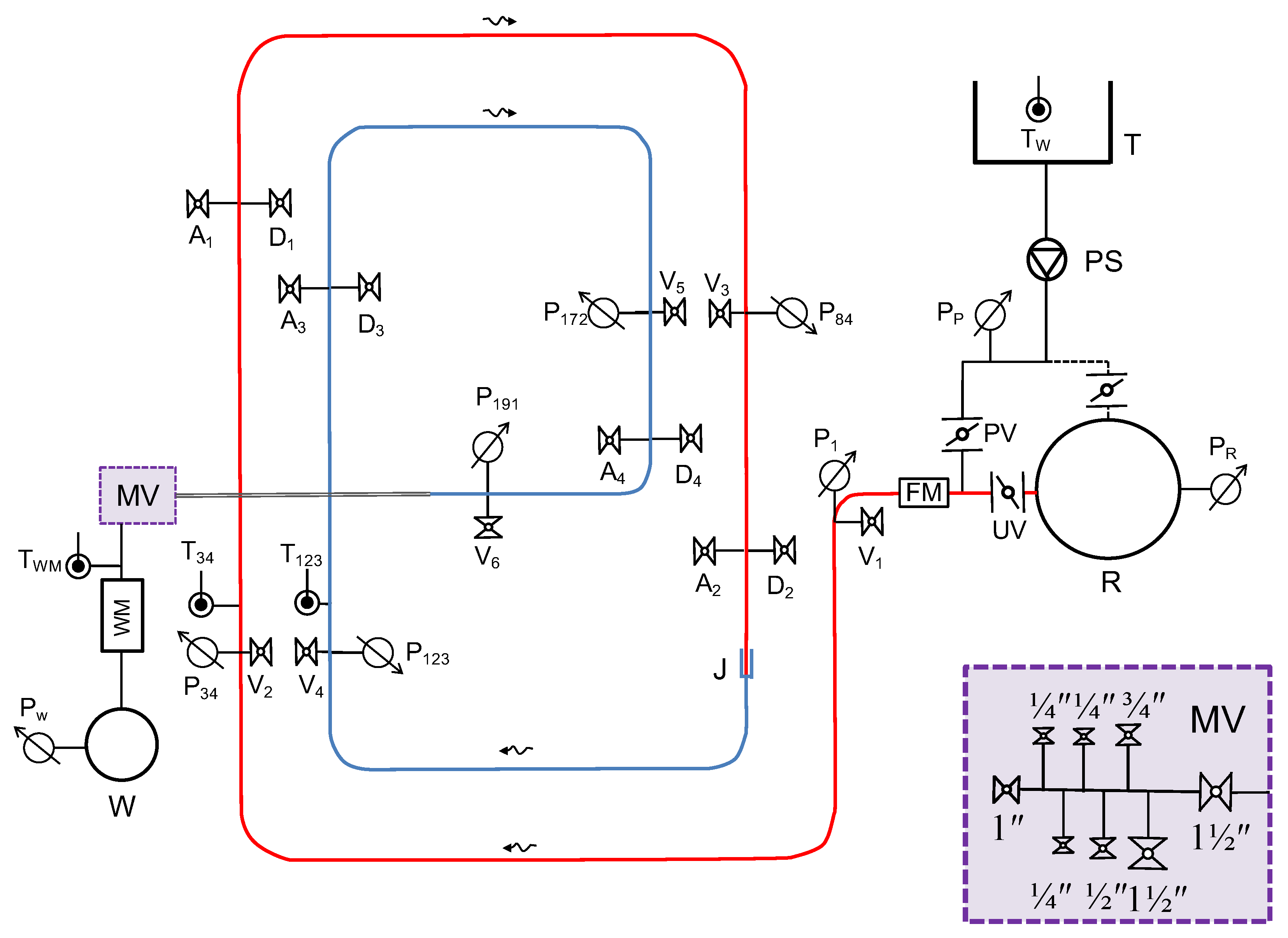
The used experimental set-up consisted of a series of two polymeric pipes (Figure 1), obtained by joining an upstream oriented polyvinyl chloride (PVC-O) DN110 PN16 pipe to a downstream high-density polyethylene (HDPE) DN110 PN10 pipe [13].
The PVC-O upstream pipe had a total length 99.18 m and was made of 6 m sections, each with spigot junctions, with an internal diameter 103.0 mm and a wall thickness 2.7 mm. The HDPE downstream pipe, having an internal diameter 96.8 mm and a wall thickness 6.6 mm, had a total length 92.79 m and was obtained by the sleeve junction of two trunks of about 50 m each. The PVC-O and HDPE pipes had the same external diameter and the joint between them (J in Figure 1) was obtained simply by inserting about 0.17 m of the upstream end of the HDPE pipe in the bell at the downstream end of the PVC-O pipe. The standard PVC-O gasket guaranteed joint tightness.
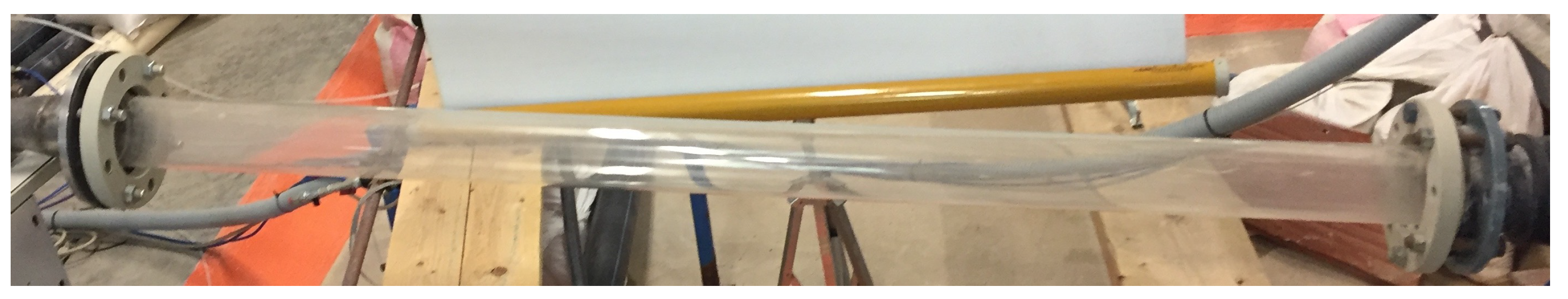
At the end of the HDPE pipe, a PMMA trunk with the same inner diameter of the DN110 HDPE pipe was used to allow the visualisation of the air and water content (Figure 2). The PMMA trunk could be substituted with an HDPE pipe of the same length.
A further length with a 45° bend was also used instead of valves and manifold, to avoid any diameter reduction at the downstream end of the system and to control the water outflow in the laboratory.
The pipes were fixed to the laboratory floor, which has an elevation variation of less than 10 cm from one end to the other. The downstream part of around 6 m length including the PMMA trunk or its HDPE pipe substitute rose up to 110 cm at the downstream valve MV.
2.2. Feeding Conditions
The system was fed by the air vessel R, having a capacity of about 10 m3, which in turn was fed by the pumping system through a manifold. The use of an air vessel instead of a free surface tank allowed large pressure values at the inlet. The tests started from steady-state conditions with the pump switched on, no flow, and the air vessel at a pressure of about 2 bar. The butterfly valve PV remained closed and the pipe was filled by the opening of the butterfly valve UV.
To investigate the effects of different feeding conditions, a by-pass pipe was also used in order to directly connect the manifold of the pumps to the system and by-passing the air vessel. In this case, the valve UV remained closed and the valve PV was open for the whole duration of the test. The pressure transducers PR and PP measured the pressure in the air vessel and on the manifold downstream of the pump PS, respectively.
2.3. Valves: Downstream Valves, Drains, Vents, and Air Valves
Assessment of the effects of the varying downstream valve openings could not be defined accurately and consistently by the valve position alone. A much more precise and objective way of doing so was achieved by the complete opening of valves with different diameters.
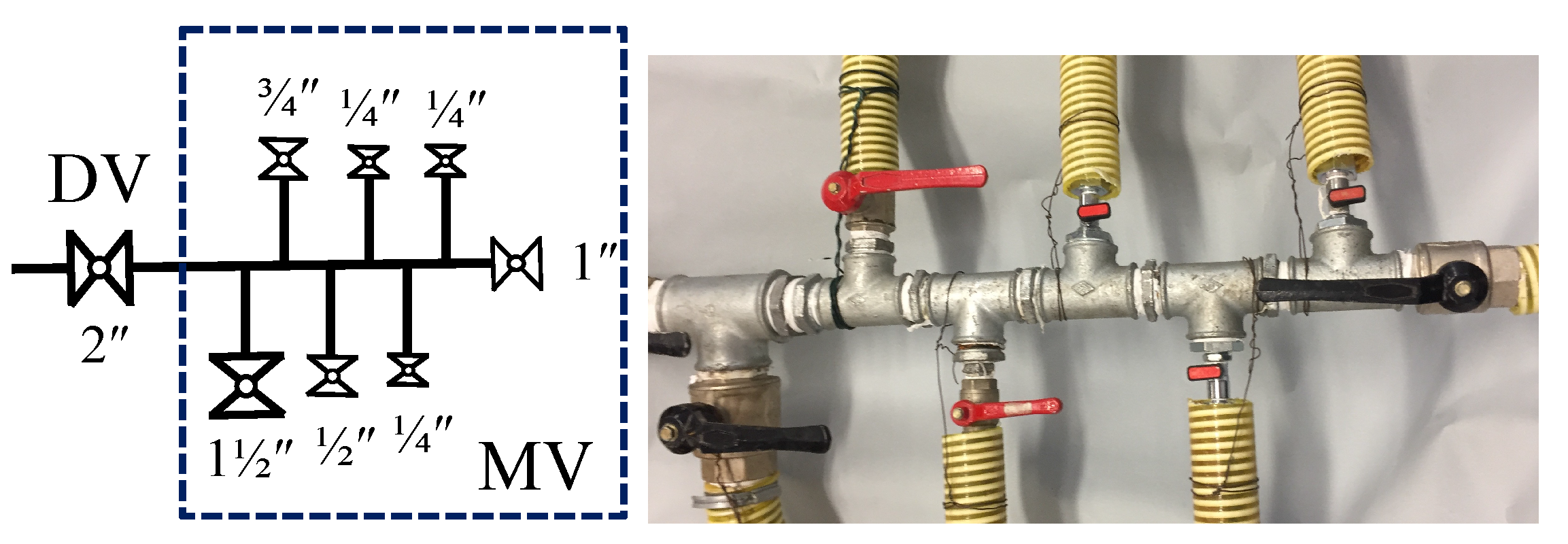
Different devices were connected at the downstream end of the pipe. A small conical trunk or a plate allowed the direct connection of a 2″ valve and, by means of diameter reductions, of other valves with smaller diameters. A valve manifold with multiple valves (MV in Figure 1) was also used, simplifying the switch between different test conditions (Figure 3). Ball valves of 1½″, 1″, 3/4″, 1/2″, and 1/4″ were used.
As mentioned, the no-valve downstream condition was also investigated by removing all the downstream devices (plate or conical trunk and manifold), but in this case an HDPE DN110 trunk with a 45° bend was added to allow the proper water collection.
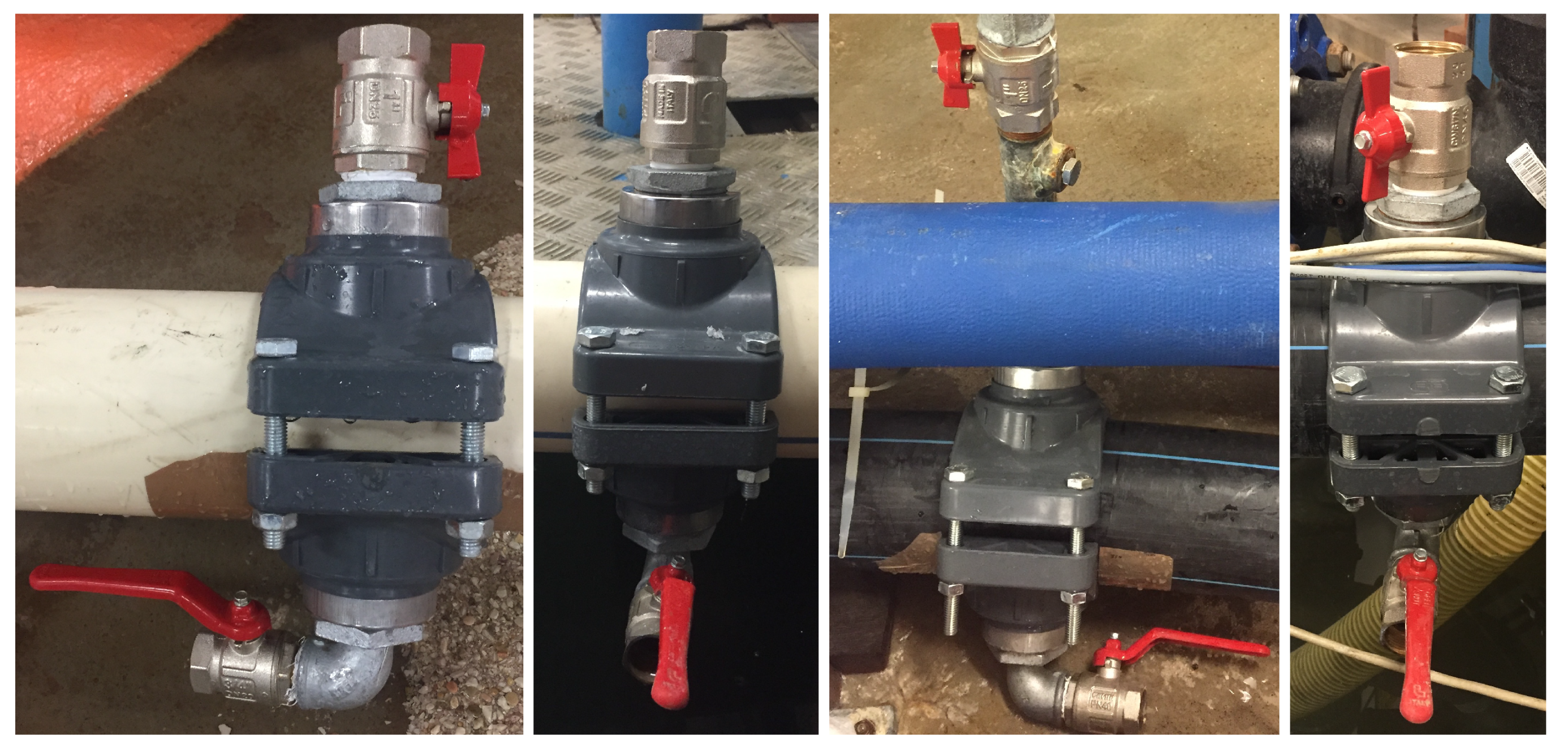
Four drains were introduced to allow the pipe emptying at the end of the tests (Figure 4). Each drain was made of a 3/4″ ball valve connected to the bottom of the pipe. The locations of the drains D1 to D4 are shown in Figure 1. At the same locations, 1″ ball valves were also installed on the top of the pipe (A1–A4 in Figure 1) to be used as vents to speed up the pipe emptying between tests and as connections for the 1″ air release valve.
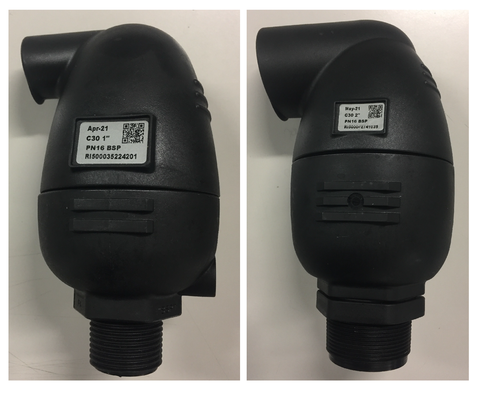
Two air valves were used to evaluate the effects on transients of air valves normally operating in water pipeline systems with the aim of discharging air during the pipe filling and enabling the air ingress during the emptying. The air valves shown in Figure 5 (model C30, produced by Bermad) have different inlet size (1″—DN 25 and 2″—DN50). The 1″ air release valves were connected to valves A1 to A4.
2.4. Water Meter Testing
Two of the most common types of water meters were used for the tests, that is, a protected rollers single-jet water meter and a protected rollers multi-jet water meter. The characteristics of the water meters are given in Table 1.
The water meters were connected to the 3/4″ valve of the manifold MV, with small steel connections placed upstream and downstream as required by regulation and good practice to improve the operating conditions of the meter.
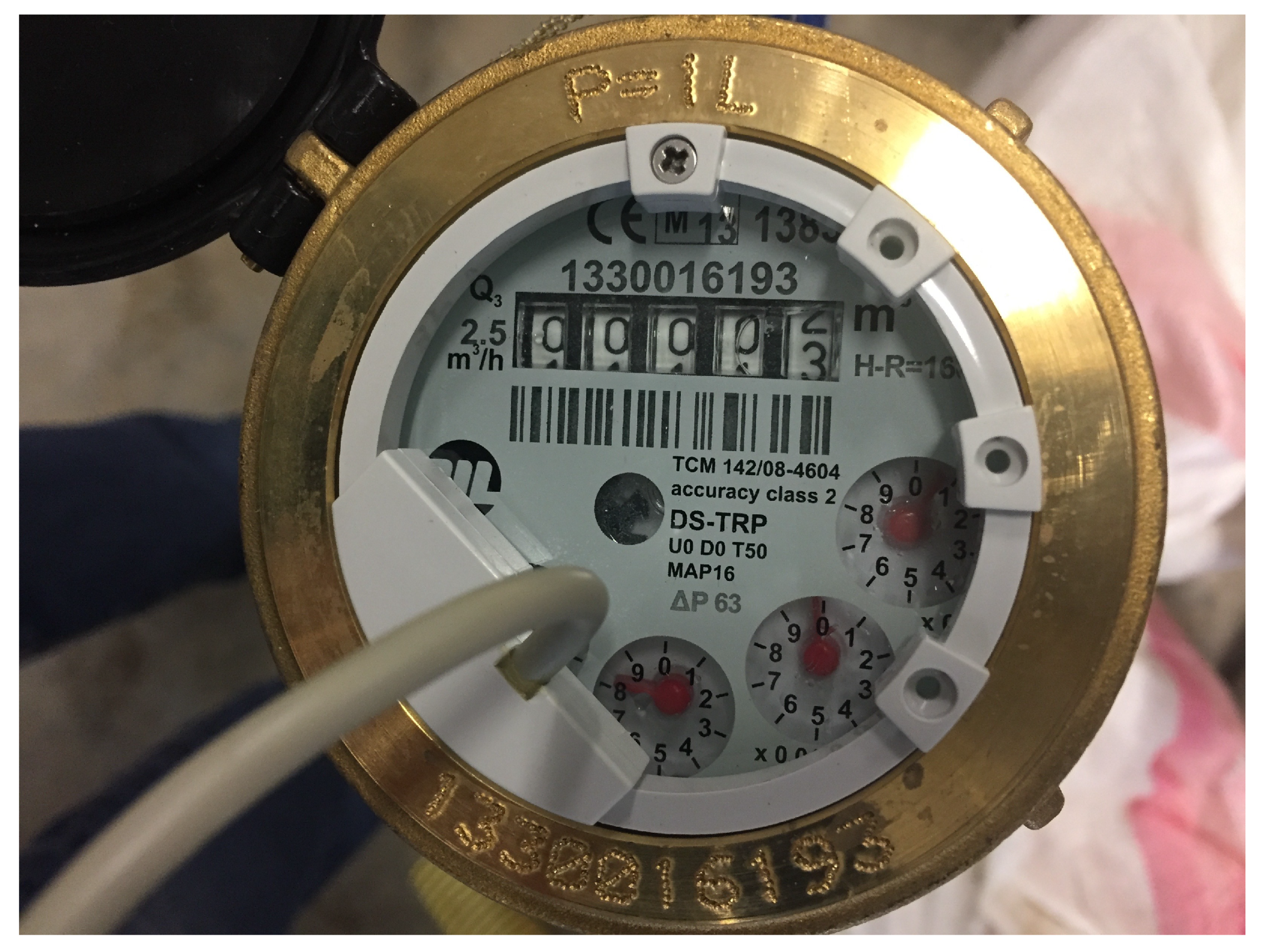
A reed switch pulse unit was connected to the water meters (Figure 6). The pulse unit comprised an electrical switch operated by a magnetic field (reed switch) generated by the rotation of one of the counter hands. Depending on the chosen resolution, the pulse unit transmits up to a pulse per litre to the data acquisition system.
The outlet of the water meter was connected by an HDPE ½″ trunk to the top of a tank (Figure 7) to collect the water outflow. The measurement of the water level in the tank was by the pressure transducer PT, which provided the measure of the water volume which actually passed through the water meter. The tank had a diameter of 630 mm and a height of 1170 mm. The diameter was chosen so that a pressure transducer with a full scale of 1.53 m (150 mbar) and accuracy of 0.1% f.s. was able to measure the volume with an accuracy of less than 0.5 L.
Both the water level in the tank and the pulses generated by the water meter were acquired in time, in order to compare the actual volume of water collected with the water volume measured by the water meter.
3. Instruments
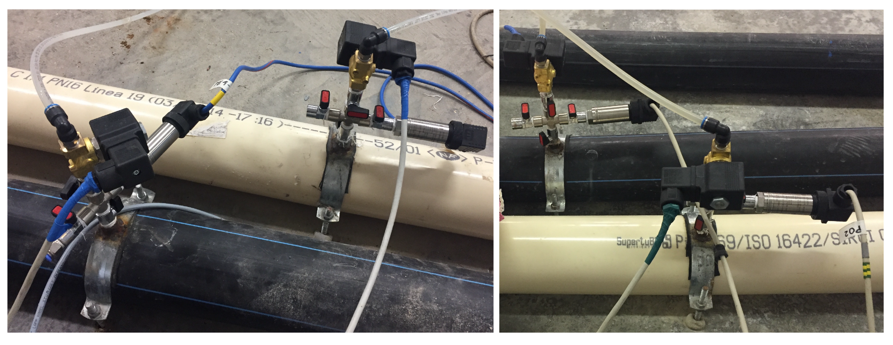
The pressure transducers along the pipe were connected at the measurement sections to the upper part of the pipe by a 1/4″ cross (Figure 8) with a remotely controlled solenoid valve and a ball valve at the other ends.
Different pressure transducers were used during the tests, including TRAFAG ECT 8473 thick-film-on-ceramic pressure transmitters (accuracy of 0.30% of the full scale, f.s.), MEAS M5100 gage pressure transducers (accuracy of 0.25% f.s.), GEMS 2200 gage pressure transducers (accuracy of 0.20% f.s.), and GE UNIK 5000 pressure sensors (accuracy of 0.10% f.s.). Table 2 summarises the location of the pressure transducers during the preliminary test shown in the following sections.
The locations of the pressure transducers (P1, P34, P84, P123, P172, and P191) and solenoid valves (V1 to V6) are shown in Figure 1. The pressure transducers PR, PP, and PT were connected to the air vessel, to the pump manifold, and to the tank, respectively.
An ISOIL electromagnetic flow meter, FM, was used to measure the discharge in steady-state conditions, having an accuracy of 0.2% of the measured value. The meter can measure the mean flow velocity only when the pipe is completely filled with water.
Four Pt100, class 1/10 DIN, resistance thermometers, with an accuracy of 0.15 °C were used during tests to measure the temperature of the water at the input in the air vessel, TR, at the external surface of the HDPE pipe, T123, at the external surface of the PVC-O pipe, T34, and at the water meter, TWM.
The acquisition frequency of the data was set to 1 Hz for the flow meter, 1.25 Hz for the thermometers, and 2048 Hz for the pressure transducers.
4. Data Acquisition System
The data acquisition system used was based on a National Instruments Compact-DAQ NI-9188 chassis, with eight slots for input/output modules, which provided the signal conditioning and analogue-to-digital conversion. Each module contained measurement-specific signal conditioning to isolate the data and filter out noise. Six NI-9218 two-channel modules combined with the NI-9983 adapters were used for universal measurements, which supplied the instruments and acquired the 4–20 mA signals from pressure transducers and electromagnetic flowmeters. An NI-9217 module acquired the temperature from the four PT100 RTD thermometers. A bidirectional digital NI-9401 module with eight digital input/output channels (DIO) counted the pulses coming from the reed contacts of the flow meters.
For the purposes of the research activity, a graphical interface in LabView was specifically developed to acquire the synchronous data from all the C-DAQ modules. In addition to current and temperature data, the flow rate was automatically evaluated by the pulses sent from the water meter pulse unit and was shown in real-time on the monitor.
5. Results of the Preliminary Test
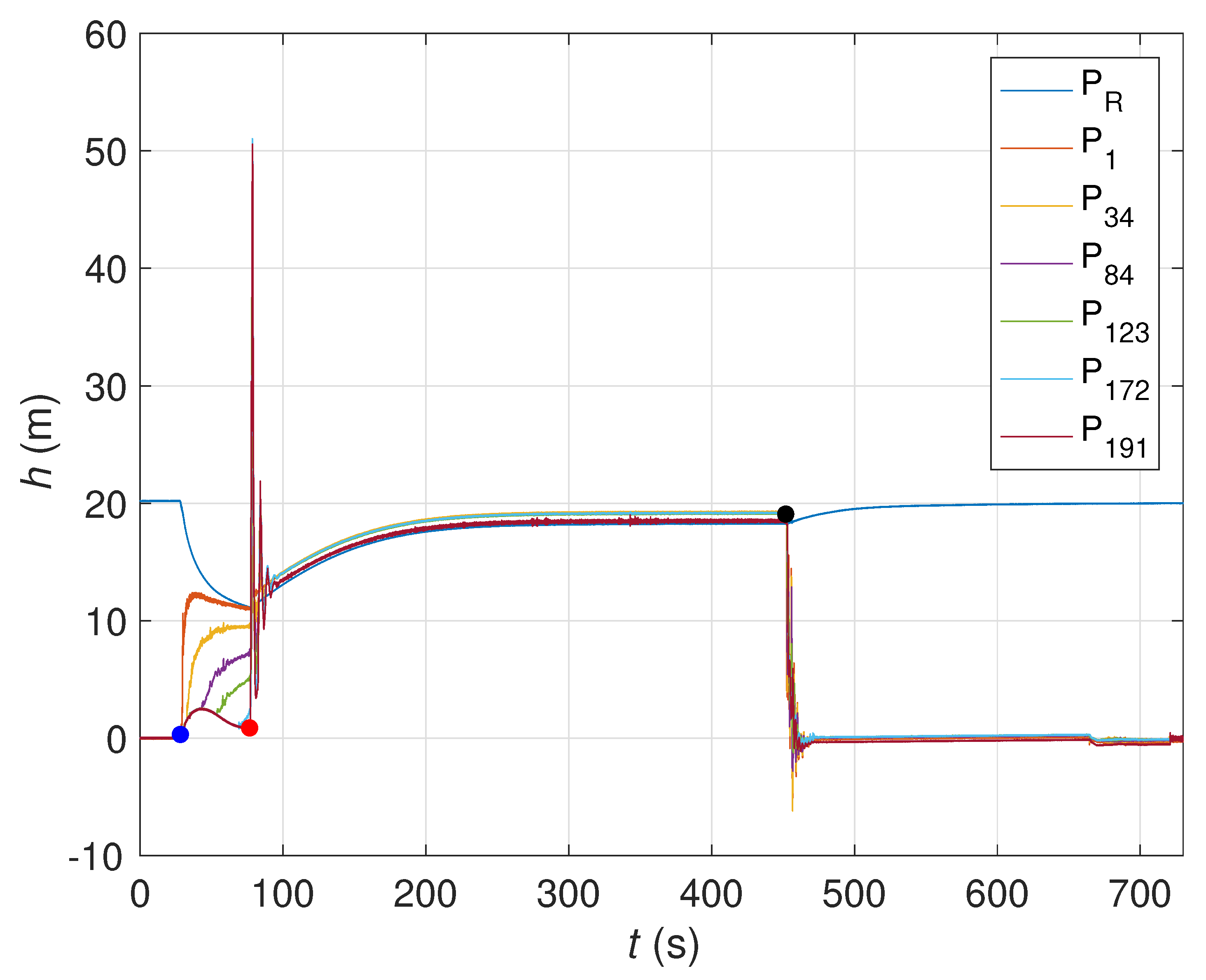
The main characteristics of the filling and emptying processes are described in this section, with reference to the results of a preliminary test. The pressure variations at all the measurement sections during the test are shown in Figure 9.
Both filling and emptying of the pipe were investigated. The former can be divided into the actual filling of the pipe (i.e., in the water front propagation in the pipe), and the water hammer phenomenon that could occur starting from when the water front reaches the end of the pipe. Each test can be divided into four different phases, as detailed below.
In the first phase, the pipe is empty. If the pumping system is connected to the air vessel and not directly to the pump, the air vessel is maintained at a constant pressure, with UV and PV closed. If the system is fed directly by the pump, the initial status is off with UV closed and PV opened. Since the system was fed by the air vessel for the test, in the first phase the pressure at all the measurement sections was zero because the pipe was empty with the exception of the transducer PR connected to the air vessel, where the pressure head was about 20 m (Figure 9).
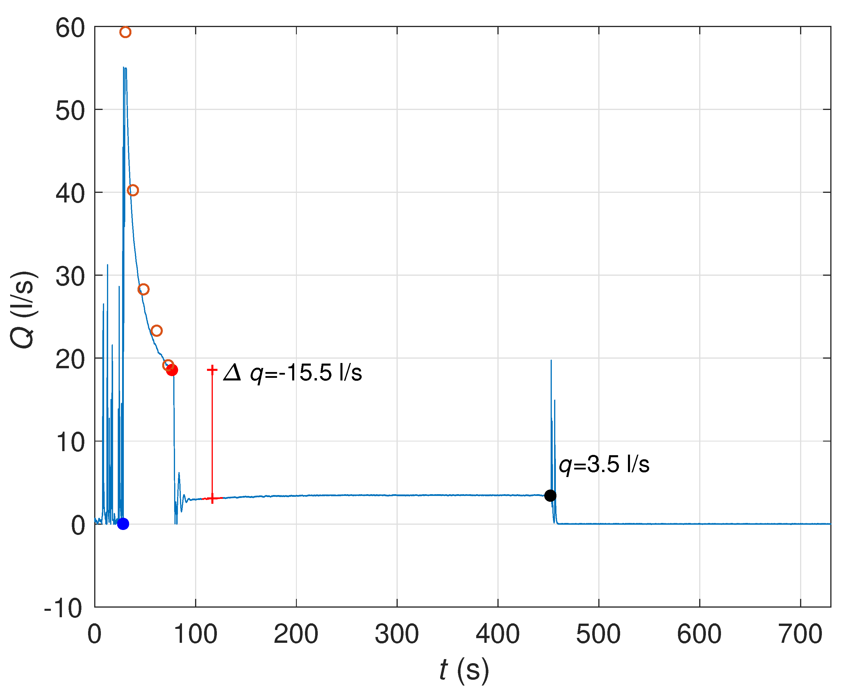
The second phase of the test starts with the filling of the pipe with the opening of UV or the switching on of the pump. In Figure 9, the blue circle denotes the opening of UV in the preliminary test and the start of the pipe filling. The same symbol is also used in Figure 10 where the flow variation in time measured by the flow meter FM during the same test of Figure 9 is shown.
With reference to the electromagnetic flowmeter (FM) and to the shown measurements, it is worth mentioning the following:
- -
- FM does not measure the discharge when the pipe is not full, i.e., before the valve opening and for a period of time after;
- -
- The time response is about 1 s and hence data variations at frequencies higher than 1 Hz are meaningless;
- -
- FM measures only the absolute value of the discharge, i.e., positive values for both forward and backward flows.
The arrival of the water front at the downstream valve (red circle in Figure 9 and Figure 10) can be considered as the end of the filling process and the beginning of the third part, i.e., when the water hammer phenomenon occurs.
The fourth and last part is the emptying of the pipe, which for the considered test corresponded to the closure of the upstream valve UV (black circle in Figure 9) and not by the pump switch off.
The pipe filling, the water hammer, and the emptying phases of the preliminary test are described in more detail in the following sections.
5.1. Pipe Filling
The filling of the pipe started with the opening of the upstream valve UV. The pressure in the air vessel, corresponding to the blue line in Figure 9, was constant before the valve was opened but decreased during this phase of the test. In fact, the water outflow from the air vessel could not be replaced by the feeding pump at the given pressure and, as a consequence, the air vessel started emptying and the pressure decreased.
The water front moving downstream pushed the air in the empty pipe in front of it and the air flowed out of the downstream 1″ open valve.
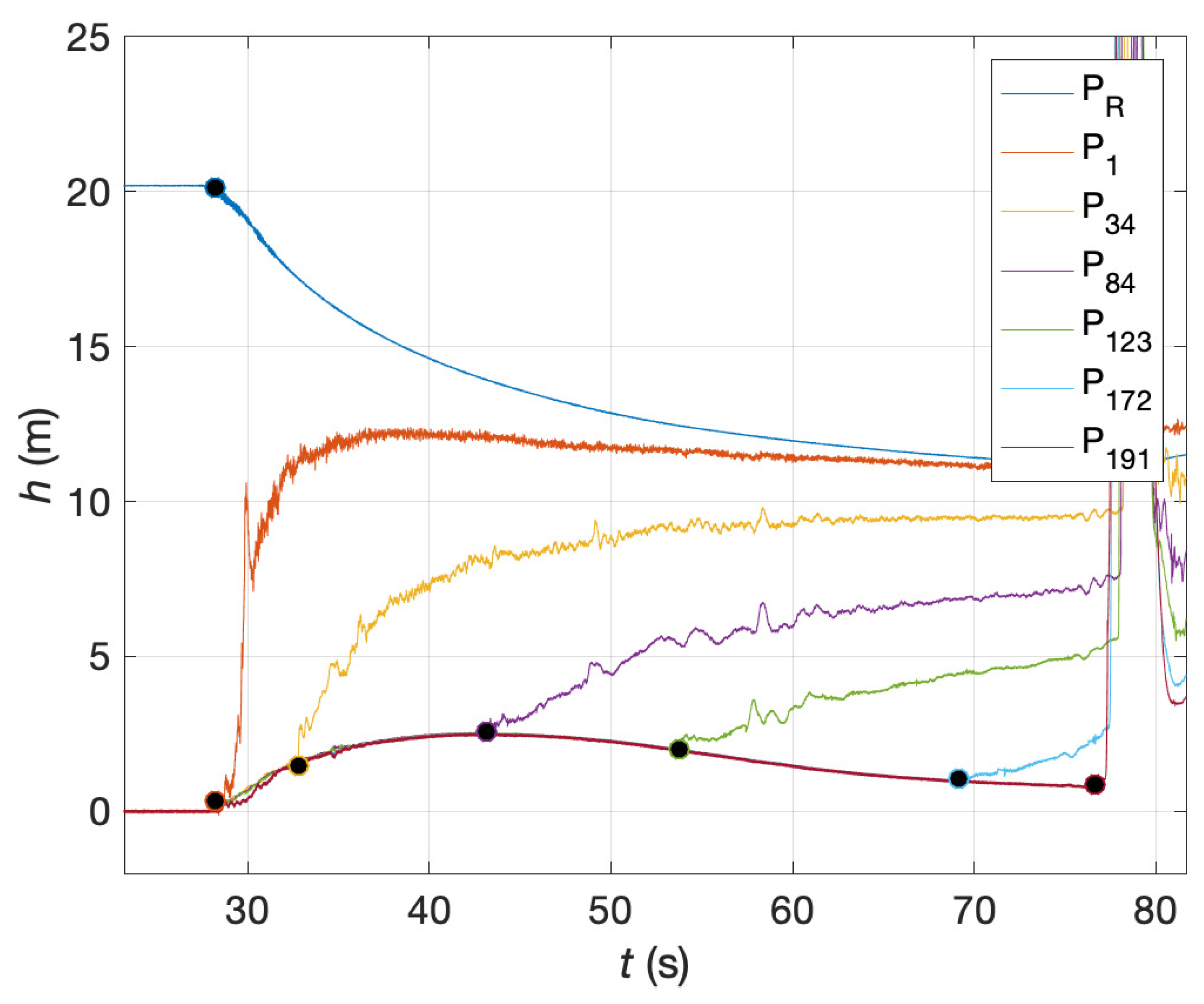
Figure 11 shows in detail the same pressure variations of Figure 9 during the pipe filling. After the opening of UV, the water front almost instantaneously reached the first pressure transducer P1, with a consequential pressure increase (black circle around t = 28 s). Differences between the pressure measured in the air vessel (blue line) upstream of UV and at the pressure transducer P1 (red line) a few meters downstream of the valve UV can be explained by the minor losses at the valve UV. The head loss decreased over time due to the decrease of the discharge passing through the valve (Figure 10).
The pressure measurements at all the other transducers showed the same behaviour: a fairly constant pressure at all the points before suddenly increasing. This can be explained by the fact that initially, the transducers measured the air pressure in the pipe and this pressure did not vary along the pipe, even if the air was moving. Then, when the water front arrived at the measurement sections the pressure transducer started measuring water pressure instead of air pressure.
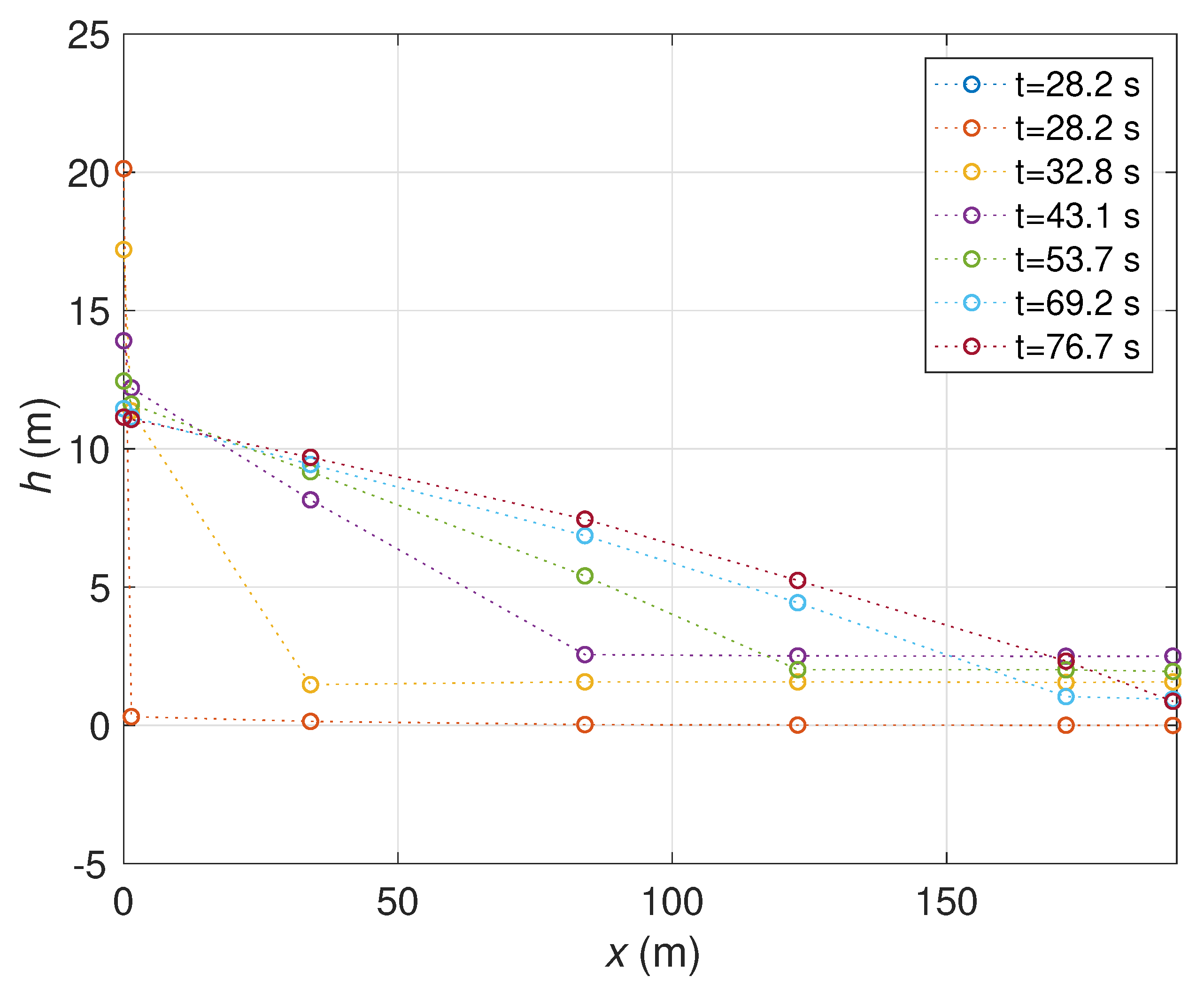
Pressure differences between the transducers were due to the water movement, which caused head losses and a decreasing energy grade line in the downstream direction. The variation in time of the pressure head line is shown in Figure 12. The selected times correspond to the time of arrival of the water front at the pressure transducer. The mean slope decreased over time due to the increase of the downstream air pressure and length of the water-filled pipe, consistently with the decrease of the discharge.
The arrival times of the water front also allowed an estimate to be made of the mean discharge. In fact, it can be assumed that the pipe inner volume between the two measurement sections was filled in the interval between the arrival times at the same sections. The values of the mean discharge between two arrival times (red hollow circles) are compared in Figure 10 with the discharge measured at FM (blue line).
5.2. Water Hammer
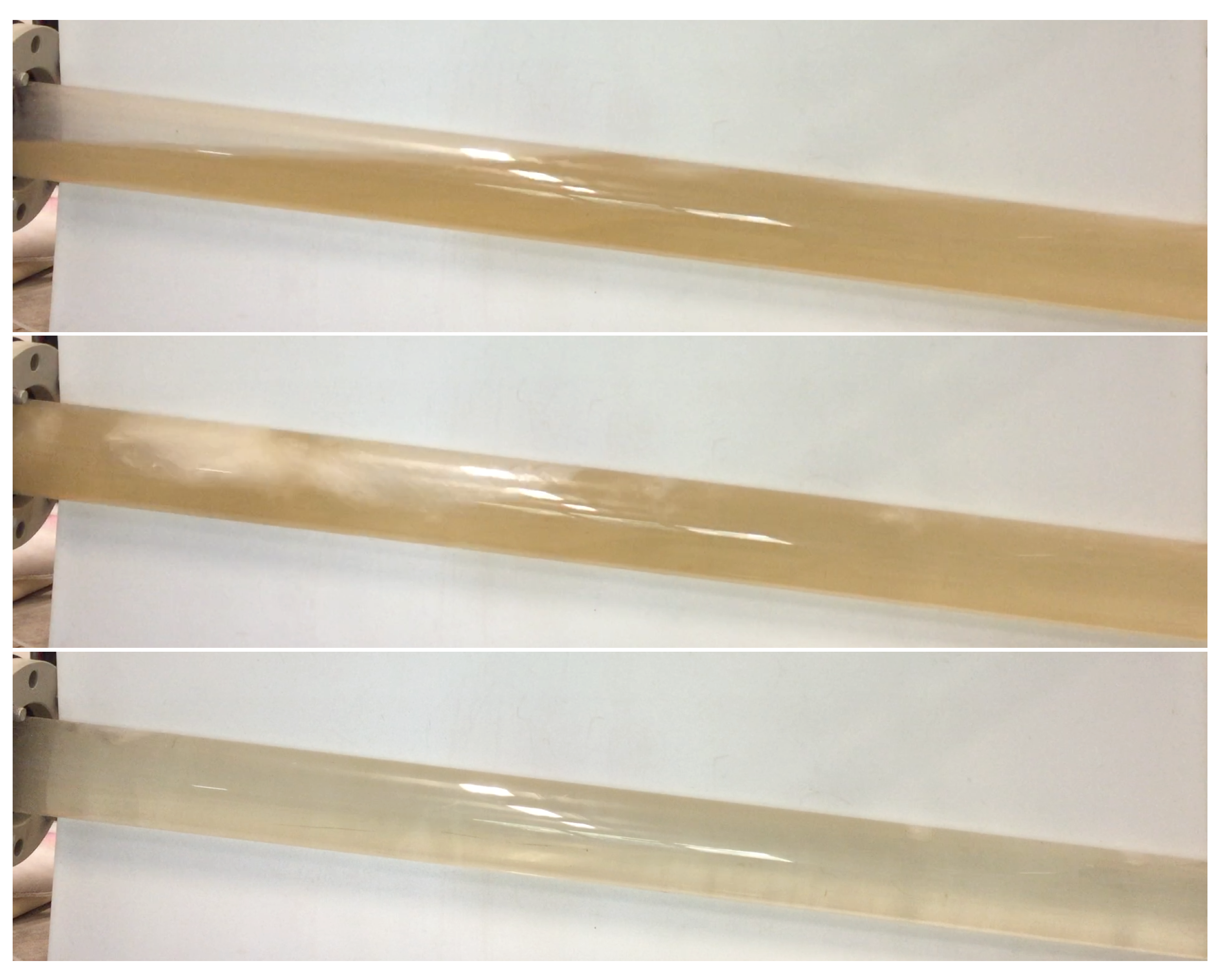
When the water front reached the open downstream 1″ valve (Figure 13), the water started flowing through it instead of air.
Since the volume of air per second passing through the valve before the water front arrival was larger than the water volume per second passing through the same valve after the water front’s arrival, the water front velocity was suddenly reduced. As a consequence, the pressure of the water at the valve increased with a variation proportional to the velocity change.
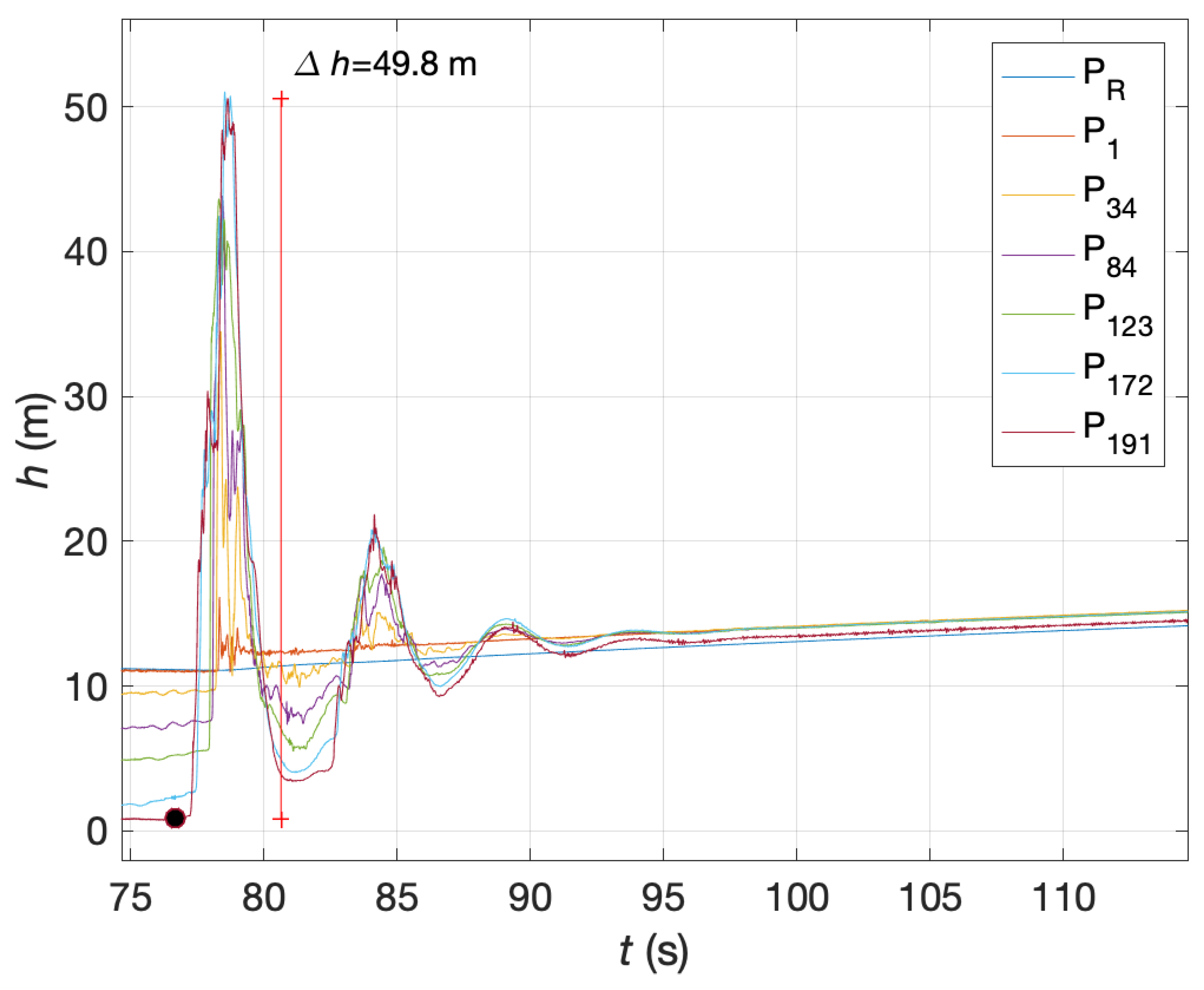
In Figure 14 the same pressure variations of Figure 9 are shown, in a time interval of about 35 s after the water front arrival at the end section. It can be seen that the sudden increase in the pressure at the transducers moved from downstream to upstream (i.e., P191 and then P172, P123, and so on), suggesting that a pressure wave was propagating in the pipe in the upstream direction. Once the pressure reached its maximum it started decreasing from downstream to upstream, suggesting that the pressure wave was reflected by the upstream air vessel and propagated downstream as a negative pressure wave. This behaviour is typical of a water hammer phenomenon caused by the sudden closure of the downstream valve.
The relationship between the velocity decrease and the pressure increase can be investigated by measuring the pressure increase after the water front arrival at the transducer P191 (e.g., 49.8 m in Figure 14) and assuming that the difference in the discharge before and after the water front arrival time can be estimated by the FM measurements (e.g., −15.2 L/s in Figure 10). In this case, the Allievi–Joukowsky formula holds, assuming a value of the wave speed in the pipe of about 250 m/s. Transient tests caused by the downstream valve closure in the system for filled pipes yielded values of the wave speed of more than 300 m/s [13,14,15,16,17] but in this case differences could be due to the air content, which significantly reduced the wave speed.
The pressure oscillation caused by the arrival of the water front at the downstream end section vanished in a few seconds, with the system reaching the steady-state conditions after several minutes. In Figure 9 the water front reached the downstream section at 77 s and the pressure oscillations lasted about 30 s. After the oscillations vanished, the pressure at the measurement sections kept increasing everywhere until the steady-state conditions were reached in about 3 min.
5.3. Pipe Emptying
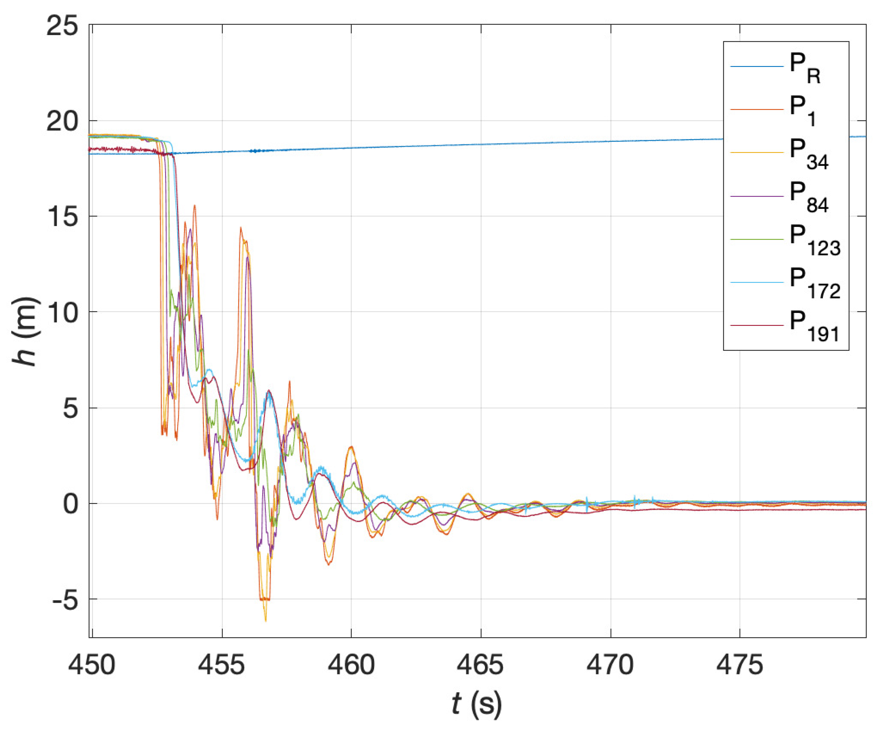
The emptying of the pipe started with the closure of the valve UV around 452 s (Figure 15). The sudden closure of the valve caused a decrease in the pressure at the upstream end of the pipe and then at all the other measurement sections downstream. The following pressure oscillations can be explained by the propagation and reflection of a negative pressure wave caused by the discharge decrease. Whereas the water hammer caused by the arrival of the water front at the downstream valve was characterised by the increase of the pressures at the transducers, the emptying phase was characterised by negative variations, which can cause negative relative pressures inside the pipe. As an example, in Figure 15 negative pressure in the pipe started appearing at 454 s. This situation is particularly dangerous in a functioning water distribution system because negative pressures facilitate the intrusion of polluted water in the pipe through leaks.
Around 20 s after the valve closure, the pressure transducer measurements returned to the initial values. In fact, the instruments were not able to distinguish between the filled pipe with water at atmospheric pressure and empty pipe conditions. In fact, at the end of the emptying phase, the pipes were still filled with water and it took more than 30 min with drains and vents open to almost completely empty the pipe and start with a new test.
6. Water Meter Measurements
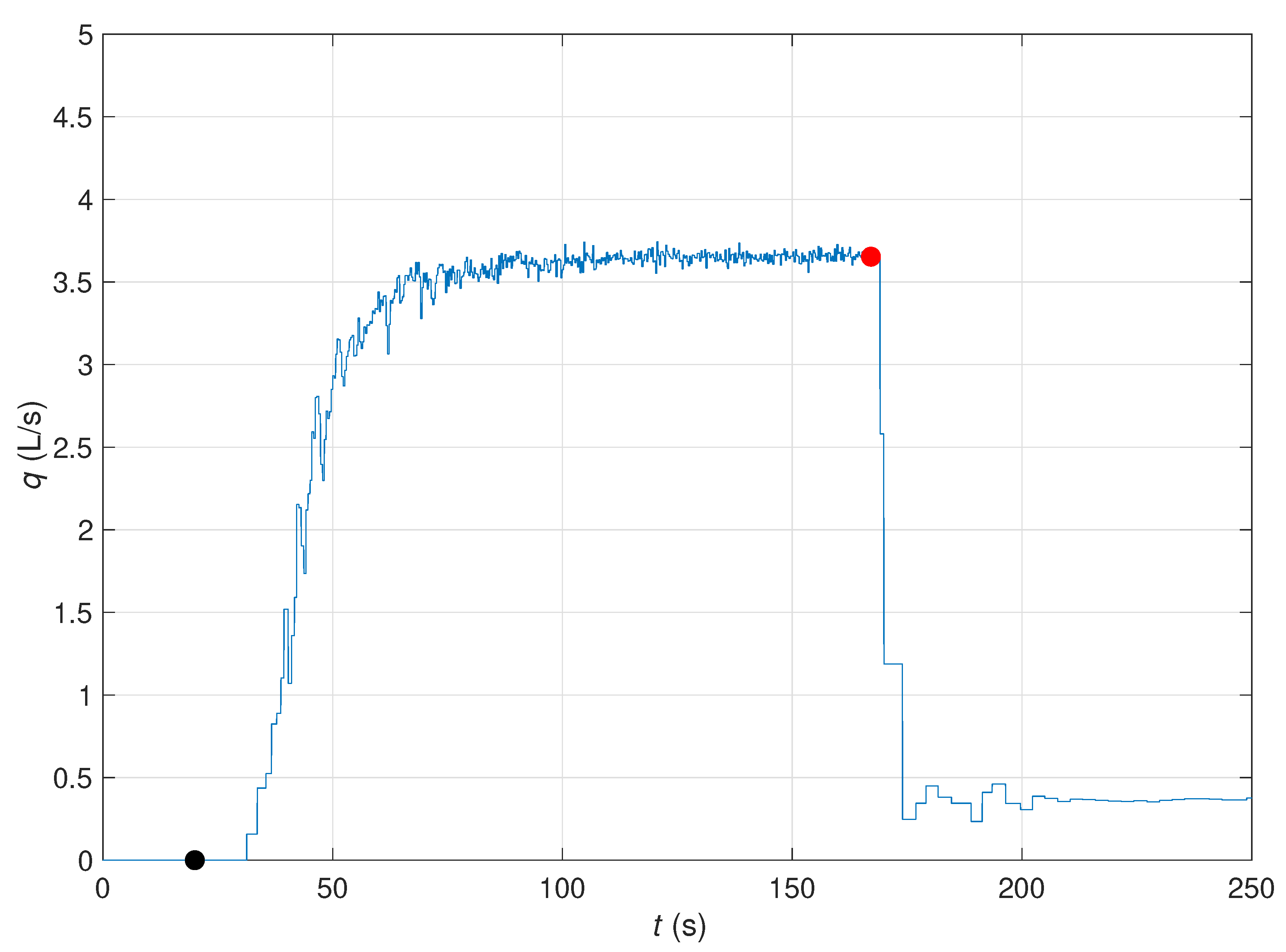
Figure 16 shows the typical measurements obtained by the elaboration of information coming from the water meter pulse unit. Considering that each pulse corresponded to 1 L of water which passed through the water meter, the time lag between two successive pulses could be used to evaluate the mean discharge associated with that time interval. As an example, if the lag time between two pulses was 2 s, a mean discharge value of 0.5 L/s was associated with that interval.
In Figure 16, the black circle denotes the opening of the upstream valve and the beginning of the pipe filling while the red circle denotes the arrival of the water front at the water downstream section. For the illustrated test, the rotation speed of the water meter impellers increased in time due to the air flow and reached a value corresponding to a water discharge of about 3.6 L/s. When the water started flowing through the water meter, the measured discharge suddenly decreased to about 0.4 L/s. These two values must be compared with the water meter Q4, which is the maximum allowed discharge metered value. For the water meter used in the test, it corresponds to Q4 = 0.87 L/s and hence, during the test, the water meter in dry conditions reached an impeller rotation speed four times greater than the maximum allowable. This also means that in the test conditions, the water meter recorded an overbilling of 463 L due to the passage of air.
7. Conclusions
The filling and emptying of pipes in intermittent supply conditions are complex phenomena that can seriously impact the structural integrity and quality of service of water distribution systems, with an increase in the risk of contamination, non-revenue water, and deterioration of infrastructures. Laboratory tests on a simple set-up can simplify the investigation, reducing the number of involved parameters and increasing the density and types of measurements.
In the literature, the results of several tests are shown on “small” set-ups, with lengths of 10 m and diameters of 10 m. Only a few tests involved “large” set-ups with lengths of 10 m and diameters of 10 m. In order to fill the research gap, the “large” set-up available at the Water Engineering Laboratory at the University of Perugia was modified to investigate the effects of valve location, type and opening degree on the filling and emptying. These tests are valuable in evaluating the effects of preventative strategies which can be implemented in the field to reduce the impacts of intermittency, and to calibrate models. The set-up was also designed to investigate the possible overbilling of water meters during pipe filling.
In this paper, the main characteristic of the set-up, the available instruments and the possible test conditions are presented. The preliminary results confirmed that the set-up can be used to investigate the impact of transients on the system in different conditions as well as the water meter overbilling during the filling.
Furthermore, the test allowed the definition and the preliminary analysis of three main phases, namely the pipe filling before the arrival of the water front at the downstream valve, the pressure increase and oscillation typical of water hammer phenomena after the arrival, and the pressure oscillation during the pipe emptying. The observed overpressures at the water front arrival can be explained by the Allievi–Joukowsky formula if a wave speed value of about 250 m/s is used.
As a result of the positive initial results, the assessment will be expanded to further assess the phenomenon, including the effects of the variation of the downstream valve opening, the velocity of filling, and the location and size of air release valves. Further improvements to the system could also be considered, including introducing undulations of the pipe and connections to evaluate the effects of other interesting parameters.
Author Contributions
M.F.: methodology, preparation test rig, testing, analysis, manuscript preparation, manuscript editing, administration; D.R.: concept, methodology, testing, analysis, manuscript preparation, manuscript editing, administration; J.M.: concept, analysis, manuscript editing, administration; F.C.: preparation test rig, testing, manuscript editing. All authors have read and agreed to the published version of the manuscript.
Funding
This research was funded by the World Bank Group contract number 7199396 “An Investigation of Technological Solutions to Mitigate the Impact of Intermittent Water Supply”.
Data Availability Statement
The data presented in this study are available upon motivated requests to the corresponding author.
Acknowledgments
The active support of Claudio Del Principe for the laboratory activities is gratefully acknowledged.
Conflicts of Interest
The authors declare no conflict of interest. Josses Mugabi is a Practice Manager with the World Bank Water Global Practice, based in Nairobi, Kenya.
References
- Simukonda, K.; Farmani, R.; Butler, D. Intermittent water supply systems: Causal factors, problems and solution options. Urban Water J. 2018, 15, 488–500. [Google Scholar] [CrossRef]
- Charalambous, B.; Laspidou, C. Dealing with the Complex Interrelation of Intermittent Supply and Water Losses; IWA Publishing: London, UK, 2017. [Google Scholar]
- Agathokleous, A.; Christodoulou, C.; Christodoulou, S.E. Influence of intermittent water supply operations on the vulnerability of water distribution networks. J. Hydroinform. 2017, 19, 838–852. [Google Scholar] [CrossRef]
- Martin, C.S. Entrapped air in pipelines. In Proceedings of the Second International Conference on Pressure Surges (BHRA), London, UK, 22–24 September 1976; pp. F2-15–F2-28. [Google Scholar]
- Lee, N.H. Effect of Pressurization and Expulsion of Entrapped Air in Pipelines. Ph.D. Thesis, Georgia Institute of Technology, Atlanta, GA, USA, 2005. [Google Scholar]
- Martin, C.S.; Lee, N.H. Rapid expulsion of entrapped air through an orifice. In Proceedings of the 8th Internatonal Conference on Pressure Surges—Safe Design and Operation of Industrial Pipe Systems, The Hague, The Netherlands, 12–14 April 2000; pp. 125–132. [Google Scholar]
- Martin, C.; Lee, N. Measurement and rigid column analysis of expulsion of entrapped air from horizontal pipe with an exit orifice. In Proceedings of the 11th International Conference on Pressure Surges (BHR Group), Lisbon, Portugal, 24–26 October 2012; pp. 527–542. [Google Scholar]
- Zhou, F.; Hicks, F.E.; Steffler, P.M. Observations of Air—Water Interaction in a Rapidly Filling Horizontal Pipe. J. Hydraul. Eng. 2002, 128, 635–639. [Google Scholar] [CrossRef]
- Zhou, F.; Hicks, F.E.; Steffler, P.M. Transient flow in a rapidly filling horizontal pipe containing trapped air. J. Hydraul. Eng. 2002, 128, 625–634. [Google Scholar] [CrossRef]
- Zhou, L.; Cao, Y.; Karney, B.; Bergant, A.; Tijsseling, A.S.; Liu, D.; Wang, P. Expulsion of Entrapped Air in a Rapidly Filling Horizontal Pipe. J. Hydraul. Eng. 2020, 146, 04020047-16. [Google Scholar] [CrossRef]
- Apollonio, C.; Balacco, G.; Fontana, N.; Giugni, M.; Marini, G.; Piccinni, A.F. Hydraulic Transients Caused by Air Expulsion During Rapid Filling of Undulating Pipelines. Water 2016, 8, 25. [Google Scholar] [CrossRef] [Green Version]
- Hou, Q.; Tijsseling, A.S.; Laanearu, J.; Annus, I.; Koppel, T.; Vuckovic, S.; Gale, G.; Anderson, A.; van’t Westende, J.M.C.; Pandula, Z.; et al. Experimental Study of Filling and Emptying of a Large-Scale Pipeline; Technical Report CASA-Report 12–15; Centre for Analysis, Scientific Computing and Applications: Eindhoven, The Netherlands; Backup Publisher: Department of Mathematics and Computer Science—Eindhoven University of Technology: Eindhoven, The Netherlands, 2012; ISBN 0926-4507. [Google Scholar]
- Ferrante, M. Transients in a series of two polymeric pipes of different materials. J. Hydraul. Res. IAHR 2021, 7, 810–819. [Google Scholar] [CrossRef]
- Ferrante, M.; Capponi, C.; Brunone, B.; Meniconi, S. Hydraulic Characterization of PVC-O Pipes by Means of Transient Tests. Procedia Eng. 2015, 119, 263–269. [Google Scholar] [CrossRef] [Green Version]
- Ferrante, M.; Capponi, C. Viscoelastic models for the simulation of transients in polymeric pipes. J. Hydraul. Res. IAHR 2017, 55, 599–612. [Google Scholar] [CrossRef]
- Ferrante, M.; Capponi, C. Experimental characterization of PVC-O pipes for transient modeling. J. Water Supply Res. Technol.-AQUA 2017, 66, 606–620. [Google Scholar] [CrossRef]
- Ferrante, M.; Capponi, C. Comparison of viscoelastic models with a different number of parameters for transient simulations. J. Hydroinform. 2018, 20, 1–17. [Google Scholar] [CrossRef]
Figure 1.
Schematic of the laboratory set-up. R is the upstream air vessel; TW, T123, T34, and TWM are the resistance thermometers; J is the spigot junction between the upstream PVC-O pipe and the downstream HDPE pipe. PR, PP, P1, P34, P84, P123, P172, P191, and PW are pressure transducers. FM is the flow meter. UV and PV are butterfly valves, and MV is the manifold to which the downstream ball valves (DV) were connected. V1–V6 are 1/4″ vents, A1–A4 are 1″ vents, and D1–D4 are 1″ drains. The double line represents the PMMA or HDPE downstream trunk. The water meter (WM) was connected to the 3/4″ ball valve of the manifold. The water flowing through the WM was collected in the tank W. The total length of the pipe, from UV to MV, was about 193 m.

Figure 2.
The poly(methyl methacrilate), or PMMA, trunk used to visualise the water front shape.

Figure 3.
Manifold of downstream valves, MV, located downstream of DV in Figure 1.
Figure 3.
Manifold of downstream valves, MV, located downstream of DV in Figure 1.

Figure 4.
Drains D1 to D4 and associated valves A1 to A4 (from left to right). The drains connected to the lowest part of the pipe were used for the water outflow during the emptying. The valves connected to the highest part of the pipe were used for the air inflow during the emptying and for the connection to the 1″ air release valve.

Figure 5.
DN25 (1″) and DN50 (2″) Bermad air valves (from left to right).

Figure 6.
Water meter with the reed switch pulse unit. Pulses sent by the reed contact corresponded to 1 L.
Figure 6.
Water meter with the reed switch pulse unit. Pulses sent by the reed contact corresponded to 1 L.

Figure 7.
Tank used to measure the actual water volume flowing thorough the water meters during the pipe filling.
Figure 7.
Tank used to measure the actual water volume flowing thorough the water meters during the pipe filling.

Figure 8.
The four measurement sections along the pipe: P34 on the white PVC pipe and P123 on the black HDPE pipe (left), and P84 on the white PVC pipe and P172 on the black HDPE pipe (right).
Figure 8.
The four measurement sections along the pipe: P34 on the white PVC pipe and P123 on the black HDPE pipe (left), and P84 on the white PVC pipe and P172 on the black HDPE pipe (right).

Figure 9.
Pressure variations during the preliminary test. The circles denote the upstream valve opening and the start of the pipe filling (blue), the arrival time of the wave front at the downstream section with the eventual start of the water hammer phenomenon (red), and the upstream valve closure that causes the start of the pipe emptying (black).

Figure 10.
Flow variation during the test. The filled circles denote the upstream valve opening and the start of the pipe filling (blue), the arrival of the water front at the downstream section and the start of the water hammer phenomenon (red), and the upstream valve closure that caused the start of the pipe emptying (black). The hollow red circles represent the mean discharge values estimated considering the water volume in the pipe at the arrivals of the water fronts at the transducers.

Figure 11.
Pressure variations during the filling of Test 2 of Series 3. Black circles denote the wave front arrivals at the pressure measurement sections.
Figure 11.
Pressure variations during the filling of Test 2 of Series 3. Black circles denote the wave front arrivals at the pressure measurement sections.

Figure 12.
Pressure variations at measurement sections along the pipe during the filling.

Figure 13.
Arrival of the water front at the downstream valve. The water front in the PMMA trunk is horizontal (top). Air bubbles collapsed and started moving upstream after the water front hit the downstream valve (middle). After the water hammer phase and the steady-state conditions were reached, air bubbles kept moving toward the downstream valve (bottom).

Figure 14.
Pressure variations at pressure transducers after the pipe filling.

Figure 15.
Pressure variations at the pressure transducers during the pipe emptying.

Figure 16.
Discharge measured at the water meter during a test. Black and red circles correspond to the opening of the upstream valve and the arrival of the water front at the downstream valve, respectively.
Figure 16.
Discharge measured at the water meter during a test. Black and red circles correspond to the opening of the upstream valve and the arrival of the water front at the downstream valve, respectively.


Table 1.
Water meter characteristics.
| Name | Type | DN | Q3 (m3/h) | R |
|---|---|---|---|---|
| CD-ONE | Single-jet | 15 | 2.5 | 100 |
| DS TRP | Multi-jet | 15 | 2.5 | 160 |
Table 2.
Pressure transducer characteristics. G = gauge (or relative) pressure, A = absolute pressure.
Table 2.
Pressure transducer characteristics. G = gauge (or relative) pressure, A = absolute pressure.
| Meas. Section | Pressure Transducer | Full Scale | G/A | Vent |
|---|---|---|---|---|
| PR | GEMS | 6 B | G | |
| PP | TRAFAG | 10 B | A | |
| P1 | MEAS | 7 B | G | V1 |
| P34 | UNIK 5000 | 6 B | G | V2 |
| P84 | UNIK 5000 | 6 B | G | V3 |
| P123 | UNIK 5000 | 6 B | A | V4 |
| P172 | UNIK 5000 | 6 B | G | V5 |
| P191 | UNIK 5000 | 6 B | G | V6 |
| PT | UNIK 5000 | 150 mB | G | V6 |
Publisher’s Note: MDPI stays neutral with regard to jurisdictional claims in published maps and institutional affiliations. |
© 2022 by the authors. Licensee MDPI, Basel, Switzerland. This article is an open access article distributed under the terms and conditions of the Creative Commons Attribution (CC BY) license (https://creativecommons.org/licenses/by/4.0/).
Share and Cite
MDPI and ACS Style
Ferrante, M.; Rogers, D.; Casinini, F.; Mugabi, J. A Laboratory Set-Up for the Analysis of Intermittent Water Supply: First Results. Water 2022, 14, 936. https://doi.org/10.3390/w14060936
AMA Style
Ferrante M, Rogers D, Casinini F, Mugabi J. A Laboratory Set-Up for the Analysis of Intermittent Water Supply: First Results. Water. 2022; 14(6):936. https://doi.org/10.3390/w14060936
Chicago/Turabian StyleFerrante, Marco, Dewi Rogers, Francesco Casinini, and Josses Mugabi. 2022. "A Laboratory Set-Up for the Analysis of Intermittent Water Supply: First Results" Water 14, no. 6: 936. https://doi.org/10.3390/w14060936
Note that from the first issue of 2016, this journal uses article numbers instead of page numbers. See further details here.